
Analysis of Annual Deformation Characteristics of Xilongchi Dam Using Historical GPS Observations


Abstract
:1. Introduction
2. Materials and Methods
2.1. Materials
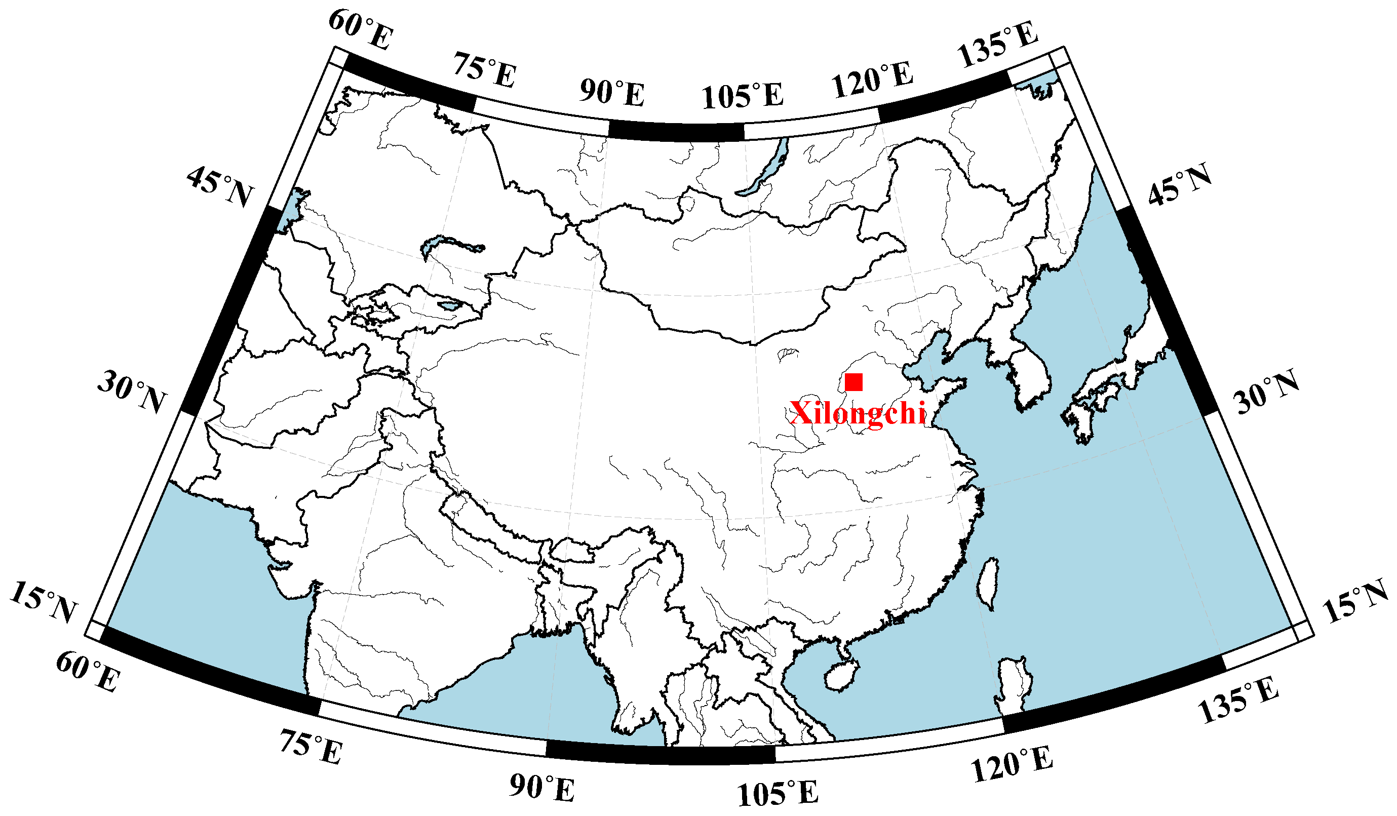
2.1.1. Introduction of Xilongchi Dam
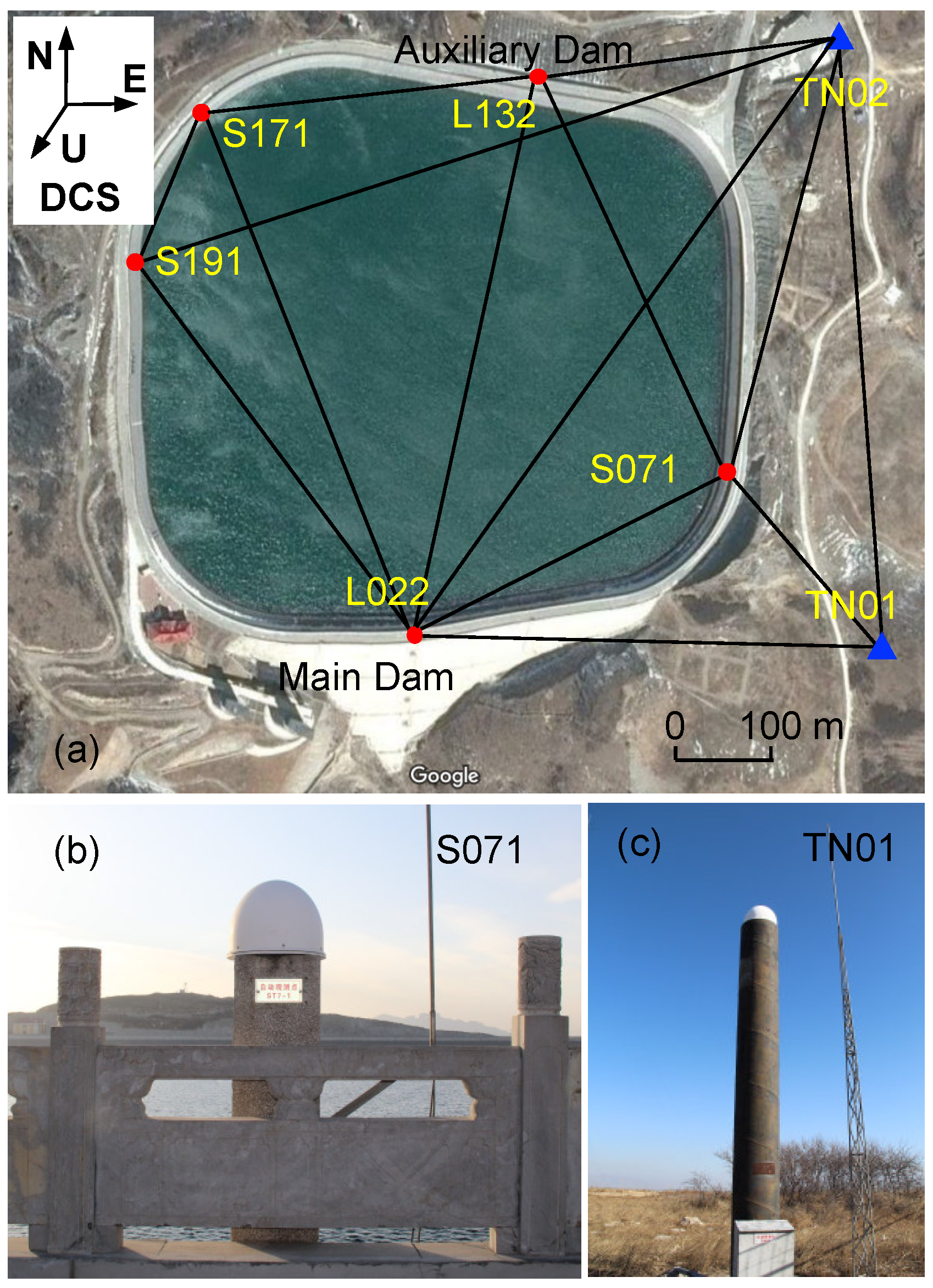
2.1.2. GPS Station Layout
2.1.3. Temperature and Water-Level Datasets
2.2. Methods
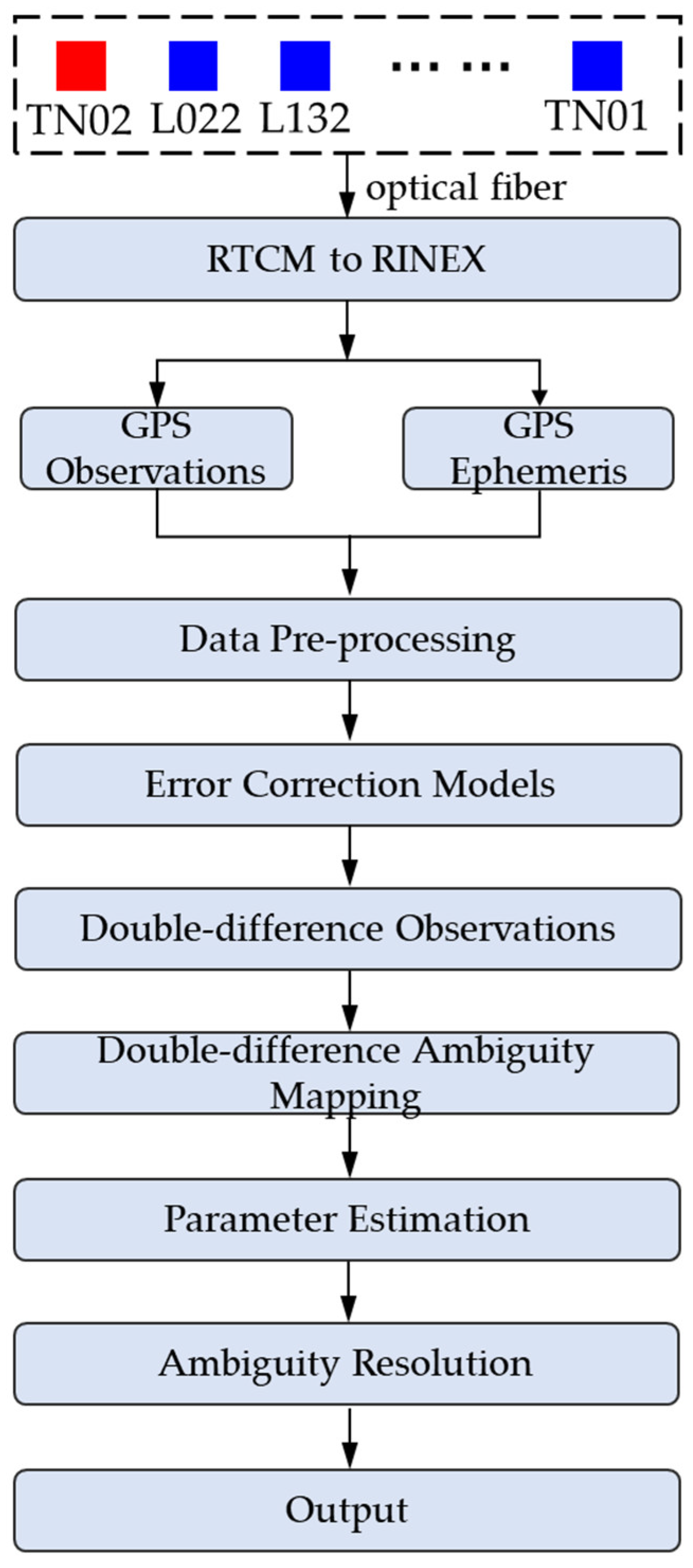
2.2.1. GPS Data Processing
2.2.2. Time-Series Analysis Method
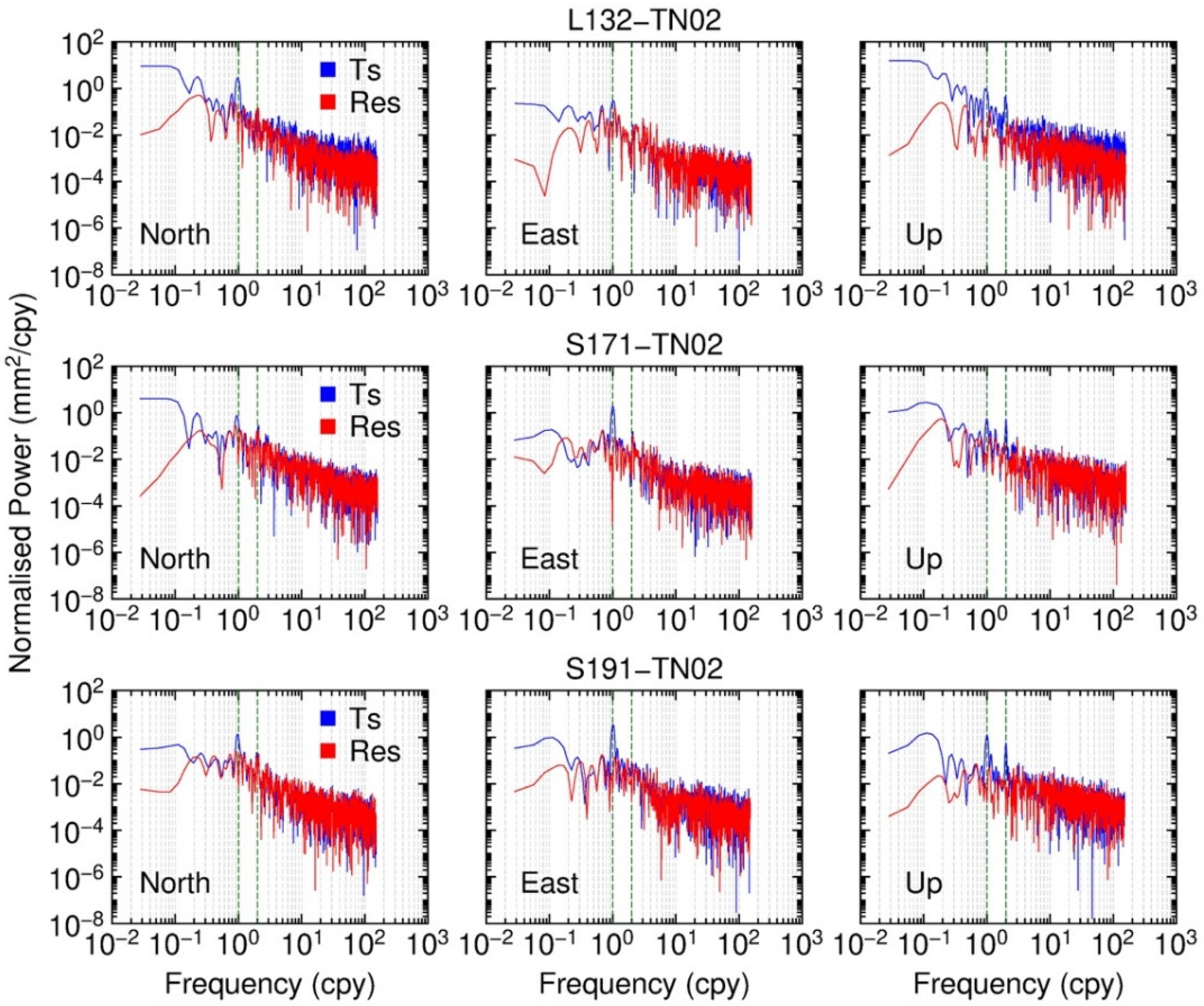
2.2.3. Lomb–Scargle Periodogram Method
3. Results
4. Discussion
4.1. Annual Signals
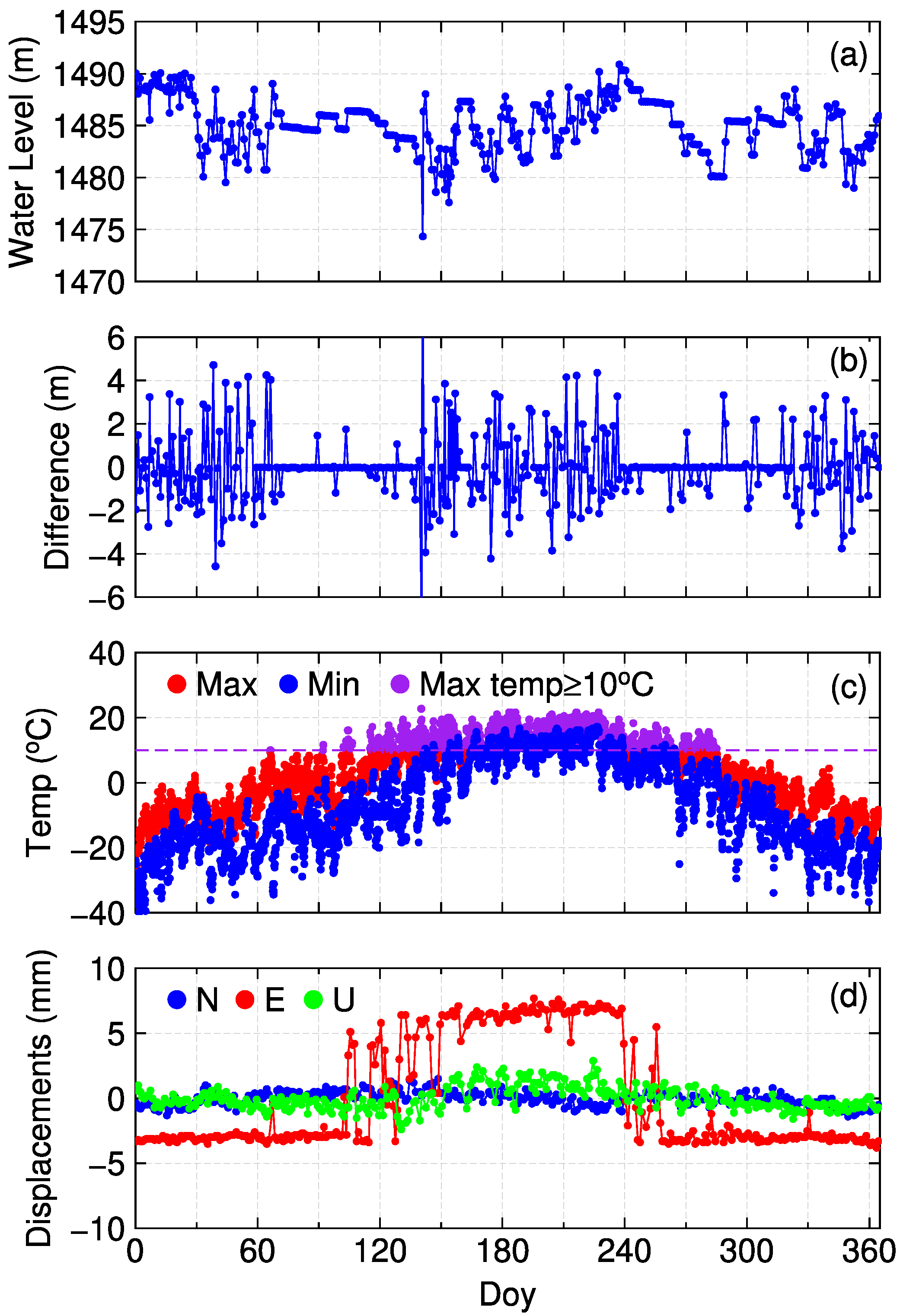
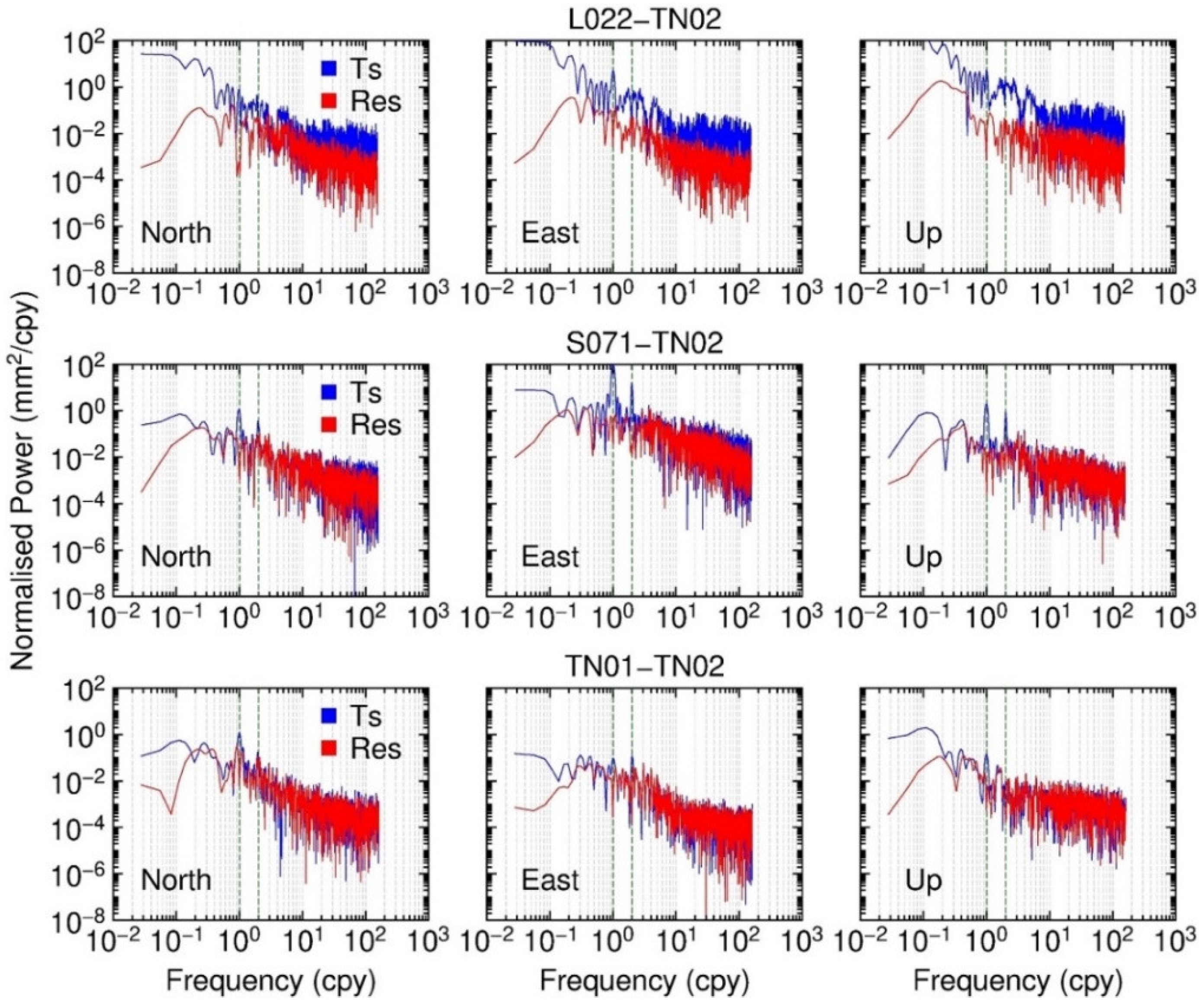
4.2. The Spurious Signals in the East Component of S071–TN02
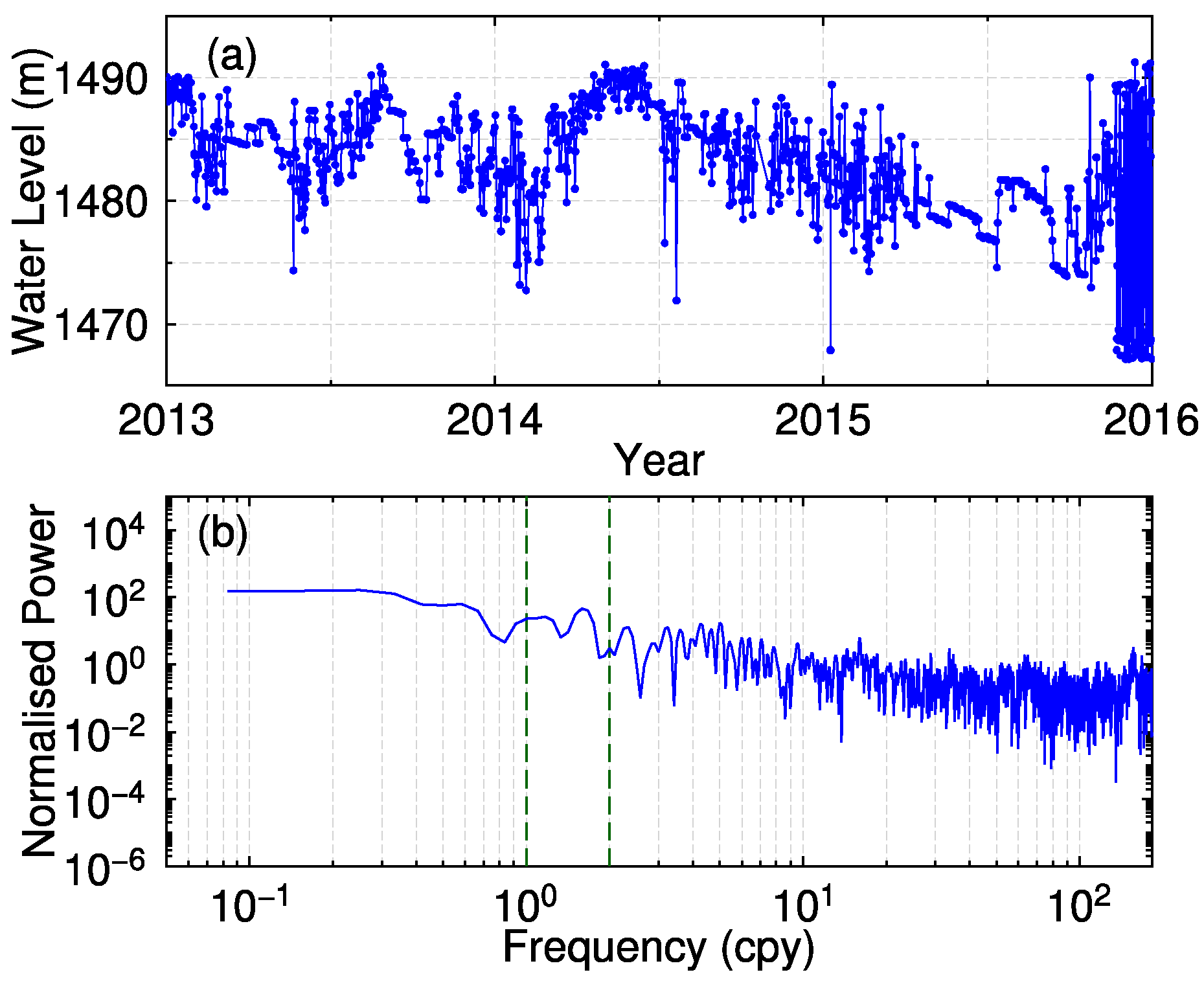
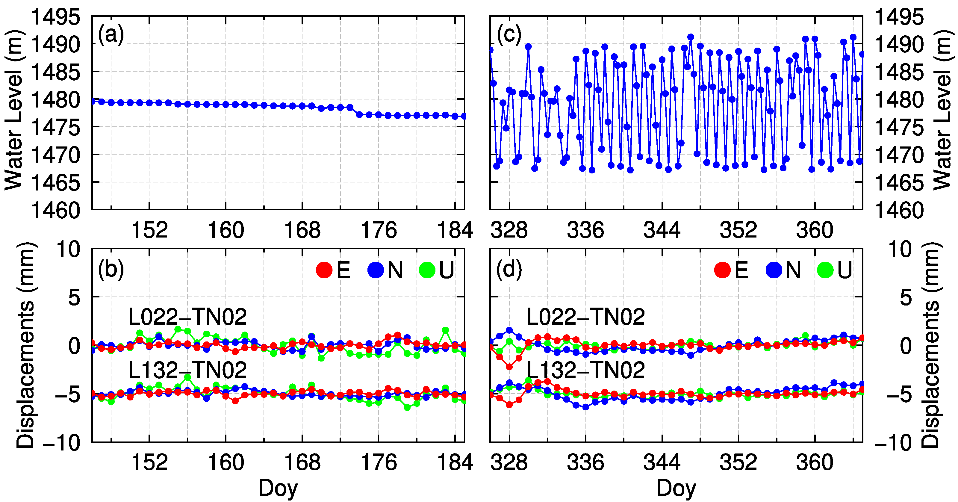
4.3. Water Level Variation
5. Conclusions
Author Contributions
Funding
Data Availability Statement
Conflicts of Interest
References
- Bukenya, P.; Moyo, P.; Beushausen, H.; Oosthuizen, C. Health monitoring of concrete dams: A literature review. Struct. Health Monit. 2014, 4, 235–244. [Google Scholar] [CrossRef]
- Ardito, R.; Maier, G.; Massalongo, G. Diagnostic analysis of concrete dams based on seasonal hydrostatic loading. Eng. Struct. 2008, 30, 3176–3185. [Google Scholar] [CrossRef]
- Behr, J.; Hudnut, K.; King, N. Monitoring structural deformation at Pacoima dam, California using continuous GPS. In Proceedings of the 11th International Technical Meeting of the Satellite Division of the Institute of Navigation, Nashville, TN, USA, 15–18 September 1998; pp. 59–68. [Google Scholar]
- Hudnut, K.W.; Behr, J.A. Continuous GPS Monitoring of Structural Deformation at Pacoima Dam, California. Seismol. Res. Lett. 1998, 69, 299–308. [Google Scholar] [CrossRef]
- Kulkarni, M.N.; Radhakrishnan, N.; Rai, D. Global positioning system in disaster monitoring of Koyna dam, Western Maharashtra. Surv. Rev. 2006, 38, 629–636. [Google Scholar] [CrossRef]
- Taşçi, L. Dam deformation measurements with GPS. Geod. Cartogr. 2008, 34, 116–121. [Google Scholar] [CrossRef]
- Gökalp, E.; Taşçı, L. Deformation monitoring by GPS at embankment dams and deformation analysis. Surv. Rev. 2009, 41, 86–102. [Google Scholar] [CrossRef]
- Ehiorobo, J.O.; Irughe-Ehigiator, R. Monitoring for horizontal movement in an earth dam using differential GPS. J. Emerg. Trends Eng. Appl. Sci. 2011, 2, 908–913. [Google Scholar]
- Kalkan, Y. Geodetic deformation monitoring of Ataturk Dam in Turkey. Arab. J. Geosci. 2014, 7, 397–405. [Google Scholar] [CrossRef]
- Acosta, L.; de Lacy, M.; Ramos, M.; Cano, J.; Herrera, A.; Avilés, M.; Gil, A. Displacements study of an earth fill dam based on high precision geodetic monitoring and numerical modeling. Sensors 2018, 18, 1369. [Google Scholar] [CrossRef]
- Barzaghi, R.; Cazzaniga, N.E.; De Gaetani, C.I.; Pinto, L.; Tornatore, V. Estimating and Comparing Dam Deformation Using Classical and GNSS Techniques. Sensors 2018, 18, 756. [Google Scholar] [CrossRef]
- Berkant, K.; Leyla, C.; Yilmaz, V. Monitoring the deformation of a concrete dam: A case study on the Deriner Dam, Artvin, Turkey. Geomat. Nat. Haz. Risk 2020, 11, 160–177. [Google Scholar]
- Xi, R.; Zhou, X.; Jiang, W.; Chen, Q. Simultaneous estimation of dam displacements and reservoir level variation from GPS measurements. Measurement 2018, 122, 247–256. [Google Scholar] [CrossRef]
- Xiao, R.; Shi, H.; He, X.; Li, Z.; Jia, D.; Yang, Z. Deformation Monitoring of Reservoir Dams Using GNSS: An Application to South-to-North Water Diversion Project, China. IEEE Access 2019, 7, 54981–54992. [Google Scholar] [CrossRef]
- Pytharouli, S.I.; Stiros, S.C. Ladon dam (Greece) deformation and reservoir level fluctuations: Evidence for a causative relationship from the spectral analysis of a geodetic monitoring record. Eng. Struct. 2005, 27, 361–370. [Google Scholar] [CrossRef]
- Bayrak, T. Modelling the relationship between water level and vertical displacements on the Yamula Dam. Nat. Hazards Earth Syst. Sci. 2007, 7, 289–297. [Google Scholar] [CrossRef]
- Léger, P.; Leclerc, M. Hydrostatic, temperature, time-displacement model for concrete dams. J. Eng. Mech. 2007, 133, 267–277. [Google Scholar] [CrossRef]
- De Sortis, A.; Paoliani, P. Statistical analysis and structural identification in concrete dam monitoring. Eng. Struct. 2007, 29, 110–120. [Google Scholar] [CrossRef]
- Lew, J.S.; Loh, C.H. Structural health monitoring of an arch dam from static deformation. J. Civ. Struct. Health Monit. 2014, 4, 245–253. [Google Scholar] [CrossRef]
- Loh, C.H.; Chen, C.H.; Hsu, T.Y. Application of advanced statistical methods for extracting long-term trends in static monitoring data from an arch dam. Struct. Health Monit. Int. J. 2011, 10, 587–601. [Google Scholar] [CrossRef]
- Hsu, T.Y.; Loh, C.H. Damage detection accommodating nonlinear environmental effects by nonlinear principal component analysis. Struct. Control Health Monit. 2010, 17, 338–354. [Google Scholar] [CrossRef]
- Huang, Y.; Schmitt, F.G.; Lu, Z.; Liu, Y. Analysis of daily river flow fluctuations using empirical mode decomposition and arbitrary order Hilbert spectral analysis. J. Hydrol. 2009, 373, 103–111. [Google Scholar] [CrossRef]
- Agnieszka, W.; Dawid, K. Modeling seasonal oscillations in GNSS time series with Complementary Ensemble Empirical Mode Decomposition. GPS Solut. 2022, 26, 10. [Google Scholar] [CrossRef]
- King, M.A.; Williams, S.D.P. Apparent stability of GPS monumentation from short-baseline time series. J. Geophys. Res. 2009, 114, 1–21. [Google Scholar] [CrossRef]
- Hill, E.M.; Davis, J.L.; Elósegui, P.; Wernicke, B.P.; Malikowski, E.; Niemi, N.A. Characterization of site-specific GPS errors using a short-baseline network of braced monuments at Yucca Mountain, southern Nevada. J. Geophys. Res.-Solid Earth 2009, 114, 1–13. [Google Scholar] [CrossRef]
- Liu, H.; Xiao, Y.; Deng, L.; Bi, G. Analysis of long-term stability of reference stations in GPS deformation monitoring system. J. Geod. Geodyn. 2013, 33, 113–122. (In Chinese) [Google Scholar]
- Liu, X. Xilongchi Upper Reservoir GPS Data Processing and its Time Series Analysis. Master’s Thesis, Wuhan University, Wuhan, China, 2015. (In Chinese). [Google Scholar]
- Herring, T.A.; King, R.W.; Floyd, M.A.; McClusky, S.C. GAMIT-GPS Analysis at MIT, Reference Manual 10.6; Department of Earth, Atmospheric, and Planetary Sciences Massachusetts Institute of Technology: Cambridge, MA, USA, 2015. [Google Scholar]
- Dong, D.; Bock, Y. Global Positioning System network analysis with phase ambiguity resolution applied to crustal deformation studies in California. J. Geophys. Res. Solid Earth 1989, 94, 3949–3966. [Google Scholar] [CrossRef]
- King, M.A.; Watson, C.S. Long GPS coordinate time series: Multipath and geometry effects. J. Geophys. Res. 2010, 115, 1–23. [Google Scholar] [CrossRef]
- King, M.A.; Watson, C.S.; Penna, N.T.; Clarke, P.J. Subdaily signals in GPS observations and their effect at semiannual and annual periods. Geophys. Res. Lett. 2008, 35, 1–5. [Google Scholar] [CrossRef]
- Bos, M.; Fernandes, R.; Williams, S.; Bastos, L. Fast error analysis of continuous GNSS observations with missing data. J. Geod. 2013, 87, 351–360. [Google Scholar] [CrossRef]
- Liu, H.; Li, L. Missing Data Imputation in GNSS Monitoring Time Series Using Temporal and Spatial Hankel Matrix Factorization. Remote Sens. 2022, 14, 1500. [Google Scholar] [CrossRef]
- Pytharouli, S.I.; Stiros, S.C. Spectral analysis of unevenly spaced or discontinuous data using the “normperiod” code. Comput. Struct. 2008, 86, 190–196. [Google Scholar] [CrossRef]
- Ghaderpour, E. Least-squares Wavelet and Cross-wavelet Analyses of VLBI Baseline Length and Temperature Time Series: Fortaleza–Hartebeesthoek–Westford–Wettzell. Publ. Astron. Soc. Pac. 2021, 133, 014502. [Google Scholar] [CrossRef]
- Ghaderpour, E.; Pagiatakis, S.D. LSWAVE: A MATLAB software for the least-squares wavelet and cross-wavelet analyses. GPS Solut. 2019, 23, 50. [Google Scholar] [CrossRef]
- Ghaderpour, E.; Ince, E.S.; Pagiatakis, S.D. Least-squares cross-wavelet analysis and its applications in geophysical time series. J. Geod. 2018, 92, 1223–1236. [Google Scholar] [CrossRef]
- Ghaderpour, E. JUST: MATLAB and python software for change detection and time series analysis. GPS Solut. 2021, 25, 85. [Google Scholar] [CrossRef]
- Lomb, N.R. Least-squares frequency analysis of unequally spaced data. Astrophys. Space Sci. 1976, 39, 447–462. [Google Scholar] [CrossRef]
- Scargle, J.D. Studies in astronomical time series analysis. II. Statistical aspects of spectral analysis of unevenly spaced data. Astron. J. 1982, 263, 835–853. [Google Scholar] [CrossRef]
- Jiang, W.; Li, Z.; van Dam, T.; Ding, W. Comparative analysis of different environmental loading methods and their impacts on the GPS height time series. J. Geod. 2013, 87, 687–703. [Google Scholar] [CrossRef]
- Jiang, W.; Liu, H.; Zhou, X.; Li, Z. Analysis of long-term deformation of reservoir using continuous GPS observations. Acta Geod. Cartogr. Sin. 2012, 41, 682–689. (In Chinese) [Google Scholar]
- Dong, D.; Fang, P.; Bock, Y.; Cheng, M.K.; Miyazaki, S. Anatomy of apparent seasonal variations from GPS-derived site position time series: Seasonal variations from GPS site time series. J. Geophys. Res.-Solid Earth 2002, 107, ETG 9-1–ETG 9-16. [Google Scholar] [CrossRef]
- Yan, H.; Chen, W.; Zhu, Y.; Zhang, W.; Zhong, M.; Liu, G. Thermal effects on vertical displacement of GPS stations in China. Chin. J. Geophys. 2010, 53, 825–832. (In Chinese) [Google Scholar] [CrossRef]


| Baseline | N (m) | E (m) | U (m) | Length (m) | Data Integrity (%) |
|---|---|---|---|---|---|
| L022–TN02 | 487.95 | 407.59 | 13.91 | 635.94 | 96.40 |
| L132–TN02 | 33.35 | 289.17 | 13.83 | 291.42 | 97.73 |
| S171–TN02 | 56.75 | 565.22 | 13.37 | 568.22 | 92.63 |
| S191–TN02 | 188.17 | 621.74 | 13.40 | 649.73 | 93.95 |
| S071–TN02 | 354.00 | 122.69 | 13.33 | 374.90 | 96.06 |
| TN01–TN02 | 511.67 | −11.00 | −1.70 | 511.79 | 97.34 |
| Model and Parameters | Static Solution |
|---|---|
| Software | GAMIT 10.6 |
| Observation | L1_only |
| Baseline processing | Network solution |
| Estimator | Least squares |
| Elevation cutoff | 15° |
| Tropospheric zenith delay (TZD) | Differenced |
| Ionospheric delay | Differenced |
| Sampling rate | 30 s |
| Observation weighting model | Elevation weight model |
| Orbit | IGS final orbit (fixed) |
| Ambiguity resolution | Bootstrapping + decision function method [29] |
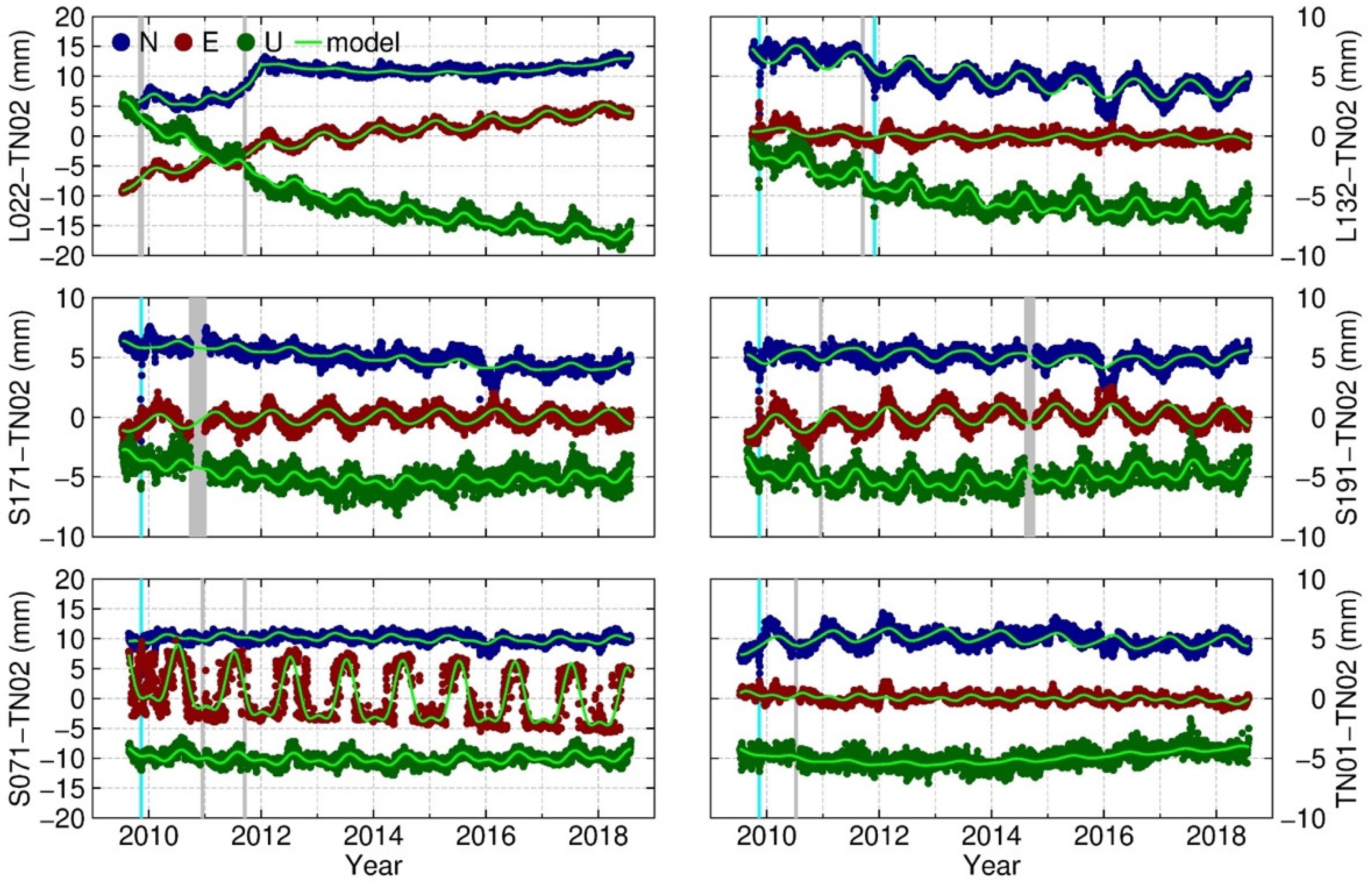
| Baseline | Component | Linear Trend | Annual Amplitude | Semiannual Amplitude |
|---|---|---|---|---|
| L022–TN02 | N 1 | −0.2 | 0.7 | 0.3 |
| N 2 | 0.0 | 0.2 | 0.1 | |
| E | 1.0 | 1.0 | 0.1 | |
| U | −1.8 | 0.9 | 0.4 | |
| L132–TN02 | N | −0.5 | 0.9 | 0.1 |
| E | 0.0 | 0.3 | 0.0 | |
| U | −0.4 | 0.6 | 0.4 | |
| S171–TN02 | N | −0.3 | 0.3 | 0.1 |
| E | 0.0 | 0.6 | 0.1 | |
| U | 0.0 | 0.3 | 0.3 | |
| S191–TN02 | N | −0.2 | 0.5 | 0.1 |
| E | 0.0 | 0.9 | 0.1 | |
| U | 0.2 | 0.6 | 0.4 | |
| S071–TN02 | N | −0.2 | 0.5 | 0.3 |
| E | −0.2 | 4.8 | 2.0 | |
| U | 0.0 | 0.7 | 0.5 | |
| TN01–TN02 | N | −0.2 | 0.5 | 0.1 |
| E | 0.0 | 0.1 | 0.2 | |
| U | 0.2 | 0.2 | 0.1 |
| Prefit RMS (mm) | Postfit RMS (mm) | |||||
|---|---|---|---|---|---|---|
| Baseline | N | E | U | N | E | U |
| L022–TN02 | 2.3 | 3.4 | 6.1 | 0.5 | 0.5 | 0.9 |
| L132–TN02 | 1.4 | 0.5 | 1.6 | 0.5 | 0.4 | 0.5 |
| S171–TN02 | 0.9 | 0.7 | 1.0 | 0.6 | 0.5 | 0.7 |
| S191–TN02 | 0.7 | 0.9 | 0.9 | 0.6 | 0.5 | 0.6 |
| S071–TN02 | 0.8 | 4.4 | 0.9 | 0.6 | 2.2 | 0.7 |
| TN01–TN02 | 0.7 | 0.4 | 0.7 | 0.5 | 0.3 | 0.5 |
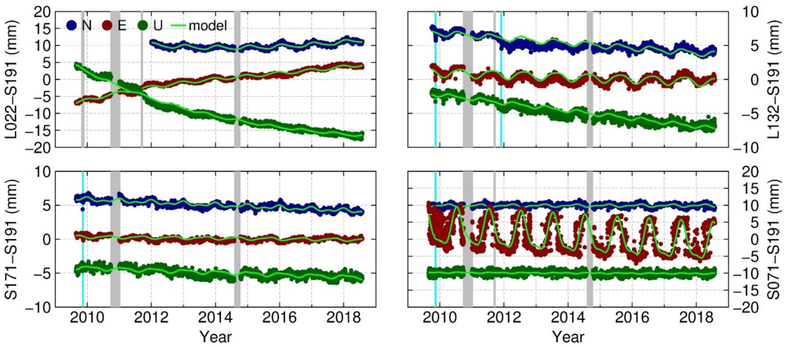
| Baseline | Component | Linear Trend | Annual Amplitude | Reduced Percentage of Annual Amplitude | Semiannual Amplitude | Reduced Percentage of Semiannual Amplitude |
|---|---|---|---|---|---|---|
| L022–S191 | N 2 | 0.2 | 0.6 | −150.8% | 0.1 | −48.1% |
| E | 1.0 | 0.5 | 53.9% | 0.0 | 58.3% | |
| U | −2.0 | 0.3 | 62.6% | 0.1 | 80.1% | |
| L132- S191 | N | −0.4 | 0.4 | 54.6% | 0.1 | −38.3% |
| E | −0.2 | 0.6 | −130.4% | 0.1 | −104.2% | |
| U | −0.6 | 0.2 | 60.4% | 0.1 | 72.2% | |
| S171- S191 | N | −0.2 | 0.2 | 29.2% | 0.2 | −38.7% |
| E | −0.0 | 0.2 | 68.0% | 0.1 | 11.1% | |
| U | −0.2 | 0.3 | 38.5% | 0.1 | 69.0% | |
| S071- S191 | N | 0.0 | 0.3 | 35.0% | 0.2 | 24.6% |
| E | −0.5 | 5.2 | −7.4% | 1.7 | 12.2% | |
| U | −0.0 | 0.1 | 84.2% | 0.1 | 75.4% |
| Baselines | Before Removing Fitting Models | After Removing Fitting Models | ||||
|---|---|---|---|---|---|---|
| N | E | U | N | E | U | |
| L022–S191 | 0.8 | 3.0 | 5.7 | 0.3 | 0.4 | 0.7 |
| L132–S191 | 0.9 | 0.6 | 1.5 | 0.5 | 0.5 | 0.5 |
| S171–S191 | 0.6 | 0.3 | 0.6 | 0.3 | 0.3 | 0.4 |
| S071–S191 | 0.5 | 4.6 | 0.6 | 0.4 | 2.6 | 0.6 |
| Year | ETS > 5.0 mm | 5.0 mm > ETS > −3.0 mm | ETS < −3.0 mm | ||||||
|---|---|---|---|---|---|---|---|---|---|
| T > 10 °C | 10 °C > T > 0 °C | T < 0 °C | T > 10 °C | 10 °C > T > 0 °C | T < 0 °C | T > 10 °C | 10 °C > T > 0 °C | T < 0 °C | |
| 2010 | 67.89 | 19.27 | 12.84 | 7.25 | 32.61 | 60.14 | 2.63 | 39.47 | 57.89 |
| 2011 | 86.08 | 12.66 | 1.27 | 6.38 | 47.87 | 45.74 | 0.00 | 12.71 | 87.29 |
| 2012 | 86.42 | 12.35 | 1.23 | 8.67 | 38.73 | 52.60 | 0.00 | 16.44 | 83.56 |
| 2013 | 96.39 | 3.61 | 0.00 | 15.85 | 41.46 | 42.68 | 1.86 | 21.74 | 76.40 |
| 2014 | 89.13 | 10.87 | 0.00 | 8.06 | 48.39 | 43.55 | 0.00 | 38.64 | 61.36 |
| 2015 | 80.23 | 18.60 | 1.16 | 14.29 | 52.86 | 32.86 | 0.00 | 21.48 | 78.52 |
Publisher’s Note: MDPI stays neutral with regard to jurisdictional claims in published maps and institutional affiliations. |
© 2022 by the authors. Licensee MDPI, Basel, Switzerland. This article is an open access article distributed under the terms and conditions of the Creative Commons Attribution (CC BY) license (https://creativecommons.org/licenses/by/4.0/).
Share and Cite
Xi, R.; Liang, Y.; Chen, Q.; Jiang, W.; Chen, Y.; Liu, S. Analysis of Annual Deformation Characteristics of Xilongchi Dam Using Historical GPS Observations. Remote Sens. 2022, 14, 4018. https://doi.org/10.3390/rs14164018
Xi R, Liang Y, Chen Q, Jiang W, Chen Y, Liu S. Analysis of Annual Deformation Characteristics of Xilongchi Dam Using Historical GPS Observations. Remote Sensing. 2022; 14(16):4018. https://doi.org/10.3390/rs14164018
Chicago/Turabian StyleXi, Ruijie, Yuhan Liang, Qusen Chen, Weiping Jiang, Yan Chen, and Simin Liu. 2022. "Analysis of Annual Deformation Characteristics of Xilongchi Dam Using Historical GPS Observations" Remote Sensing 14, no. 16: 4018. https://doi.org/10.3390/rs14164018
APA StyleXi, R., Liang, Y., Chen, Q., Jiang, W., Chen, Y., & Liu, S. (2022). Analysis of Annual Deformation Characteristics of Xilongchi Dam Using Historical GPS Observations. Remote Sensing, 14(16), 4018. https://doi.org/10.3390/rs14164018