Abstract
Deep-learning (DL)-based object detection algorithms can greatly benefit the community at large in fighting fires, advancing climate intelligence, and reducing health complications caused by hazardous smoke particles. Existing DL-based techniques, which are mostly based on convolutional networks, have proven to be effective in wildfire detection. However, there is still room for improvement. First, existing methods tend to have some commercial aspects, with limited publicly available data and models. In addition, studies aiming at the detection of wildfires at the incipient stage are rare. Smoke columns at this stage tend to be small, shallow, and often far from view, with low visibility. This makes finding and labeling enough data to train an efficient deep learning model very challenging. Finally, the inherent locality of convolution operators limits their ability to model long-range correlations between objects in an image. Recently, encoder–decoder transformers have emerged as interesting solutions beyond natural language processing to help capture global dependencies via self- and inter-attention mechanisms. We propose Nemo: a set of evolving, free, and open-source datasets, processed in standard COCO format, and wildfire smoke and fine-grained smoke density detectors, for use by the research community. We adapt Facebook’s DEtection TRansformer (DETR) to wildfire detection, which results in a much simpler technique, where the detection does not rely on convolution filters and anchors. Nemo is the first open-source benchmark for wildfire smoke density detection and Transformer-based wildfire smoke detection tailored to the early incipient stage. Two popular object detection algorithms (Faster R-CNN and RetinaNet) are used as alternatives and baselines for extensive evaluation. Our results confirm the superior performance of the transformer-based method in wildfire smoke detection across different object sizes. Moreover, we tested our model with 95 video sequences of wildfire starts from the public HPWREN database. Our model detected 97.9% of the fires in the incipient stage and 80% within 5 min from the start. On average, our model detected wildfire smoke within 3.6 min from the start, outperforming the baselines.
1. Introduction
1.1. Motivation
There were more than 58,000 wildfires recorded in the United States in 2021, which have burned more than seven million acres [1,2]. The condition is particularly worse for the Western United States, where ninety percent of the land is impacted by severe drought. In California, fire seasons have been starting earlier and lasting longer. The five-year average cost of fire fighting in the U.S. is USD 2.35 billion [3]. Furthermore, researchers [4] have found evidence to associate fine particles found in wildfire smoke to repository morbidity and complications in general. The shear damage and suppression costs of wildfires have motivated many researchers to develop systems to detect fire at the early stages.

Figure 1.
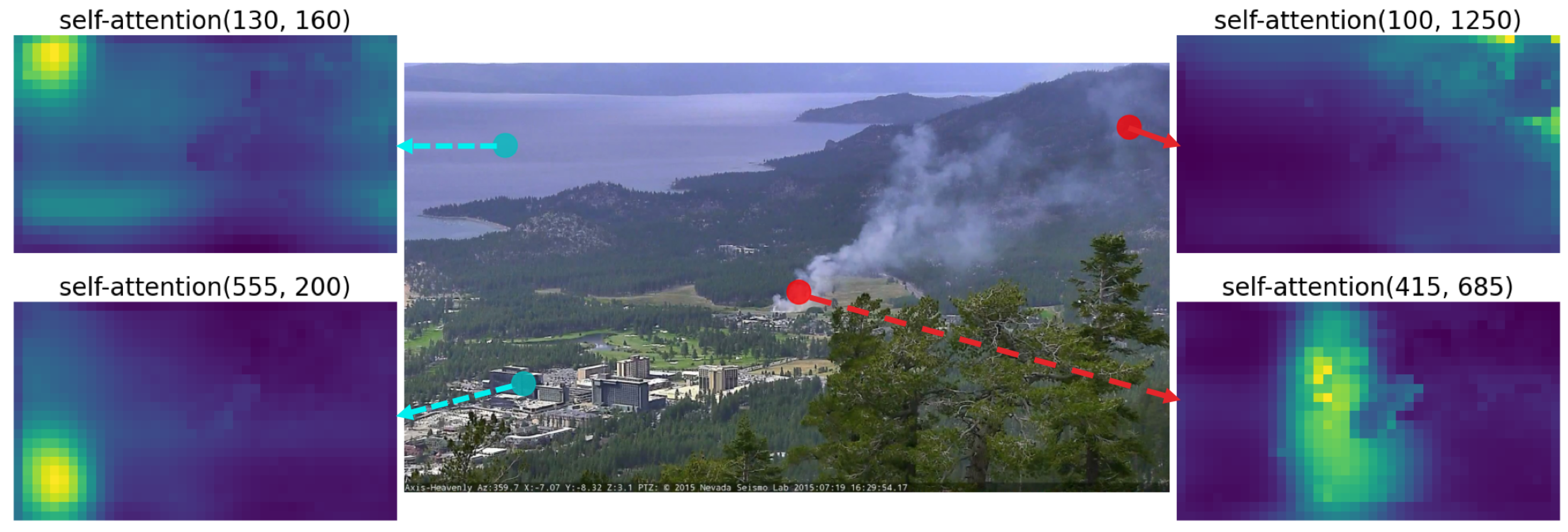
Encoder self-attention for a set of reference points. The example shows that the encoder is able to separate instances and regions, even at the early stages of training.
Figure 1.
Encoder self-attention for a set of reference points. The example shows that the encoder is able to separate instances and regions, even at the early stages of training.
The first detection systems were based on typical fire-sensing technologies such as gas, heat, and smoke detectors. Conventional sensors have a limited range and coverage, while suffering from a slow response time, as smoke particles need to reach the sensors to activate them [5,6]. Later works were based on optical remote sensing at three different acquisition levels: satellite, aerial, and terrestrial. References [7,8,9] leveraged satellite remote sensing to detect fire. Satellites offer extensive views of the Earth’s surface; however, they suffer from a relatively coarse spatial and temporal resolution and, thus, are only effective in the detection and monitoring of large-scale forest fires [10]. Moreover, satellites operating in Low Earth Orbit (LEO) offer finer resolutions, making them more suitable for detecting fire in the early phases, but take a long time to re-position and thus have limited coverage [11]. Ideally, a constellation of low-orbit satellites with reliable and fast network capabilities can provide the required coverage [11]. Aerial remote sensing approaches, such as deploying sensors on high-altitude aircraft and balloons, have also been tried, but they are costly or have limited coverage [11].
Finally, a terrestrial option to sense fire would be optical cameras installed at good vantage points. Two large-scale networks of such cameras are already deployed in the Western United States. AlertWildfire [12] provides access to 900 cameras across eight states, while HPWREN [13] provides a comprehensive coverage of the wildfire-prone Southern California. The placement of these cameras enables a range view of up to 50 miles [14]. Some are also capable of panning, tilting, and zooming (PTZ), offering additional options to monitor wildfires at different resolutions. In this paper, we use the videos from these two networks as our raw input data for training and evaluating our deep-learning-based wildfire smoke detectors, an example of which is shown in Figure 1. The frames extracted from these raw videos are mostly 2 Mega Pixels (MP), with 3 MP and 6 MP the next-most-common dimensions in the dataset.
Wildfires typically ignite in rural and remote areas, such as forests, using abundant wildland vegetation as fuel [15]. They spread quickly and uncontrollably, making them difficult to control in a short time. Thus, the most important objective of any wildfire detection system is to detect wildfires early and before they grow [15]. This is called the incipient stage of fire development. Wildfires in the incipient stage comprise a non-flaming smoldering with relatively low heat. Recognizing fire at this stage offers the best chance of suppression. Moreover, flame is not typically visible at this stage; thus, any wildfire detection system that aims at early detection must focus on detecting smoke and not flame. Additionally, the smoke plume at this stage tends to be very small and, in some cases, not visible [11,16] by human observation of wildfire videos, especially in the first few minutes after the start of the fire. Thus, any wildfire detection system tailored to early detection should be able to detect small smoke plumes, typically far from view and on the horizon.
1.2. Challenges
After an extensive review of the literature, we found that the majority of works have a holistic approach towards fire stages and do not focus on a particular stage (e.g., incipient). The fastest wildfire smoke detection method that we know of [16] reported a 6.3 min detection latency based on 24 challenging wildfire sequences (i.e., a 9 min detection latency after converting their reference times to the official start times reported in the HPWREN database [17]). Moreover, the majority of existing works [10,18,19,20,21,22,23,24,25,26,27,28,29,30,31] do not distinguish between flame and smoke or simply focus on flame, which has more pronounced features, is easier to detect, and is mostly visible only in the more advanced stages. Furthermore, a significant number of works detect smoke or flame at relatively close range [18,19,20,21,22,23,32,33,34,35], such as using CCTV cameras in indoor or urban environments [24,25,26,27]. We only know of one study [16] that explicitly focuses on detecting smoke plumes on the horizon.
We believe the main reason why the literature is lacking in long-range and early incipient smoke detection is the shear difficulty of finding, processing, and annotating smoke bounding boxes at this stage. Smoke at this stage tends to be extremely small, shallow, and in some cases, only visible through careful and repetitive observation of video footage and zooming. Interestingly, there is no lack of databases of raw videos and images of wildlands and wildfire scenes, thanks to the prevalence of terrestrial remote sensing networks such as [12,13]. However, there is a lack of processed, open-source, and labeled data for early bounding box detection of wildfire smoke. Most existing works have some commercial or proprietary aspect [16,36,37] or share only a subset of their labeled data [11].
We noticed a common trend in the existing deep-learning-based studies. They are all based on convolutional neural networks (ConvNets or CNNs). Some of the works attempt to indirectly localize smoke regions through a moving window approach combined with secondary image classification [11,21,38], while others are based on more sophisticated object detection methods such as Faster R-CNN with feature pyramid networks (FPNs) [39], EfficientDet [40], RetinaNet [41], and Yolo [42,43], to predict and localize flame and smoke bounding boxes. However, what all ConvNets have in common is the inherent locality of convolutional filters, which limits the model in exploring all the possible long-range relationships between elements of an image. Moreover, such systems are typically anchor-based, and their performance and generalizability are limited to the design of the anchors. In addition, the inference speed and accuracy is heavily impacted by image size [11].
1.3. Nemo: An Open-Source Transformer-Supercharged Benchmark for Fine-Grained Wildfire Smoke Detection
We hypothesize that, to improve upon the CNN-based wildfire detection methods, especially in terms of detection rate in the early incipient stage, size of smoke, and detection range, we need a method that can tap into the long-range dependencies between image pixels. We found encoder–decoder Transformers to be a promising solution, as the global computation and perfect memory of attention-based mechanisms have already made them the superior model for long sequences, particularly in problems such as natural language processing (NLP) and speech recognition [44]. Very recently, visual Transformers have shown outstanding results in the prediction of natural hazards, such as landslides [45] and wildfire flame [46]. We hypothesize that the global attention of the encoder layer can help capture long-range dependencies in the large images of our dataset, in a similar fashion to how attention mechanisms capture latent relationships in long sentences in NLP. We also found a general-purpose object detection tool based on Transformers, namely DEtection TRansformer (DETR) [47].
To fill the gaps, we propose a novel benchmark, namely the Nevada Smoke detection benchmark (Nemo), for wildfire smoke and fine-grained smoke density detection. Nemo is an evolving collection of labeled and processed datasets and trained DL-based wildfire smoke (and smoke density) detectors, freely available to the research community [48]. To the best of our knowledge, this is the first open-source benchmark for wildfire smoke density detection and wildfire smoke detection tailored to the early incipient stage. To create our dataset, we collect, process, and label thousands of images from raw videos for the purpose of bounding box detection of wildfire smoke. We mainly focus our preprocessing efforts on the earliest minutes of smoke visibility (i.e., early incipient stage). Furthermore, we create a finer-grained version of our labeled annotations to further divide the smoke region into three subcategories based on perceived smoke density. The overarching goal of the fine-grained smoke detection is to help differentiate particles of smoke based on their thickness, opacity, and density, which typically associates with the severity of smoke (i.e., thicker smoke being more severe). This can have potential applications in climate intelligence such as predicting pollutants and hazards.
Our main wildfire smoke detectors are based on encoder–decoder Transformers, and in particular on Facebook’s Detection Transformer (DETR) [47]. DETR is an end-to-end, one-stage object detector, meaning it has removed the need for anchor generation and second-stage refinements. DETR is trained on the COCO dataset of 80 everyday objects, such as person, car, TV, etc. We transfer weights from the DETR COCO object detector, but remove the classification head (i.e., class weights and biases), and then load the state dictionary from the transferred model. To adapt it to smoke detection, we also change the input dimension of the decoder by removing the query embeddings and replace it with a different set of queries, learned for the smoke detection use-case. All the other intermediary weights and biases were kept from the transferred model to help reduce the training schedule. To the best of our knowledge, this is the first study on the Transformer architecture for early wildfire detection. There exists another work [46] that uses visual Transformers, but for wildfire flame segmentation, which is both a separate task (i.e., panoptic segmentation) and different target object (i.e., flame). The main contributions of this study are summarized as follows:
- We show that the self- and inter-attention mechanisms of encoder–decoder Transformers utilize long-range relationships and global reasoning to achieve state-of-the-art performance for wildfire smoke and smoke density detection. An example visualization of the encoder self-attention weights from a model we trained on our data is shown in Figure 1. This shows that even at an early stage of training (i.e., encoding), the model already attends to some form of instance separation.
- Additionally, our benchmark offers trained smoke detectors based on well-established and highly optimized object detection algorithms, namely Faster R-CNN with FPN [39] and RetinaNet [41]. The reasons for choosing these alternative object detection algorithms were their impressive results in incipient stage smoke detection, reported in a recent work [16], and to provide a comparison and context for our Transformer-based smoke detector. Our results based on numerous visual inferences and popular object detection metrics (i.e., mAP, PASCAL VOC, etc.) show that the encoder–decoder Transformer architecture performs better than the state-of-the-art ConvNets for wildfire detection.
- We also create additional dataset configurations, motivated by our initial results, which returned a relatively high number of false detections in a challenging set of empty images. We add collage images of smoke and non-smoke scenes. Our results show a significant reduction of false alarms for all models. We also created an alternative dataset, tailored to situations where the underlying object detection codebase does not support explicit addition of negative samples for training.
- Furthermore, we perform an extensive time-series analysis on a large test set, collected exclusively from the incipient stage of 95 wildfires [13,17]. From time-stamps recorded on the 95 video sequences and our detection results, we determined the mean time of detection after the start of the fire (i.e., mean detection delay, or latency). To the best of our knowledge, this is the largest analysis of its kind. Our Transformer-supercharged detector can predict wildfire smoke within 3.6 min from the start of the fire, on average. In context, we compared our results to 16 video sequences used in a similar analysis from [16]. We show that our model detects wildfire smoke more than 7 min faster than the best-performing model reported in the literature [16]. Our model was able to detect 97.9% of the wildfires within the incipient stage and more than two-thirds of the fires within 3 min. Since the majority of the smoke columns in the first few minutes of a fire are extremely small, far, and shallow, then by extension, we confirm that the proposed models are effective at detecting small fires. For instance, our model was able to detect objects as small as 24 by 26 pixels in an image of 3072 by 2048 pixels (6 MP). In relative terms, the correctly detected smoke object is 0.0099% of the input image, as shown in Figure 2.
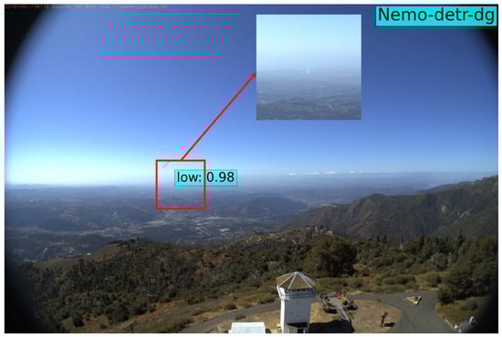 Figure 2. A tiny column of smoke near the horizon is correctly detected as low-density smoke, two minutes after the start of the fire. Viewed from a west-facing fixed camera on top of Palomar Mountain, California, on 1 October 2019. The smoke object is 24 × 26 pixels wide, and the image is 3072 × 2048 pixels, which makes the detected object less than 0.01% of the image. A focused 300 by 300 cutout of the smoke area is shown, with the smoke column centered.
 - In addition, our Transformer-based detectors obtain more than 50% and 80% average precision (AP) for small and large objects, respectively, outperforming the baselines by more than 20% and 6%, respectively. This shows that our models are also effective at detecting larger fires in an advanced stage, which is an easier task, albeit still important, since it demonstrates the accuracy and applicability of our model in the continuous monitoring of developing wildfires.
The overarching objective of this study is to provide a free, open-source repository with labeled wildfire data and state-of-the-art smoke detectors with the core principal of repeatability and ease of use for the research community. We made our annotations, images, and trained models freely available at [48].
2. Background
2.1. State-of-the-Art
In this section, we discuss related work including state-of-the-art wildfire detection methods as summarized in Table 1. To the best of our knowledge, in terms of the approach, all existing works fall within the following main categories: (1) image processing and feature-based machine learning; (2) data-driven/deep-learning-based methods that also include the newer Transformer architecture.

Table 1.
State of fire detection. Main differences between existing studies are summarized, using 3 categories for brevity.
2.1.1. Image Processing and Feature-Based Wildfire Detection Methods
The earliest fire detection systems were based on infrared and ultraviolet sensors and were heavily impacted by false alarms [53]. They merely produced a signal determining fire without any indication of the location and size. Later works mostly used color features to identify fire from the background, using different color schemes and channels, such as red, green, blue (RGB) [54] and hue, saturation, intensity (HSI) [55]. However, these methods fail to detect fire reliably as they are sensitive to changes in illumination and choosing the exact fire pixel range (i.e., 0–255) can be very difficult. The results showed that color features alone are not sufficient to reliably detect fire.
Later detection methods incorporated a combination of static (e.g., colors, shapes, texture unique to fire) and dynamic (e.g., motion, flickering, and growth) characteristics of fire. Other features such as fire location or 3D modeling of the landscape have also been used along with static and dynamic features. Models often switch between individual pixel analysis and overall shape analysis depending on the parameters being analyzed. A probabilistic pattern recognition approach proposed by [18], uses color, surface coarseness, and boundary roughness of estimated fire regions combined with dynamic features such as randomness of area size and growth of the estimated pixel area due to flickering [19] combined color and motion features to find fires in videos. They compared colors to a histogram of Gaussian mixture model of a normal fire’s RGB profile, then the motion features were tested based on whether the area size is changing. The model suffered from high false alarm rates. Another work [20] used RGB, and wavelet analysis was used to estimate the possibility of fire based on the oscillation of luminosity values. The model suffered from generalizability, as very limited test-cases were examined. Another work [56] added texture features to pixel color classification in a method called “best of both worlds fire detection” (BoWFire) to detect fire. Ko et al. [57] proposed a mutli-stage approach by feeding the regions, proposed by pixel color classification, to a luminance map to remove noise. Then, a temporal fire model with wavelet coefficients is passed to a two-class support vector machine (SVM) for final verification. Foggia et al. [58] proposed a multi-expert system that combines color, shape variation, and motion features to detect fire in surveillance videos. They used a large dataset of real fire videos to prove the reliability of this method in terms of accuracy and false alarms. Moreover, a flame detection model proposed in Emmy et al. [59] integrates color, motion, and both static and dynamic textures. The results showed the effectiveness of the model in differentiating fire from fire-like moving objects. Ajith and Ramon [32] proposed an unsupervised segmentation that extracts motion, spatial, and temporal features from different regions to identify fire and smoke in infrared videos. Several commercial companies have also implemented sophisticated solutions to detect fires using state-of-the-art sensors and image processing algorithms, such as FireWatch [36] and ForestWatch [37].
While feature-based methods demonstrate their merits in fire detection, they still come short in dealing with false alarms [11]. They typically require more domain knowledge and expertise to handcraft custom features, which makes these approaches less applicable across disciplines and use-cases.
An interesting category of studies help wildfire detection through forecasting wildfire-susceptible regions. Gholamnia et al. [60] provided a comparative review of ML methods for wildfire susceptibility mapping.
2.1.2. Deep-Learning-Based Wildfire Detection Methods
Over the last decade, advancements in computer hardware and the proliferation of Big Data have created a successful trend of using deep learning methods for computer vision tasks such as road monitoring [61], agriculture [62], medical imaging [63], landslide detection [64,65], image segmentation [66], and object detection [67]. The most obvious advantage of deep learning methods is the ability of the convolutional layers to extract rich feature maps from the data itself, without reliance on handcrafted features. For the task of object detection, DL methods can efficiently detect object regions, determine their boundaries, and outperform classical machine learning models [67].
These studies typically fall into two main categories: single-stage and two-stage object detection. There are also works that detect wildfire objects using image classification coupled with a sliding-window block-based inference system [11,21]. Works in single-stage object detection typically use models such as You Only Look Once (YOLO) [42,68,69], Single Shot Multibox Detector (SSD) [70], and, more recently, methods based on Transformers [47,71]. The most popular two-stage models are based on R-CNN [72], in particular Faster R-CNN [73] and its numerous extensions [74,75]. The main advantage of two-stage detectors is their relative robustness against false alarms, which heavily contributes to their superior accuracy. Two-stage detectors go through a selective search process [76], in which a sparse set of candidate regions is proposed. Most negative regions are filtered out at this stage before passing through the second stage, in which a CNN-based classifier further refines the proposed boxes into the desired foreground classes and dismisses the background. One major drawback of two-stage detectors is their speed, which has been gradually improved through the years. On the other hand, one-stage detectors trade accuracy for speed [41] by using the same single feed-forward fully convolutional network for both bounding box detection and classification tasks.
In recent years, deep learning techniques have become very popular for classification and detection of wildfires [77]. Deep learning models require a huge amount of data to train properly; thus transfer learning (i.e., pre-trained weights from general object detection) is very common, instead of training from scratch. The existing literature typically use CNN-based models for fire detection. Several research works have attempted CNN-based image classification to identify fire or smoke in images [7,21,24,25,26,27,28,33]. In one of the earliest works, Zhang et al. [21] used Vanilla CNN and cropped image patches to train a binary classifier for fire detection. A custom CNN model (DNCNN) is presented in [52] for classification of smoke images. In [24,25], Khan et al. fine-tuned GoogleNet [78] and AlexNet [79], respectively to classify fires in images captured from CCTV cameras. They further proposed a fire localization algorithm that works on top of a trained classifier in [26]. Khan et al. [27] improved their previous results by proposing a lightweight fire and smoke classification model based on MobileNet [80] tailored to uncertain surveillance environments. Pan et al. [38] also conducted transfer learning based on MobileNet-v2 [80], but with a block-based strategy to detect the fire boundaries. Similar to [81], Govil et al. [11] proposed a block-based smoke detection model, but with a focus on smaller, distant objects. Their model is trained using Inception-V3 [82], and their detection output is enhanced with an inference system that utilizes historical classification scores to reduce false alarms. Another interesting block-based fire detection approach [30] fine-tunes DenseNet [83] for classification. They used an augmentation technique based on generative adversarial networks (GANs) [84], and in particular, cycle-consistent adversarial networks (CycleGANs) [85] to address the data imbalance between wildfire and forest background data. A recent fire image classification model [28] uses multi-scale feature maps to enhance robustness in images with varying fire characteristics. All aforementioned studies showed incremental improvements in terms of accuracy and false alarms in fire detection.
Furthermore, advanced one-stage and two-stage object detectors were used in [10,16,22,23,29,31,34,51,81]. Zhang et al. [81] combined synthetic smoke images, captured indoors in front of a green screen with a wildland background, to extend positive samples and train a Faster R-CNN model. A comparative study [22] used Faster-RCNN [73], YOLO [68], and SSD [70] to detect fire. They concluded that SSD achieved better overall performance. Furthermore, Barmpoutis et al. [51] combined Faster R-CNN [73] for region proposals and vector of indigenous aggregated descriptors (VLAD) to refine the candidates and improve detection accuracy. In [23], spatial features are learned by Faster-RCNN to detect fire boundaries, which are then passed to a long short-term memory (LSTM) algorithm to verify the classification, thus reducing false alarms and improving detection rate. Li et al. [31] compared four novel CNN-based models, Faster R-CNN [73], R-FCN [86], SSD [70], and Yolo-v3 [42]. They concluded that Yolov3 achieves the highest accuracy with the fastest detection time of 28 FPS. Recently, an interesting work by Xu et al. [10] integrated two one-stage object detectors (i.e., YOLOv5 [43] and EfficientDet [40]) and a classifier (i.e., EfficientNet [87]) in one multi-stage wildfire detection pipeline. They outperformed state-of-the-art models such as Yolov3, Yolov5, EfficientDet, and SSD. Their result showed a dramatic decrease of false alarms in different forest fire scenarios [10]. Another work [16] used Faster R-CNN with feature pyramid networks [39] and RetinaNet [41] to detect small distant wildfire smoke in an average of 6.3 min from the first observation of the fire. They divided the smoke class into three sub-classes based on their position in the image. Their initial results showed a significant number of false alarms, mainly due to clouds. However, they retrained their models using labeled cloud objects and negative samples and significantly reduced the false alarms [16].
2.2. Trends and Motivation
After an extensive review of recent studies on wildfire classification and detection and an inspection of their reported results, discussions, and qualitative evaluations, we noticed certain trends, similarities, and differences, which partly motivated our work.
2.2.1. What the Methods Have in Common
What most deep-learning-based fire detection methods have in common is being a form of ConvNet, most commonly Faster R-CNN, except, to the best of our knowledge, only one recent study [46], which used vision Transformers [88] for wildfire flame segmentation, which is basically a separate task (i.e., panoptic segmentation) and a different target object (i.e., flame vs. smoke). ConvNets are limited at modeling the global context and have limitations in terms of the computational cost. On the other hand, vision Transformers can capture long-range relations between input patches using self-attention mechanisms. One caveat of Transformers is their reliance on transfer learning, which is a fair limitation as transfer learning is very common among existing models. Using pretrained weights, vision Transformers have shown promising results, outperforming state-of-the-art ConvNets [89].
Our main wildfire smoke detection model is based on Facebook’s (now Meta) End-to-End Object detection (DETR) [47]. Similar to Faster R-CNN and its many variants (e.g., feature pyramid networks [39], Mask R-CNN [74], RetinaNet [41], etc.), since DETR first came out in 2020, several DETR variations have been proposed (e.g., Deformable DETR [71], UP-DETR [90], Dynamic DETR [91], etc.). However, in this paper, we mainly explore DETR, that has proven its efficiency in general object detection on the challenging COCO dataset. It is fully possible that other variations of DETR, and visual Transformers in general, would perform better for our use-case, and we plan to investigate those in future work.
2.2.2. Differences
What makes the existing fire detection studies different from one another is their focus on, or definitions of, the following concepts, as summarized in Table 1:
- Fire is a generic term, and a popular trend in existing literature is to use fire to refer to flame. Flame is the visible (i.e., light-emitting) gaseous part of a fire, and a significant number of studies actually focus on flame detection.
- The stages of fire typically include: incipient, growth, fully developed, and decay, as shown in Figure 3. The example shown is the Farad Fire, west of Reno, Nevada, and it lasted for multiple days. It is possible that a fire in general goes through these stages in a matter of minutes, hours, days, or even weeks. The length and severity of wildfires and the duration of each stage vary and depend on different factors. For instance, weather conditions and other wildfire-susceptibility factors, such as elevation, temperature, wind speed/direction, fuel, distance to roads and rivers, detection time, and fire fighting efforts can all affect the duration of a fire [92,93].
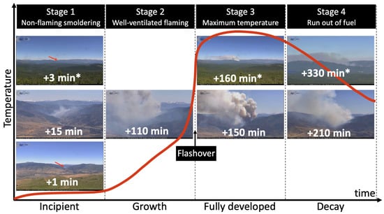 Figure 3. The 4 stages of fire. The example shown is the Farad Fire of July 2017 observed from two different cameras (Peavine fire camera and * Sage Hen Fire Camera).The definition of early detection is relative. In this paper, we define the early half of the incipient stage as early detection. Most studies consider the incipient and early growth stages as early detection [6]. However, through an inspection of numerous wildfire videos, we observed that wildfires at the growth stage commonly transition to fully developed very rapidly. For example, the Farad Fire in Figure 3 was confirmed around Minute 15, using fire cameras (i.e., the image at Minute 15 is zoomed in), and by the time the first suppression efforts were made, it was already at the brink of flashover (i.e., Minute 110). In densely populated California, the median detection latency is 15 min [11], typically reported by people calling 9-1-1. In the literature, only one study has explicitly focused on the incipient stage [11] and, in particular, earlier than 15 min. Unfortunately, their efforts have moved to the commercial side. Initially, we replicated their sliding window block-based detection model as the main baseline, but the accuracy of localizing smoke regions highly depends on the size and number of tiles (i.e., blocks), which made the inferences very slow. Thus, we opted for more advanced object detectors as alternative models, in particular Faster R-CNN [39] and RetinaNet [41], which have been successfully employed by recent work [16] for early wildfire detection.
 - Target objects: We noticed a trend that flame is correctly labeled as flame only when smoke is also considered as a separate target object.
- Object size and detection range are relative, based on the proportion of the object to the image size. We noticed that a majority of related works focus on close- and medium-range detection (i.e., middle or large relative object size), as listed in Table 1. In Figure 3, close range would be similar to the snapshot shown at +110 min and medium range to +15 and +330 min. Fewer studies have focused on far-range detection (e.g., +1 and +160 min). An example at Minute 3 shows the Farad Fire on the horizon.
3. Data and Methods
In this section, we present our open-source Transformer-supercharged benchmark, namely the Nevada Smoke detection benchmark (Nemo). Nemo is an evolving collection of labeled datasets and state-of-the-art deep learning models for wildfire smoke detection and localization. We extracted frames containing smoke from 1073 videos from AlertWildfire [12] and, then, labeled them with the class and bounding box of the smoke regions. We created a single-class smoke dataset and a separate multi-class dataset for fine-grained smoke detection based on the perceived pixel density of the smoke regions. We adapted two popular two-stage object detectors (i.e., Faster R-CNN and RetinaNet) and a Transformer-based one-stage object detector (i.e., DETR) for wildfire smoke detection. Our preliminary results confirmed the inherent problem of false alarms in object detection. To overcome this, we created additional dataset configurations to explicitly add negative samples and reduce false alarms. Finally, a separate public database (HPWREN [13]) was used to test our employed model’s ability to detect fire within the early incipient stage. Our benchmark (dataset and wildfire smoke detectors) is available for public use [48].
3.1. Dataset
3.1.1. Data Source
In recent years, multi-institutional research projects such as Alert Wildfire [12] and the High Performance Wireless Research & Education Network (HPWREN) [13] have become the leading source of live and archived video footage and image snapshots of rural and remote wildland areas on the west coast of the United States. While the initial objectives of these university-led projects have been research areas such as seismology and geophysics, they have morphed into invaluable resources for cross-disciplinary research in wildfire management, as well as for fire fighters and public safety agencies in multiple states. The network-connected cameras particularly help in: (1) Discover/locate/verify fire ignition through continuous manual observation of camera feeds, (2) scaling allocated resources according to spread dynamics and severity, (3) persistent monitoring of fire behavior through containment and until its demise, and (4) help develop an evacuation strategy and support decision-making in case of firestorms. While the cameras, sensors, and available resources are effective for the latter three, the initial step, which is discovery, can be greatly improved with sophisticated deep-learning-based systems [11]. In this paper, we collaborated with The University of Nevada’s Seismological Laboratory (NSL) [94], which is one of the leading groups in the AlertWildfire consortium, along with the University of California San Diego (UCSD) and the University of Oregon (UO) [12].
3.1.2. Domain-Specific Challenges in Camera-Based Wildfire Data
In this paper, our main wildfire object of interest is smoke, in particular smoke at the early incipient stage. To design an effective wildfire detection model, domain-specific challenges considering camera feeds, similar wildfire objects, and other factors related to non-object (non-smoke) classes need to be considered. Figure 4 shows an overview representative example of these objects.
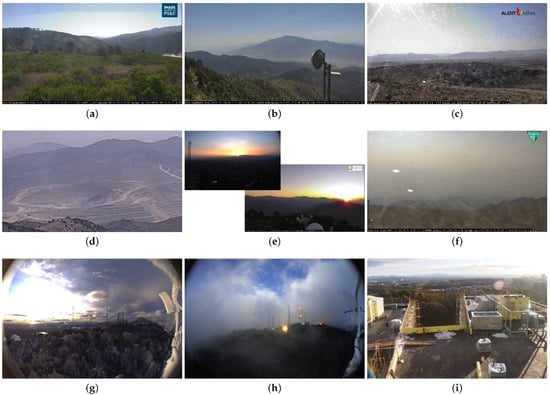
Figure 4.
Examples of smoke-like objects. Most images are from Nevada and California wildlands and the Sierra Mountains. (a) Small cloud on the right. (b) Cloud on a mountain top with hazy background. (c) Dirty lens, reflection, and smog. (d) Small pile of dust resembles smoke at an early stage. (e) Sunset and sunrise. (f) Heavy dust, glare, and smudge. (g) Tiny, low-altitude cloud, and snow. (h) Heavy fog and yellow flood light. (i) Miscellaneous objects and glare.
AlertWildFire [12] provides access to 900 cameras across eight states (i.e., Nevada, California, Oregon, Washington, Utah, Idaho, Colorado, and recently Montana). Such an expansion has been made possible due to the usage of existing communications platforms such as third-party microwave towers, which are typically placed on mountaintops. The camera placements offer an extensive vantage point with range views of up to 50 miles, which makes it possible to detect wildfires across counties. The extensive views from our source cameras pose unique challenges for object detection, as there will be huge backgrounds and the target object can be an excessively small portion of the frame, which causes an extreme foreground–background class imbalance. For instance, some of the images from our test set are from fixed wide-angle cameras that generate 3072 by 2048-pixel frames every minute. Consider the example shown in Figure 2: even with spatial clues such as our correct prediction, it is still difficult to see the smoke without zooming due to the extremely small relative size of the object compared to the background, which is less than 0.01% of the image in this case.
The background can include objects that are very similar to smoke or similar to objects that typically occur close or next to smoke (e.g., flame), which can also trigger false alarms. Furthermore, it is important to distinguish wildfire at advanced stages, which is larger and more distinctive and thus less similar to background objects and easier to detect. Most of these challenges only apply to smoke at the early incipient stage. According to our observations of numerous images, similar objects to incipient wildfire smoke include, but are not limited to: cloud, fog, smog, dust, lens smudge, snow, glare, and miscellaneous distant landscape objects such as winding roads, while similar objects to flame include the Sun and various shades and reflections of the sunrise and sunset.
3.1.3. Data Collection and Annotation
Collecting and labeling wildfire smoke from our raw videos came with certain challenges: small object size, the shallow and fuzzy nature of smoke, huge backgrounds and variety of smoke-like objects, unstructured and variable-length source videos, moving background scenes, obstruction caused by sunlight, glare, illumination, fog, haze, and other random environmental and technical factors that hamper visibility. We mainly overcame these challenges by careful and repetitive manual observation of the source videos with attention to spatial and temporal clues within the file names. Moreover, finding wildfire starts and labeling smoke objects at the early incipient stage is uniquely challenging and in stark contrast to the effort required for the later stages. Fine-grained relabeling of smoke objects based on their density also added to these challenges. To summarize, Figure 5 shows the preprocessing workflow for the early incipient stage. A group of individuals helped with this process, which took a substantial amount of time and effort in the form of revisions and re-annotations.
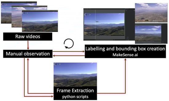
Figure 5.
Early incipient data preprocessing workflow. Raw videos are manually observed to determine the appropriate period for data extraction, using automated scripts. This is particularly necessary for long videos. The extracted images are then labeled with bounding boxes using the makesense.ai tool [95]. Since smoke at this stage tends to be small and typically not or hardly visible, a continuous feedback loop is crucial to locate smoke and draw the bounding boxes correctly. Finding wildfire starts is particularly difficult, since they are shallow and typically on or near the horizon.
We collected and annotated our data in different phases:
- Phase 1: initial frame extraction;
- Phase 2: single-class annotation;
- Phase 3: smoke sub-class density re-annotation;
- Phase 4: collage images and dummy annotations.
In the first phase, we closely inspected raw input videos and extracted the frames containing smoke objects. We then annotated the smoke objects with bounding boxes in Phase 2. In Phase 3, smoke instances were divided into multiple bounding boxes and relabeled based on the density of smoke pixels. We randomly divided our dataset into two non-overlapping sets (i.e., training and validation). We also handpicked a small test set of negative samples, consisting of challenging smoke-like objects. We then trained our deep learning models using the single-class and multi-class datasets. The initial results showed high accuracy with 1.2–2.4% of false alarms for the validation set. However, the models detected a relatively high number of false alarms in the challenging negative set. This motivated Phase 4, where we add new dataset configurations to increase the diversity of background objects. Table 2 provides an overview of our dataset configurations. The details of each phase are provided in the following.
Table 2.
Dataset configurations’ overview.
Phase 1—initial frame extraction: We use 1073 raw videos containing fires, acquired by our collaborators at AlertWildfire [12]. The acquisition system is based on pan–tilt–zoom (PTZ) cameras. The majority of fires happen in wildlands, forests, remote areas, or near highways. There are also residential fires, prescribed burns, car and plane accidents, and wildfires at night time. The video file names are unstructured and have no consistent or standard meta data and naming convention. Thus, reliably grouping them based on location, date, or other contextual information such as stage of development was not feasible.
Our extracted frames arefrom different stages of fire, as illustrated in Figure 3. We used spatial and temporal clues in the video file names to help extract more images from videos containing wildfire starts and the early incipient stage (e.g., Small Fire near Highway 40 (Mogul Verdi) put out quickly and Evans Fire starts at 744 AM and camera points at Peavine 833 AM) and less from videos containing advanced stages. The clues within the file names are crucial, as some of the fires were excessively small and very difficult to spot, even after zooming into high-definition snapshots, and sometimes even if the exact start time was known. The observation difficulty is usually due to smoke size, opacity, distance, weather, or lighting conditions, among other things. Moreover, the PTZ cameras are regularly zoomed and moved around after fire discovery. Thus, we tried to collect more frames before discovery. Due to the challenges above, we went through several iterations and re-annotations to make sure smoke regions are captured correctly. There are also videos that only show fully developed wildfires (e.g., Fire fighters turn the corner on the Slide fire, as seen from Snow Valley Peak at 4 PM and 5th hour of the Truckee Fire near Nixon, NV from the Virginia Peak fire camera 9–10 AM). Such footage are of no interest to us as there are no useful frames in the entire video. In total, we extracted 7023 frames and annotated 4347 images. However, many of these annotations were later removed from our dataset for reasons mentioned next.
Phase 2—single-class annotation: We initially annotated 4347 images using MakeSense AI [95], resulting in 4801 instances (i.e., smoke objects annotated with bounding boxes). At first, our annotations contained four classes: smoke, fire, flame, and nightSmoke, but we decided to only keep the smoke class. Determining the boundaries of smoke objects at night is a very difficult task with unreliable annotations. Flame is typically visible in the zoomed frames and more advanced stages, which is not our objective. The fire class, which we used to label bigger (typically more advanced) fires, was mostly removed or relabeled as smoke. What remained is our initial single-class smoke dataset containing 2587 images. It is randomly divided into 2349 training images containing 2450 instances and 238 validation images containing 246 instances.
A long-term goal and aspiration of our project is to design a system that aids in climate prediction and determining the severity of wildfire smoke particles and other hazardous pollutants and emissions. We noticed that in any stage of a wildfire, smoke columns have varying opacity and density. Smoke at the earliest stages tends to be shallow and less severe than smoke at later stages. In some cases, different sub-regions of the same smoke column tend to have varying opacity. Thus, to aid in our goal of detecting smoke at the earliest stage and to design a proof-of-concept model for detecting the severity of pollutants, we defined three additional sub-classes of smoke based on their density: low, mid, and high.
Phase 3—smoke density re-annotation: We re-annotated the single-class smoke objects into three sub-classes based on perceived pixel density: low, mid, and high. Figure 6 shows four typical examples of redrawing the bounding boxes to reflect various density levels. For better visualization, smoke that was relatively bigger or zoomed in was chosen. This sub-categorization helps account for variations in visual appearance and fine-grained information of smoke columns. There were, however, several unique challenges.

Figure 6.
Examples of smoke density re-annotation. The left side shows our initial annotation with the single category “smoke” (bounding box denoted with white color). On the right side, the same images were re-annotated with smoke as the super-category, and “low” (blue), “mid” (pink), and “high” (red) as the categories based on the relative opacity of the smoke. (a) Axis-Bald-Mtn-CA 2018-06-21 13:34. (b) Axis-SouthForks 2019-08-22 11:49. (c) Axis-Bald-Mtn-CA Placerville 2017-07-20 15:07. (d) Axis-Bullion Briceburg fire 2019-10-06 14:48.
One of the hardest challenges in re-annotation is finding low-density parts of the smoke, as they tend to blend into the background or are extremely small. We noticed that the only way to properly annotate the low-density areas is to revisit the video sources and use the movement of the shallow parts to distinguish the bounding areas in the respective captured frames. An interesting example of such a case is shown in Figure 6b, where only a large coarse bounding box was created at first and labeled as smoke. However, as shown on the right side, we re-annotated the image into a combination of five low- and high-density smoke areas. Interestingly, in our initial coarse annotation, we overlooked two new fires that had just started slightly in front of the large column of smoke. These two new fires were caused by embers falling from the bigger fire. Embers can be very dangerous and travel far and unpredictably based on the weather and wind conditions. With re-annotation, the two new fires would receive their own boxes with the appropriate density label.
Another challenge is to decide what constitutes different levels of density. The sub-categorization was performed subjectively, based on the relative opacity of different parts of the smoke column in the context of the background. We first attempted to automate the sub-categorization process, using relative pixel values and clustering algorithms to determine clusters of similarly colored grey-scales in different areas of the image. However, the camera feeds were captured at varying locations and varying times of the day with dynamic tilting and zooming, causing the scene and illumination to change drastically. Moreover, the relative position of the Sun and pre-existing weather conditions create more uncertainty, which makes the clustering approach highly unreliable. Thus, we manually annotated the smoke density with attention to existing background conditions and clues from the file names.
It is also important to note that the bounding boxes for density could be very granular within each image. For example, an entire column of smoke that was simply labeled as smoke could now be annotated using several bounding boxes (e.g., up to 10 in some cases). As a result, we ended up with considerably more instances. In this phase, we extracted another 200 frames from the source videos, all from the incipient stage. Our re-annotated dataset had three classes of smoke, with 2564 images containing 3832 training instances and 250 images containing 420 validation instances.
Challenging negative test set: We handpicked a set of 100 images containing no smoke from various sources (i.e., AlertWildfire, HPWREN, Internet). Importantly, this is not a set of random empty images, but 100 images, carefully and deliberately selected, to challenge the predictions based on the resemblance to smoke objects in our training set and other environmental conditions that make smoke prediction unreliable (e.g., haze, dust, fog, glare).
Phase 4—collage images and dummy annotations: We created additional dataset configurations to improve the diversity of background objects in our training set. We incorporated empty images by adding collages of smoke and non-smoke images or adding empty images without annotations. We also created a version of our dataset that added empty images with dummy annotations. This hack is suitable for situations where the underlying object detection codebasedoes not support negative samples for training. The motivation for Phase 4 was our initial results, which showed a relatively high number of false alarms in our challenging negative test set, as discussed in more detail in Section 3.3. Additional details about the collages and dummy annotations are provided in Section 3.4.
3.2. Nemo: An Open-Source Transformer-Supercharged Benchmark for Fine-Grained Wildfire Smoke Detection
Nemo is an evolving collection of wildfire smoke and smoke density dataset configurations and object detection algorithms fine-tuned for wildfire smoke and fine-grained smoke density detection. In this paper, our main wildfire smoke detectors are based on Facebook’s DETR, while also providing models based on the powerful Faster R-CNN with feature pyramid networks and RetinaNet as alternative smoke detectors.
3.2.1. DETR Architecture
The architecture of DETR is shown in Figure 7. There are three reasons why we chose DETR as the main model. First, it is based on encoder–decoder Transformers where the self-attention mechanism of the encoder layer performs the global processing of information, which is superior to the inherently local convolutions of other modern detectors. This helps the model attend to the global context of the image and improve the detection accuracy. Second, DETR employs a decoder layer that supports parallel decoding of objects, whereas the original attention mechanism [96] uses autoregressive decoding with RNNs and thuscan only predict one element at a time. Last, but not least, DETR approaches the task of predicting a set of bounding boxes directly in an end-to-end fashion. This effectively removes the need for complicated handcrafted process of designing anchors and region proposals associated with modern single-stage (e.g., Yolo family) and two-stage (e.g., FRCNN family) object detectors.
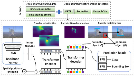
Figure 7.
Nemo overview.
The three main components of DETR are: a convolutional backbone, an encoder–decoder Transformer, and a feed-forward network (FFN) to predict the final detection output, as depicted in Figure 7. First, a CNN backbone (i.e., mainly Resnet50) extracts 2D feature representations of the input smoke image. The feature maps are then passed to the encoder in a flattened sequence, as expected by the encoder. A set of fixed sine spatial encodings is also passed as the input to each attention layer due to the permutation invariance of Transformers. The decoder, in turn, receives a fixed number of learned object queries, N, as input while also attending to the encoder outputs. Object queries are learned positional embeddings, and the model can only make as many detections as the number of object queries. Thus, N is set to be significantly larger than the typically expected number of objects in an image. In Nemo, we default to 10 and 20 object queries for single-class smoke and smoke density detection, respectively. Similar to the encoder, these object queries are added to the input of each attention layer, where the decoder transforms them into output embeddings. The output embeddings are then passed to the FFN prediction heads, where a shared three-layer perceptron either predicts a detection (a class and bounding box) or a special “no-object” class.
3.2.2. DETR Prediction Loss
The main learning brain of DETR is the bipartite matching loss. Consider a simple example with a ground truth image containing two smoke objects. Let denote the set of ground truth objects (i.e., class and bounding box pairs) and object queries; thus, is a set of predictions. We also consider ground truth y to be of size N. In this example, since there are only two ground truth objects in the image, we pad the rest (i.e., eight) with ⌀ (no smoke object). For each element i of the ground truth , we have as the target class label (e.g., smoke; low, mid, high, or ⌀) and in cxcywh format denoting the center coordinates, width, and height of the ground truth box normalized over the image size. Consequently, for each predicted box , we have an array of class probabilities equal to the number of categories plus one for the no-object class and predicted bounding box . Now, the two sets are ready for a bipartite matching search for a permutation of N pairs with the lowest pairwise matching cost as follows:
For all N pairs matched in the previous step, the overall loss is efficiently computed using the Hungarian algorithm [47]. Similar to common object detectors, the loss is defined as a linear combination of class loss and box loss. The class loss is the negative log-likelihood, while the box loss itself is a combination of the commonly used loss and generalized IoU loss [97].
3.3. Inherent False Alarm and Class Imbalance
Our preliminary results on single-class and multi-class smoke density detection showed promising performance, as in Table 3. Especially for the single-class model, our results are comparable to official DETR evaluations on the COCO dataset based on mAP. This is interesting given that the official models have seen upwards of 11,000 images per target class on average, compared to 2500 smoke images in our case. This confirms that transferring weights from a model trained on different everyday objects and retraining the classification head for smoke detection is promising.
Table 3.
Preliminary results (in percentage (%)). False positive rates are marked in bold. FPR is the false positive rate for the validation set consisting of images containing smoke. FPR is the false positive rate for the challenging negative test set.
Figure 8 illustrates examples of smoke detection from the models presented in Table 3. Through extensive visual inferences and numerical evaluations, we confirmed the high accuracy of our wildfire smoke detectors. In particular, smoke was detected and localized in positive images with great precision and rare false positives, as noted by the 1.2% false positive rate (i.e., FPR). However, testing against our challenging set of empty images resulted in a false detection, as highlighted in Table 3 under FPR. This motivated us to investigate whether the false alarm issue is due to our training or the inherent performance of the base model (i.e., DETR trained on COCO) that we transferred the weights from. To confirm this, we conducted the following two evaluation experiments.
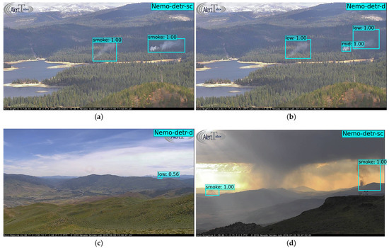
Figure 8.
Representative examples of smoke detection from the models presented in Table 3. (a,b) show single-class and density inferences, respectively, of the same image: prescribed burns near Union Valley Reservoir seen from Big Hill Mtn, CA. (c) Sage Hen incident north of Truckee, CA. (d) Tule and Rock fire take off northwest of Virginia Peak, CA.
First, we qualitatively evaluated the base model against challenging images containing the desired COCO objects, similar to the example shown in Figure A1. The full list of COCO classes is available online [98]. We verified that the base model has exceptional detection performance, which was expected and in line with the results reported in the paper [47].
Second, we tested COCO DETR against our handpicked negative test set, which includes smoke-like objects. Besides a few exceptions (e.g., person, airplane, and truck in the background), this set does not include any of the 80 COCO objects. Our tests, shown in Table 4 under FPR, returned false detections, meaning DETR classified background objects incorrectly in 20 different images out of 100. Note that we did not handpick this test set for similarity to COCO objects (e.g., cauliflower to resemble broccoli, etc.), so our test set is relatively easier for a COCO detector, compared with a smoke detector. Furthermore, the original DETR is trained on COCO 2017 dataset, which has a higher number of objects and variety for each target class. This exploratory test confirmed that the false alarm performance of our wildfire smoke detection is inherent from the base transferred model. Through numerous visual tests, we confirmed that in the presence of desired objects, the detector is accurate and precise, even in the presence of challenging target-like objects (Figure 8). However, in the absolute absence of target objects, the model tends to predict false alarms on target-like objects in the background. This could be intuitively understood as the attention mechanism of the Transformer model is designed to focus on the target object, making the model robust against the target-like objects in the background when there exists a target object. Figure 9 shows examples of false alarms created by our single-class and density smoke detectors alongside inferences from DETR’s COCO object detector. This offers a visualization of our previous discussion.
Table 4.
Evaluation of DETR models on the COCO validation set (denoted by the mAP) and false alarm performance against images with no target objects (denoted by the FPR). We mainly transferred weights from DETR with 42% AP on the COCO benchmark. This shows that even the highest-performing object detector with a state-of-the-art 44.9% mAP still creates 15 false alarms when used against images with no COCO object. This shows that our smoke detector with 21 false alarms against a dataset with smoke-like objects is already performing well and as expected.
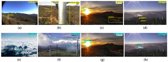
Figure 9.
Images on the top show false alarm examples of the DETR COCO detector on our challenging non-object test set. Images at the bottom show the same, but for the Nemo-DETR models presented in Table 3. (a) A tall tree is detected as a giraffe. (b) A camera attached to a pole is detected as an airplane with 99% confidence. (c) A driveway is detected as a boat. (d) Glares are detected as kites with high confidence. (e) Cloud in an unrealistic background detected as medium density smoke. (f) Rainy cloud detected as smoke. (g) Sun is detected as smoke, based on the similarity to flame, which is an object that exists near smoke in some training images. (h) Fog is detected as high-density smoke.
Image classification focuses solely on correct classification of images, whereas object detection involves both classification and localization of objects within images. Unlike image classifiers that explicitly feed negative samples to the model, object detectors are typically trained with positive images and their respective bounding box annotations, and the negative samples exist implicitly, meaning all regions of images that do not correspond to a bounding box are “negative samples”, which by itself is the clear majority of the data. In fact, a well-known problem in object detection is extreme foreground background class imbalance, where easily classified negatives can degenerate training by dominating the loss. To counter the class imbalance, an effective approach is to down-weight easy negatives. In our adopted models, Faster R-CNN uses subsampling to balance positive/negative region proposals. For RetinaNet, focal loss (FL) [41] is employed as in Equation (3) to down-weight the easily classified samples.
where is a modulating factor with a tunable focusing parameter , which controls the rate of down-weighting easily classified samples. Consequently, if is 0, then FL would be the same as cross-entropy. Empirically, has been found to work best, but given the different nature of smoke object detection, we experimented with different values and found no significant differences, so we opted for the default.
For our main adopted model, DETR [47], we use a coefficient to down-weight the log probability term when the class is predicted as non-object (i.e., background) in the bipartite matching loss, as specified in Equation (2). By default, we down-weight easy negatives by a factor of 10, but other values were extensively tested. Despite using these methods for tuning the down-weighting parameters, the false alarms reported in Table 3 and Table 4 still need to be improved.
3.4. Collage Images and Dummy Annotations
To improve our preliminary models in terms of false alarms, we incorporated empty images (i.e., images with no smoke, all background) using different strategies: simply adding empty images with no corresponding annotations, creating and adding collages of smoke and empty images with their respective bounding box annotations, and finally, adding empty images with dummy category annotations.
Given the inherent problem of the extreme foreground background class imbalance discussed earlier, adding more background in the form of empty images seems counterintuitive, as it increases these problematic easy negatives in our dataset, making the extreme imbalance even more extreme. We argue several reasons and discussion points on why it may be necessary to add empty images explicitly.
Single-stage object detectors, such as DETR, do not refine the proposed bounding boxes, using a complementary classifier, or nonmax suppression. The fact that DETR outperforms two-stage detectors on the challenging COCO benchmark simply attests to the superiority of Transformers. However, to further improve its robustness against challenging backgrounds in the wildfire domain, it is important to improve the diversity of the non-smoke background.
One obvious and the most effective way would be to collect enough positive data to cover a reasonable variety of backgrounds, which is a very challenging task, especially for wildfire smoke in the early stages. Target objects do not always happen with all possible backgrounds. For example, in our initial training set (sc and d), we do not have smoke happening in the same image as different shades of sunrise and sunset. Consequently, our initial model tends to incorrectly detect Sun as a smoke object, as shown in Figure 9g. The same situation applies to snow as wildfires amid snow are rare, but possible [99]. Thus, it is important to diversify the background, and one way of doing so is by adding empty images to the dataset with no bounding box annotations.
Object detection algorithms were not originally designed with the expectation of adding explicit negative samples. In fact, support for negative samples was only added recently. For instance, Faster R-CNN and RetinaNet did not support negative samples until April 2020 (i.e., PyTorch v0.6.0) and March 2021 (i.e., v0.9.0) updates, respectively [100]. Thus, the code base for many existing inference systems may not support negative samples. Therefore, to cover such scenarios, we tried two workarounds: one harder, but robust approach (collages) and another easy, scalable, but hacky approach (dummy annotations).
3.4.1. Collages
The first approach is using combined images (i.e., collages) of smoke and non-smoke scenes, similar to Figure 10. However, creating such collages and annotating smoke objects requires significant effort. First, collages need to be created in a way that avoids the introduction of spatial bias to the model. For example, the non-object and object images should not dominantly be in the same position within the collage (i.e., top-right, top-left, etc.), but shifted around in different ways to add variety. For instance, Figure 10a,b are permutations of the same set of images, some containing smoke and some only smoke-like background. Once collages are created, bounding boxes must be manually drawn and labeled, which can be laborious, given that the smoke sub-images may contain incipient smoke that is much smaller compared to the full images. To annotate the bounding boxes in some of the collage images containing small smoke objects, we employed our existing detectors to help us find smoke regions, albeit not always reliable.
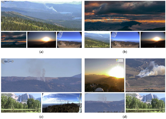
Figure 10.
Four representative examples of collage images used for training. Different configurations were used (e.g., 1 by 1, 1 by 2, 2 by 1, 2 by 2, 1 by 3, etc.). The images within the collages were often reused, but shifted to create variability and avoid learning bias. (a,b) are permutations of the same set of images. In (a), the bottom-right and top images have smoke, and the other images are used as new background samples. (c) Collage of three images, with a larger image containing smoke and two smaller images containing non-smoke background. (d) The top-right and bottom-left are images containing smoke, and the top-left is a shade of sunrise that our initial training had never seen due to a lack of incipient-stage smoke happening naturally in such a background.
The multi-step and time-consuming task of creating and annotating collages meant that we settled for 116 of these collages to add to our training set, as also specified in Table 2. The number of added collage images may not be enough, but in practice, the collages would add background variety and positive samples at the same time, thus affecting class imbalance less than simply adding empty images. The difficulties of creating collages prompted us to think of another work-around, a simpler one.
3.4.2. Annotations with Dummy Category
The second approach is to add empty images directly (no collage) and add a dummy class. Then, for each empty image added to the dataset, create a minimal bounding box (1 by 1 pixel) with a random location within the image dimension. The advantage of this approach over creating collages is that it can be easily automated and scaled up in seconds, as it does not need any manual annotation of smoke objects. We created a simple pipeline to obtain empty images, extract their dimensions, and then, generate a random bbox with COCO format as follows:
where rand(0, Width) and rand(0, Height) create random top-left x and y positions, respectively, within the image dimension. The bounding boxes have the minimal width and height of 1 pixel. Random positioning of the dummy object is crucial, as the model would learn unimportant features, if for instance, a fixed position of top-left (i.e., 0, 0) was chosen based on the assumption that no target objects are at those extreme locations. Consequently, during inference, any detection of the dummy category would be discarded. This work-around would support older object detection inference systems that do no support negative samples.
To cover all configurations, we consider the option of adding empty images without the corresponding entry under the annotations in the COCO format. In conclusion, we tried all configurations to cover any scenario where the object detection algorithm did or did not support images with no annotation entry. Table 2 lists our dataset configurations. For single-class annotation, we do not attempt dummy or collage annotations and leave other configurations for future exploration. In the next section, we present the full evaluation results, including our baselines, RetinaNet, and Faster R-CNN, which we trained with our dataset for comparison.
4. Experimental Results and Discussion
In this section, the full comparative evaluations are presented based on the metrics presented in the following section.
4.1. Performance Evaluation
To evaluate the performance of our models, we used various metrics. For consistency, we mainly focused on the Microsoft COCO criteria and Pascal VOC metric, as in Table 5, all of which are based on the intersection over union (IoU), while using other metrics to further evaluate our density detectors. The IoU is commonly used to evaluate object detection algorithms. It measures the overlap between the predicted bounding boxes and the associated ground truth boxes via the following Equation (4).
Table 5.
COCO evaluation criteria.
A perfectly overlapping prediction would get an IoU score of 1, while a false alarm (i.e., predicted bounding box with no overlap) gets a zero. Consequently, the IoU can be used to determine whether the predicted bounding box is true or false by setting a fixed threshold for the IoU. If the IoU is bigger than the threshold, the detection is considered to be correct; otherwise, the detection is considered false and discarded.
However, a fixed threshold can potentially cause bias in the evaluation metric. Thus, it is common to use the Microsoft COCO mean average precision (i.e., mAP, or simply AP) as the primary metric to evaluate object detection algorithms. The AP interpolates 10 points associated with 10 different thresholds in the 0.5–0.95 range with a step size of 0.05, as specified in Equation (5).
Based on the above, the COCO evaluator (i.e., pycocotools [101]) automatically measures the AP at different levels and scales, as mentioned in Table 5. The IoU score of 0.33 was also considered, inspired by a recent study [16], which specifies smoke objects to have a fuzzy appearance, and lowering the overlap threshold would help keep valid smoke detections that otherwise would be discarded.
Besides the standard MS COCO and PASCAL VOC, we define separate metrics to better evaluate our models, especially for models trained on our smoke density annotations. Smoke is a special object, with diverse shapes and patterns [10]. As mentioned in smoke density re-annotation (see Section 3.1.3), breaking a single columnof smoke into fine-grained sub-regions based on density can result in drawing and labeling inconsistencies, and noise in data (Figure A2). Thus, bounding boxes generated by smoke detectors may be slightly misplaced from the ground truth and impact the AP results, but the detectors do identify the regions successfully, as shown in Figure A2. In addition, the inherent similarity between our neighboring density classes (i.e., low vs. mid and mid vs. high) can also impact the AP results. Importantly, a case where the prediction is two density levels off is rare in our results, especially for Nemo-DETR. Moreover, with the extremely small smoke objects (i.e., ∼ pixels), the smallest shift in the predicted bounding box relative to the ground truth can drastically affect the overlap and the corresponding IoU. Inspired by [10] and to evaluate the models more comprehensively, we use two additional metrics: frame accuracy (FA) and false positive rate (FPR). For a positive image, if the detector misses any smoke object, we count it as a frame miss (FM), otherwise as a frame hit (FH). Consequently, if the detector predicts any smoke-like object in our challenging negative set as smoke, we count it as a false positive (FP), otherwise as a true negative (TN). We then calculate the as specified in Equation (6):
4.2. Results
In this section, we present the complete comparative evaluation of our smoke object detectors (i.e., FRCNN, RetinaNet, and DETR). It is important to note that FRCNN and RetinaNet have been used before for wildfire detection and, very recently, fine-tuned by [16] to achieve impressive results. Their dataset is similar in terms of the number of images. Their training data were collected from national parks in Portugal, while ours from Nevada and California, which are relatively similar. However, due to some commercial aspects of the existing work [16] and the fact that we use different datasets, we do not compare them directly for evaluation. Instead, we trained Faster R-CNN and RetinaNet with our datasets as the reference for comparison. Table 6 and Table 7 list the detailed comparative evaluation of the Nemo smoke and smoke density detectors, respectively. Figure 11 and Figure 12 show an example of smoke bounding box detection for the single-class and density detectors, respectively. The employed models were trained using different Nemo dataset configurations, as noted in the name according to Table 2. Despite performing extensive experiments with different hyperparameters, we only include results from select model checkpoints with the highest mAP for consistency and brevity. The models and datasets are available at project Nemo’s GitHub [48] along with more details about the experiments.
Table 6.
Wildfire smoke detection results. Three different models, DETR, FRCNN, and RetinaNet (RNet) were trained with our dataset (Nemo) using the two data configurations from Table 2 (sc and sce).
Table 7.
Wildfire smoke density detection results. Wildfire smoke detection results. Three different models, DETR, FRCNN, and RetinaNet (RNet) were trained with our dataset (Nemo) using the data configurations from Table 2 (d, dg, de, dge, and dda).
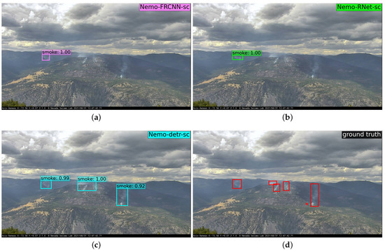
Figure 11.
Wildfire single-class smoke bounding box predictions by (a) Faster R-CNN (Nemo-FRCNN-sc), (b) RetinaNet (Nemo-RNet-sc), and (c) DETR (Nemo-DETR-sc). (d) shows the ground truth annotation. The image shown is from a camera at Aeneas Lookout, Washington, 31 August 2021.
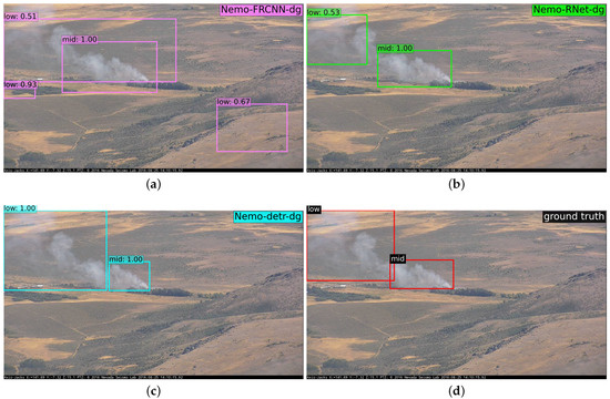
Figure 12.
Wildfire smoke density bounding box predictions by (a) Faster R-CNN (Nemo-FRCNN-dg), (b) RetinaNet (Nemo-RNet-dg), and (c) DETR (Nemo-DETR-dg). (d) shows the ground truth annotation. The image shown was recorded August 2016 from the Axis-Jacks camera located at Jacks Peak, Northern Nevada.
The results confirm that improving the variety of background using any of the strategies (i.e., collage, empty images with and without dummy annotations) can significantly reduce the number of false positives in our challenging negative set, as denoted by FPR. Importantly, however, the overall performance and precision of smoke bounding box detection is not significantly improved for positive images, as specified by mAP. For example, the best initial single-class model in terms of mAP returned 26 false alarms in our challenging non-smoke dataset, while after adding empty images, the number of false alarms significantly dropped to three. However, the mAP and PASCAL VOC metric (AP50) did not significantly improve. For instance, the mAP is only improved by up to 1.7% and 0.4% for smoke and smoke density detection, respectively. The same observations apply to RetinaNet and Faster R-CNN. We hypothesize this to be due to the extra class imbalance introduced by adding empty images, further diluting the loss. We also notice that the models trained with collage images (dg) returned the highest average precision for DETR and RetinaNet and the second-highest for FRCNN, which is interesting because collage is the only data configuration besides original (i.e., sc and d) that does not add significant class imbalance to the dataset.
The main advantage of adding empty images, compared to collages, is simplicity. However, the downside of adding empty images, regardless of whether the annotation of those images is added using a dummy category or not, is that the extra class imbalance may require negative class down-weighting to be revised. However, there are empirically found upper-bounds for how much to down-weight the background and not sacrifice the detection rate and accuracy. After all, the model also needs to learn the negative samples, and there is a limit to which they can be down-weighted. These limits have been empirically found by the literature [41,47]. We also tested different values to down-wight the easy negatives and found that the default values work best with insignificant anomalies. We also experimented with different numbers of added empty images and noticed that, beyond the numbers reported in our dataset overview in Table 2 (i.e., 260), adding more empty images do not necessarily improve the overall performance, as it would simply add more class imbalance and require us to tune the down-weighting, which in turn would sacrifice the performance in other aspects. Thus, the long-term solution for improving the accuracy in deep-learning-based object detection methods is always adding more positive data.
Moreover, the results show that models based on DETR can detect smoke regions correctly in up to 98.4% and 93.6% of the validation frames for the single-class and density detectors, respectively. This is while most models based on FRCNN and RetinaNet also achieve a high frame accuracy (i.e., up to 86.4% and 78.8% for the single-class and density detectors, respectively). The primary challenge metric, mAP, also shows a significant advantage of the models based on Transformers.
In Table 7, the smoke density results based on COCO metrics are misleadingly low for all models, as AP is directly affected by slight misclassification of density classes (e.g., detecting high as medium density). Additionally, the ground truth bounding box annotations can be very granular and cause the COCO validations to suffer, even when the actual predictions are sound. Figure A2 shows additional examples for smoke density detection and their respective ground truth. The figure shows the ability of the density detector in localizing the smoke and determining the density with acceptable accuracy (i.e., worst case of one density level from the ground truth).
4.3. Early Incipient Time-Series
In this section, we evaluate the performance of our smoke detectors in the early incipient stage. For this purpose, video sequences from the incipient stage of 95 wildfires were extracted from the HPWREN public database [13]. HPWREN provides a temporal sequence of images before and after fire ignitions in 1-minute intervals. First, we used 16 specific video sequences that were used in a similar time-series analysis by Guedes-Fernandez et al. [16]. Furthermore, we extracted 79 additional wildfire sequences from 1660 HPWREN images processed by Govil et al. [11].
The choice of these independent datasets is particularly interesting for two reasons. First, our model was trained and validated mainly on PTZ cameras that are typically 2 Mega Pixels. However, the HPWREN images are from fixed lookout systems with much wider range and are typically 6 MP in size, which is much larger than what our models have seen. These differences would challenge the generalizability of our trained models. Moreover, the HPWREN cameras operate mainly in Southern California, whereas our models were trained on scenes from Nevada and Northern California and may contain different environments. Second, these images were collected only within the incipient stage of the fire. In particular, Govil et al. [11] collected the 1660 additional images with the goal of detecting wildfire smoke before 15 min from ignition. Thus, they are very appropriate to test our wildfire smoke detectors’ ability to detect smoke in the early incipient stage.
Previous work (Fire21’ by Guedes-Fernandez et al. [16]) has evaluated the detection time of their best- and worst-performing smoke detectors using the 16 sequences listed in Table 8. Their smoke detectors are based on FRCNN and RetinaNet. It is important to note that we also trained FRCNN and RetinaNet on our dataset, but for a better evaluation, we used the best results reported in [16] for the 16 sequences. In addition, 79 more sequences were added to this study and analyzed using our FRCNN and RetinaNet models.
Table 8.
Incipient stage first smoke detection analysis. Sixteen smoke sequences extracted from the HPWREN database [17] and 79 sequences extracted from a collection of HPWREN images [102]. The earliest detection for each case study is marked in bold.
Table 8 shows the time elapsed from the start of the fire until the first correct detection of smoke. For brevity, we used the single-class smoke detector (i.e., Nemo-detr-sc) with a 41.2% reported AP and the collage-based smoke density detector (i.e., Nemo-detr-dg) to obtain these results. The detection times listed under Fire21’ (Guedes-Fernandez [16]) are from the best-performing model in their study (i.e., Faster R-CNN + FPN). They did not report the detection time analysis for their best-performing RetinaNet model. The first and second columns show the name and fire start time for each of the 16 video sequences from the HPWREN fire ignition database [17]. Importantly, the results reported in [16] were based on custom start times, defined by the authors, to account for the fact that, in most sequences, the frame associated with ignition (and a few frames after in some cases) has no visible smoke. We also confirmed this by carefully inspecting the video sequences. For this report, however, we used the original start times defined by HPWREN, which can be better for the repeatability and interpretability of the results. Consequently, the authors [16] kindly shared the information needed to convert their results to the same inference time.
The penultimate row of Table 8 shows the mean detection time for the first 16 sequences in common with [16]. The last row takes into account all 95 sequences. Since Nemo-DETR-sc and Nemo-DETR-dg performed very similarly for the first 16 sequences, we only used DETR-sc for the remaining 79 sequences. We list the incipient stage detection time for the additional 79 case studies in Appendix Table A1. For the 79 sequences, we used Nemo-FRCNN-sc and Nemo-RNet-sc. The results show that Nemo-DETR-sc perform better than FRCNN and RetinaNet. Across all 95 sequences, Nemo-DETR-sc detected smoke 4.2 s earlier than the next-best-performing model (i.e., Nemo-FRCNN-sc). This is also visualized in Figure 13.

Figure 13.
Cumulative detection rate vs. time elapsed after ignition. The Y-axis shows the cumulative percentage of the first correct detection within the X-axis minutes. The example marked in red shows that in 80% of the video sequences, DETR detected smoke correctly within 5 min from start of the incipient stage. 91.6% of the fires are detected within 8 min.
Figure 13 is derived using cumulative distribution function from the detection times of all 95 fire sequences. The graph shows that the DETR-based model detected 67.3% of the fires within 3 min, while 95.6% of the fires were detected in less than 15 min. This confirms the effectiveness of the DETR-based detector in the early incipient stage. Overall, Nemo-DETR-sc detected 97.9% of the 95 wildfire sequences within the incipient stage, while Nemo-FRCNN-sc and RNET-sc detected 68.4% and 54.7% of the wildfires within the incipient stage, respectively.
In Table A1, the data points marked as N.D. (i.e., not detected) are the ones where the model failed to detect smoke within the incipient stage. It is quite possible that the model eventually detect the smoke in a later stage of fire (e.g., growth stage), but we would not know as our analysis focused merely on evaluating the incipient stage. The 1660 frames used to obtain the additional 79 sequences are on average from the first 20 min of fire, which is the reason behind many of the N.D.s.
Finally, the missing data (N.D.s) can cause some unfairness in comparison of the models, since the mean is calculated over the reported detection times and not the missing data. We do not want to penalize the evaluation of a model that predicts smoke late, compared to another model that does not. For example, Row 53 from Table A1 shows that RetinaNet detected the smoke 32 min after ignition, whereas FRCNN failed. This particular case would largely increase RNet’s mean detection time, while not affecting FRCNN. Thus, for a balanced and fair comparison, we performed a simple imputation by substituting missing values (N.D.) with the neighboring extreme values from the successful model in each case study. For instance, in Row 53, the time reported for FRCNN (N.D.) would also be changed to the 32 reported by RNet for the same case. The results associated with the improved mean after imputation are shown in the row labeled as R3. Note that this change reduced the performance gap between the two models. In conclusion, it is important to look at the mean detection time in the context of the detection rate (R1). Overall, Nemo-DETR-sc failed only in two case studies to detect the smoke bounding boxes in the incipient stage. This translates to a 97.9% detection rate.
Figure 14 shows the three images from Table 8, where smoke was correctly detected after 8 min using Nemo-DETR-sc. For better visualization and due to the small size of the smoke, we removed the class label from some of the images. To investigate these relatively late detections, we looked at the prior frames leading up to the first detection and noticed a trend of smoke being both unusually small and shallow, thus blending into the background. In the case of Figure 14c, the smoke is not visible until 8 min after ignition, which contributed to the late detection. Figure 15 shows the images where smoke was detected the earliest, that is either at birth or 1 min later.
Figure 14.
(a) 20160722_FIRE_mw-e was taken on 22 July 2016 at 14:43. (b) 20170625_BBM_bm-n was taken on 25 June 2017 at 11:54. (c) 20180504_FIRE_smer-tcs8 was taken on 4 May 2018 at 14:41.
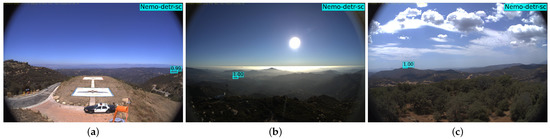
Figure 15.
(a) 69bravo-n was taken on 13 August 2019 at 14:20. This image shows the correct detection of smoke at the time of ignition. (b) 20200806_SpringsFire_lp-w was taken on 6 August 2020 at 18:34, and (c) 20180809_FIRE_mg-w was taken on 9 August 2018 at 13:10. This image as well shows the correct zero-frame smoke detection.
Detecting smoke columns that are extremely small and near the horizon is very challenging. As a representative example, Figure 16 shows the temporal sequence for sp-n-mobo-c__2019-07-28 (Row 72 of Table A1). For diversity, this inference is based on Nemo-DETR-dg. In this sequence, the first correct detection occurred 7 min after ignition. The frames associated with ignition, Minute 4 and Minute 7, with the correct prediction are shown. Due to the size of the smoke and bounding box covering the smoke, the zoomed-in version of the smoke region without the bounding box is also given for reference. We noticed that the smoke is barely visible in the first five images of the sequence and then gradually becomes larger. Due to the small size and the already smokey background, our best-performing model struggled to detect this fire earlier than the average mean time of 3.6 min.
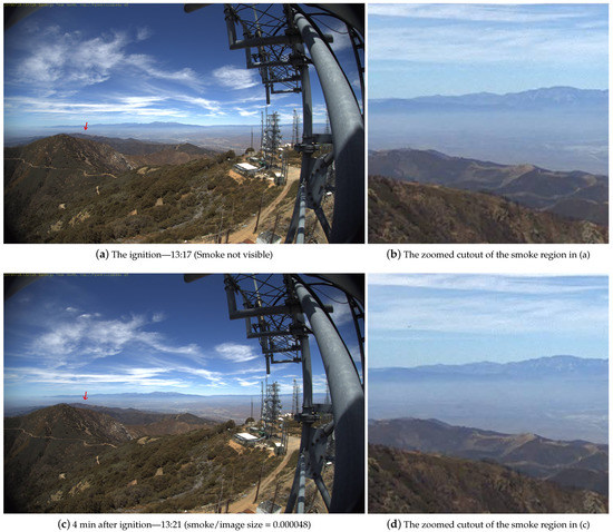

Figure 16.
The video sequence shown is from sp-n-mobo-c__2019-07-28 (Row 72). The images are 6 MP in size (i.e., 3072 × 2048) and were captured from a north-facing wide camera on top of Santiago Peak in Southern California. (a) shows the ignition at 13:17 marked with a red arrow due to the small size; (b) a 300 × 300 cutout of the ignition. We can notice that the smoke is not visible due to the small size, distance, and a background that is already smoggy. (c) A missed detection is shown 4 min after ignition at 13:21. The size of the smoke is 19 × 16 pixels, which is 0.0048% of the image (i.e., 3072 × 2048). (d) Note that the smoke is barely visible even in the 300 × 300 cutout. (e) The first correct detection is shown 7 min after ignition. The smoke is now 43 × 23 pixels, which is much larger than Minute 4, but still very small relative to the image dimension (0.01% of the image). (f) shows the cutout for the correctly detected smoke.
DETR does not rely on second-stage improvements. However, it still performs better than the state-of-the-art ConvNets. In Faster R-CNN, for instance, thousands of coarse region proposals (similar to the cutouts shown in Figure 16b,d,f) are fed to the second-stage classifiers and, then, to nonmax suppression for filtration and deduplication, but still, they did not detect the smoke in this example and many similar ones. We hypothesize that the superiority of the Transformer-based system is due to several encoder and decoder layers in which the perfect memory of the self- and inter-attention mechanisms helps narrow the attention of the model towards finer details after each layer. Moreover, even before the decoder attempts to extract the objects and make predictions, the layers of the encoder self-attention have simplified the task for the decoder by making some sort of instance separation.
5. Discussions
From Table 6 and Table 7, we conclude that Nemo-DETR outperforms the Faster R-CNN and RetinaNet variants. This was expected based on the COCO results reported in the DETR paper [47], but our results confirm that Transformer-based object detection is superior for smoke detection as well. In this section, we discussed why the attention mechanism and encoder–decoder Transformer used in Nemo can improve the performance.
5.1. Why Do Visual Transformers Work Better than State-of-the-Art ConvNets?
The self-attention mechanisms of the encoder help capture global-image-level relationships between the activations, which helps the model suppress duplicate predictions. The weights associated with the last encoder layer of our trained Nemo-DETR-dg model are shown in Figure 1. This shows how the model encodes the objects and already attends to a form of instance separation earlier in training and before the decoder phase. The global self-attention of the encoder is particularly vital for the better performance of DETR, compared to FRCNN and RNet, because it helps avoid near-identical boxes and the target-like object(s) in the background. It models pairwise relationships between all elements in the image and thus helps suppress duplicates without solely relying on post-processing steps, such as nonmax suppression (NMS). In contrast, the RPN proposals of Faster R- CNN tend to overlap, and a nonmax suppression mechanism is used during training to suppress the duplicates. Despite that, we applied additional nonmax suppression with an IoU threshold of 0.3 during the inference, which greatly improved the predictions. We applied the same inference time NMS to the Nemo-DETR visualizations for consistency. However, through extensive comparison with the inferences without NMS, we confirmed that the Nemo-DETR models were not as improved as the baselines. This is in line with what was reported in the DETR paper [47], where, with six decoder layers, the improvement provided by NMS was insignificant. This is due to the self-attention mechanisms over the activations in subsequent layers, which help remove near-duplicate predictions without relying on nonmax suppression.
To further understand the importance of the encoder self-attention mechanism, we performed a simple ablation study by removing encoder layers with a constant number of decoder layers. For reference, we used the single-class model (NEMO-DETR-sc) with a reported 40.6 mAP and the default 6 encoder and 6 decoder layers. Table 9 shows the ablation results for the number of encoder layers.
Table 9.
Ablation analysis for encoder size. Performance gradually improves with more encoder layers.
As specified in Table 9, with no encoder layers, the AP reduced by 6.3 points, with the most significant drop for small objects. We also tried using more than six attention layers, but training was expensive in terms of the schedule and resources, while the improvements were insignificant.
Moreover, the attention mechanisms of the decoder layers are key components that capture pairwise relations between feature representations of different object predictions. To better understand how the model detects smoke regions in different parts of the image, we visualize the encoder–decoder multi-head attention weights of the last decoder layer in Figure 17. Intuitively, this corresponds to visualizing, for each detected object, which part of the image the model was looking at to predict this specific bounding box and class. For brevity and simplicity, we only used models trained on the sc and d dataset configurations.
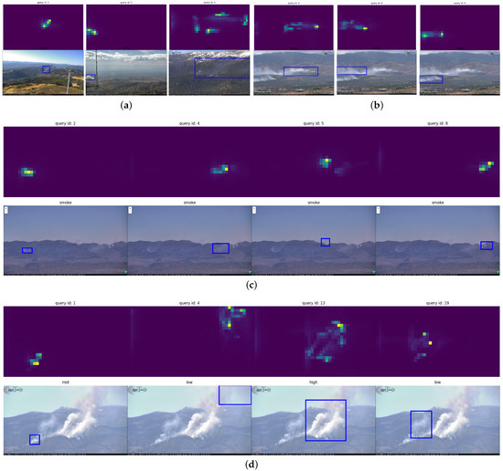
Figure 17.
Representative examples of wildfire smoke predictions (lower images) and visualization of the decoder inter-attention for each prediction (upper image). Predictions were made with the base Nemo-DETR-sc and Nemo-DETR-d. The respective attention weights at the last decoder layer in the top part of each image show where in the image the model (i.e., object query) was looking at to predict each specific bounding box and class. This visualizes the effectiveness of attention-based models in finding smoke regions. (a) Smoke correctly detected in 3 different images. (b) Hawken fire: 3 smoke regions detected in 1 image. (c) Little Den fire, 4 small fires detected in 1 image. Each prediction is denoted with its associated bounding box (lower image) and encoder–decoder multi-head attention weights (upper image). (d) Example of smoke density prediction. Each predicted box is shown separately with the associated attention weight. Each object query has a predicted a bounding box, and their density was correctly determined.
5.2. Limitations and Future Work
The images used in Section 4.3 are from entirely different databases and locations, compared to our training set, which attests to the generalizability of our method. However, the biggest limitation of our study still remains the dataset, for multiple reasons. First, we did not consider night-time wildfire smoke detection, which is crucial, since nearly 85% of wildfires are caused by humans [103], some from activities that may start fires during the night (e.g., unattended campfires, intentional act of arson). It is important to distinguish between flame detection and smoke detection. Flame detection during the night is a relatively simple task due to the sharp features of the flame and its contrast in the night background, and it has been extensively studied in the literature (Table 1). However, finding and annotating bounding boxes of wildfire smoke during the early phases are very challenging, even for the daytime case. The smoke in the early minutes of a wildfire is barely visible during the daytime (e.g., as shown in Figure 15 and Figure 16), let alone during the night. A carefully processed and annotated night-time dataset for smoke bounding box detection can therefore greatly improve the existing models. Nemo is an evolving benchmark, and we plan to increase its scope in terms of the datasets and deep-learning-based object detectors used.
Second, despite using dataset variations to include empty images of smoke-like objects and significantly reducing false detections (as shown in Table 7), false positives remain an inherent part of object detection. Furthermore, by injecting empty images during training of object detectors, we intentionally increase the already problematic foreground background class imbalance, which then requires additional effort and tuning to avoid sacrificing detection rate. Thus, the proper long-term solution would still be to increase the variety of positive data in different backgrounds, which demands significant effort by the community. In Nemo, we plan to regularly expand the dataset and retrain our select best-performing models. Figure 18 shows a few examples of smoke-like objects incorrectly identified as smoke. These images are from our handpicked test set of negative examples. Even though the models trained on collages and empty images produced significantly fewer false alarms, there are still few cases in poor environmental conditions, such as haze and dust.

Figure 18.
(a) Detection of cloud as smoke in an uncommon background for wildfire scenarios. All three false alarms created by Nemo-DETR-sce are of these kinds (professional nature photography). (b) San Juan hills south, a location not seen by our models. A white flat building near the horizon is incorrectly detected as low-density smoke. The hazy background contributed to the false detection. (c) Another challenging image from a camera located in Idaho. A smoke-like column of cloud on the horizon in a hazy background was detected as low-density cloud.
Figure 19 shows the 2 sequences (out of 95), where our select model failed to detect fire within the incipient stage, as specified in Rows 43 and 44 in Table A1. Figure 19b shows a very small column of smoke developing in the horizon and appearing white and similar to the clouds on the right side of the figure. These images are very challenging, and we can improve our model by feeding such cases back to the training. Regarding missed predictions, it is crucial for the model to eventually detect smoke in a timely manner, that is the first stage of fire development (i.e., incipient stage). Out of 95 sequences extracted from HPWREN [17,102], wildfire smoke was timely and correctly detected in 93 sequences.

Figure 19.
(a) Otay Mountain West fixed wide lookout camera on 1 August 2019 at 12:00. The smoke is blended into a relatively hazy background and the Pacific Ocean on the horizon. This is an interesting, anomalous test case, as the missed smoke is relatively large. (b) A small column of smoke visible on the horizon. Viewed from Los Pinos Mountain looking east on 29 August 2019.
6. Conclusions
In this study, we presented the Nevada Smoke detection benchmark, or Nemo, which sets out to be a prominent, open-source, and evolving repository of labeled images and deep-learning-based smoke detectors for the purpose of facilitating research in the field and aiding the costly battle against wildfires. We collected and annotated thousands of images from AlertWildfire [12] for training. Our images were mostly from Nevada and Northern California, especially the Tahoe region and the Sierra Mountains. We also used the public HPWREN [13] dataset for testing, which is mainly of Southern California. We trained three different models, including two well-known two-stage object detectors (i.e., Faster R-CNN [39] and RetinaNet [41]) and an advanced one-stage object detector based on encoder–decoder Transformers and attention mechanism (DETR [47]). Our results showed a competitive 42.3% AP score, with a 98.4% detection rate for the best-performing DETR-based model. We showed that the model based on the attention mechanism outperformed well-known two-stage detectors in wildfire detection.
Furthermore, we re-annotated our images for a finer-grained classification of smoke columns based on density and trained a Transformer model to achieve density-aware wildfire detection and localization. Through extensive evaluation on real-world wildfire scenes, we confirmed the effectiveness of our smoke density detection, which was able to detect the density of different parts of wildfire smoke even when the smoke was thin and blended into the background.
Moreover, we analyzed the importance of encoder and decoder layers in helping our DETR-based detectors achieve superior results to the well-established FRCNN. We showed that, through global reasoning over all the image pixels, the self-attention mechanism is able to identify latent long-range relationships, which are then decoded in several decoder layers into the final predictions, which makes our model robust against similar non-target objects in the background.
Most importantly, we verified the effectiveness of our smoke detectors in early incipient wildfire smoke detection by conducting an extensive time-series analysis on images solely from the incipient stage of fire development. To the best of our knowledge, this is the largest study of such a kind in the literature. We analyzed the predictions of our smoke detectors against 95 fire sequences extracted from the public HPWREN dataset [13,17]. We showed that, on average, Nemo-DETR can detect fires in less than 3.6 min after ignition, which is more than 100% shorter than the state-of-the-art baseline (Table A1).
In conclusion, we published a large-scale publicly available wildfire dataset with fine-grained labels and annotations of wildfire locations and densities. To the best of our knowledge, this is the first public dataset with rich bounding box annotation at a large scale. We also implemented and open-sourced the deep-learning based detectors and encourage the community to use our smoke detectors as a starting point to fine-tune with additional data from other locations. We believe our work would be a great aid to practitioners in the field.
Author Contributions
Conceptualization, A.Y., L.Y. and F.Y.; methodology, A.Y., L.Y. and F.Y.; software, A.Y. and C.B.J.; validation, A.Y., C.B.J., L.Y. and F.Y.; formal analysis, A.Y.; investigation, A.Y. and C.B.J.; experiments, A.Y. and C.B.J.; resources, L.Y. and F.Y.; data curation, A.Y., H.Q. and C.B.J.; writing—original draft preparation, A.Y.; writing—review and editing, A.Y., H.Q., L.Y. and F.Y.; visualization, A.Y.; supervision, L.Y. and F.Y.; project administration, A.Y., L.Y. and F.Y.; funding acquisition, L.Y. and F.Y. All authors have read and agreed to the published version of the manuscript.
Funding
This project is supported in part by the National Science Foundation IIS-1838024 (using resources provided by Amazon Web Services as part of the NSF BIGDATA program) and in part by National Science Foundation CNS-1950485 (REU Site: Cross-disciplinary Research Experience for Undergraduates on Big Data Analytics in Smart Cities).
Data Availability Statement
The datasets presented in this study are openly available: Nemo [48], HPWREN [13,17], and HPWREN (79 video sequences) [102].
Acknowledgments
We are grateful to the Editors and anonymous Reviewers for their constructive comments and suggestions, which improved the quality of the manuscript. We thank the ALERT Wildfire team, as well as the undergraduate students Christina Sherpa and Yongyi Xu from the National Science Foundation REU program for helping with initial frame extraction and annotation.
Conflicts of Interest
The authors declare that there are no conflict of interest.
Abbreviations
The following abbreviations are used in this manuscript:
| Nemo | Nevada Smoke Detection Benchmark |
| DL | Deep learning |
| ML | Machine learning |
| CNN, ConvNet | Convolutional neural network |
| DETR | Detection Transformers |
| COCO | Common Objects in Context |
| PASCAL | Pattern analysis, statistical modeling, and computational learning |
| VOC | Visual Object Classes |
| RGB | Red, green, and blue |
| FRCNN | Faster R-CNN, faster region-based convolutional neural network |
| RNet | RetinaNet |
| FPN | Feature pyramid networks |
| R-FCN | Region-based fully convolutional network |
| RNN | Recurrent neural network |
| Yolo | You only look once |
| HPWREN | High-Performance Wireless Research and Education Network |
| PTZ | Pan–tilt–zoom |
| CCTV | Closed-circuit television |
| DC5 | Dilated convolution |
| R101 | ResNet-101 |
| RPN | Region proposal network |
| NMS | Non-maximal suppression |
| sd | Standard deviation |
Appendix A
Appendix A.1. Example: DETR Base Model Inference
We used DETR official Google Colab [104] to qualitatively evaluate the base model against challenging images containing the desired COCO objects from various sizes and scales. The complete list of possible COCO objects can be found at [98]. Figure A1 shows representative inference examples of the images that we used to confirm the performance of our base model.

Figure A1.
DETR inferences on positive images. (a) shows correct detection of COCO objects such as person, surfboard, and kite located in varying scales and sizes within the image. (b) shows a challenging scene including small and crowded COCO objects such as book, chair, dining table, microwave, etc. The qualitative examples show the effectiveness of the base model (DETR trained on COCO) used for transfer learning.
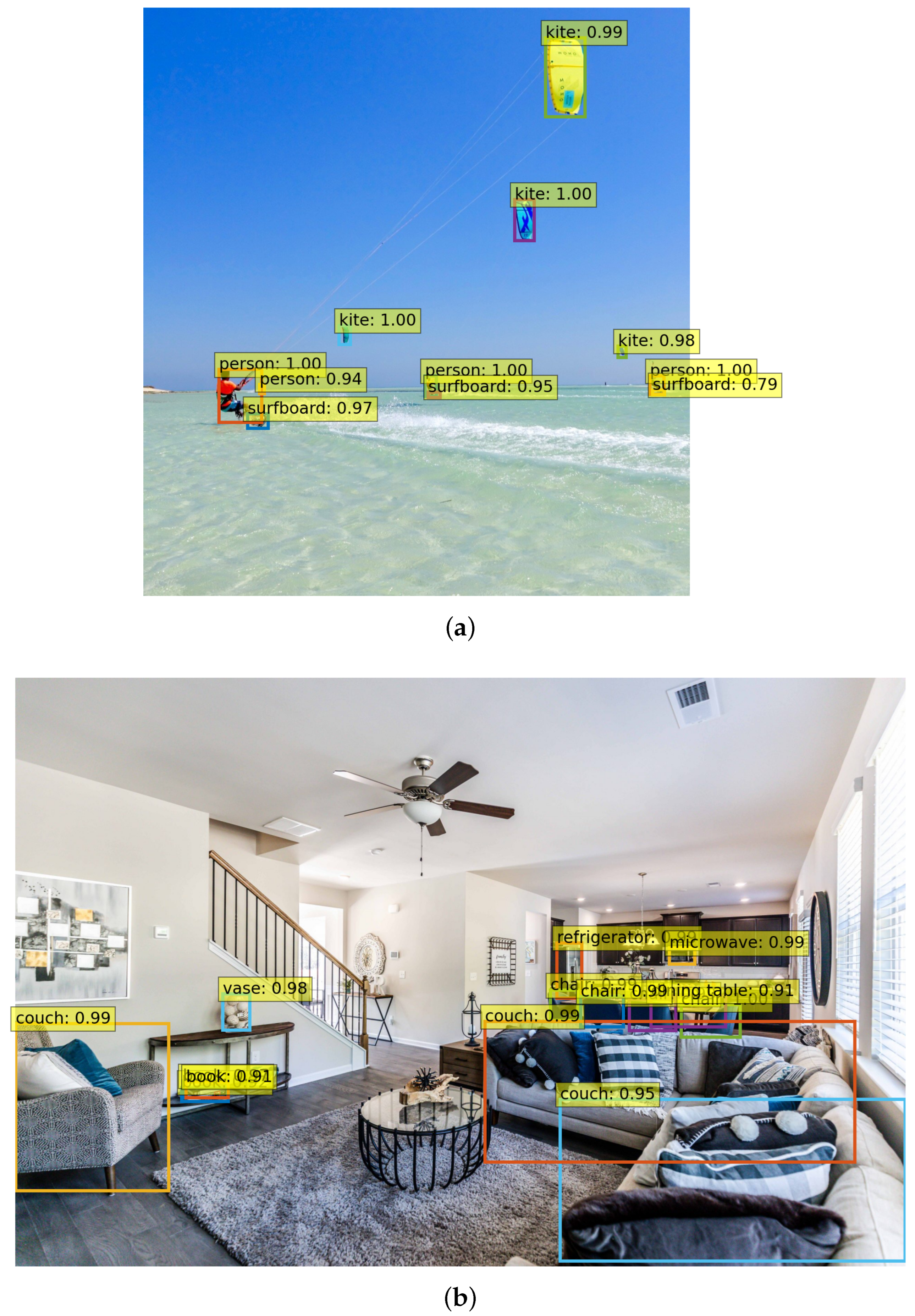
Appendix A.2. Smoke Density Detection vs. Ground Truth

Figure A2.
Examples of smoke density predictions vs. the ground truth that contributed to the low average precision (AP) of our density detectors. The first three rows are zoomed in for better illustration. (a) shows the predicted bounding boxes based on Nemo-DETR-dg. (b) Ground truth. The bounding box drawing and labeling inconsistencies significantly impact the calculated AP. The predictions on the left correctly identify the smoke region with a density that is at most one level off the ground truth. A more accurate and consistent labeling of the data could improve the calculated metrics.
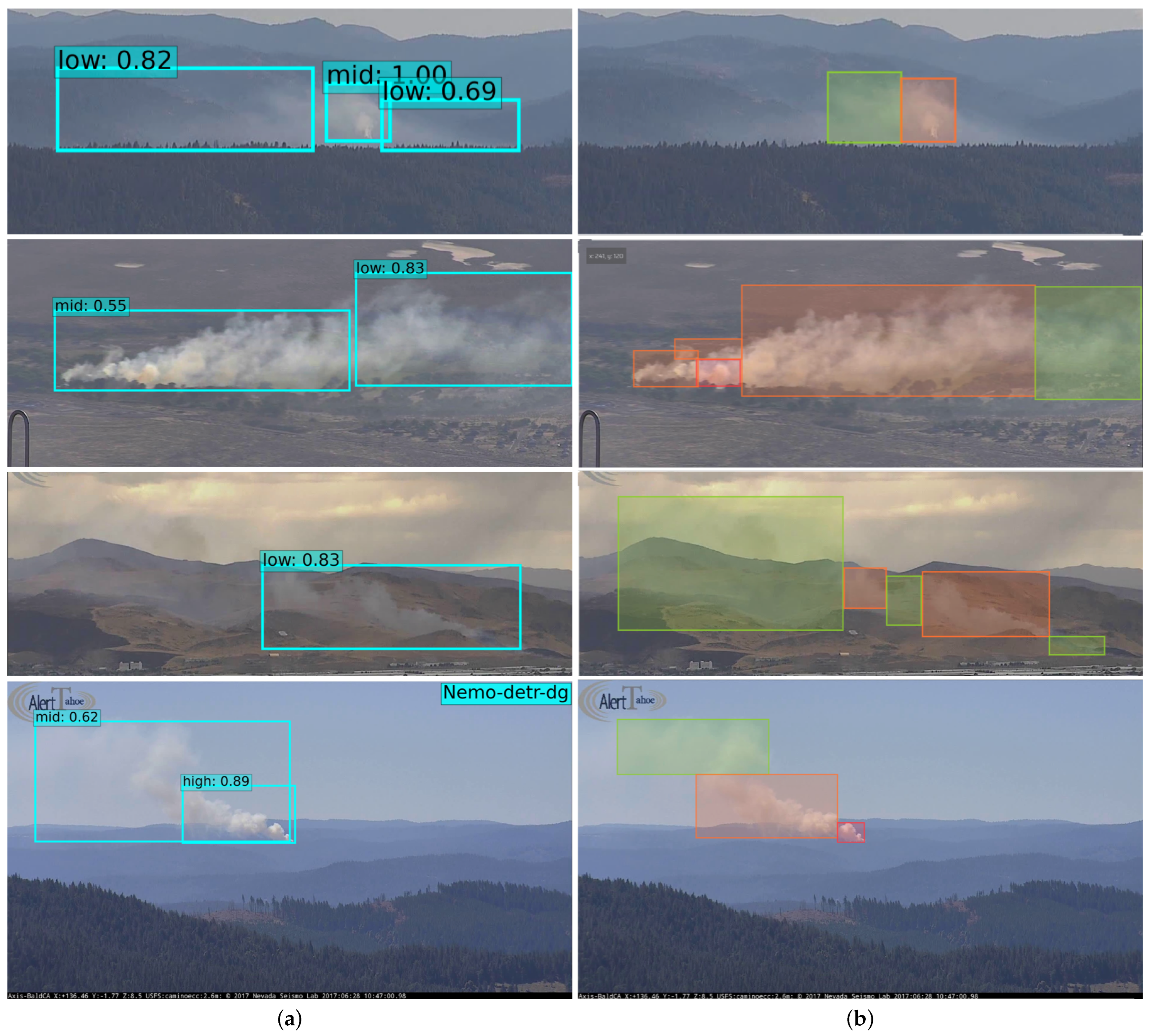
Appendix A.3. Full Time-Series Detection Results
Table A1.
The complete incipient-stage first smoke detection analysis. The first frame was used as the reference, which is 1 min after the start of the wildfire. Observations where either RNet-sc or FRCNN-sc detected smoke earlier than DETR-sc are marked in bold.
Table A1.
The complete incipient-stage first smoke detection analysis. The first frame was used as the reference, which is 1 min after the start of the wildfire. Observations where either RNet-sc or FRCNN-sc detected smoke earlier than DETR-sc are marked in bold.
| # | Video Name | Time Elapsed (min) | ||
|---|---|---|---|---|
| Nemo | ||||
| FRCNN-sc | RNet-sc | DETR-sc | ||
| 1 | 69bravo-e-mobo-c__2019-08-13 | 5 | 5 | 1 |
| 2 | 69bravo-n-mobo-c__2019-08-13 | 3 | 3 | 0 |
| 3 | bh-w-mobo-c__2019-06-10 | 9 | 10 | 4 |
| 4 | bh-w-mobo-c__2019-10-01 | N.D. | N.D. | 5 |
| 5 | bh-w-mobo-c__2019-10-03 | N.D. | N.D. | 3 |
| 6 | bl-n-mobo-c__2019-08-29 | 4 | 4 | 3 |
| 7 | bl-s-mobo-c__2019-07-16 | 8 | 8 | 3 |
| 8 | bl-s-mobo-c__2019-09-24 | 7 | 6 | 5 |
| 9 | bm-e-mobo-c__2019-10-05 | N.D. | 7 | 1 |
| 10 | hp-n-mobo-c__2019-06-29 | N.D. | 16 | 2 |
| 11 | hp-n-mobo-c__2019-07-16 | 12 | 11 | 6 |
| 12 | hp-s-mobo-c__2019-09-24 | N.D. | N.D. | 10 |
| 13 | hp-s-mobo-c__2019-10-05 | N.D. | N.D. | 4 |
| 14 | lo-s-mobo-c__2019-10-06 | 13 | 13 | 3 |
| 15 | lo-w-mobo-c__2019-09-24 | 9 | 11 | 3 |
| 16 | lo-w-mobo-c__2019-10-06 | 2 | 1 | 1 |
| 17 | lp-e-mobo-c__2019-10-06 | N.D. | N.D. | 1 |
| 18 | lp-e-mobo-c__2019-10-06 | N.D. | 21 | 29 |
| 19 | lp-n-mobo-c__2019-07-17 | 2 | 2 | 1 |
| 20 | lp-n-mobo-c__2019-07-28 | N.D. | 11 | 6 |
| 21 | lp-n-mobo-c__2019-09-24 | 4 | 5 | 1 |
| 22 | lp-n-mobo-c__2019-10-06 | 4 | 4 | 1 |
| 23 | lp-s-mobo-c__2019-08-14 | 7 | 6 | 5 |
| 24 | lp-s-mobo-c__2019-10-01 | 6 | N.D. | 2 |
| 25 | lp-s-mobo-c__2019-10-06 | 4 | 20 | 1 |
| 26 | lp-s-mobo-c__2019-10-07 | N.D. | N.D. | 3 |
| 27 | mg-n-mobo-c__2019-07-16 | 3 | 2 | 2 |
| 28 | ml-w-mobo-c__2019-09-22 | 3 | N.D. | 1 |
| 29 | ml-w-mobo-c__2019-09-24 | 4 | 4 | 3 |
| 30 | ml-w-mobo-c__2019-10-06 | 7 | 7 | 4 |
| 31 | om-e-mobo-c__2019-07-12 | 2 | 7 | 5 |
| 32 | om-e-mobo-c__2019-08-14 | 30 | 27 | 5 |
| 33 | om-e-mobo-c__2019-10-01 | 5 | 5 | 1 |
| 34 | om-n-mobo-c__2019-07-28 | N.D. | N.D. | 3 |
| 35 | om-n-mobo-c__2019-10-06 | 13 | N.D. | 2 |
| 36 | om-s-mobo-c__2019-09-30 | 3 | 2 | 1 |
| 37 | om-s-mobo-c__2019-10-01 | 10 | N.D. | 1 |
| 38 | om-s-mobo-c__2019-10-01 | 1 | 4 | 1 |
| 39 | om-s-mobo-c__2019-10-01 | 2 | N.D. | 2 |
| 40 | om-s-mobo-c__2019-10-03 | N.D. | N.D. | 2 |
| 41 | om-s-mobo-c__2019-10-06 | 18 | N.D. | 1 |
| 42 | om-s-mobo-c__2019-10-07 | N.D. | N.D. | 2 |
| 43 | om-w-mobo-c__2019-08-01 | N.D. | N.D. | N.D. |
| 44 | pi-e-mobo-c__2019-08-29 | N.D. | N.D. | N.D. |
| 45 | pi-s-mobo-c__2019-08-14 | 5 | 4 | 3 |
| 46 | pi-s-mobo-c__2019-08-26 | 31 | N.D. | 1 |
| 47 | pi-s-mobo-c__2019-10-06 | 4 | 15 | 1 |
| 48 | pi-w-mobo-c__2019-07-17 | N.D. | N.D. | 7 |
| 49 | pi-w-mobo-c__2019-09-24 | 6 | 8 | 2 |
| 50 | rm-w-mobo-c__2019-06-20 | 3 | 14 | 7 |
| 51 | rm-w-mobo-c__2019-08-26 | N.D. | N.D. | 3 |
| 52 | rm-w-mobo-c__2019-08-29 | N.D. | N.D. | 8 |
| 53 | rm-w-mobo-c__2019-10-01 | N.D. | 32 | 2 |
| 54 | rm-w-mobo-c__2019-10-03 | 2 | 3 | 1 |
| 55 | rm-w-mobo-c__2019-10-03 | 2 | 4 | 2 |
| 56 | rm-w-mobo-c__2019-10-03 | 2 | 3 | 1 |
| 57 | sdsc-e-mobo-c__2019-07-16 | N.D. | N.D. | 14 |
| 58 | sm-n-mobo-c__2019-09-24 | 8 | N.D. | 1 |
| 59 | sm-s-mobo-c__2019-10-07 | 7 | 7 | 1 |
| 60 | sm-w-mobo-c__2019-08-25 | 7 | 20 | 2 |
| 61 | smer-tcs8-mobo-c__2019-08-25 | N.D. | N.D. | 17 |
| 62 | smer-tcs8-mobo-c__2019-08-29 | 3 | 3 | 2 |
| 63 | smer-tcs9-mobo-c__2019-06-20 | 18 | N.D. | 3 |
| 64 | smer-tcs9-mobo-c__2019-10-01 | N.D. | N.D. | 4 |
| 65 | smer-tcs9-mobo-c__2019-10-01 | N.D. | 12 | 4 |
| 66 | smer-tcs9-mobo-c__2019-10-03 | N.D. | N.D. | 2 |
| 67 | smer-tcs9-mobo-c__2019-10-03 | 3 | N.D. | 1 |
| 68 | smer-tcs9-mobo-c__2019-10-03 | 4 | 3 | 1 |
| 69 | so-w-mobo-c__2019-07-16 | 0 | 2 | 0 |
| 70 | so-w-mobo-c__2019-08-27 | N.D. | N.D. | 1 |
| 71 | sp-e-mobo-c__2019-08-05 | N.D. | N.D. | 6 |
| 72 | sp-n-mobo-c__2019-07-28 | N.D. | N.D. | 8 |
| 73 | vo-n-mobo-c__2019-10-05 | 1 | 2 | 1 |
| 74 | wc-e-mobo-c__2019-09-24 | 12 | 12 | 2 |
| 75 | wc-e-mobo-c__2019-09-25 | 7 | 7 | 5 |
| 76 | wc-e-mobo-c__2019-10-05 | N.D. | N.D. | 1 |
| 77 | wc-n-mobo-c__2019-10-05 | N.D. | N.D. | 13 |
| 78 | wc-s-mobo-c__2019-09-24 | 10 | 11 | 8 |
| 79 | wc-s-mobo-c__2019-09-25 | N.D. | N.D. | 7 |
| R1: Detection rate (%) | 68.4 | 54.7 | 97.9 | |
| R2: Mean ± sd | 7.8 ± 6.9 | 10.17 ± 8.9 | 3.6 ± 4.1 | |
| R3: Mean ± sd w/imputation | 9.1 ± 7.5 | 11.4 ± 8.5 | 3.6 ± 4.1 | |
| R4: Median | 6 | 7 | 2 | |
| R5: Mean ± sd (79) | 6.8 ± 6.4 | 8.5 ± 6.9 | 3.66 ± 4.3 | |
References
- NIFC. Wildfires and Acres. Available online: https://www.nifc.gov/fire-information/statistics/wildfires (accessed on 1 February 2022).
- NOAA.gov. Wildfires–Annual 2021. Available online: https://www.ncdc.noaa.gov/sotc/fire/202113 (accessed on 1 February 2022).
- NIFC.gov. Suppression Costs. 2021. Available online: https://www.nifc.gov/fire-information/statistics/suppression-costs (accessed on 1 February 2022).
- Reid, C.E.; Brauer, M.; Johnston, F.H.; Jerrett, M.; Balmes, J.R.; Elliott, C.T. Critical Review of Health Impacts of Wildfire Smoke Exposure. Environ. Health Perspect. 2016, 124, 1334–1343. [Google Scholar] [CrossRef] [PubMed]
- Gaur, A.; Singh, A.; Kumar, A.; Kulkarni, K.S.; Lala, S.; Kapoor, K.; Srivastava, V.; Kumar, A.; Mukhopadhyay, S.C. Fire Sensing Technologies: A Review. IEEE Sens. J. 2019, 19, 3191–3202. [Google Scholar] [CrossRef]
- Barmpoutis, P.; Papaioannou, P.; Dimitropoulos, K.; Grammalidis, N. A Review on Early Forest Fire Detection Systems Using Optical Remote Sensing. Sensors 2020, 20, 6442. [Google Scholar] [CrossRef] [PubMed]
- Ba, R.; Chen, C.; Yuan, J.; Song, W.; Lo, S. SmokeNet: Satellite Smoke Scene Detection Using Convolutional Neural Network with Spatial and Channel-Wise Attention. Remote Sens. 2019, 11, 1702. [Google Scholar] [CrossRef]
- Yang, S.; Lupascu, M.; Meel, K.S. Predicting Forest Fire Using Remote Sensing Data And Machine Learning. Proc. Aaai Conf. Artif. Intell. 2021, 35, 14983–14990. [Google Scholar]
- Gholami, S.; Kodandapani, N.; Wang, J.; Lavista Ferres, J. Where there’s Smoke, there’s Fire: Wildfire Risk Predictive Modeling via Historical Climate Data. Proc. Aaai Conf. Artif. Intell. 2021, 35, 15309–15315. [Google Scholar]
- Xu, R.; Lin, H.; Lu, K.; Cao, L.; Liu, Y. A Forest Fire Detection System Based on Ensemble Learning. Forests 2021, 12, 217. [Google Scholar] [CrossRef]
- Govil, K.; Welch, M.L.; Ball, J.T.; Pennypacker, C.R. Preliminary Results from a Wildfire Detection System Using Deep Learning on Remote Camera Images. Remote Sens. 2020, 12, 166. [Google Scholar] [CrossRef]
- ALERTWildfire. ALERT Wildfire. 2022. Available online: https://www.alertwildfire.org/ (accessed on 1 February 2022).
- HPWREN. High Performance Wireless Research and Education Network. 2022. Available online: https://hpwren.ucsd.edu/ (accessed on 1 February 2022).
- The-Orange-County-Register. New Mountaintop Cameras Unveiled to Help Spot, Fight Far-Away Fires. 2018. Available online: https://www.ocregister.com/2018/05/23/new-mountaintop-cameras-unveiled-to-help-spot-fight-far-away-fires/ (accessed on 8 June 2022).
- National-Geographic. Wildfires. 2022. Available online: https://education.nationalgeographic.org/resource/wildfires (accessed on 1 February 2022).
- Guede-Fernández, F.; Martins, L.; de Almeida, R.V.; Gamboa, H.; Vieira, P. A Deep Learning Based Object Identification System for Forest Fire Detection. Fire 2021, 4, 75. [Google Scholar] [CrossRef]
- University of California San Diego. The HPWREN Fire Ignition Images Library for Neural Network Training. 2022. Available online: http://hpwren.ucsd.edu/HPWREN-FIgLib/ (accessed on 1 February 2022).
- Borges, P.V.K.; Izquierdo, E. A Probabilistic Approach for Vision-Based Fire Detection in Videos. IEEE Trans. Circuits Syst. Video Technol. 2010, 20, 721–731. [Google Scholar] [CrossRef]
- Zhang, Z.; Shen, T.; Zou, J. An Improved Probabilistic Approach for Fire Detection in Videos. Fire Technol. 2014, 50, 745–752. [Google Scholar] [CrossRef]
- Toreyin, B.U.; DedeogElu, Y.; Gudukbay, U.; Aetin, A.E. Computer vision based method for real-time fire and flame detection. Pattern Recognit. Lett. 2006, 27, 49–58. [Google Scholar] [CrossRef]
- Zhang, Q.; Xu, J.; Xu, L.; Guo, H. Deep Convolutional Neural Networks for Forest Fire Detection. In Proceedings of the 2016 International Forum on Management, Education and Information Technology Application, Guangzhou, China, 30–31 January 2016; pp. 568–575. [Google Scholar] [CrossRef]
- Wu, S.; Zhang, L. Using Popular Object Detection Methods for Real Time Forest Fire Detection. In Proceedings of the 2018 11th International Symposium on Computational Intelligence and Design (ISCID), Hangzhou, China, 8–9 December 2018; Volume 1, pp. 280–284. [Google Scholar] [CrossRef]
- Kim, B.; Lee, J. A Video-Based Fire Detection Using Deep Learning Models. Appl. Sci. 2019, 9, 2862. [Google Scholar] [CrossRef]
- Muhammad, K.; Ahmad, J.; Mehmood, I.; Rho, S.; Baik, S.W. Convolutional Neural Networks Based Fire Detection in Surveillance Videos. IEEE Access 2018, 6, 18174–18183. [Google Scholar] [CrossRef]
- Muhammad, K.; Ahmad, J.; Baik, S.W. Early fire detection using convolutional neural networks during surveillance for effective disaster management. Neurocomputing 2018, 288, 30–42. [Google Scholar] [CrossRef]
- Muhammad, K.; Ahmad, J.; Lv, Z.; Bellavista, P.; Yang, P.; Baik, S.W. Efficient Deep CNN-Based Fire Detection and Localization in Video Surveillance Applications. IEEE Trans. Syst. Man Cybern. Syst. 2019, 49, 1419–1434. [Google Scholar] [CrossRef]
- Muhammad, K.; Khan, S.; Elhoseny, M.; Hassan Ahmed, S.; Wook Baik, S. Efficient Fire Detection for Uncertain Surveillance Environment. IEEE Trans. Ind. Inform. 2019, 15, 3113–3122. [Google Scholar] [CrossRef]
- Jeon, M.; Choi, H.S.; Lee, J.; Kang, M. Multi-Scale Prediction For Fire Detection Using Convolutional Neural Network. Fire Technol. 2021, 57, 2533–2551. [Google Scholar] [CrossRef]
- Chaoxia, C.; Shang, W.; Zhang, F. Information-Guided Flame Detection Based on Faster R-CNN. IEEE Access 2020, 8, 58923–58932. [Google Scholar] [CrossRef]
- Park, M.; Tran, D.Q.; Jung, D.; Park, S. Wildfire-Detection Method Using DenseNet and CycleGAN Data Augmentation-Based Remote Camera Imagery. Remote Sens. 2020, 12, 3715. [Google Scholar] [CrossRef]
- Li, P.; Zhao, W. Image fire detection algorithms based on convolutional neural networks. Case Stud. Therm. Eng. 2020, 19, 100625. [Google Scholar] [CrossRef]
- Ajith, M.; Martínez-Ramón, M. Unsupervised Segmentation of Fire and Smoke From Infra-Red Videos. IEEE Access 2019, 7, 182381–182394. [Google Scholar] [CrossRef]
- NAMOZOV, A.; CHO, Y.I. An Efficient Deep Learning Algorithm for Fire and Smoke Detection with Limited Data. Adv. Electr. Comput. Eng. 2018, 18, 121–128. [Google Scholar] [CrossRef]
- Saponara, S.; Elhanashi, A.; Gagliardi, A. Real-time video fire/smoke detection based on CNN in antifire surveillance systems. J. Real Time Image Process. 2021, 18, 889–900. [Google Scholar] [CrossRef]
- Donida Labati, R.; Genovese, A.; Piuri, V.; Scotti, F. Wildfire Smoke Detection Using Computational Intelligence Techniques Enhanced With Synthetic Smoke Plume Generation. IEEE Trans. Syst. Man, Cybern. Syst. 2013, 43, 1003–1012. [Google Scholar] [CrossRef]
- IQ FireWatch Technology. Available online: https://www.iq-firewatch.com/technology (accessed on 10 February 2022).
- ForestWatch. Available online: http://evsusa.biz/productsservices/forestwatch/ (accessed on 10 February 2022).
- Pan, H.; Badawi, D.; Cetin, A.E. Computationally Efficient Wildfire Detection Method Using a Deep Convolutional Network Pruned via Fourier Analysis. Sensors 2020, 20, 2891. [Google Scholar] [CrossRef]
- Lin, T.Y.; Dollar, P.; Girshick, R.; He, K.; Hariharan, B.; Belongie, S. Feature Pyramid Networks for Object Detection. In Proceedings of the IEEE Conference on Computer Vision and Pattern Recognition (CVPR), Honolulu, HI, USA, 21–26 July 2017. [Google Scholar]
- Tan, M.; Pang, R.; Le, Q.V. EfficientDet: Scalable and Efficient Object Detection. In Proceedings of the IEEE/CVF Conference on Computer Vision and Pattern Recognition (CVPR), Seattle, WA, USA, 13–19 June 2020. [Google Scholar]
- Lin, T.Y.; Goyal, P.; Girshick, R.; He, K.; Dollar, P. Focal Loss for Dense Object Detection. In Proceedings of the IEEE International Conference on Computer Vision (ICCV), Venice, Italy, 22–29 October 2017. [Google Scholar]
- Redmon, J.; Farhadi, A. Yolov3: An incremental improvement. arXiv 2018, arXiv:1804.02767. [Google Scholar]
- Jocher, G. ultralytics/yolov5: V3.1—Bug Fixes and Performance Improvements. 2020. Available online: https://github.com/ultralytics/yolov5 (accessed on 1 February 2022).
- Devlin, J.; Chang, M.W.; Lee, K.; Toutanova, K. BERT: Pre-training of Deep Bidirectional Transformers for Language Understanding. arXiv 2018, arXiv:1810.04805. [Google Scholar] [CrossRef]
- Yang, Z.; Xu, C.; Li, L. Landslide Detection Based on ResU-Net with Transformer and CBAM Embedded: Two Examples with Geologically Different Environments. Remote Sens. 2022, 14, 2885. [Google Scholar] [CrossRef]
- Ghali, R.; Akhloufi, M.A.; Jmal, M.; Souidene Mseddi, W.; Attia, R. Wildfire Segmentation Using Deep Vision Transformers. Remote Sens. 2021, 13, 3527. [Google Scholar] [CrossRef]
- Carion, N.; Massa, F.; Synnaeve, G.; Usunier, N.; Kirillov, A.; Zagoruyko, S. End-to-End Object Detection with Transformers. In Proceedings of the Computer Vision—ECCV 2020; Vedaldi, A., Bischof, H., Brox, T., Frahm, J.M., Eds.; Springer International Publishing: Cham, Switzerland, 2020; pp. 213–229. [Google Scholar]
- Yazdi, A. Nemo: Nevada Smoke Detection Benchmark. 2022. Available online: https://github.com/SayBender/Nemo (accessed on 1 August 2022).
- Jiao, Z.; Zhang, Y.; Mu, L.; Xin, J.; Jiao, S.; Liu, H.; Liu, D. A YOLOv3-based Learning Strategy for Real-time UAV-based Forest Fire Detection. In Proceedings of the 2020 Chinese Control And Decision Conference (CCDC), Hefei, China, 22–24 August 2020; pp. 4963–4967. [Google Scholar] [CrossRef]
- Jiao, Z.; Zhang, Y.; Xin, J.; Mu, L.; Yi, Y.; Liu, H.; Liu, D. A Deep Learning Based Forest Fire Detection Approach Using UAV and YOLOv3. In Proceedings of the 2019 1st International Conference on Industrial Artificial Intelligence (IAI), Shenyang, China, 22–26 July 2019; pp. 1–5. [Google Scholar] [CrossRef]
- Barmpoutis, P.; Dimitropoulos, K.; Kaza, K.; Grammalidis, N. Fire detection from images using faster R-CNN and multidimensional texture analysis. In Proceedings of the ICASSP 2019-2019 IEEE International Conference on Acoustics, Speech and Signal Processing (ICASSP), Brighton, UK, 12–17 May 2019; pp. 8301–8305. [Google Scholar]
- Yin, Z.; Wan, B.; Yuan, F.; Xia, X.; Shi, J. A Deep Normalization and Convolutional Neural Network for Image Smoke Detection. IEEE Access 2017, 5, 18429–18438. [Google Scholar] [CrossRef]
- Healey, G.; Slater, D.; Lin, T.; Drda, B.; Goedeke, A. A system for real-time fire detection. In Proceedings of the IEEE Conference on Computer Vision and Pattern Recognition, New York, NY, USA, 15–17 June 1993; pp. 605–606. [Google Scholar] [CrossRef]
- CHEN, T.H.; WU, P.H.; CHIOU, Y.C. An early fire-detection method based on image processing. In Proceedings of the 2004 International Conference on Image Processing (ICIP ’04), Singapore, 24–27 October 2004; IEEE: Piscataway, NJ, USA, 2004; Volume 3, pp. 1707–1710. [Google Scholar]
- Horng, W.B.; Peng, J.W.; Chen, C.Y. A new image-based real-time flame detection method using color analysis. In Proceedings of the 2005 IEEE Networking, Sensing and Control, Tucson, AZ, USA, 19–22 March 2005; pp. 100–105. [Google Scholar] [CrossRef]
- Chino, D.Y.T.; Avalhais, L.P.S.; Rodrigues, J.F.; Traina, A.J.M. BoWFire: Detection of Fire in Still Images by Integrating Pixel Color and Texture Analysis. In Proceedings of the 2015 28th SIBGRAPI Conference on Graphics, Patterns and Images, Salvador, Brazil, 26–29 August 2015; pp. 95–102. [Google Scholar] [CrossRef]
- Ko, B.C.; Cheong, K.H.; Nam, J.Y. Fire detection based on vision sensor and support vector machines. Fire Saf. J. 2009, 44, 322–329. [Google Scholar] [CrossRef]
- Foggia, P.; Saggese, A.; Vento, M. Real-Time Fire Detection for Video-Surveillance Applications Using a Combination of Experts Based on Color, Shape, and Motion. IEEE Trans. Circuits Syst. Video Technol. 2015, 25, 1545–1556. [Google Scholar] [CrossRef]
- Prema, C.E.; Vinsley, S.S.; Suresh, S. Efficient Flame Detection Based on Static and Dynamic Texture Analysis in Forest Fire Detection. Fire Technol. 2017, 54, 255–288. [Google Scholar] [CrossRef]
- Gholamnia, K.; Gudiyangada Nachappa, T.; Ghorbanzadeh, O.; Blaschke, T. Comparisons of Diverse Machine Learning Approaches for Wildfire Susceptibility Mapping. Symmetry 2020, 12, 604. [Google Scholar] [CrossRef]
- Abdollahi, A.; Pradhan, B.; Shukla, N.; Chakraborty, S.; Alamri, A. Deep Learning Approaches Applied to Remote Sensing Datasets for Road Extraction: A State-Of-The-Art Review. Remote Sens. 2020, 12, 1444. [Google Scholar] [CrossRef]
- Kamilaris, A.; Prenafeta-Boldú, F.X. Deep learning in agriculture: A survey. Comput. Electron. Agric. 2018, 147, 70–90. [Google Scholar] [CrossRef]
- Litjens, G.; Kooi, T.; Bejnordi, B.E.; Setio, A.A.A.; Ciompi, F.; Ghafoorian, M.; van der Laak, J.A.; van Ginneken, B.; Sánchez, C.I. A survey on deep learning in medical image analysis. Med. Image Anal. 2017, 42, 60–88. [Google Scholar] [CrossRef]
- Ghorbanzadeh, O.; Crivellari, A.; Ghamisi, P.; Shahabi, H.; Blaschke, T. A comprehensive transferability evaluation of U-Net and ResU-Net for landslide detection from Sentinel-2 data (case study areas from Taiwan, China, and Japan). Sci. Rep. 2021, 11, 14629. [Google Scholar] [CrossRef]
- Ghorbanzadeh, O.; Xu, Y.; Ghamisi, P.; Kopp, M.; Kreil, D. Landslide4Sense: Reference Benchmark Data and Deep Learning Models for Landslide Detection. arXiv 2022, arXiv:2206.00515. [Google Scholar] [CrossRef]
- Minaee, S.; Boykov, Y.Y.; Porikli, F.; Plaza, A.J.; Kehtarnavaz, N.; Terzopoulos, D. Image Segmentation Using Deep Learning: A Survey. IEEE Trans. Pattern Anal. Mach. Intell. 2021, 44, 3523–3542. [Google Scholar] [CrossRef] [PubMed]
- Zhao, Z.Q.; Zheng, P.; Xu, S.T.; Wu, X. Object Detection With Deep Learning: A Review. IEEE Trans. Neural Netw. Learn. Syst. 2019, 30, 3212–3232. [Google Scholar] [CrossRef] [PubMed]
- Redmon, J.; Divvala, S.; Girshick, R.; Farhadi, A. You Only Look Once: Unified, Real-Time Object Detection. In Proceedings of the IEEE Conference on Computer Vision and Pattern Recognition (CVPR), Las Vegas, NV, USA, 27–30 June 2016. [Google Scholar]
- Redmon, J.; Farhadi, A. YOLO9000: Better, Faster, Stronger. In Proceedings of the IEEE Conference on Computer Vision and Pattern Recognition (CVPR), Honolulu, HI, USA, 21–26 July 2017. [Google Scholar]
- Liu, W.; Anguelov, D.; Erhan, D.; Szegedy, C.; Reed, S.; Fu, C.Y.; Berg, A.C. Ssd: Single shot multibox detector. In Proceedings of the European Conference on Computer Vision, Amsterdam, The Netherlands, 11–14 October 2016; pp. 21–37. [Google Scholar]
- Zhu, X.; Su, W.; Lu, L.; Li, B.; Wang, X.; Dai, J. Deformable DETR: Deformable Transformers for End-to-End Object Detection. arXiv 2020, arXiv:2010.04159. [Google Scholar]
- Girshick, R.; Donahue, J.; Darrell, T.; Malik, J. Rich Feature Hierarchies for Accurate Object Detection and Semantic Segmentation. In Proceedings of the IEEE Conference on Computer Vision and Pattern Recognition (CVPR), Columbus, OH, USA, 23–28 June 2014. [Google Scholar]
- Ren, S.; He, K.; Girshick, R.; Sun, J. Faster R-CNN: Towards Real-Time Object Detection with Region Proposal Networks. In Proceedings of the Advances in Neural Information Processing Systems; Cortes, C., Lawrence, N., Lee, D., Sugiyama, M., Garnett, R., Eds.; Curran Associates, Inc.: Red Hook, NY, USA, 2015; Volume 28. [Google Scholar]
- He, K.; Gkioxari, G.; Dollar, P.; Girshick, R. Mask R-CNN. In Proceedings of the IEEE International Conference on Computer Vision (ICCV), Venice, Italy, 22–29 October 2017. [Google Scholar]
- Jiao, L.; Zhang, F.; Liu, F.; Yang, S.; Li, L.; Feng, Z.; Qu, R. A Survey of Deep Learning-Based Object Detection. IEEE Access 2019, 7, 128837–128868. [Google Scholar] [CrossRef]
- Uijlings, J.R.; Van De Sande, K.E.; Gevers, T.; Smeulders, A.W. Selective search for object recognition. Int. J. Comput. Vis. 2013, 104, 154–171. [Google Scholar] [CrossRef]
- Jain, P.; Coogan, S.C.; Subramanian, S.G.; Crowley, M.; Taylor, S.; Flannigan, M.D. A review of machine learning applications in wildfire science and management. Environ. Rev. 2020, 28, 478–505. [Google Scholar] [CrossRef]
- Szegedy, C.; Liu, W.; Jia, Y.; Sermanet, P.; Reed, S.; Anguelov, D.; Erhan, D.; Vanhoucke, V.; Rabinovich, A. Going Deeper With Convolutions. In Proceedings of the IEEE Conference on Computer Vision and Pattern Recognition (CVPR), Boston, MA, USA, 7–12 June 2015. [Google Scholar]
- Krizhevsky, A.; Sutskever, I.; Hinton, G.E. ImageNet Classification with Deep Convolutional Neural Networks. In Proceedings of the Advances in Neural Information Processing Systems; Pereira, F., Burges, C.J.C., Bottou, L., Weinberger, K.Q., Eds.; Curran Associates, Inc.: Red Hook, NY, USA, 2012; Volume 25. [Google Scholar]
- Sandler, M.; Howard, A.; Zhu, M.; Zhmoginov, A.; Chen, L.C. MobileNetV2: Inverted Residuals and Linear Bottlenecks. In Proceedings of the IEEE Conference on Computer Vision and Pattern Recognition (CVPR), Salt Lake City, UT, USA, 18–23 June 2018. [Google Scholar]
- Zhang, Q.X.; Lin, G.H.; Zhang, Y.M.; Xu, G.; Wang, J.J. Wildland Forest Fire Smoke Detection Based on Faster R-CNN using Synthetic Smoke Images. Procedia Eng. 2018, 211, 441–446. [Google Scholar] [CrossRef]
- Szegedy, C.; Vanhoucke, V.; Ioffe, S.; Shlens, J.; Wojna, Z. Rethinking the Inception Architecture for Computer Vision. In Proceedings of the IEEE Conference on Computer Vision and Pattern Recognition (CVPR), Las Vegas, NV, USA, 27–30 June 2016. [Google Scholar]
- Huang, G.; Liu, Z.; van der Maaten, L.; Weinberger, K.Q. Densely Connected Convolutional Networks. In Proceedings of the IEEE Conference on Computer Vision and Pattern Recognition (CVPR), Honolulu, HI, USA, 21–26 July 2017. [Google Scholar]
- Goodfellow, I.; Pouget-Abadie, J.; Mirza, M.; Xu, B.; Warde-Farley, D.; Ozair, S.; Courville, A.; Bengio, Y. Generative Adversarial Nets. In Proceedings of the Advances in Neural Information Processing Systems; Ghahramani, Z., Welling, M., Cortes, C., Lawrence, N., Weinberger, K.Q., Eds.; Curran Associates, Inc.: Red Hook, NY, USA, 2014; Volume 27. [Google Scholar]
- Zhu, J.Y.; Park, T.; Isola, P.; Efros, A.A. Unpaired Image-To-Image Translation Using Cycle-Consistent Adversarial Networks. In Proceedings of the IEEE International Conference on Computer Vision (ICCV), Venice, Italy, 22–29 October 2017. [Google Scholar]
- Dai, J.; Li, Y.; He, K.; Sun, J. R-FCN: Object Detection via Region-based Fully Convolutional Networks. In Proceedings of the Advances in Neural Information Processing Systems; Lee, D., Sugiyama, M., Luxburg, U., Guyon, I., Garnett, R., Eds.; Curran Associates, Inc.: Red Hook, NY, USA, 2016; Volume 29. [Google Scholar]
- Tan, M.; Le, Q. EfficientNet: Rethinking Model Scaling for Convolutional Neural Networks. In Proceedings of the 36th International Conference on Machine Learning, Long Beach, CA, USA, 9–15 June 2019; Volume 97, pp. 6105–6114. [Google Scholar]
- Dosovitskiy, A.; Beyer, L.; Kolesnikov, A.; Weissenborn, D.; Zhai, X.; Unterthiner, T.; Dehghani, M.; Minderer, M.; Heigold, G.; Gelly, S.; et al. An Image is Worth 16x16 Words: Transformers for Image Recognition at Scale. arXiv 2021, arXiv:2010.11929. [Google Scholar] [CrossRef]
- Khan, S.; Naseer, M.; Hayat, M.; Zamir, S.W.; Khan, F.S.; Shah, M. Transformers in Vision: A Survey. ACM Comput. Surv. 2021. [Google Scholar] [CrossRef]
- Dai, Z.; Cai, B.; Lin, Y.; Chen, J. UP-DETR: Unsupervised Pre-Training for Object Detection With Transformers. In Proceedings of the IEEE/CVF Conference on Computer Vision and Pattern Recognition (CVPR), Virtual, 19–25 June 2021; pp. 1601–1610. [Google Scholar]
- Dai, X.; Chen, Y.; Yang, J.; Zhang, P.; Yuan, L.; Zhang, L. Dynamic DETR: End-to-End Object Detection With Dynamic Attention. In Proceedings of the IEEE/CVF International Conference on Computer Vision (ICCV), Montreal, QC, Canada, 10–17 October 2021; pp. 2988–2997. [Google Scholar]
- Tavakkoli Piralilou, S.; Einali, G.; Ghorbanzadeh, O.; Nachappa, T.G.; Gholamnia, K.; Blaschke, T.; Ghamisi, P. A Google Earth Engine Approach for Wildfire Susceptibility Prediction Fusion with Remote Sensing Data of Different Spatial Resolutions. Remote Sens. 2022, 14, 672. [Google Scholar] [CrossRef]
- Abdi, O.; Kamkar, B.; Shirvani, Z.; da Silva, J.A.T.; Buchroithner, M.F. Spatial-statistical analysis of factors determining forest fires: A case study from Golestan, Northeast Iran. Geomat. Nat. Hazards Risk 2018, 9, 267–280. [Google Scholar] [CrossRef]
- NSL. Nevada Seismological Lab. 2022. Available online: http://www.seismo.unr.edu/ (accessed on 1 February 2022).
- Skalski, P. Make Sense. 2019. Available online: https://github.com/SkalskiP/make-sense/ (accessed on 1 February 2022).
- Vaswani, A.; Shazeer, N.; Parmar, N.; Uszkoreit, J.; Jones, L.; Gomez, A.N.; Kaiser, L.; Polosukhin, I. Attention is All You Need. In Proceedings of the 31st International Conference on Neural Information Processing Systems; Curran Associates Inc.: Red Hook, NY, USA, 2017; pp. 6000–6010. [Google Scholar]
- Rezatofighi, H.; Tsoi, N.; Gwak, J.; Sadeghian, A.; Reid, I.; Savarese, S. Generalized Intersection Over Union: A Metric and a Loss for Bounding Box Regression. In Proceedings of the IEEE/CVF Conference on Computer Vision and Pattern Recognition (CVPR), Long Beach, CA, USA, 16–20 June 2019. [Google Scholar]
- COCO-Common Objects in Context. 2022. Available online: https://cocodataset.org/#explore (accessed on 1 February 2022).
- An Unprecedented Colorado Wildfire is Burning Despite the Presence of Snow on the Ground. Available online: https://www.salon.com/2022/03/31/an-unprecedented-colorado-wildfire-is-burning-despite-the-presence-of-snow-on-the-ground/ (accessed on 16 June 2022).
- Massa, F. PyTorch Vision Releases. 2022. Available online: https://github.com/pytorch/vision/releases (accessed on 1 February 2022).
- COCO-API. 2022. Available online: https://github.com/cocodataset/cocoapi/blob/master/PythonAPI/pycocotools/cocoeval.py (accessed on 1 February 2022).
- Govil, K. Firecam Datasets. 2022. Available online: https://github.com/open-climate-tech/firecam/tree/master/datasets (accessed on 1 February 2022).
- NPS.GOV. The United States National Parks Services. Wildfire Causes and Evaluations. 2022. Available online: https://www.nps.gov/articles/wildfire-causes-and-evaluation.htm (accessed on 1 February 2022).
- Facebook. DETR Hands-On Collab. 2022. Available online: https://colab.research.google.com/github/facebookresearch/detr/blob/colab/notebooks/detr_attention.ipynb (accessed on 1 February 2022).

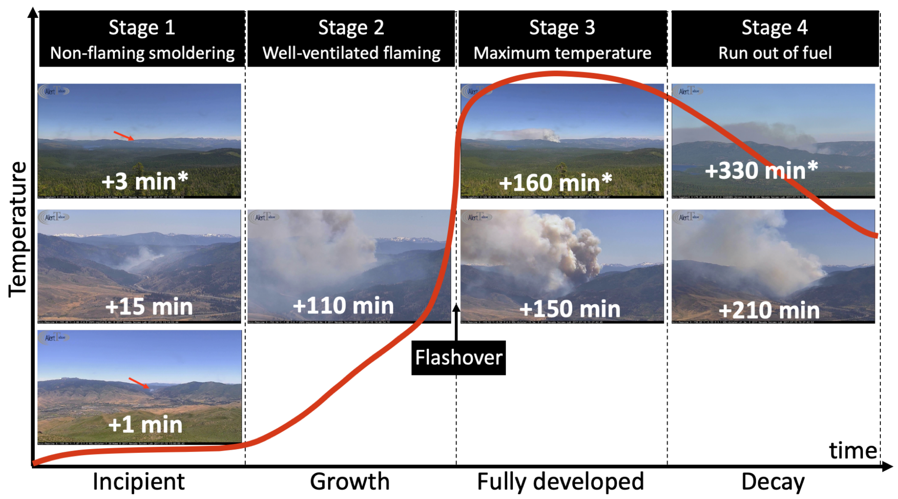
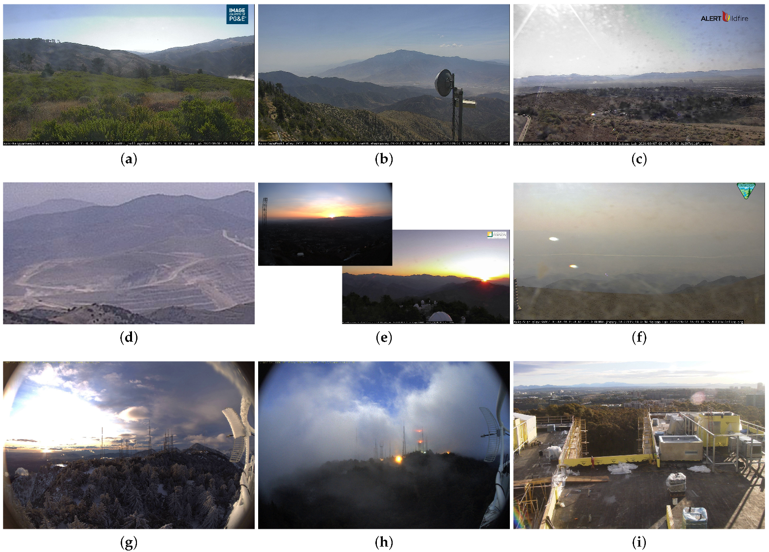

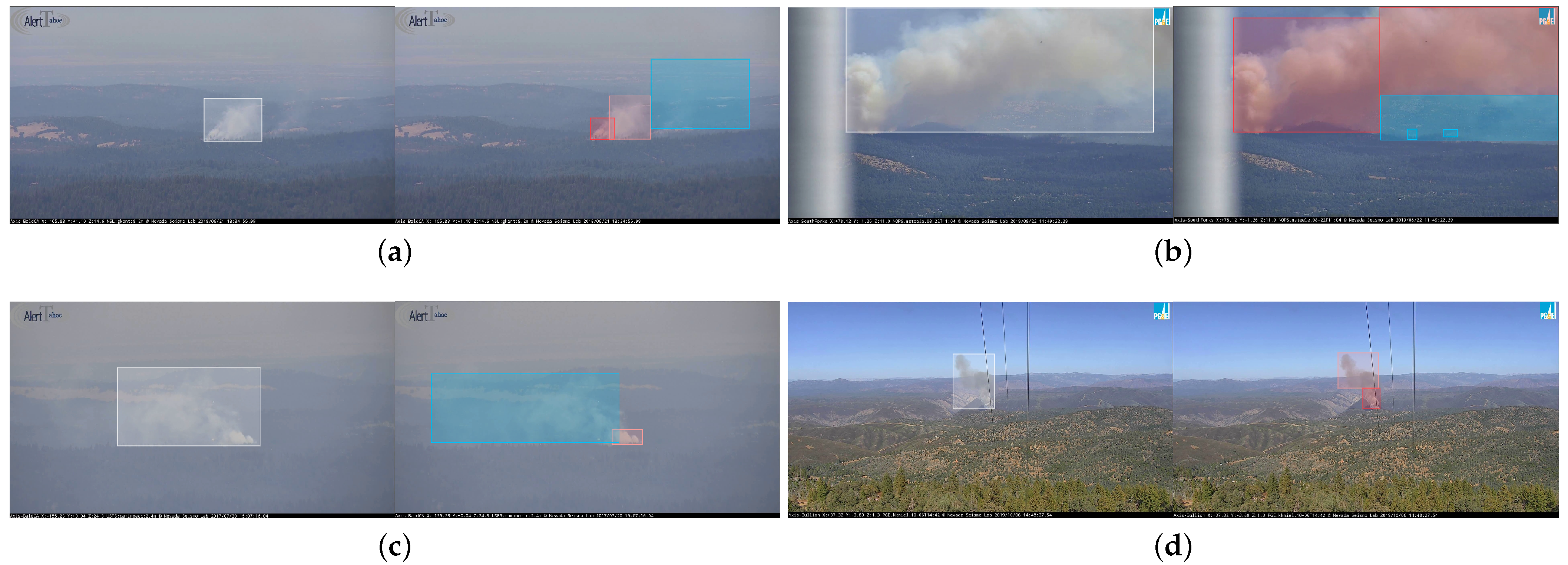
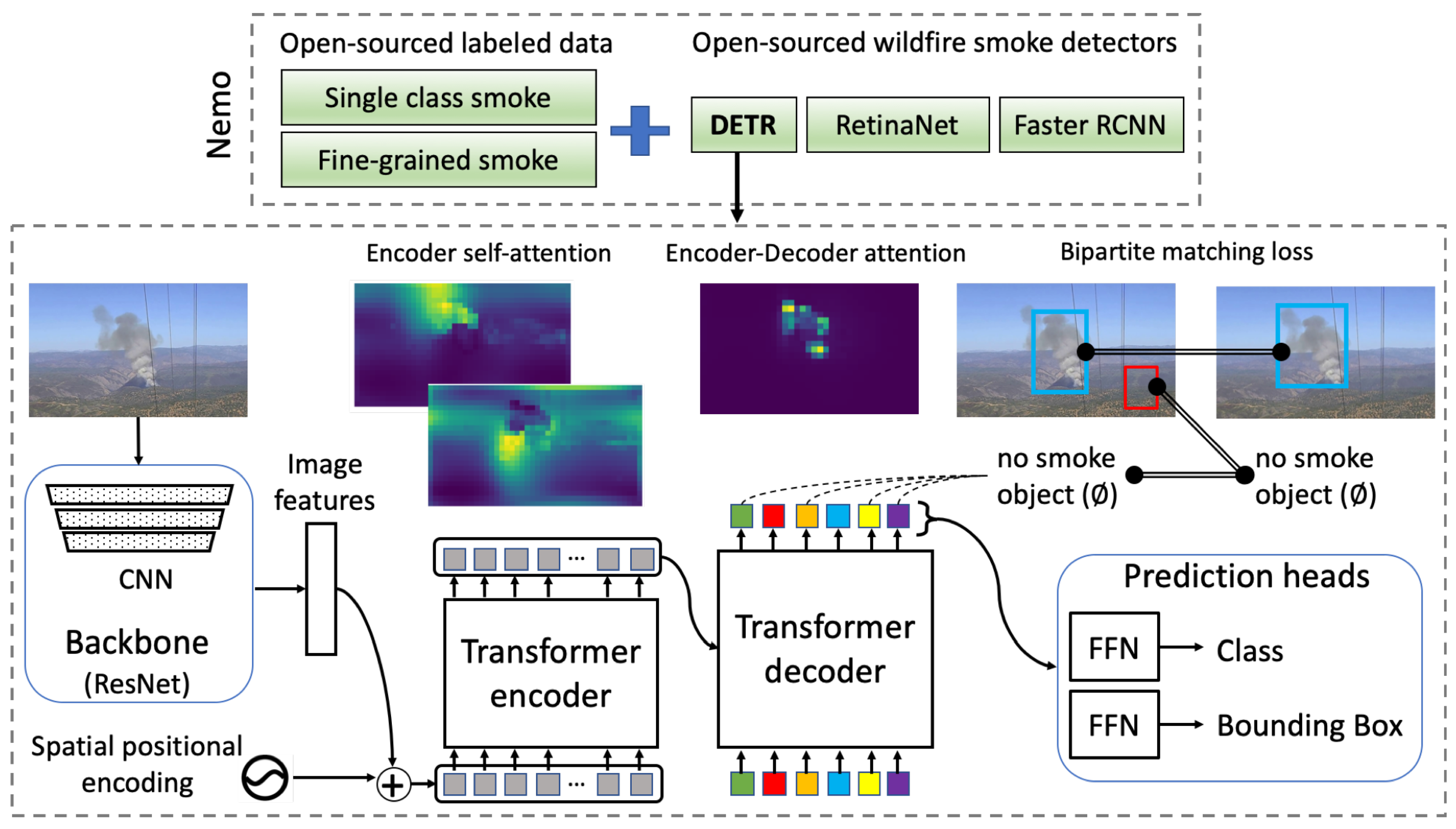


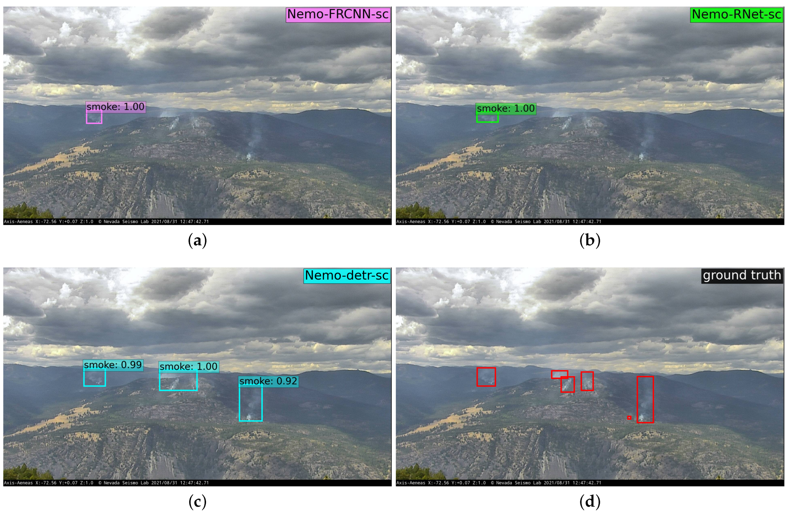
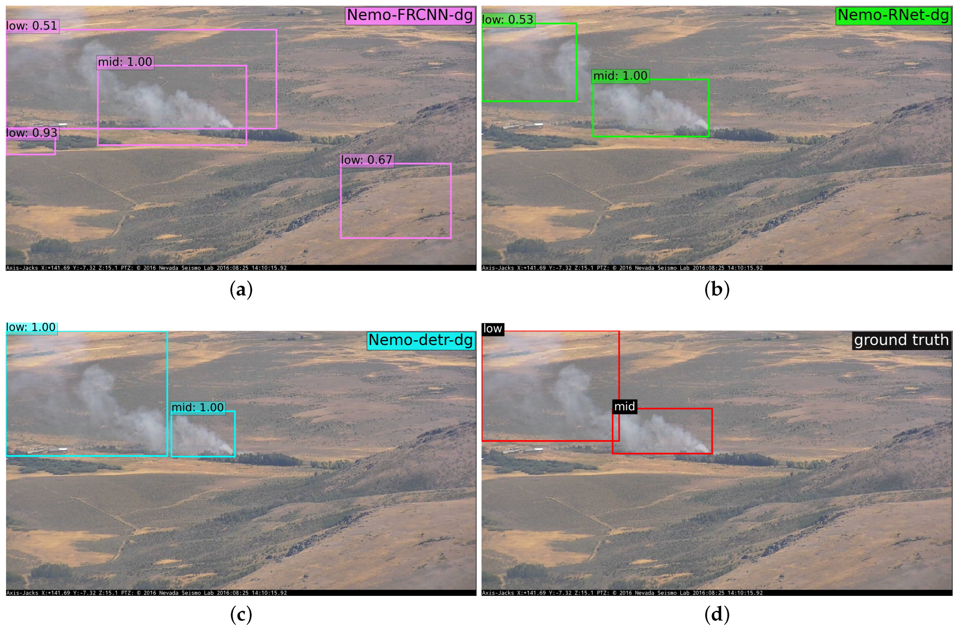
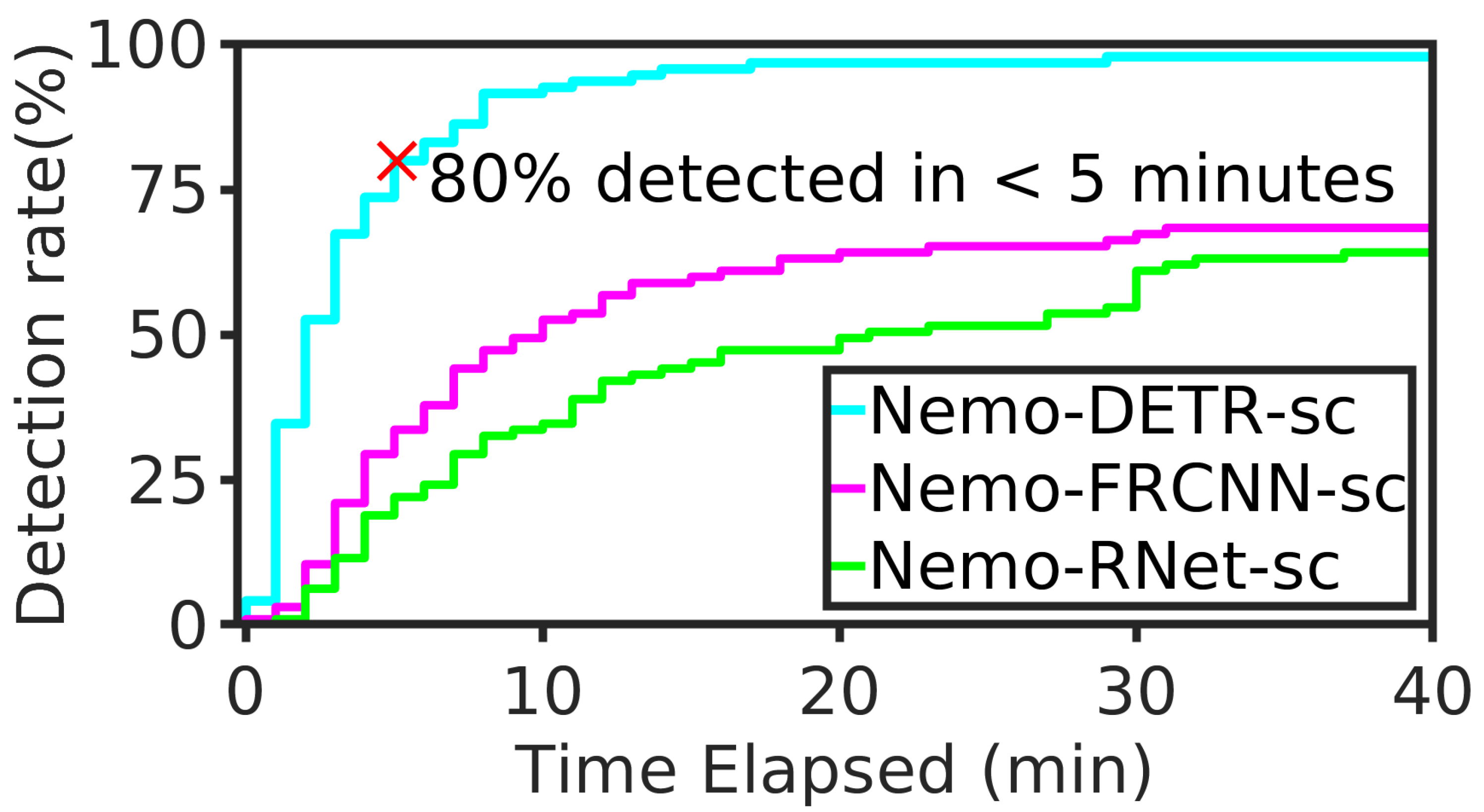
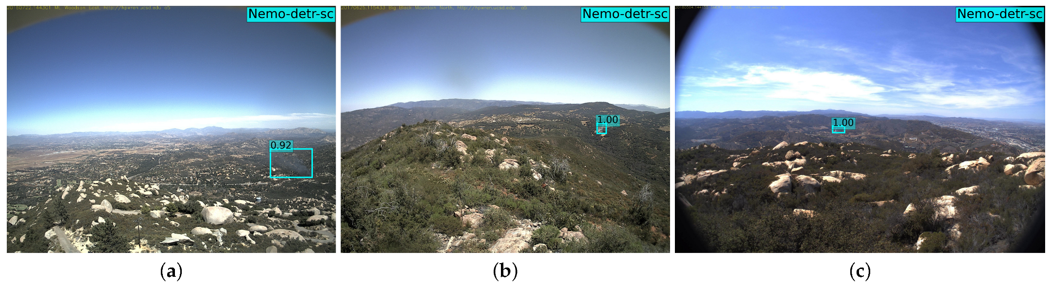

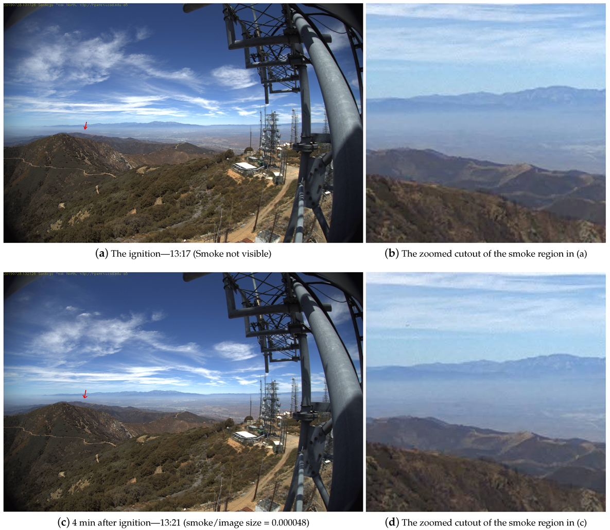
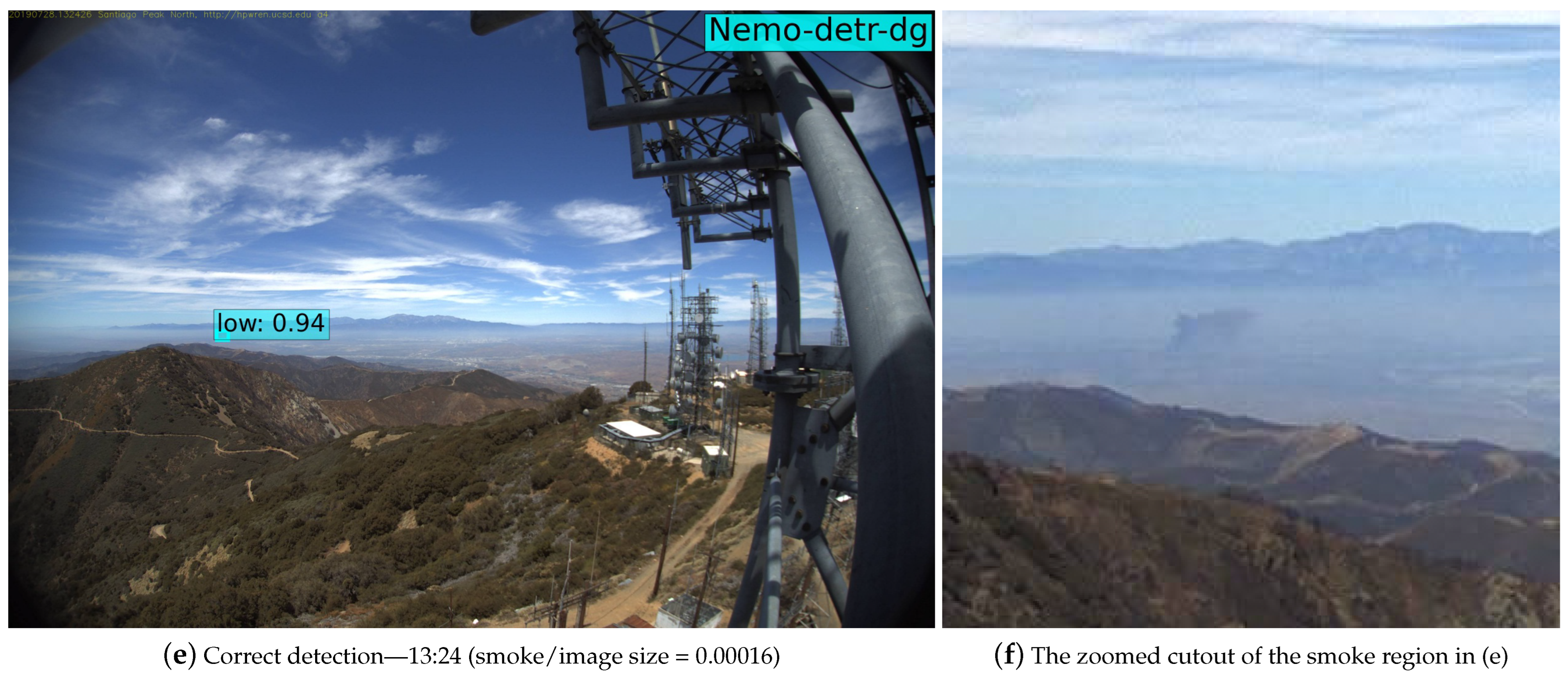
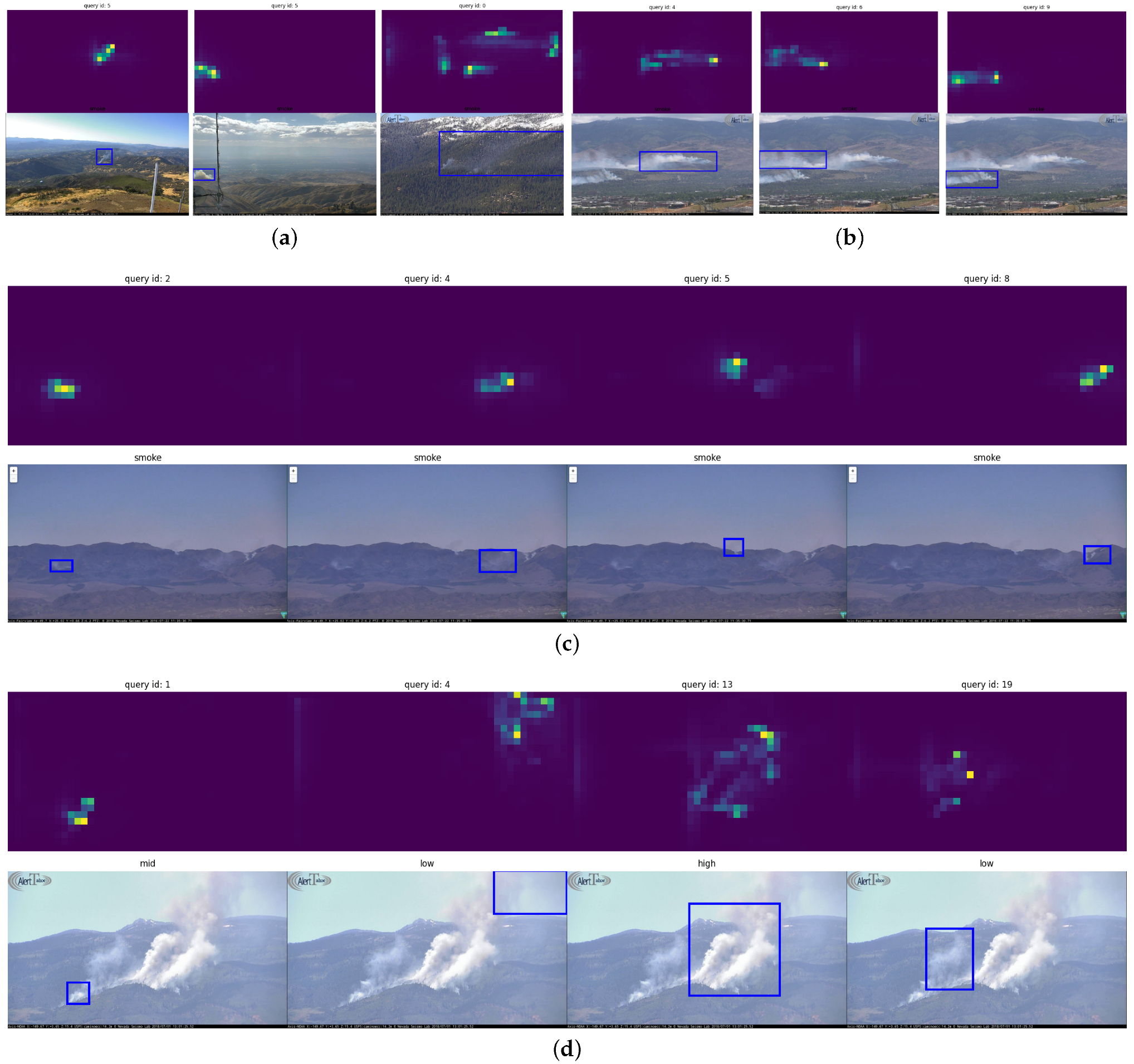
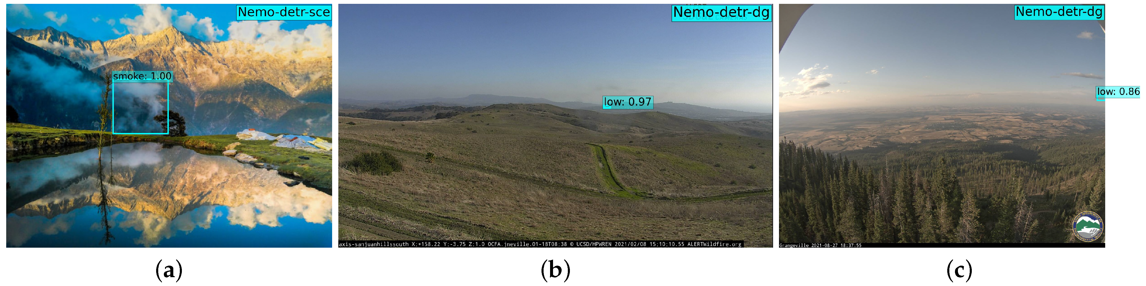
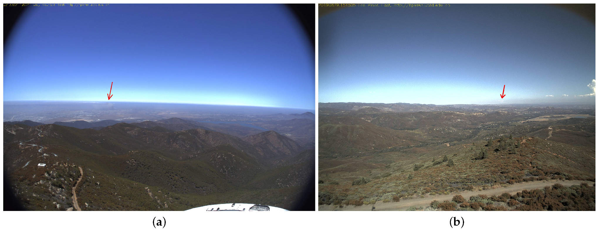
Publisher’s Note: MDPI stays neutral with regard to jurisdictional claims in published maps and institutional affiliations. |
© 2022 by the authors. Licensee MDPI, Basel, Switzerland. This article is an open access article distributed under the terms and conditions of the Creative Commons Attribution (CC BY) license (https://creativecommons.org/licenses/by/4.0/).