3D Convolutional Neural Network for Low-Light Image Sequence Enhancement in SLAM

Abstract

Typical visual simultaneous localization and mapping (SLAM) systems rely on front-end odometry for feature extraction and matching to establish the relations between adjacent images. In a low-light environment, the image obtained by a camera is dim and shows scarce information, hindering the extraction of sufficient stable feature points, consequently undermining visual SLAM. Most existing methods focus on low-light enhancement of a single image, neglecting the strong temporal correlation across images in visual SLAM. We propose a method that leverages the temporal information of an input image sequence to enhance the low-light image and employed the enhanced result to improve the feature extraction and matching quality of visual SLAM. Our method trains a three-dimensional convolutional neural network to estimate pixelwise grayscale transformation curves to obtain a low-light enhancement image. Then, the grayscale transformation curves are iteratively applied to obtain the final enhanced result. The training process of the network does not require any paired reference images. We also introduced a spatial consistency loss for the enhanced image to retain the content and texture of the original image. We further integrated our method into VINS-Mono and compared with similar low-light image enhancement methods on the TUM-VI public dataset. The proposed method provides a lower positioning error. The positioning root-mean-squared error of our method is 19.83% lower than that of Zero-DCE++ in low-light environments. Moreover, the proposed network achieves real-time operation, being suitable for integration into a SLAM system.

1. Introduction

1.1. Overview

Simultaneous localization and mapping (SLAM) plays an essential role in diverse areas such as unmanned mapping [1], deep space exploration [2], search and rescue [3], and autonomous driving [4]. SLAM is a core technology that enables unmanned vehicles to automatically navigate unknown environments. The problem of how an unmanned vehicle carrying sensors can determine its position and orientation (i.e., pose) in an unknown environment remains open. Compared with devices for light detection and ranging, a camera is smaller and more affordable, and it can be attached to diverse platforms [5]. In addition, image-based pose estimation is improving with advances in three-dimensional (3D) computer vision and computing power [6].

Monocular visual SLAM uses a single camera to capture information from the environment [7], thus requiring less computational resources and physical volume for implementation than other SLAM methods. However, the irreversibility of projective transformations impede recovering 3D real-world information from a single two-dimensional (2D) image, and the resulting trajectory and map have a different scale from the true one [8]. Conventional monocular visual SLAM often combines a monocular camera and an inertial measurement unit (IMU) [9]. IMU data can be properly fused with images from monocular cameras. An IMU can measure the angular velocity and acceleration of the carrying vehicle, thus restoring the scale and direction of gravity that is missing in the visual information. Then, visual positioning information can be used to estimate the IMU bias and reduce the corresponding drift and accumulated error. As a result, accurate pose estimation can be obtained. A SLAM system with a monocular camera and IMU as its main sensing devices establish a visual inertial system (VINS) [10,11,12], which is promising for miniaturizing and reducing the costs of SLAM technology.

In real-world scenes, lighting conditions are not ideal in general owing to uneven and inadequate lighting (e.g., underground mines, deep space, and outdoors at nighttime), insufficient exposure time, objects in backlit positions, and other factors. Such adverse conditions reduce the quality of images acquired by a camera, resulting in low brightness, low contrast, distorted object colors, and narrow grayscale levels [13]. The first step in visual SLAM is to extract and track or match image features. A feature point can be extracted from grayscale variations in a pixel neighborhood [14,15,16]. Feature extraction from low-light images is difficult and lacks repeatability, resulting in inadequate or incorrect matching between adjacent frames, thus invalidating visual SLAM. Therefore, it is important to study low-light image enhancement to increase SLAM robustness. Existing low-light image-enhancement methods can be roughly divided into conventional and deep learning methods, as discussed below.

1.2. Conventional Image Enhancement

Histogram equalization [17,18] is a simple, yet effective image enhancement method that changes the grayscale level of pixels in an image by adjusting the image histogram. It is mainly used to enhance the contrast of images with histograms in a narrow grayscale range. Contrast-limited adaptive histogram equalization (CLAHE) [19] improves histogram equalization by using block processing to equalize each region, thus reducing the influence of overly bright or dark regions in an image. In addition, by limiting the image contrast, CLAHE reduces noise in the enhanced image.

Gamma correction (GC) [20,21] is a common image enhancement method that adjusts the brightness of an image using a mathematical function [22], which performs a nonlinear operation on the gray value. However, parameter γ in GC must be adjusted according to the scene, and a fixed value is unsuitable for all images. In addition, GC uses the same transformation curve for an image, only improving the overall brightness while possibly neglecting relevant details.

Another approach is based on the Retinex theory [23], which considers that an image is composed of ambient lighting and object reflection properties. Based on the Retinex theory, low-light image enhancement is formulated as a problem of environmental light estimation. By removing the influence of ambient light from the original image, an enhanced image can be obtained. The single-scale Retinex (SSR) method [24] uses Gaussian filtering for estimating ambient light to then remove low-frequency components from the image while preserving high-frequency information. However, detail preservation and brightness enhancement are difficult to balance because the scale parameters of a single Gaussian convolution kernel are used. To solve this problem, the multiscale Retinex method [25] extends the scale parameters of the Gaussian convolution kernel to multiple scales. Fu et al. [26] proposed a weighted variogram model to estimate the reflectivity of object surfaces more accurately while suppressing noise to some extent. Li et al. [27] proposed a Retinex model considering noise and applied optimization for image enhancement. Although methods based on the Retinex theory can improve the contrast and brightness of an image, they often discard details because they convolute the entire image using a Gaussian filter, resulting in halo effects and other artifacts in the enhanced image.

1.3. Image Enhancement Based on Deep Learning

Lore et al. [28] first applied deep learning to low-light image enhancement and proposed LLNet, which achieves both image enhancement and denoising by stacking sparse self-encoders. Lv et al. [29] proposed a multibranch low-light enhancement network. This method aims to extract rich features at different levels using fully convolutional networks, enhance them through multiple subnetworks, and finally, generate an enhanced image through multibranch fusion. Wei et al. [30] proposed a Retinex-Net model based on the Retinex theory, which consists of a decomposition network and an enhancement network for light adjustment. Based on decomposition, the brightness of the image can be enhanced while suppressing noise. Zhang et al. [31] considered the Retinex theory for building a simple and effective network called KinD++. It divides the image through an illumination module, which adjusts the light, and a reflection module, which prevents degradation. Hence, the original space is decoupled into two subspaces, and pairs of image data are used for network training, resulting in better light enhancement and image denoising. Although these deep learning methods achieve better image enhancement than conventional methods, most require paired labeled data [28,29,32], substantially increasing the training burden.

To improve applicability, deep learning methods that do not require paired reference images for supervised learning have been explored. Such methods decompose low-light image enhancement into two steps. First, a transformation curve is estimated using a deep neural network; second, the transformation curve is applied to the original image to complete enhancement. Zhang et al. [33] proposed ExCNet to estimate the best S-curve for low-light images. Once the curve is estimated, it can be applied to the image to complete enhancement. Guo et al. [34] proposed Zero-DCE using a monotonic and differentiable curve and formulated low-light image enhancement as a pixel-by-pixel curve estimation problem, obtaining zero-reference learning with an unsupervised loss. Based on Zero-DCE, Li et al. [35] introduced Zero-DCE++ based on deep separable convolutions [36] to reduce the number of network parameters, thereby ensuring image enhancement while enabling real-time operation on mobile devices.

The abovementioned methods are used for low-light enhancement of a single image. However, image data for SLAM establish a continuous time series, and most existing methods used directly in SLAM neglect temporal information. In addition, most existing low-light image enhancement methods are intended to improve the appearance of low-light images instead of contributing to feature extraction. Nevertheless, an image that satisfies human visual perception does not necessarily satisfy the requirements of the feature extraction for computer vision.

1.4. Contributions

In view of current problems in image enhancement for pose estimation using visual SLAM, we propose a low-light image enhancement algorithm based on 3D convolutions that can operate in real-time to capture time-series information using various consecutive frames as the input. In addition, we introduce a spatial consistency loss to improve feature point extraction and matching, thereby increasing the image sequence positioning accuracy of SLAM in low-light environments.

The contributions of this study can be summarized as follows:

• In view of the image characteristics used by visual SLAM, we propose a low-light image enhancement method that considers time consistency by introducing a 3D convolution module.
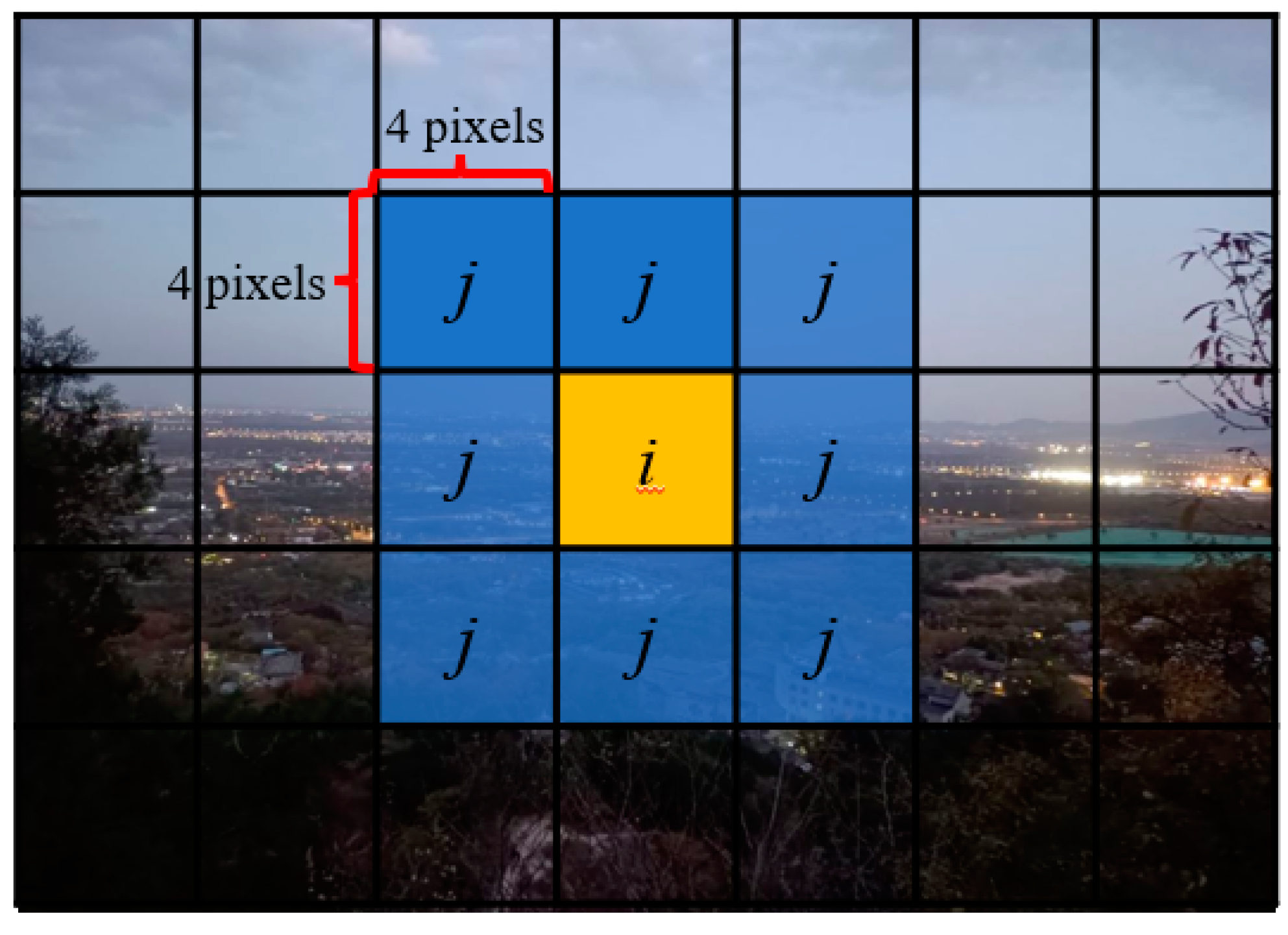
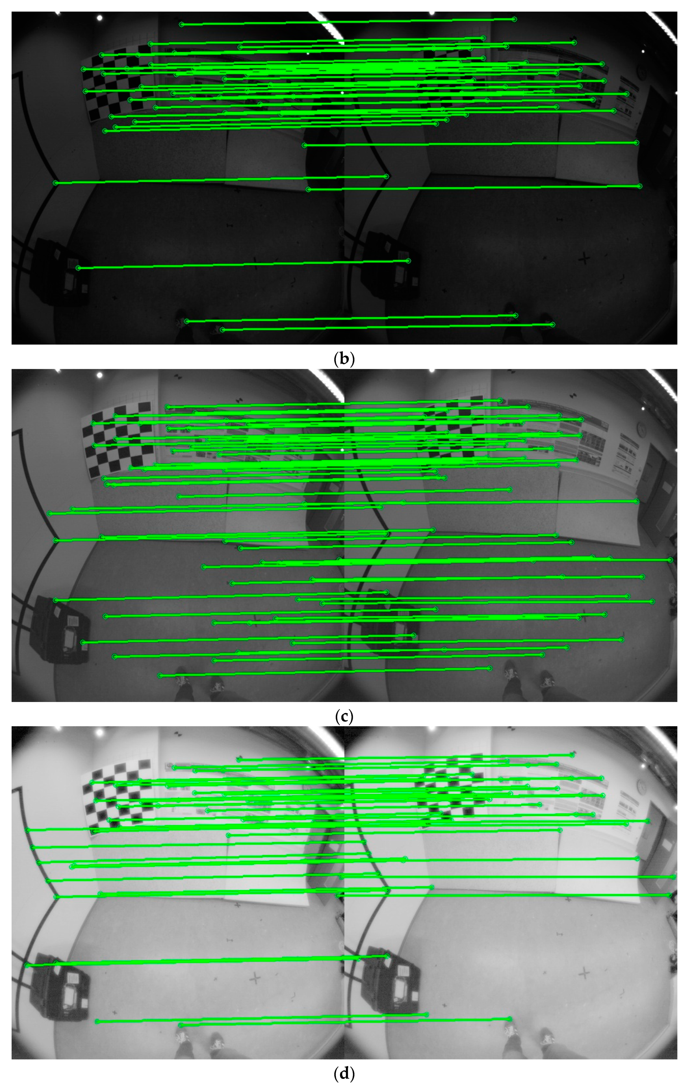
• To satisfy requirements for feature point extraction and matching, we introduce a loss function for spatial consistency. By expanding the measurement range of the spatial consistency loss, texture features are preserved in the regions of the enhanced image, and the stability and repeatability of feature point extraction are improved.
• The proposed image enhancement method is integrated into the VINS-Mono estimator [10] and tested on low-light sequences. Among five evaluated methods, our proposal achieves the minimum positioning error, thus improving the robustness and positioning accuracy of SLAM in low-light environments.

2. Proposed Image Enhancement Method

The proposed low-light image enhancement method is called 3D-DCE++. First, pixelwise transformation curves are estimated using a 3D convolutional neural network (CNN). Then, the transformation curves are iteratively applied to the low-light image to complete enhancement. As shown in Figure 1, the method uses sequential video frames as the input and predicts the grayscale transformation curve parameters of the current frame using the 3D CNN. Then, the iterative process is applied to the current frame to achieve low-light image enhancement. In Section 2.1, we introduce the 2D and 3D convolutions. In Section 2.2, we detail the proposed network structure, loss functions, and iterative enhancement algorithm.

2.1. Two-Dimensional and Three-Dimensional Convolutions

Convolutions can extract features from input data [37]. For a single-step convolution, the convolution kernel parameters and corresponding region of the input data are integrated to calculate their correlation. Then, the convolution result is obtained by adding an offset coefficient and activating using a nonlinear function. By sliding the convolution kernel along a dimension of the input data according to a specific step, the output feature map is obtained depending on the size of the input image, convolution kernel, and sliding step. The number of channels of the output feature map is equal to that of the convolution kernels. If the time dimension is considered, the convolution structure can be divided into 2D and 3D convolutions.

Ji et al. [38] first applied a 3D CNN for human action recognition in surveillance videos. By extracting motion information encoded in the time dimension, the accuracy was notably improved compared with that of a 2D CNN. Tran et al. [39] used a video descriptor trained by a 3D CNN to express spatiotemporal features and achieved excellent performance in four different tasks.

The input in visual SLAM is generally a continuous grayscale image sequence, and the features and textures of adjacent frames are related over time. If only 2D convolutions are applied to an image, temporal information is not fully used, whereas 3D convolutions can extract information from time-series image data. Therefore, we used 3D convolutions in the CNN for low-light enhancement of SLAM image sequences and inferred the corresponding coefficients by using spatiotemporal information to improve the image quality. The 2D and 3D convolutions are described below. Readers can intuitively observe the difference between the 2D and 3D convolutions from the diagrams shown in Figure 2, Figure 3 and Figure 4.

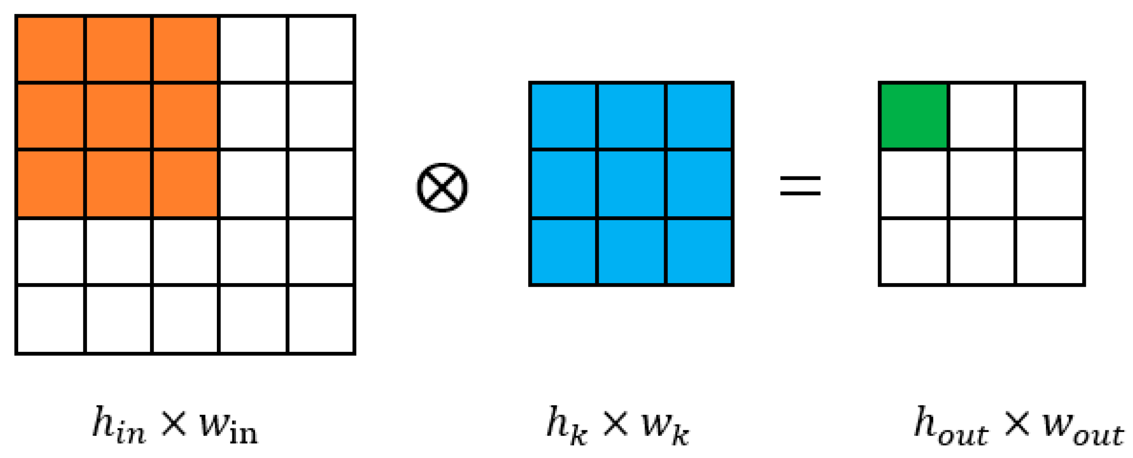
2.1.1. Two-Dimensional Convolution

A one-channel 2D convolution is illustrated in Figure 2, where the highlighted areas indicate one-step calculations and $⨂$ denotes the convolution operation. The input image has size $h_{in}\times w_{in}$, and the $h_k\times w_k$ convolution kernel is slid along the height and width directions, respectively, to obtain a feature map of dimension $h_{out}\times w_{out}$.

When the input data contain multiple channels, a 2D convolution requires the convolution kernel size to be consistent with the number of channels of the input data. Then, each channel is convoluted separately, and the information of each channel is fused into a feature map through summation. The multichannel 2D convolution is illustrated in Figure 3. Let the number of channels, height, and width of the input image be $c_{in}$, $h_{in}$, and $w_{in}$, respectively. The size of a convolution kernel is $c_{in}\times h_k\times w_k$. After sliding the convolution kernel along the direction of the width and height, the output is a feature map of dimension $h_{out}\times w_{out}$.

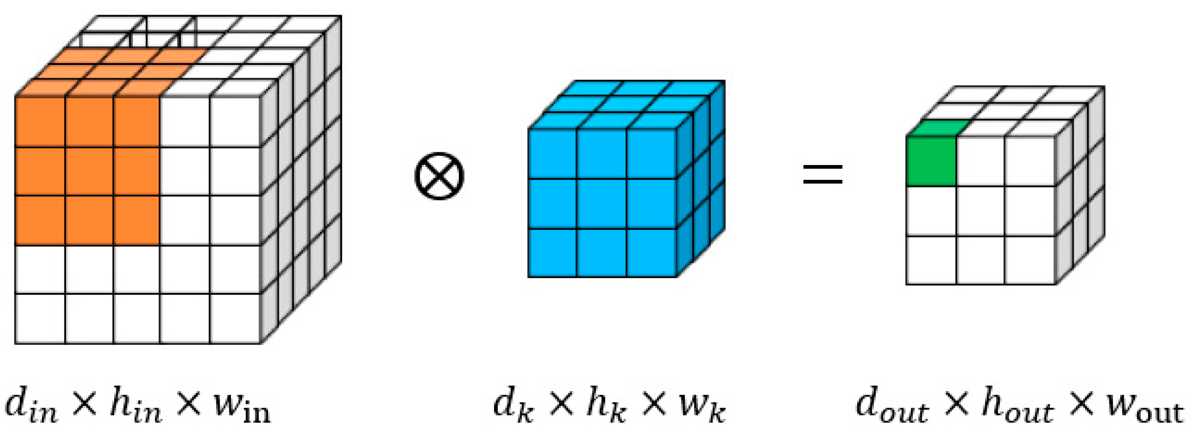
2.1.2. Three-Dimensional Convolution

In addition to sliding along the width and height directions, the 3D convolution kernel slides along the time dimension. When a 3D convolution is applied to time-series data, information regarding the change in the input over time can be extracted. A single-channel 3D convolution is illustrated in Figure 4, where the highlighted areas indicate one-step calculations. For the 3D convolution, the input channels have dimension $d_{in}\times h_{in}\times w_{in}$, where $d_{in}$ denotes the number of frames in the input time series, and the kernel size is $d_k\times h_k\times w_k$, with $d_k$ being the number of frames considered per convolution step, while the output of one kernel has dimension $d_{out}\times h_{out}\times w_{out}$.

2.1.3. Depthwise Separable Convolution

Depthwise convolution is generally applied to reduce the network parameters. For a standard 3D convolution, without considering the bias, the kernel size being $k$, the input channel $c_{in}$, and the output channels $c_{out}$, a depthwise separable convolution factorizes it into a depthwise convolution, which applies a single kernel of size $1\times k\times k\times k$ to each input channel and a pointwise convolution with a kernel of size $c_{in}\times 1\times 1\times 1$ for combining the depthwise convolution output on the depth dimension. The number of pointwise convolution kernels is $c_{out}$. The standard 3D convolution’s parameter number is $c_{in}\times \left(k\times k\times k\times c_{out}\right)$, while the depthwise separable 3D convolution is $c_{in}\times \left(k\times k\times k+c_{out}\right)$.

2.2. 3D-DCE++

In Section 2.2.1, we introduce the structure of the 3D convolutional neural network devised to estimate grayscale transformation curves’ parameters. In Section 2.2.2, we introduce the quadratic curve used for iterative enhancement. Loss functions will be introduced in Section 2.2.3.

2.2.1. Curve Parameter Estimation

The proposed 3D convolutional neural network estimates grayscale transformation curves to be applied to low-light images. The network structure is similar to that of Zero-DCE++. We replaced the 2D depthwise separable convolution layer in Zero-DCE++ with a 3D depthwise separable convolution layer and removed the downsampling layer. Furthermore, we reduced the output channel of the output layer from 3 to 1 due to grayscale images being used in the SLAM system. The proposed 3D convolutional neural network can be divided into encoding and prediction stages. As shown in Figure 5, the encoding stage include Layers 1–6 for feature extraction, and the prediction stage is Layer 7. The input images are N chronological frames of low-light grayscale images. Each layer in the encoding stage performs a 3D depthwise separable convolution with a stride of 1 followed by a rectified linear unit (ReLU) activation. Layer 1 consists of 1 convolution kernel of size $1\times 3\times 3\times 3$ and 32 convolution kernels of size $1\times 1\times 1\times 1$. Layers 2, 3, and 4 consist of 32 convolution kernels of size $1\times 3\times 3\times 3$ and 32 convolution kernels of size $32\times 1\times 1\times 1$. Layers 5 and 6 consist of 64 convolution kernels of size $1\times 3\times 3\times 3$ and 32 convolution kernels of size $64\times 1\times 1\times 1$. The outputs from Layers 3, 2, and 1 pass to Layers 5, 6, and 7 as the inputs through skip connections, respectively. In the prediction stage, 64 convolution kernels of size $1\times 3\times 3\times 3$ and 1 convolution kernel of size $64\times 1\times 1\times 1$ are used in Layer 7 along with hyperbolic tangent activation to estimate the grayscale transformation curve parameter per pixel.

2.2.2. Iterative Enhancement

We used a quadratic curve to enhance the gray value of a low-light image as follows:

$$LE\left(I\left(x\right); \alpha \right)=I\left(x\right)+\alpha I\left(x\right)\left(1-I\left(x\right)\right)$$

(1)

where $x$ denotes the pixel coordinates of the image, $I\left(x\right)$ represents the pixel value of the input low-light image, $I\left(x\right)\in \left[0,1\right]$, $LE\left(I\left(x\right);\alpha \right)$ denotes the pixel value of the enhanced image at $x$, and $\alpha$ is the transformation curve parameter to be estimated for the pixel, with $\alpha \in \left[-1,1\right]$. The iterative process can be expressed as

$$L{E}_n\left(I\left(x\right)\right)=L{E}_{n-1}\left(I\left(x\right)\right)+\mathcal{A}\left(x\right)L{E}_{n-1}\left(I\left(x\right)\right)\left(1-L{E}_{n-1}\left(I\left(x\right)\right)\right)$$

(2)

where $n$ denotes the iteration number and $\mathcal{A}\left(x\right)$ is a parameter matrix of the same size as the input image. We set $n=8$ in this study.

2.2.3. Loss Function

To obtain substantial low-light image enhancement, we used three loss functions based on [35] for training: (1) spatial consistency loss, (2) exposure control loss, and (3) brightness smoothing loss. Because each image in a SLAM sequence has only one channel, the color consistency between channels was not considered.

Feature points used for matching in SLAM often indicate representative regions in an image, and the boundaries between two regions with different local grayscale levels intersect (i.e., textures). Therefore, the original texture information should be preserved in the enhanced image to extract feature points. Zero-DCE++ preserves the texture information through minimizing the difference of four neighboring regions (top, down, left, right) between the input image and its enhanced version. To maintain more spatial consistency in local grayscale levels before and after enhancement, we expanded the spatial consistency loss from four neighboring regions to eight (top, left, down, right, top left, top right, down left, down right). $L_{spa}$ can be formulated as:

$$L_{spa}=\frac{1}{K}{{\displaystyle \sum }}_{i=1}^K{{\displaystyle \sum }}_{j\in \mathsf{\Omega }\left(i\right)}{\left(\left|\left(Y_i-Y_j\right)\right|-\left|\left(I_i-I_j\right)\right|\right)}^2.$$

(3)

where $K$ is the number of surrounding neighboring regions, $\mathsf{\Omega }\left(i\right)$ is a collection of eight neighboring regions around the central region, and $I$ and $Y$ represent the average pixel values of the neighboring region before and after enhancement, respectively. The size of a neighboring region in this study was $4\times 4$. The neighborhood used to calculate the spatial consistency loss is shown in Figure 6. For central region $i$, we selected eight neighbor regions $j$ to calculate the loss.

Overexposure or underexposure can make local areas very bright or dark, respectively. This not only affects the visual appearance of an image, but also makes feature point extraction in these regions difficult and inaccurate. We used exposure control loss $L_{exp}$ to obtain the enhanced image. By splitting an image into non-overlapped fixed-size local regions and minimizing the absolute value of the difference between the local average gray value and the gray value with a good exposure, overexposure or underexposure can be prevented in a local region of the enhanced result:

$$L_{exp}=\frac{1}{M}{{\displaystyle \sum }}_{k=1}^M\left|Y_k-E\right|.$$

(4)

where $M$ is the number of local regions, whose size is $16\times 16$ in this study,$Y$ is the average gray value of the local region, and $E$ is a gray value with good exposure. We empirically set E = 0.45 in this study.

Intuitively, the brightness variation in a high-quality image is smooth, and the variation within smooth regions is small, showing small gradients. Therefore, we smoothed the enhanced image brightness by minimizing the gradient of the parametric feature map along the width and height directions. To this end, we formulate the brightness smoothing loss $L_{tv \mathcal{A}}$ as follows:

$$L_{tv \mathcal{A}}={\left(\left|{\mathsf{\nabla }}_x\mathcal{A}\right|+\left|{\mathsf{\nabla }}_y\mathcal{A}\right|\right)}^2$$

(5)

$\mathcal{A}$ indicates the parameter feature map yielded by the 3D convolutional neural network in Section 2.2.1 and ${\mathsf{\nabla }}_x$ and ${\mathsf{\nabla }}_y$ represent the horizontal and vertical gradient operations, respectively.

The total loss function can be written as

$$L_{total}=L_{spa}+L_{exp}+W_{tv \mathcal{A}}{L}_{tv \mathcal{A}}$$

(6)

where $W_{tv \mathcal{A}}$ is a weight factor used to balance the contributions of the loss functions.

3. Experiments and Results

3.1. Experimental Setup

To avoid overfitting, training data were obtained from a sequence of low-light images in the LLIV-Phone dataset [13], which contains 3072 video frames. The frames were represented in grayscale for training. Low-light image sequences from the TUM-VI public dataset [40] were used to test the effect of the model on the positioning improvement. A frame and the preceding one were used for training, and we set the batch size to eight, the optimizer to the Adam method, the learning rate to 0.0001, and the weight decay to 0.0001. We initialized all the convolutional layer parameters using a Gaussian distribution with zero mean and a standard deviation of 0.02. We directly trained our network on low-light image sequences from the LLIV-Phone dataset without paired reference images. The weight factor $W_{tv \mathcal{A}}$ was set to 100 to balance the scale of loss. Owing to the lightweight network structure, we achieved real-time operation without requiring downsampling of the input image. For a fair comparison, we also removed the downsampling layer of Zero-DCE++’s performance during the experiments due to the fact that downsampling may be detrimental to spatial consistency. For the experiments, we used a computer equipped with an Intel Core i7-11800H processor, NVIDIA 3060 graphics card, and 16 GB memory. The computer was running the Ubuntu 20.04 operating system.

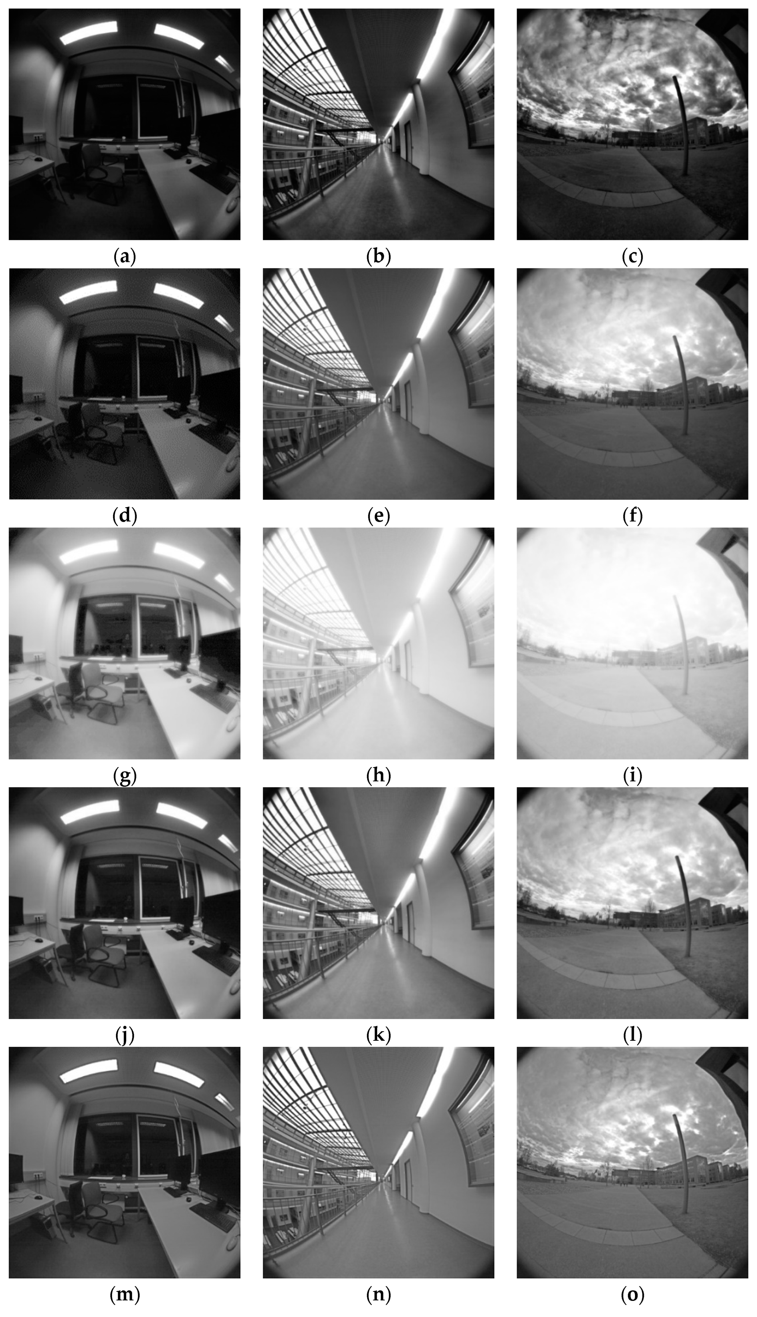
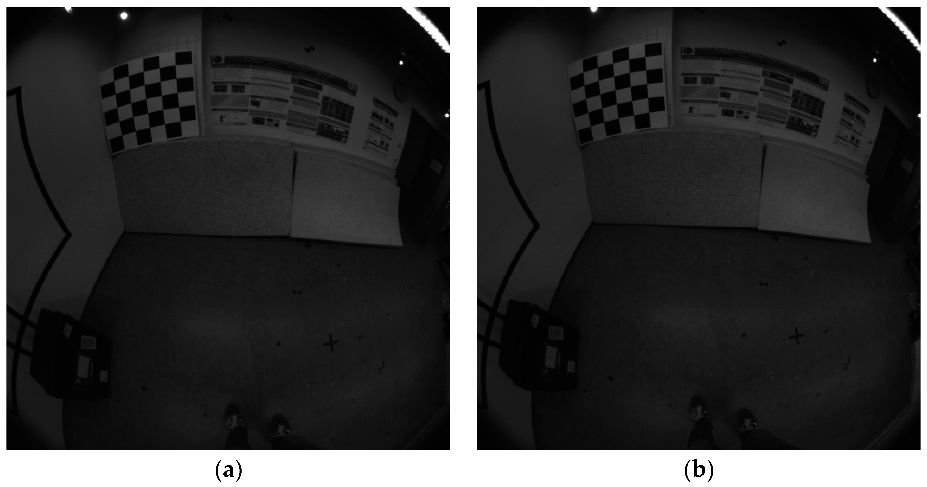
3.2. Low-Light Image Enhancement

We qualitatively compared the results of low-light image enhancement for individual frames and quantitatively compared the real-time operation of five evaluated methods: CLAHE, GC, SSR, Zero-DEC++, and the proposed 3D-DCE++.

The low-light images selected for qualitative comparison were extracted from sequences in the TUM-VI public dataset, which contains both indoor and outdoor scenes. This dataset was designed to assess the positioning accuracy of a visual inertial navigation system comprising a binocular camera and IMU data. The dataset provides images with 512 × 512 and 1024 × 1024 resolution at 20 Hz, which was acquired using UI-3241LE-M-GL fisheye cameras. The IMU measured the acceleration and angular velocity along the three axes at 200 Hz. The camera and IMU were time synchronized by hardware. The dataset has 28 different sequences from different scenes, such as rooms, corridors, outdoors, and slides.

We selected a set of sample images from different dataset sequences to test the enhancement effect of low-light images. The selected samples are shown in Figure 7 and include indoor, corridor, and outdoor scenes. The brightness of the three images is low, and there are varying degrees of uneven lighting and low contrast.

We applied the evaluated methods to enhance the images in Figure 6, obtaining the enhancement results shown in Figure 8.

Figure 8 shows that Zero-DCE++ and 3D-DCE++ considerably outperformed the conventional methods regarding visual quality. The brightness of low-light regions was enhanced while retaining bright areas, and the overall image quality improved. CLAHE and GC, which limit the contrast, can enhance the brightness in the middle region of the image, but the brightness of the image in the four corners remained low. As a result, the contrast between chairs and ground in Figure 8a,d is low. Although SSR improved the brightness, it was very high, while the processing result was blurry, and the image was not smooth, resulting in an unrealistic scene. Zero-DCE++ enhanced the overall image, but it failed to reflect some details, such as the texture-rich area on the left side in the second corridor scene, which is noisy and blurry. In general, the proposed 3D-DCE++ showed the best enhancement effect for low-light images.

We also evaluated the computation time of each method. The average computation time was obtained by repeating the experiments on sequences from the TUM-VI dataset. The input for all the methods was a 512 × 512-pixel grayscale image. The test results are listed in

Table 1. Computation time of evaluated low-light image enhancement methods.

Method	Computation Time per Frame (s)
CLAHE	0.000150
GC	0.000800
SSR	0.032917
Zero-DCE++	0.012503
3D-DCE++ (Ours)	0.015070

.

Table 1 suggests the real-time operation of the proposed 3D-DCE++, with a computation time per frame of 0.015107 s. In fact, our method can achieve a real-time processing frequency of 90 Hz, while most cameras capture images at 20 or 30 Hz, indicating its suitability for SLAM. Compared with Zero-DCE++, the computation time of our method was similar despite using 3D convolutions, and we achieved a lower positioning error. Owing to its lightweight network, 3D-DCE++ was faster than the conventional SSR.

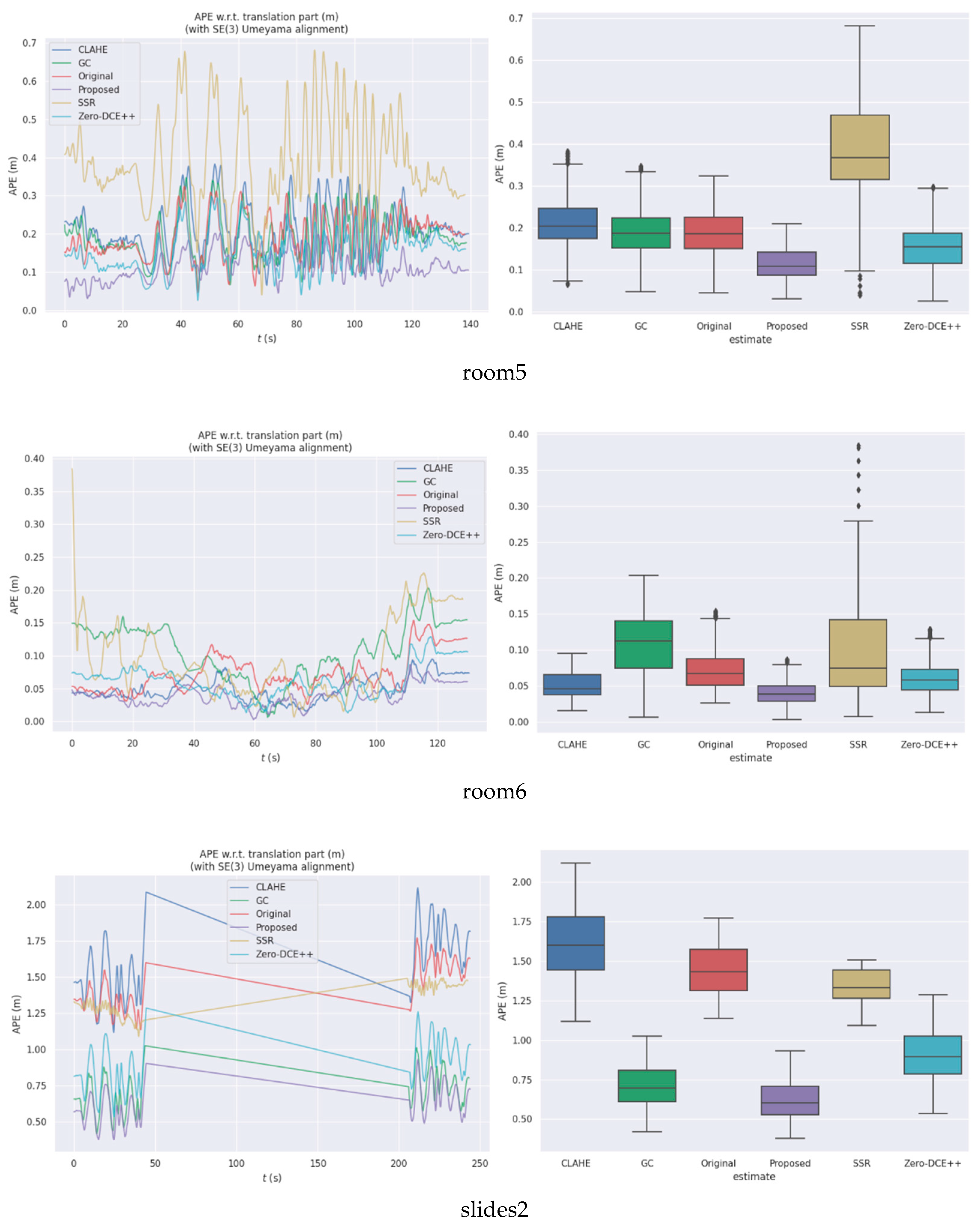
3.3. Sequence Positioning Error

Considering varying lighting conditions in different scenes, we conducted experiments to evaluate the method robustness. Seven low-light image sequences (i.e., corridor1, corridor5, room1, room2, room5, room6, and slides2) were selected from the TUM-VI dataset for evaluation. Corridor1 and corridor5 are sequences in the corridor and several offices at night. The camera’s movement in the corridor and different rooms make the grayscale level of the image change in a high dynamic range. Room1, room2, room5, and room6 are sequences in office rooms at night, and the camera revolves around the room. In addition to offices and corridors, sequence slides2 also contains a closed tube with very bad illumination inside. Slides2’s environment also contains much glass, which will refract light and then affect the brightness of the image. Therefore, the above sequence contains different lighting conditions, which helps to test the robustness of the algorithm to different dark scenes.

We selected two adjacent frames to compare feature matching results after applying different low-light image enhancement methods. Figure 9 shows the original images. Figure 9a is the previous frame, and Figure 9b is the current frame. During the experiment, the system performed feature point extraction, outlier elimination, and feature matching. We integrated different low-light image enhancement methods into the open-source VINS-Mono estimator [10].

Figure 10 shows the results of feature matches for the two image frames. In Figure 9a, barely any feature points are extracted from the low-light area in the middle of the image. Comparing Figure 10a–d, we see that while the number of feature points and matches increased after applying CLAHE, GC, and SSR to the original low-light image, they were still less than those in the enhanced results using the proposed method. Comparing Figure 9a,b and Figure 10d, we can see that the enhanced results of SSR are more blurred than the original images. It discarded the texture information of the original image, which is unfavorable to the repeated extraction of feature points. Comparing Figure 10e,f, we can see that the proposed method obtained more feature points and matches on some local area owing to our 3D convolution module and spatial consistency loss function. Therefore, when the camera is disturbed by a low-light environment, our method can enhance the low-light image sequence and obtain better feature matches.

We integrated different low-light image enhancement methods into the open-source VINS-Mono estimator [10] for SLAM to measure the positioning accuracy. The root-mean-squared error (RMSE) of the absolute positioning error was used to measure the positioning accuracy, and the Evo open-source library [41] was used for the calculations. Because the coordinate systems of the system position and real track estimated by the algorithm differ, they should be aligned first. We used SE(3) Umeyara alignment to align the trajectory of the experimental results to the ground truth. After calculating transformation matrix $S\in \mathrm{SE}\left(3\right)$ from the coordinate system of the experimental results to the real track coordinate system using the least-squares method, the absolute positioning error of frame i can be calculated as follows [42]:

$$E_i=Q_i{}^{-1}S{P}_i$$

(7)

where $E$, $Q$, $S$, and $P$ are transformation matrices that contain both position shift and rotation posture information. They are expressed as $\left[\begin{array}{cc}R& t\\ 0^T& 1\end{array}\right]$, where $R$ is the rotation matrix and $t$ is the translation vector. For frame i, $E_i$ represents the absolute positioning error, $Q_i$ represents the true track, and $P_i$ represents the estimated pose.

Then, the absolute positioning error and its RMSE can be calculated as follows:

$$RMSE\left(E_{1:n},\Delta \right)={\left(\frac{1}{m}{{\displaystyle \sum }}_{i=1}^m{\Vert trans\left(E_i\right)\Vert }^2\right)}^{\frac{1}{2}}.$$

(8)

where $\Delta$ is a time interval, $m$ is the number of samples, and $trans\left(T\right)$ represents the shift information in transformation matrix $T$, that is shift vector t.

The calculated RMSE values of the experimental results for the evaluated methods in seven sequences were calculated, obtaining the results listed in

Table 2. Positioning errors (in meters) in low-light image sequences using VINS-Mono after applying the evaluated image enhancement methods.

Sequence	Original	CLAHE	GC	SSR	Zero-DCE++	3D-DCE++ (Ours)	Compared with Zero-DCE++
corridor1	2.3635	0.4137	0.7454	5.0429	0.4667	0.3913	16.15%
corridor5	0.3557	0.5608	0.6721	0.7177	0.3177	0.2547	19.83%
room1	0.0875	0.0521	0.0671	0.1212	0.0396	0.0395	0.18%
room2	0.1246	0.0792	0.1200	0.1571	0.0823	0.0696	15.38%
room5	0.1979	0.2224	0.2002	0.4092	0.1646	0.1215	26.18%
room6	0.0795	0.0532	0.1160	0.1130	0.0662	0.0423	36.18%
slides2	1.4485	0.6215	0.7181	1.3489	0.9114	0.6313	30.73%

. The values in boldface indicate the smallest positioning error and highest positioning accuracy for every sequence. The last column of the table provides the accuracy improvement of the proposed 3D-DCE++ compared with the Zero-DCE++ algorithm based on deep learning, which is calculated as follows:

$$\gamma =\left(1-\frac{\delta }{\epsilon }\right)\times 100\%$$

(9)

where $\gamma$ is the percentage of RMSE improvement, $\delta$ is the RMSE of the proposed 3D-DCE++, and $\epsilon$ is the RMSE of Zero-DCE ++.

Table 2 shows that, compared with directly extracting feature points on the original images with the VINS-Mono estimator, using the low-light image enhancement methods can improve the positioning accuracy to some extent. The positioning error provided by the proposed 3D-DCE++ was the smallest, while the positioning accuracy was the highest, indicating a substantial improvement. Compared with Zero-DCE++ using 2D convolutions, 3D-DCE++ had a median reduction of 19.83% in the RMSE of the absolute positioning error in the seven sequences.

The statistical results of the absolute positioning errors are shown in Figure 11. The left images denote the positioning error versus time. The abscissa is the system’s runtime in seconds, while the ordinate is the system’s absolute position error in meters. The right images are the boxplot of the five methods. The abscissa is the six low-light image enhanced methods applied in the SLAM system (including original), while the ordinate is the system’s absolute position error in meters.

For corridor1 and corridor5, the proposed method and Zero-DCE++ had higher accuracy compared with the other three methods, and the positioning accuracy of the proposed method was slightly higher. For room5, room6, and slides2, the median and variance of the proposed method’s absolute error were both the smallest. For slides2, Zero-DCE++’s positioning accuracy was lower than the conventional method GC. For corridor1, corridor5, room1, room2, room5, and room6, SSR could not improve the positioning accuracy.

In summary, the proposed method achieved the best performance in different scenarios, which proves the generality and robustness of the proposed method.

4. Discussion

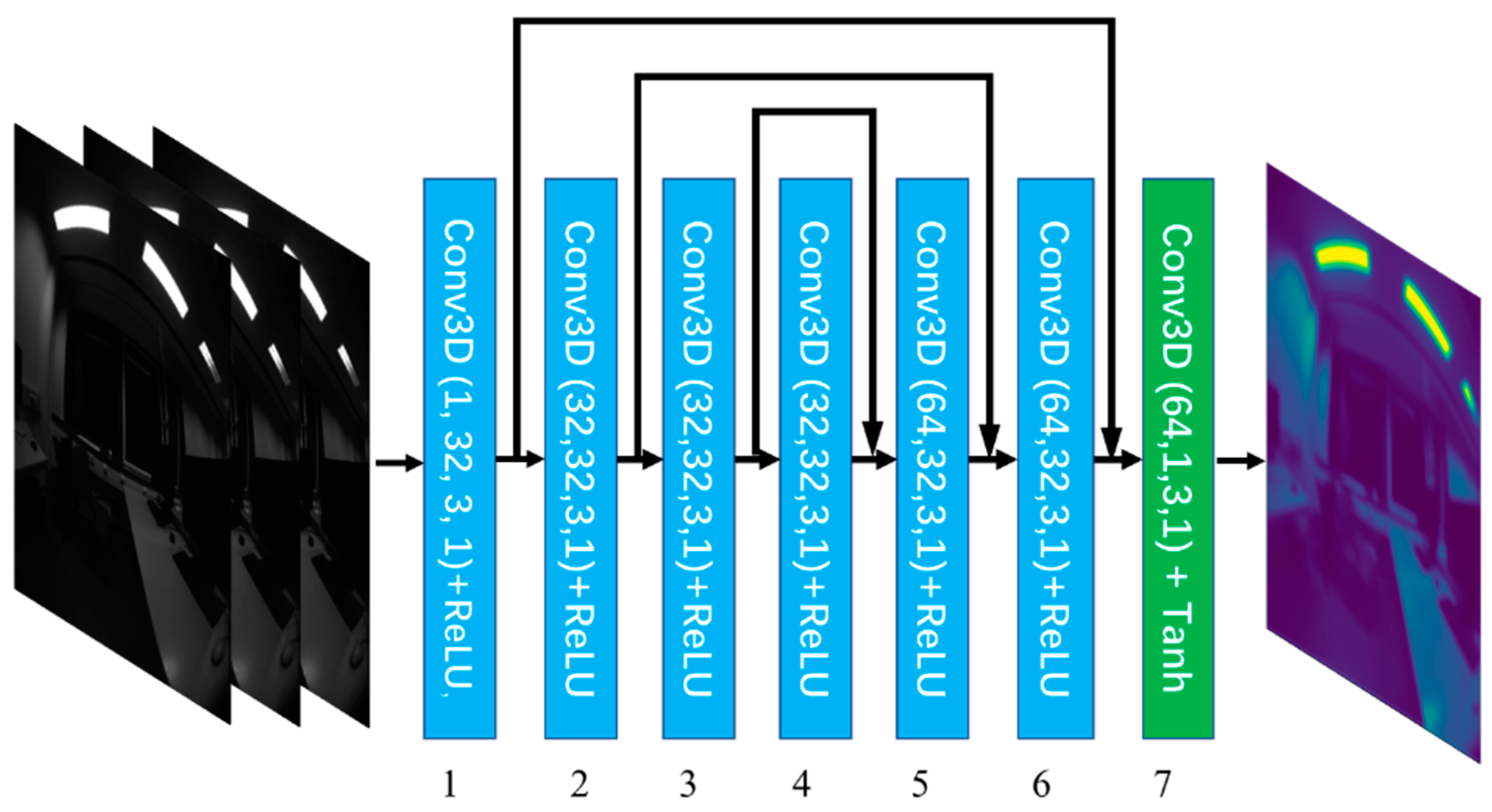
• Deep-learning-based methods have recently attracted significant attention in the SLAM research field. Due to the powerful feature representation ability of the data, a deep neural network can learn more general visual features. This property means a deep learning model can be used to relieve some challenges for geometry-based visual odometry, such as featureless areas, dynamic lighting conditions, and motion blur. Our research is aimed at combining the deep-learning-based low-light image enhancement methods with geometry-based visual odometry to improve the robustness of the visual SLAM system in a low-light environment. Zero-DCE++ employs zero-reference learning and a lightweight network to complete the low-light image enhancement task. These characteristics offer Zero-DCE++ the advantages of a flexible generalization capability and real-time inference speed. Moreover, we notice that the input data of the visual SLAM system have a strong temporal correlation. The ability to analyze a series of frames in context led to 3D convolution being used as a tool for spatiotemporal feature extractors in video analytics research. Therefore, we replaced the 2D convolution with 3D convolution to extract the temporal feature of the input image sequence. To improve the stability of feature point extraction, we abandoned the downsampling operation and strengthened the spatial consistency constraint. To evaluate the proposed method, we integrated different methods into VINS-Mono and compared their positioning error.
• The quantitative results in Table 2 show that both learning-based methods reduce the system’s positioning error on all sequences, while traditional methods increase positioning error on some sequences. We considered that the main reason may be that the parameters for image enhancement of traditional methods are fixed, while Zero-DCE++ and our method are constantly changing according to the input images. This also proves that the proposed method generalizes well to different lighting conditions.
• To analyze the computational complexity and model complexity increase by 3D convolution, we calculated the floating-point operations (FLOPs) and the number of parameters of Zero-DCE++ and our method. Following Section 3.2 and Section 3.3, we used the original size of the input image to calculate the FLOPs of Zero-DCE++ without downsampling. For an input image of size $512\times 512$, the FLOPs and trainable parameters of the two methods are shown in

  Table 3. The comparison of computational complexity and number of parameters.

  Method	FLOPs	Number of Parameters
  Zero-DCE++	2.65G	10k
  Ours	7.89G	15k

  . As shown in Table 3, the costs of introducing 3D convolution into Zero-DCE++ are that the FLOPs increased by two times and the number of parameters increased to 15K. Thankfully, for 15k, 7.89G FLOPs of 3D-DCE++ is still smaller than the technical specifications of existing NVIDIA edge platforms (Jetson Nano 4GB, 472G FLOPs; Jetson TX2: 8GB, 1.3T FLOPs) [43,44]. The proposed method can be deployed on specialized embedded devices.

5. Conclusions

To improve the imaging quality of low-light scenes, reduce information loss in images, and improve the positioning accuracy of the SLAM system in low-light environments, we proposed a low-light image enhancement method for image sequences used in visual SLAM based on [35]. Because the input for visual SLAM is a video sequence, we considered the spatiotemporal characteristics of a sequence. Spatiotemporal features of image sequences can be extracted using 3D convolutions. In addition, spatial consistency in the enhanced image pixels is preserved using the corresponding loss function, and the stability of feature point tracking and extraction is improved. The proposed 3D-DCE++ was integrated into the VINS-Mono estimator and evaluated on the TUM-VI public dataset. Experimental results demonstrated that our method improves the visual quality of low-light images. Moreover, a comparison with the ground truth shows that for different scenes and lighting conditions, the SLAM system’s positioning accuracy is improved using 3D-DCE++, which achieves the smallest positioning error and highest positioning accuracy among various evaluated methods. We believe that 3D-DCE++ can improve SLAM even in more challenging scenes.

In the future, we plan to integrate semantic information into image sequence enhancement and design a more light-weight 3D CNN architecture. By combining more prior constraints and reducing the computational cost, further accuracy gains in location and more practical applications are achievable.

References

1. Nguyen, H.; Mascarich, F.; Dang, T.; Alexis, K. Autonomous aerial robotic surveying and mapping with application to construction operations. arXiv 2020, arXiv:2005.04335. [Google Scholar] [CrossRef]
2. Liu, Z.; Di, K.; Li, J.; Xie, J.; Cui, X.; Xi, L.; Wan, W.; Peng, M.; Liu, B.; Wang, Y.; et al. Landing site topographic mapping and rover localization for Chang’e-4 mission. Sci. China Inf. Sci. 2020, 63, 140901. [Google Scholar] [CrossRef]
3. Chen, X.; Zhang, H.; Lu, H.; Xiao, J.; Qiu, Q.; Li, Y. Robust SLAM System based on Monocular Vision and LiDAR for Robotic Urban Search and Rescue. In Proceedings of the 2017 IEEE International Symposium on Safety, Security and Rescue Robotics (SSRR), Shanghai, China, 11–13 October 2017; pp. 41–47. [Google Scholar] [CrossRef]
4. Chiang, K.-W.; Tsai, G.-J.; Li, Y.-H.; Li, Y.; El-Sheimy, N. Navigation engine design for automated driving using INS/GNSS/3D LiDAR-SLAM and integrity assessment. Remote Sens. 2020, 12, 1564. [Google Scholar] [CrossRef]
5. Kaichang, D.I.; Wenhui, W.A.; Hongying, Z.H.; Zhaoqin, L.I.; Runzhi, W.A.; Feizhou, Z.H. Progress and applications of visual SLAM. Acta Geod. Cartogr. Sin. 2018, 47, 770. [Google Scholar] [CrossRef]
6. Cadena, C.; Carlone, L.; Carrillo, H.; Latif, Y.; Scaramuzza, D.; Neira, J.; Reid, I.D.; Leonard, J.J. Simultaneous localization and mapping: Present, future, and the robust-perception age. IEEE Trans. Robot. 2016, 32, 1309–1332. [Google Scholar] [CrossRef]
7. Davison, A.J.; Reid, I.D.; Molton, N.D.; Stasse, O. MonoSLAM: Real-time single camera SLAM. IEEE Trans. Pattern Anal. Mach. Intell. 2007, 29, 1052–1067. [Google Scholar] [CrossRef]
8. Hartley, R.; Zisserman, A. Multiple View Geometry in Computer Vision; Cambridge University Press: Cambridge, UK, 2003. [Google Scholar]
9. Nützi, G.; Weiss, S.; Scaramuzza, D.; Siegwart, R.J. Fusion of IMU and vision for absolute scale estimation in monocular SLAM. J. Intell. Robot. Syst. 2011, 61, 287–299. [Google Scholar] [CrossRef]
10. Qin, T.; Li, P.; Shen, S. Vins-mono: A robust and versatile monocular visual-inertial state estimator. IEEE Trans. Robot. 2018, 34, 1004–1020. [Google Scholar] [CrossRef]
11. Campos, C.; Elvira, R.; Rodríguez, J.J.G.; Montiel, J.M.; Tardós, J.D. ORB-SLAM3: An accurate open-source library for visual, visual–inertial, and multimap SLAM. IEEE Trans. Robot. 2021, 37, 1874–1890. [Google Scholar] [CrossRef]
12. Mourikis, A.I.; Roumeliotis, S.I. A Multi-State Constraint Kalman Filter for Vision-Aided Inertial Navigation. In Proceedings of the 2007 IEEE International Conference on Robotics and Automation, Roma, Italy, 10–14 April 2007; pp. 3565–3572. [Google Scholar] [CrossRef]
13. Li, C.; Guo, C.; Han, L.-H.; Jiang, J.; Cheng, M.-M.; Gu, J.; Loy, C.C. Low-light image and video enhancement using deep learning: A survey. IEEE Trans. Pattern Anal. Mach. Intell. 2021. [Google Scholar] [CrossRef]
14. Harris, C.; Stephens, M. A Combined Corner and Edge Detector. In Proceedings of the Alvey Vision Conference, Manchester, UK, 31 August–2 September 1988; pp. 147–151. [Google Scholar]
15. Lowe, D.G. Distinctive image features from scale-invariant keypoints. Int. J. Comput. Vis. 2004, 60, 91–110. [Google Scholar] [CrossRef]
16. Rublee, E.; Rabaud, V.; Konolige, K.; Bradski, G. ORB: An Efficient Alternative to SIFT or SURF. In Proceedings of the 2011 International Conference on Computer Vision, Barcelona, Spain, 6–13 November 2011; pp. 2564–2571. [Google Scholar] [CrossRef]
17. Abdullah-Al-Wadud, M.; Kabir, M.H.; Dewan, M.A.A.; Chae, O. A dynamic histogram equalization for image contrast enhancement. IEEE Trans. Consum. Electron. 2007, 53, 593–600. [Google Scholar] [CrossRef]
18. Ibrahim, H.; Kong, N.S. Brightness preserving dynamic histogram equalization for image contrast enhancement. IEEE Trans. Consum. Electron. 2007, 53, 1752–1758. [Google Scholar] [CrossRef]
19. Pisano, E.D.; Zong, S.; Hemminger, B.M.; DeLuca, M.; Johnston, R.E.; Muller, K.; Braeuning, M.P.; Pizer, S.M. Contrast limited adaptive histogram equalization image processing to improve the detection of simulated spiculations in dense mammograms. J. Digit. Imaging 1998, 11, 193–200. [Google Scholar] [CrossRef]
20. Jeong, I.; Lee, C. An optimization-based approach to gamma correction parameter estimation for low-light image enhancement. Multimed. Tools Appl. 2021, 80, 18027–18042. [Google Scholar] [CrossRef]
21. Li, C.; Tang, S.; Yan, J.; Zhou, T. Low-light image enhancement based on quasi-symmetric correction functions by fusion. Symmetry 2020, 12, 1561. [Google Scholar] [CrossRef]
22. Xu, Q.; Jiang, H.; Scopigno, R.; Sbert, M. A novel approach for enhancing very dark image sequences. Signal Process. 2014, 103, 309–330. [Google Scholar] [CrossRef]
23. Land, E.H. The retinex theory of color vision. Sci. Am. 1977, 237, 108–129. [Google Scholar] [CrossRef]
24. Parihar, A.S.; Singh, K. A Study on Retinex Based Method for Image Enhancement. In Proceedings of the 2018 2nd International Conference on Inventive Systems and Control (ICISC), Coimbatore, India, 19–20 January 2018; pp. 619–624. [Google Scholar] [CrossRef]
25. Zotin, A. Fast algorithm of image enhancement based on multi-scale retinex. Procedia Comput. Sci. 2018, 131, 6–14. [Google Scholar] [CrossRef]
26. Fu, X.; Zeng, D.; Huang, Y.; Zhang, X.-P.; Ding, X. A Weighted Variational Model for Simultaneous Reflectance and Illumination Estimation. In Proceedings of the IEEE Conference on Computer Vision and Pattern Recognition (CVPR), Salt Lake City, UT, USA, 18–23 June 2018; pp. 2782–2790. [Google Scholar] [CrossRef]
27. Li, M.; Liu, J.; Yang, W.; Sun, X.; Guo, Z. Structure-revealing low-light image enhancement via robust retinex model. IEEE Trans. Image Process. 2018, 27, 2828–2841. [Google Scholar] [CrossRef]
28. Lore, K.G.; Akintayo, A.; Sarkar, S. LLNet: A deep autoencoder approach to natural low-light image enhancement. Pattern Recognit. 2017, 61, 650–662. [Google Scholar] [CrossRef]
29. Lv, F.; Lu, F.; Wu, J.; Lim, C. MBLLEN: Low-Light Image/Video Enhancement Using CNNs. In Proceedings of the 29th British Machine Vision Conference (BMVC), Northumbria University, Newcastle, UK, 3–6 September 2018; p. 4. [Google Scholar]
30. Wei, C.; Wang, W.; Yang, W.; Liu, J.J. Deep retinex decomposition for low-light enhancement. arXiv 2018, arXiv:1808.04560. [Google Scholar]
31. Zhang, Y.; Guo, X.; Ma, J.; Liu, W.; Zhang, J. Beyond brightening low-light images. Int. J. Comput. Vis. 2021, 129, 1013–1037. [Google Scholar] [CrossRef]
32. Ren, W.; Liu, S.; Ma, L.; Xu, Q.; Xu, X.; Cao, X.; Du, J.; Yang, M.-H. Low-light image enhancement via a deep hybrid network. IEEE Trans. Image Process. 2019, 28, 4364–4375. [Google Scholar] [CrossRef] [PubMed]
33. Zhang, L.; Zhang, L.; Liu, X.; Shen, Y.; Zhang, S.; Zhao, S. Zero-Shot Restoration of Back-Lit Images Using Deep Internal Learning. In Proceedings of the 2019 ACM International Conference on Multimedia (ACMMM), Nice, France, 21–25 October 2019; pp. 1623–1631. [Google Scholar] [CrossRef]
34. Guo, C.; Li, C.; Guo, J.; Loy, C.C.; Hou, J.; Kwong, S.; Cong, R. Zero-Reference Deep Curve Estimation for Low-Light Image Enhancement. In Proceedings of the 2020 IEEE/CVF Conference on Computer Vision and Pattern Recognition (CVPR), Virtual, 14–19 June 2020; pp. 1780–1789. [Google Scholar]
35. Li, C.; Guo, C.; Loy, C.C. Learning to enhance low-light image via zero-reference deep curve estimation. arXiv 2021, arXiv:2103.00860. [Google Scholar] [CrossRef]
36. Szegedy, C.; Liu, W.; Jia, Y.; Sermanet, P.; Reed, S.; Anguelov, D.; Erhan, D.; Vanhoucke, V.; Rabinovich, A. Going Deeper with Convolutions. In Proceedings of the 2015 the IEEE/CVF Conference on Computer Vision and Pattern Recognition (CVPR), Boston, MA, USA, 7–12 June 2015; pp. 1–9. [Google Scholar]
37. LeCun, Y.; Bottou, L.; Bengio, Y.; Haffner, P. Gradient-based learning applied to document recognition. Proc. IEEE 1998, 86, 2278–2324. [Google Scholar] [CrossRef]
38. Ji, S.; Xu, W.; Yang, M.; Yu, K. 3D convolutional neural networks for human action recognition. IEEE Trans. Pattern Anal. Mach. Intell. 2012, 35, 221–231. [Google Scholar] [CrossRef]
39. Tran, D.; Bourdev, L.; Fergus, R.; Torresani, L.; Paluri, M. Learning Spatiotemporal Features with 3D Convolutional Networks. In Proceeding of the 2015 IEEE International Conference on Computer Vision (ICCV), Santiago, Chile, 13–16 December 2015; pp. 4489–4497. [Google Scholar]
40. Schubert, D.; Goll, T.; Demmel, N.; Usenko, V.; Stückler, J.; Cremers, D. The TUM VI Benchmark for Evaluating Visual-Inertial Odometry. In Proceedings of the 2018 IEEE/RSJ International Conference on Intelligent Robots and Systems (IROS), Madrid, Spain, 1–5 October 2018; pp. 1680–1687. [Google Scholar] [CrossRef]
41. Grupp, M. Evo: Python Package for the Evaluation of Odometry and SLAM; 2017. Available online: http://github.com/MichaelGrupp/evo (accessed on 1 July 2022).
42. Sturm, J.; Engelhard, N.; Endres, F.; Burgard, W.; Cremers, D. A Benchmark for the Evaluation of RGB-D SLAM Systems. In Proceedings of the 2012 IEEE/RSJ International Conference on Intelligent Robots and Systems (IROS), Algarve, Portugal, 7–12 October 2012; pp. 573–580. [Google Scholar] [CrossRef]
43. Süzen, A.A.; Duman, B.; Şen, B. Benchmark Analysis of Jetson tx2, Jetson Nano and Raspberry pi Using Deep-cnn. In Proceedings of the 2020 International Congress on Human-Computer Interaction, Optimization and Robotic Applications (HORA), Ankara, Turkey, 26–28 June 2020; pp. 1–5. [Google Scholar]
44. Ullah, S.; Kim, D.-H. Benchmarking Jetson platform for 3D Point-Cloud and Hyper-Spectral Image Classification. In Proceedings of the 2020 IEEE International Conference on Big Data and Smart Computing (BigComp), Busan, Korea, 19–22 February 2020; pp. 477–482. [Google Scholar]
Figure 1. Framework of the proposed 3D-DCE++ based on Zero-DCE++ in [35]. 3D-DCE++ can be divided into two stages. First, a 3D convolutional neural network is proposed to estimate the grayscale transformation curves’ parameters. Then, the framework maps all pixels of the input current frame into the final enhanced image by applying the curve iteratively. I represent the original input low-light image; L E n denotes the enhanced image of nth iteration; A denotes the curve parameter feature map with the same size of the input image.
Remotesensing 14 03985 g001
Figure 2. Diagram of one-channel 2D convolution.
Remotesensing 14 03985 g002
Figure 3. Diagram of multichannel 2D convolution.
Remotesensing 14 03985 g003
Figure 4. Diagram of single-channel 3D convolution.
Remotesensing 14 03985 g004
Figure 5. Architecture of the proposed 3D CNN. Conv3D, depthwise separable 3D convolution; ReLU, rectified linear unit; Tanh, hyperbolic tangent. The layer number is annotated at the bottom. Layers 1–6 in blue belong to the encoder stage, and Layer 7 in green belongs to the prediction stage.
Remotesensing 14 03985 g005
Figure 6. Diagram of calculating spatial consistency loss.
Remotesensing 14 03985 g006
Figure 7. Samples from the TUM-VI public dataset to evaluate low-light image enhancement in (a) indoor, (b) corridor, and (c) outdoor scenes.
Remotesensing 14 03985 g007
Figure 8. Low-light image enhancement of samples from the TUM-VI dataset (Figure 6) using (ac) CLAHE, (df) GC, (gi) SSR, (jl) Zero-DCE++, and (mo) the proposed 3D-DCE++.
Remotesensing 14 03985 g008
Figure 9. Low-light image data of two adjacent frames in slides2. (a) Previous frame. (b) Current frame.
Remotesensing 14 03985 g009
Figure 10. Feature point matching results of adjacent frames (Figure 8) using the (a) original, (b) CLAHE, (c) GC, (d) SSR, (e) Zero-DCE++, and (f) proposed 3D-DCE++.
Remotesensing 14 03985 g010aRemotesensing 14 03985 g010bRemotesensing 14 03985 g010c
Figure 11. Comparison of the positioning errors of VINS-Mono using CLAHE, GC, SSR, Zero-DCE++, and the proposed method on different low-light image sequences. The first column is the absolute positioning error distribution over time, and the second column is the boxplot of the above methods.
Remotesensing 14 03985 g011aRemotesensing 14 03985 g011b