Exploring Transferable Techniques to Retrieve Crop Biophysical and Biochemical Variables Using Sentinel-2 Data

Abstract

The current study aimed to determine the spatial transferability of eXtreme Gradient Boosting (XGBoost) models for estimating biophysical and biochemical variables (BVs), using Sentinel-2 data. The specific objectives were to: (1) assess the effect of different proportions of training samples (i.e., 25%, 50%, and 75%) available at the Target site (${\mathcal{D}}_T$) on the spatial transferability of the XGBoost models and (2) evaluate the effect of the Source site (${\mathcal{D}}_S$) (i.e., trained) model accuracy on the Target site (i.e., unseen) retrieval uncertainty. The results showed that the Bothaville (${\mathcal{D}}_S$) → Harrismith (${\mathcal{D}}_T$) Leaf Area Index (LAI) models required only fewer proportions, i.e., 25% or 50%, of the training samples to make optimal retrievals in the ${\mathcal{D}}_T$ (i.e., RMSE: 0.61 m² m⁻²; R²: 59%), while Harrismith (${\mathcal{D}}_S$) →Bothaville (${\mathcal{D}}_T$) LAI models required up to 75% of training samples in the ${\mathcal{D}}_T$ to obtain optimal LAI retrievals (i.e., RMSE = 0.63 m² m⁻²; R² = 67%). In contrast, the chlorophyll content models for Bothaville (${\mathcal{D}}_S$) → Harrismith (${\mathcal{D}}_T$) required significant proportions of samples (i.e., 75%) from the ${\mathcal{D}}_T$ to make optimal retrievals of Leaf Chlorophyll Content (LC_ab) (i.e., RMSE: 7.09 µg cm⁻²; R²: 58%) and Canopy Chlorophyll Content (CCC) (i.e., RMSE: 36.3 µg cm⁻²; R²: 61%), while Harrismith (${\mathcal{D}}_S$) →Bothaville (${\mathcal{D}}_T$) models required only 25% of the samples to achieve RMSEs of 8.16 µg cm⁻² (R²: 83%) and 40.25 µg cm⁻² (R²: 77%), for LC_ab and CCC, respectively. The results also showed that the source site model accuracy led to better transferability for LAI retrievals. In contrast, the accuracy of LC_ab and CCC source site models did not necessarily improve their transferability. Overall, the results elucidate the potential of transferable Machine Learning Regression Algorithms and are significant for the rapid retrieval of important crop BVs in data-scarce areas, thus facilitating spatially-explicit information for site-specific farm management.

1. Introduction

Accurate and reliable estimation of foliar crop biophysical and biochemical variables (BVs), such as Leaf Chlorophyll Content (LC_ab), Canopy Chlorophyll Content (CCC) and Leaf Area Index (LAI), is critical for facilitating variable rate application (VRA) of fertilizers and the spraying of disease and fungi preventative treatments [1,2,3], precision irrigation [4,5,6], and for supporting other site-specific farm management effort and crop monitoring [7,8]. Green leaf area index, known as half of the total photosynthetically-active plant area (m²) per unit ground surface area (m²), and Chlorophyll-a and b (C_ab)—a critical parameter related to plant photosynthetic processes—are essential for indicating the plants’ structural and physiological changes throughout the season [9,10]. However, the direct methods for determining these crop BVs are destructive, spatially limited, and have high financial implications [11], despite their high accuracy. Therefore, optical handheld instruments, such as an LI-COR LAI-2200 Plant Canopy Analyzer, commonly used for LAI measurements, and chlorophyll meters such as Minolta SPAD-502 and MC-100 Chlorophyll Concentration Meter, provide rapid and non-destructive assessments of effective Green LAI and LC_ab. Combined with satellite imagery, these BVs can be estimated in detail over large areas, at frequent intervals, suitable for precision agriculture applications and crop monitoring needs.

Over the years, the capabilities of satellite sensor technology have provided unparalleled opportunities for research and application development. Specifically, heritage missions such as Landsat and SPOT provided consistent data for agricultural monitoring at various scales, allowing the advancement of various approaches for the estimation of crop BVs [12,13,14]. Unfortunately, earlier parametric approaches, such as spectral vegetation indices [15,16], suffer from saturation and interferences from background signals [17,18]. More robust red-edge indices emerged with the advent of quasi-hyperspectral sensors such as Sentinel-2 Multi-Spectral Instrument (MSI) and Worldview-2 and its successors, which provide an increased number of multispectral and strategically positioned narrow bands [8,19,20]. These bands were shown to improve relationships with and the accuracy of crop BVs [17,21,22,23,24].

However, vegetation indices are not transferable and may correlate well with multiple BVs [25]. Generally, previous studies have limitedly explored transferability techniques for estimating BVs. Although physically-based approaches such as inversion of Radiative Transfer Models are considered transferable, they require local parameterization to simulate various canopies accurately [26,27]. Moreover, they are complex, yield inconsistent results, and are computationally expensive [27,28]. In contrast, Machine Learning Regression Algorithms (MLRAs) can learn non-linear relationships between multiple variables and are robust to small and unbalanced sample sizes. Recent studies increasingly show the potential of MLRAs in accurately and reliably predicting crop BVs [29,30,31]. To date, the application of supervised MLRAs in remote sensing of crop BVs has been isolated and limited to specific geographic areas. Moreover, calibration data for BV models mainly depends on the crop types and phenology, geographical areas of origin, and prevailing local environmental and meteorological conditions. Unfortunately, field surveys to keep up with the precision agriculture and crop monitoring needs would be an expensive, impractical and labor-intensive exercise. Therefore, the transferability of the models is essential to reduce the need for extensive training sets, reduce computational costs of calibrating MLRAs and improve prediction accuracy in data-scarce areas by utilizing the knowledge learned from data-rich areas.

Transfer learning (or Domain adaptation) aims to adapt existing models in the Source domain ${\mathcal{D}}_S$, trained to solve a specific source task ${\mathcal{T}}_S$, to a new but related target task ${\mathcal{T}}_T$ in a Target domain ${\mathcal{D}}_T$ [32,33]. Each domain ${\mathcal{D}}_S/{\mathcal{T}}_T=\left\{\mathcal{X},P\left(\mathit{X}\right)\right\}$ has a feature space $\mathcal{X}$ and a marginal probability distribution $P\left(\mathit{X}={\mathit{x}}_{\mathbf{1}},\dots ,{\mathit{x}}_{\mathit{n}} \in \mathcal{X}\right)$ over the feature space. On the other hand, a task ${\mathcal{T}}_S / {\mathcal{T}}_T$ has a label space $\mathcal{Y}$ and a conditional probability $P(\mathit{Y}|\mathit{X})$ that is learned from the training data with pairs of ${\mathit{x}}_{\mathit{i}} \in \mathit{X}$ and ${\mathcal{Y}}_{\mathit{i}} \in \mathit{Y}$ [33,34]. The type of transfer learning is determined by whether the labelled training set is available for both the ${\mathcal{D}}_S$ and ${\mathcal{D}}_T$ (i.e., Supervised), only a few labelled samples in the ${\mathcal{D}}_T$ (i.e., Semi-supervised) and no labelled samples in both ${\mathcal{D}}_S$ and ${\mathcal{D}}_T$ (i.e., Unsupervised) [35,36,37]. In particular, semi-supervised transfer learning is more attractive for rapid estimation of crop BVs as it requires only a few labelled samples in the feature space of the Target domain ${\mathcal{D}}_T$ to effectively model the distribution of the response variable [38,39,40,41]. Moreover, it does not require strictly matching feature (${\mathcal{X}}_{\mathit{S}} \ne {\mathcal{X}}_{\mathit{T}}$) and label spaces (${\mathcal{Y}}_{\mathit{S}}\ne {\mathcal{Y}}_{\mathit{T}}$) between the Source ${\mathcal{D}}_S$ and Target ${\mathcal{D}}_T$ domains, and the marginal and conditional probability distributions may also differ between domains and tasks, i.e., $P\left({\mathit{X}}_{\mathit{S}}\right)\ne P\left({\mathit{X}}_{\mathit{T}}\right)$ and $P\left({\mathit{Y}}_{\mathit{S}}|{\mathit{X}}_{\mathit{S}}\right) \ne P\left({\mathit{Y}}_{\mathit{T}}|{\mathit{X}}_{\mathit{T}}\right)$, respectively. Previous studies mostly explored the transferability of complex, black-box and computationally expensive deep learning models, e.g., Convolutional Neural Networks (CNN), in classification problems [36,38,39,40], while only a few studies [42] were found that focused on the retrieval of BVs. Therefore, accurate and transferable models based on intuitive and interpretable MLRAs are highly sought to allow operationalization of BVs retrieval across various spatial and temporal scales, hence facilitating precision agriculture and crop monitoring applications in data-scarce areas such as semi-arid areas in Sub-Saharan Africa.

Against this background, this study sought to determine the spatial transferability of machine learning BV retrieval models based on the eXtreme Gradient Boosting (XGBoost) algorithm and Sentinel-2 Analysis-Ready-Data (ARD), where good spatial transferability is achieved when a model can reliably predict BVs in the Target site ${\mathcal{D}}_T$ (i.e., unseen) with minimal uncertainty compared to the fully trained model in that ${\mathcal{D}}_T$. The specific objectives were to: (1) assess the effect of different proportions of randomly selected training samples (i.e., 25%, 50%, and 75%) available at the Target site on the spatial transferability of the XGBoost models and (2) evaluate the effect of the Source site (i.e., trained) model accuracy on the Target site (i.e., unseen) retrieval uncertainty. To the best of our knowledge, no study has assessed the spatial transferability of the MLRA models under various transfer scenarios representing different proportions of training samples available in the Target site ${\mathcal{D}}_T$ and the effect of source model accuracy on its transferability. The ${\mathcal{D}}_T$ consisted of the two experimental sites, i.e., Bothaville and Harrismith.

2. Materials and Methods

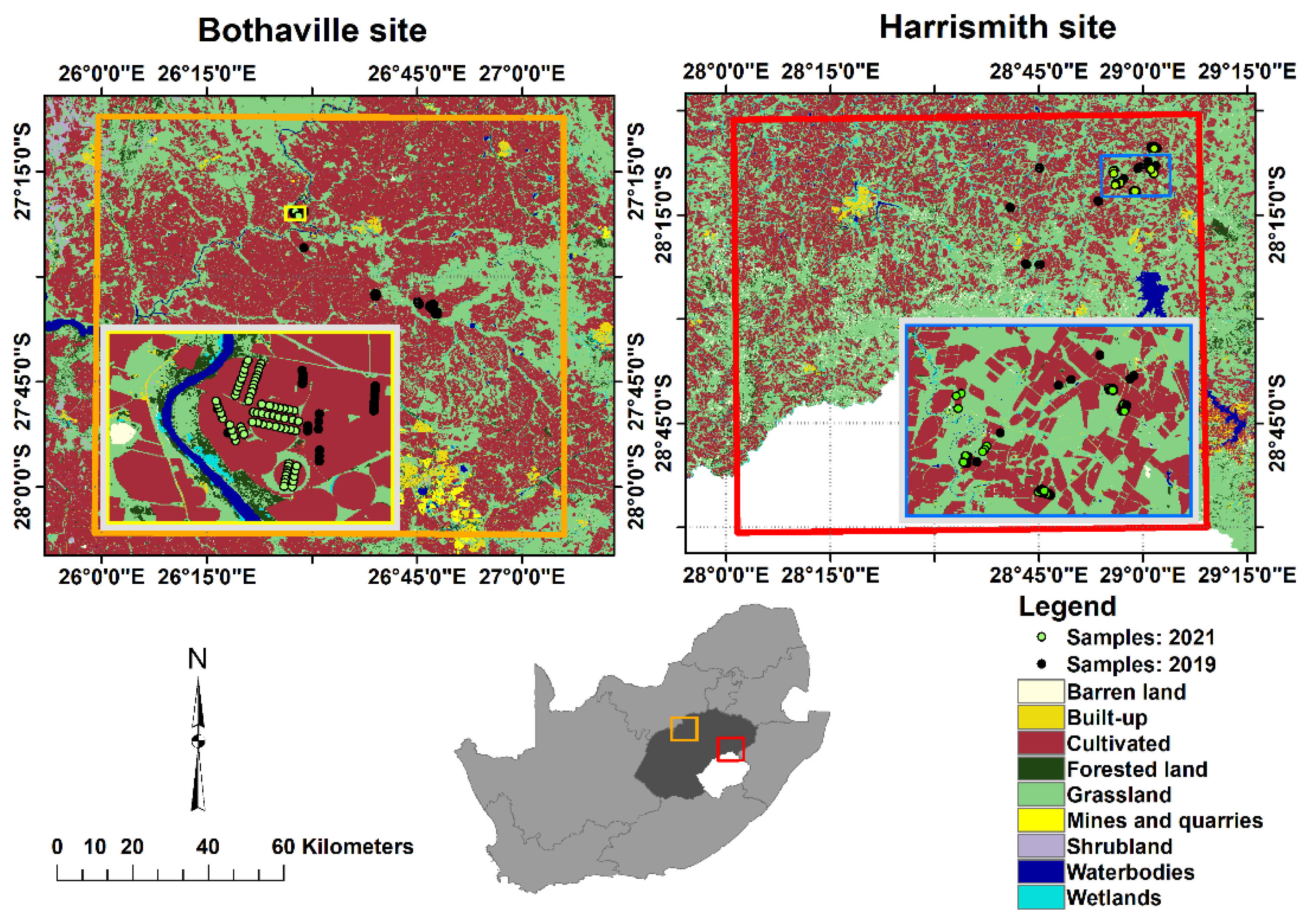
2.1. Characteristics of the Experimental Sites

Two experimental sites, i.e., Bothaville (27°13′0′′S to 28°8′0′′S; 26°0′0′′E to 27°05′0′′E), and Harrismith (28°0′0′′S to 29°0′0′′S; 28°0′0′′E to 29°8′0′′E), located in the Free State province, South Africa were used in this study (Figure 1). The experimental sites, each with 10 000 km² area, are situated in the main agricultural production zone of the country. The two experience wet and warm summers, with mean temperatures of approximately 18 °C and 19.2 °C, and annual mean rainfall of approximately 584 mm and 115 mm, respectively. The summer season represents the main cropping season (i.e., December to May/June), where primarily commercial farming of main crops such as Maize (Zeal mays L.), Soybeans (Glycine max), Dry beans (Phaseolus vulgaris), Sunflower (Helianthus annus L.) and Peanuts (Arachis hypogaea L.) in Bothaville and Maize, Soybeans, Dry beans in Harrismith, occurs. The soil in Bothaville is characterized by sandy-loamy to sandy soils on visibly flat slopes, while Harrismith soil is dominantly clay-loamy with higher water-retention capacities on undulating slopes.

2.2. Data

2.2.1. In-Situ Data

The multi-temporal in-situ LAI and LC_ab data were collected in the two respective experimental sites in 2019 and 2021 at the peak of the season when crops were in their physiological maturity. In Bothaville, the data collection occurred from the 8 to 14 of April and 11 to 23 of April in 2019 and 2021, respectively. In Harrismith, it was collected from the 11 and 15 of March and 15 to 26 of March in 2019 and 2021, respectively. No field campaigns were conducted in 2020 due to the national lockdown imposed to reduce the spread of the COVID-19 pandemic, which coincided with the summer growing season. At each site, LC_ab and LAI measurements were collected from plots of 40 m × 40 m, which were selected along a randomly selected transect. The centroids of each plot were Geo-tagged with a coordinate using a handheld Data Collector (i.e., Trimble^® TDC600), which has a positional accuracy of 1.5 m. LAI measurements were collected with a LiCor 2200c Plant Canopy Analyzer (Li-Cor, Inc., Lincoln, NE, USA) in both field campaigns. To avoid the influence of unequal sky conditions and the operator on the measurements, we used a 180° view cap. In contrast, LC_ab measurements of sun-exposed leaves were taken with Minolta SPAD-502 chlorophyll meter (Minolta, Osaka Co., Ltd., Osaka, Japan) in 2019 and MC-100 Chlorophyll Concentration Meter (Apogee Instruments, Inc., Logan, UT, USA) in 2021, respectively. MC-100 measures chlorophyll content in absolute units, i.e., µmol m⁻², realized through crop-specific and generic calibration coefficients applied to the measured transmission ratio at 931 nm to 653 nm [43]. To be consistent with previous studies, we converted the chlorophyll concentration values from µmol m⁻² to µg cm⁻². In contrast, SPAD-502 provides unitless values (i.e., a relative value proportional to C_ab based on the ratio of transmitted and incident radiation at 940 nm and 650 nm). We used relationships established previously for the same crop types [44,45,46] to convert the SPAD values to LC_ab (µg cm⁻²; Equation (1)).

$${\mathrm{LC}}_{\mathit{a}\mathit{b}}={10}^{SPA{D}^{0.264}-4}\times M,$$

(1)

where SPAD is the value read from SPAD-502Plus and $M$ means the chlorophyll molar mass set at 907 g/mol [47].

For each plot, the canopy chlorophyll content (CCC) was calculated by multiplying LC_ab by LAI (LC_ab × LAI) [48]. Since intercropping and mixed crop management practices dominate African agriculture, our interest was to develop generic BV retrieval models (i.e., with a potential for wide application, especially in semi-arid African contexts). Therefore, the multi-temporal in-situ data for all crops found at both sites, i.e., Maize (Zea mays L.), Soybeans (Glycine max), Dry beans (Phaseolus vulgaris) in Harrismith, and Maize, Soybeans, Dry beans, Sunflower (Helianthus annuus L.) and Peanuts (Arachis hypogaea L.) in Bothaville, were combined and used to extract intersecting surface reflectance values from respective image dates (see Section 2.2.2) within 40 m × 40 m pixel-blocks. Since they have contrasting physiological pathways, leaf and canopy structures and architectures, these crop types represent anatomical and physiological traits of many other crop types [49]. Therefore, we hypothesize that the BV models calibrated using these crops will likely be transferable and widely applicable.

2.2.2. Remotely Sensing Data

Sentinel-2 MSI Analysis-ready-data (ARD, i.e., Level-2A) close to the dates of the fieldwork (see Section 2.2.1) were retrieved from Sentinel Hub (Sinergise Laboratory for geographical information systems, Ltd., Ljubljana, Slovenia) using the Request-Builder for Process API (https://apps.sentinel-hub.com/requests-builder/, accessed on 15 June 2021). The ARD refers to harmonized, standardized, interoperable, and radiometrically and geometrically consistent data that eliminates the pre-processing burden to allow immediate analysis (Dwyer et al., 2018). The retrieved ARD images were acquired on 15 April 2019 (cloud cover: 0.64%) and 14 April 2021 (cloud cover: 0.29%) for Bothaville (35JMK) and 18 March 2019 (cloud cover: 51.47%) and 22 March 2021 (cloud cover: 6.11%) for Harrismith (35JPJ). We used spectral bands centered at 490 nm (B2), 560 nm (B3), 665 nm (B4), and 842 nm (B8) acquired at 10 m resolution, and 705 nm (B5), 740 nm (B6), 783 nm (B7), 865 nm (B8A), 1610 nm (B11), and 2190 nm (B12) at 20 m resolution. To match the resolutions between all bands, we resampled the bands with 10 m resolution to 20 m using the nearest neighbor resampling in SNAP v8.0 (Sentinel Application Platform, http://step.esa.int, accessed on 15 June 2021). Nearest neighbor resampling was chosen due to its ability to retain the spectral fidelity of the data. The systematic ARD data processing is achieved with Sen2Cor by the ESA (European Space Agency) ground segment [50,51,52].

Further analyses were restricted to areas covered by a crop mask which was obtained from the National Crop Boundaries Dataset (CropEstimatesConsortium, 2017), and a vegetation mask created from NDVI was used to mask values < 0.2 following [53].

2.3. eXtreme Gradient Boosting

Extreme Gradient Boosting (XGBoost), proposed by [54], is an improved implementation of Gradient Boosted Regression Trees (GBRT), also known as Gradient Boosting Machines (GBM) [55], bringing several additional features and advantages. Like GBM, the XGBoost is an ensemble of classification and regression trees (CART); where, regression trees are computed sequentially, and new weak learners are included iteratively in the model using additive functions to correct errors from the previous learner. The final model is an ensemble of several weak learners, and final predictions are the sum of the predictions at each iteration. Generally, given the training dataset with predictor and response variables, the XGBoost algorithm first sorts the predictors and searches for the optimal splits. Then, an optimal split is chosen from the predictor that optimizes the objective function, i.e., Squared Error. The above steps are repeated until the most extreme tree depth is achieved. Then, the prediction scores are assigned to the leaves, and any negative nodes are pruned using a bottom-up approach. Until the predetermined number of rounds is reached, the above steps are repeated in a value-adding manner. Mathematical descriptions of XGBoost can be found in [56,57]. The algorithm has several advantages over GBM, which include: (1) it can efficiently handle sparse data or missing values; (2) it uses distributed and parallel computing to construct trees and build large models rapidly; (3) it avoids over-fitting by using a more regularized formalization and gradient boosted decision trees; and (4) the trained model can be used to predict the unseen (i.e., new) data. Thus, XGBoost often outperforms other algorithms, and it is scalable, sparsity-aware, and computationally efficient [54,58]. XGBoost has several hyperparameters which can be tuned. In this study, the hyper-parameters were tuned using the random search strategy [59], over a predefined search space consisting of general, booster-specific and learning task parameters in ‘xgboost’ R package [60]. The optimal hyper-parameters were selected using the lowest Root Mean Squared Error of cross-validation (RMSE_CV) based on the 10-fold Cross Validation (CV) resampling strategy. The open-source XGBoost library for different programming languages and documentation can be found online (https://xgboost.readthedocs.io/en/stable/index.html, accessed on 24 July 2022).

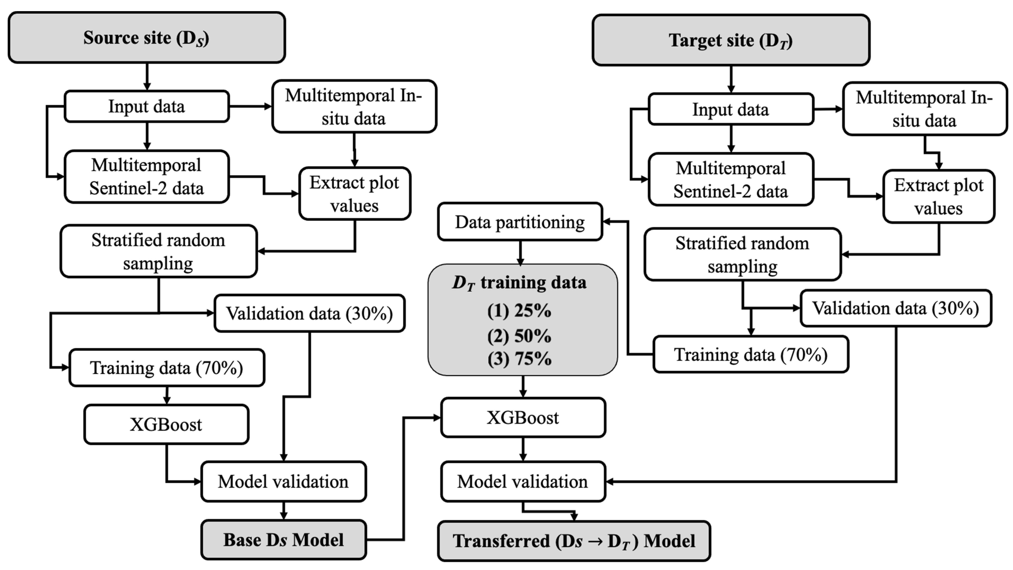
2.4. Spatial Transfer Scenarios

The Source site, i.e., ${\mathcal{D}}_S={\left\{\left({\mathcal{X}}_i^s,{\mathcal{Y}}_i^s\right)\right\}}_{i=1}^{n_s}$, refers to the study site where modelling was performed with all training samples$n_s$, and the Target site ${\mathcal{D}}_T={\left\{\left({\mathcal{X}}_i^l,{\mathcal{Y}}_i^l\right)\right\}}_{i=1}^{n_l}$ is the destination study site where the trained models were transferred with limited training samples $n_l$, where $n_l\ll n_s$. In this regard, three spatial transfer scenarios were assessed, i.e., Base ${\mathcal{D}}_S+25\%$, Base ${\mathcal{D}}_S+50\%$, and Base ${\mathcal{D}}_S+75\%$, where Base ${\mathcal{D}}_S$ is the pre-trained model with multi-temporal data for two spatial transferability cases: Bothaville (${\mathcal{D}}_S$) → Harrismith (${\mathcal{D}}_T$) and Harrismith (${\mathcal{D}}_S$) → Bothaville (${\mathcal{D}}_T$), i.e., when either Bothaville or Harrismith is the Source site. The percentages represent the proportion of available training samples used for re-training the Base ${\mathcal{D}}_S$ model at the Target site ${\mathcal{D}}_T$. For example, trained BV models in the Source site ${\mathcal{D}}_S$ (e.g., Harrismith) were transferred to the Target site ${\mathcal{D}}_T$ (e.g., Bothaville) and vice versa. Alternating the two sites as ${\mathcal{D}}_S$ and ${\mathcal{D}}_T$ provided an opportunity to assess the impact of site characteristics and acquisition conditions on model transferability. The flow chart summarizing the methodology is shown in Figure 2.

2.5. Model Training and Evaluation

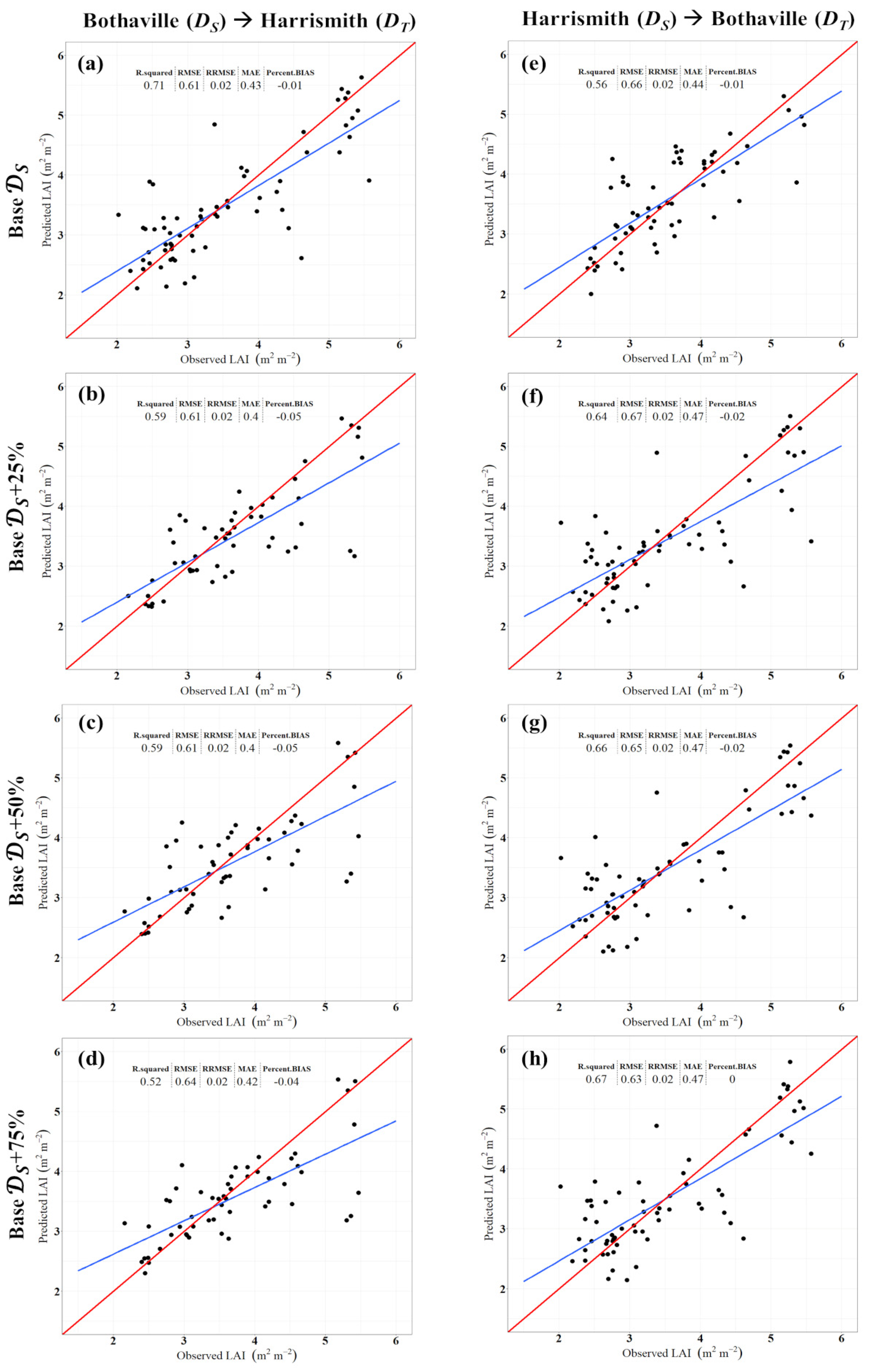
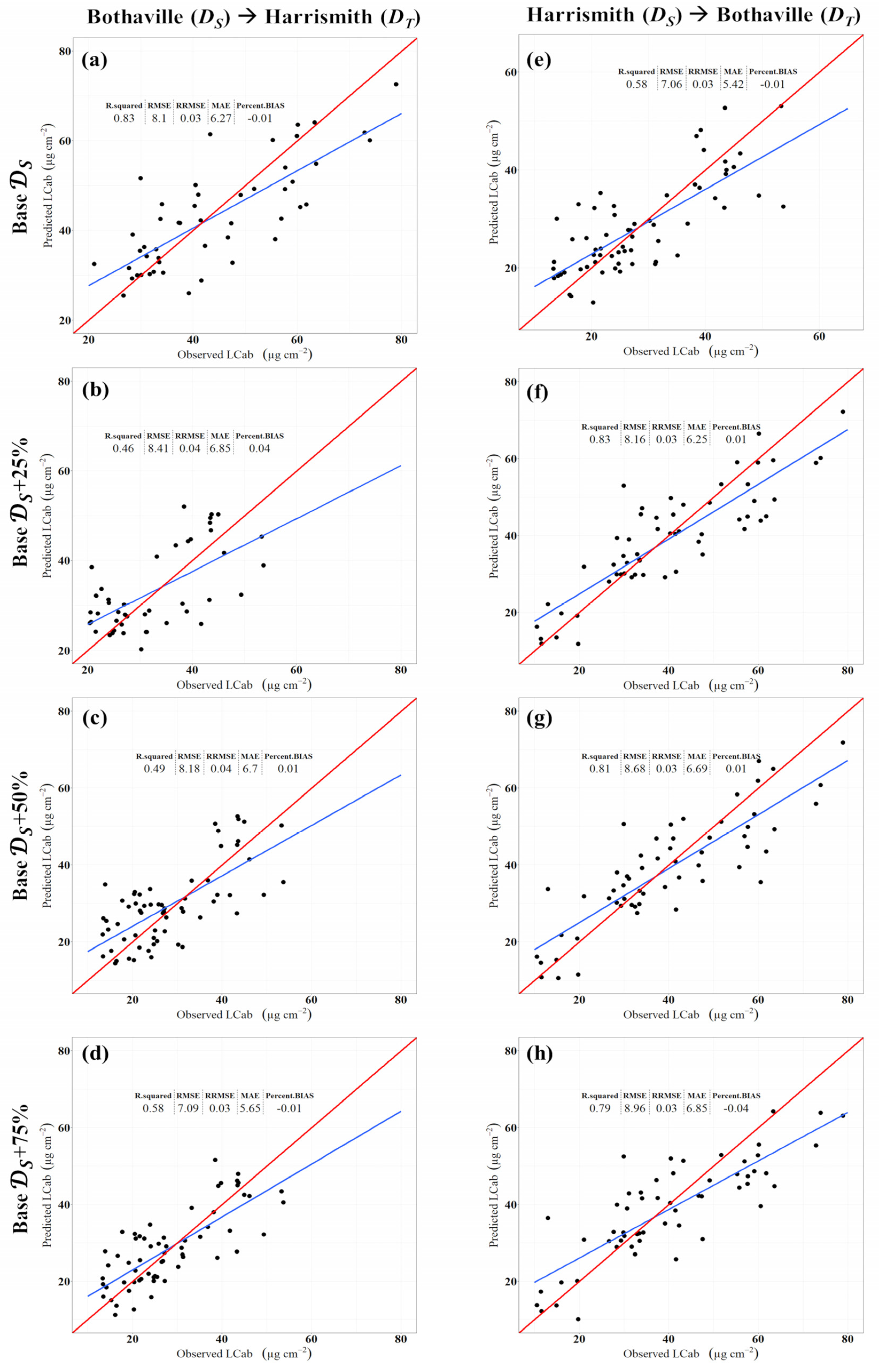
Multi-temporal in-situ data from each respective Source site ${\mathcal{D}}_S$ were used to train and evaluate the transferability of the LAI, LC_ab, and CCC models. Specifically, the Source site ${\mathcal{D}}_S$ data were split into training (i.e., 70%) and validation (i.e., 30%) using a stratified random sampling approach and used for training and validating the Base ${\mathcal{D}}_S$ models, respectively. Then, for re-training transferred models, the Target site ${\mathcal{D}}_T$ training data (i.e., 70%) were randomly split into 25%, 50%, and 75% of samples used in training the Base ${\mathcal{D}}_S$ models (see

Table 1. Descriptive statistics of LAI (m² m⁻²), LCab (µg cm⁻²) and CCC (µg cm⁻²) training samples for Source site (i.e., Base ${\mathcal{D}}_S$) different transfer scenarios, i.e., Base ${\mathcal{D}}_S+25\%$, Base ${\mathcal{D}}_S+50\%$, and Base ${\mathcal{D}}_S+75\%$.

		Bothaville			Harrismith
		LAI	LCab	CCC	LAI	LCab	CCC
Base $𝒟$S	n	166	166	166	147	147	147
	Min	1.54	3.70	11.86	1.16	10.77	20.44
	Mean	3.62	34.53	126.98	3.45	26.83	92.56
	Max	5.90	74.02	288.22	6.32	56.82	333.63
	SD	1.04	15.57	66.99	0.94	10.89	51.25
Base $𝒟$S + 25%	n	202	202	202	188	188	188
	Min	1.54	3.71	11.86	1.16	3.71	11.86
	Mean	3.57	33.07	120.18	3.53	28.35	102.25
	Max	6.35	74.02	288.22	6.32	71.35	333.63
	SD	1.01	15.06	65.33	0.98	12.33	59.63
Base $𝒟$S + 50%	n	239	239	239	229	229	229
	Min	1.54	3.71	11.86	1.16	3.71	11.86
	Mean	3.56	32.04	115.80	3.51	29.97	106.89
	Max	6.35	74.02	288.22	6.32	74.01	333.63
	SD	0.99	14.65	63.66	0.98	13.82	62.47
Base $𝒟$S + 75%	n	276	276	276	270	270	270
	Min	1.54	3.71	11.86	1.16	3.71	11.86
	Mean	3.55	31.36	113.41	3.55	30.58	110.48
	Max	6.35	74.01	333.63	6.32	74.01	333.63
	SD	1.00	14.30	63.31	1.01	14.06	63.15

), and 30% of ${\mathcal{D}}_T$ samples were held-out for evaluating the transferability of the model (i.e., its performance in a new (unseen) site) (see Figure 2). The prediction accuracies of each BV model in the Source and Target sites were assessed with the measures recommended by Richter et al. (2012), i.e., Root Mean Squared Error (RMSE), Coefficient of determination (R²), Relative Root Mean Squared Error (RRMSE), Mean Absolute Error (MAE), and Percent Bias (%Bias) (Equations (2)–(6)). The modelling, validation and mapping were performed using the R-Statistics package: mlr v2.19 (Available online: https://mlr.mlr-org.com/, accessed on 5 March 2022) [61].

$$RMSE=\sqrt{\frac{1}{n} {\displaystyle \sum }_{i=1}^N{(x_{i }\times y_i)}^2}$$

(2)

$$R^2=\frac{{{\displaystyle \sum }}^{}{(y_i^N-{\overline{y}}_i)}^2}{{{\displaystyle \sum }}^{}{(y_i-{\overline{y}}_i)}^2}$$

(3)

$$RRMSE=\frac{RMSE}{{\overline{x}}_i}$$

(4)

$$MAE=\frac{1}{n}{\displaystyle \sum }_{i=1}^n\left|x_i-y_i\right|$$

(5)

$$\%BIAS={{\displaystyle \sum }}_{i=1}^n(x_{i }-y_i)/{{\displaystyle \sum }}_{i=1}^n(x_i),$$

(6)

where x_i is the observed BV (e.g., LAI), and y_i is the predicted biophysical parameter (e.g., LAI), ${\overline{x}}_i$, and ${\overline{y}}_i$ are the mean of observed and predicted BV, respectively; n is the sample size, and N is the number of errors.

3. Results

The evaluation of the spatial transferability of the Machine Learning Regression (MLR) models for estimating crop biophysical and biochemical variables (BVs) is critical for determining their utility in different geographical areas, with a few training samples, different spatial distributions, and spectral shifts due to acquisition conditions and crop types. In this study, we evaluated the spatial transferability of generic BV models based on XGBoost by applying them to different target experimental sites, under different transfer scenarios, designed based on the proportion of the training data available in the Target sites, i.e., 25%, 50%, and 75%. Specifically, we applied pre-trained Source site models (from Bothaville and Harrismith), i.e., Base ${\mathcal{D}}_S$, to Target sites (i.e., Harrismith and Bothaville) with 25%, 50%, and 75% available, randomly selected training samples, yielding BV models with Base ${\mathcal{D}}_S+25\%$, Base ${\mathcal{D}}_S+50\%$, and Base ${\mathcal{D}}_S+75\%$. The performances of the Base ${\mathcal{D}}_S$ and transferred models to different Target sites ${\mathcal{D}}_T$ (i.e., Bothaville and Harrismith) are presented in Figure 3, Figure 4 and Figure 5 for LAI, LC_ab, and CCC, respectively. As shown in Figure 3a,e, Bothaville Base ${\mathcal{D}}_S$ LAI model had better performance (i.e., RMSE: 0.61 m² m⁻², R²: 0.71) than the Harrismith Base ${\mathcal{D}}_S$ LAI model (i.e., RMSE: 0.66 m² m⁻², R²: 56). The Bothaville Base ${\mathcal{D}}_S$ LAI models with 25% (i.e., Base ${\mathcal{D}}_S+25\%$) and 50% (i.e., Base ${\mathcal{D}}_S+50\%$) training samples in the Target site ${\mathcal{D}}_T$ (i.e., Harrismith) have a better RMSE of 0.61 m² m⁻² (R: 0.59) compared to the Harrismith Base ${\mathcal{D}}_S$ LAI model, but exhibited relatively higher underestimations, i.e., percent bias of 5% (see Figure 3b,c). In contrast, when the Bothaville Base ${\mathcal{D}}_S$ LAI model was re-trained with 75% of the samples in the ${\mathcal{D}}_T$ (i.e, Harrismith, Figure 3d), the results maintained a better RMSE of 0.64 m² m⁻² when compared to the Harrismith Base ${\mathcal{D}}_S$ LAI model (i.e., RMSE: 0.66 m² m⁻²), but the differences were not significant. Moreover, the transferred model explained only 52% of LAI variability in the Target site ${\mathcal{D}}_T$ (i.e., Harrismith).

When considering Harrismith as the Source site ${\mathcal{D}}_S$ and Bothaville as the Target site ${\mathcal{D}}_T$, the results using Base ${\mathcal{D}}_S+25\%$ LAI model (Figure 3f) showed an inferior RMSE of 0.67 m² m⁻² relative to the Bothaville Base ${\mathcal{D}}_S$ LAI model, i.e., RMSE:0.61 m² m⁻² (Figure 3a). Similarly, the transferred model (Base ${\mathcal{D}}_S+25\%$) explained relatively lower LAI variability in the Target site ${\mathcal{D}}_T$ (Figure 3f), i.e., 64%, and marginally high underestimations, i.e., by 1%. The higher proportions of training samples in ${\mathcal{D}}_T$ (i.e, Bothaville) seems to have benefited model accuracy, with Base ${\mathcal{D}}_S+50\%$ (Figure 3g) and Base ${\mathcal{D}}_S+75\%$ (Figure 3h) achieving relatively better RMSEs of 0.65 m² m⁻² and 0.63 m² m⁻², respectively, and explaining higher LAI variability, i.e., 66% and 67%, respectively, when compared to Base ${\mathcal{D}}_S+25\%$ model (Figure 3f). While underestimations for Base ${\mathcal{D}}_S+50\%$ (Figure 3g) were similar to Base ${\mathcal{D}}_S+25\%$ (i.e., %Bias: 2%, Figure 3f), a 0% percent bias was found for Base ${\mathcal{D}}_S+75\%$ (Figure 3h).

Leaf Chlorophyll Content (LC_ab) Base ${\mathcal{D}}_S$ models in Bothaville and Harrismith also had different performances. The Bothaville Base ${\mathcal{D}}_S$ LC_ab model (Figure 4a) explained the greatest variability, i.e., 83% compared to only 58% achieved by the Harrismith Base ${\mathcal{D}}_S$ LC_ab model (Figure 4e). However, the RMSE of the Bothaville Base ${\mathcal{D}}_S$ LC_ab model was higher, i.e., 8.1 µg cm⁻², than that of Harrismith Base ${\mathcal{D}}_S$ LC_ab model, which achieved a relatively lower RMSE of 7.06 µg cm⁻². When the Bothaville Base ${\mathcal{D}}_S$ LC_ab model was transferred to Harrismith (i.e., Bothaville (${\mathcal{D}}_S$) → Harrismith (${\mathcal{D}}_T$)) with 25% training samples in ${\mathcal{D}}_T$(i.e., Base ${\mathcal{D}}_S+25\%$), the results (Figure 4b) indicate an RMSE, i.e., 8.41 µg cm⁻² and explained 46% of LC_ab variability in Harrismith. The Base ${\mathcal{D}}_S+25\%$ also led to an overestimation of 4% when compared to validation data. When the proportion of training samples in the Target site ${\mathcal{D}}_T$ (i.e., Harrismith) were increased to 50%, i.e., Base ${\mathcal{D}}_S+50\%$ (Figure 4c), the RMSE and R² improved slightly to 8.18 and 0.49, respectively. Similarly, an increase in the Target site ${\mathcal{D}}_T$ samples to 75%, i.e., Base ${\mathcal{D}}_S+75\%$ (Figure 4d), improved the RMSE to 7.09 (i.e., equivalent to the one achieved by the fully trained model) and 58% of LC_ab variability was explained in the Target site ${\mathcal{D}}_T$ (i.e., Harrismith).

In contrast, the Harrismith Base ${\mathcal{D}}_S$ LC_ab model transferred to Bothaville (i.e., Harrismith (${\mathcal{D}}_S$) → Bothaville (${\mathcal{D}}_T$)) showed improvements in RMSE, even with the smallest proportion of samples, i.e., 25%, in ${\mathcal{D}}_T$(Base ${\mathcal{D}}_S+25\%$), explaining 83% of LC_ab variability in ${\mathcal{D}}_T$ (i.e., Bothaville) and RMSE of 8.16 µg cm⁻² (Figure 4f), which was equivalent to the Bothaville Base ${\mathcal{D}}_S$ LC_ab model (Figure 4a). The addition of 50% (Figure 4g) and 75% (Figure 4h) of ${\mathcal{D}}_T$ (i.e., Bothaville) training samples resulted in relatively worse LC_ab retrievals, with the former (i.e., Base ${\mathcal{D}}_S+50\%$) yielding RMSE of 8.68 µg cm⁻² and R² of 0.81 (Figure 4g), while the latter (i.e., Base ${\mathcal{D}}_S+75\%$) achieving inferior RMSE of 8.96 µg cm⁻², R² of 0.79 and higher underestimations of 4%. Nonetheless, all the transferred models had RRMSE of <5% in both cases, i.e., Bothaville (${\mathcal{D}}_S$) → Harrismith (${\mathcal{D}}_T$) and Harrismith (${\mathcal{D}}_S$) → Bothaville (${\mathcal{D}}_T$).

The Bothaville Base ${\mathcal{D}}_S$ CCC model had better RMSE, i.e., 37.12 µg cm⁻², and explained greater variability, i.e., 79%, (Figure 5a) than the Harrismith Base ${\mathcal{D}}_S$ CCC model, which achieved RMSE of 38.57 µg cm⁻² and R² of 0.56 (Figure 5e). Similar to LC_ab models, Bothaville CCC models, i.e., Bothaville (${\mathcal{D}}_S$) → Harrismith (${\mathcal{D}}_T$), resulted in poor retrieval when only 25% of ${\mathcal{D}}_T$ samples were used, i.e., RMSE: 40.43 µg cm⁻², R²: 0.52 (see Figure 5b). While proportions, i.e., 50% (i.e., Base ${\mathcal{D}}_S+50\%$) and 75% (i.e., Base ${\mathcal{D}}_S+75\%$), led to better retrieval accuracies, i.e., RMSE: 40.18 µg cm⁻² (Figure 5c) and 36.3 µg cm⁻² (Figure 5d), respectively. The Base ${\mathcal{D}}_S+50\%$ model explained 52% of CCC variability in the Target site ${\mathcal{D}}_T$ (i.e., Harrismith), while Base ${\mathcal{D}}_S+75\%$ explained 61% of CCC variability. Moreover, the ${\mathcal{D}}_S+25\%$ model also had higher underestimations of CCC, i.e., %Bias of 4%, than other transferred models, which had a %Bias of only 1%. The Harrismith (${\mathcal{D}}_S$) → Bothaville (${\mathcal{D}}_T$) model, re-trained with 25% of the samples in the Target site ${\mathcal{D}}_T$ (i.e., Bothaville) (Figure 5f), showed better CCC retrieval accuracy, i.e., RMSE: 40.25 µg cm⁻², R²: 0.77, than other transfer scenarios, i.e., Base ${\mathcal{D}}_S+50\%$ (RMSE: 41.39 µg cm⁻², R²: 0.76) and Base ${\mathcal{D}}_S+75\%$ (RMSE: 42 µg cm⁻², R²: 0.74). The Base ${\mathcal{D}}_S+25\%$ model (Figure 5f) and Base ${\mathcal{D}}_S+75\%$ model (Figure 5h) had underestimations of 3%, while the Base ${\mathcal{D}}_S+50\%$ had a %Bias of 0%. All the transferred models were significant (p < 2.2 × 10⁻¹⁶).

The spatial distribution maps of biophysical and biochemical variables retrieved with Source (i.e., Base ${\mathcal{D}}_S$) and best transferred models (${\mathcal{D}}_T$) are presented in Figure 6 and Figure 7. Figure 6 shows Bothaville (${\mathcal{D}}_S$) and Harrismith (${\mathcal{D}}_S$) → Bothaville (${\mathcal{D}}_T$) transferred retrievals ((d)–(e)), while Figure 7 shows Harrismith (${\mathcal{D}}_S$, (a)–(c)) and Bothaville (${\mathcal{D}}_S$) → Harrismith (${\mathcal{D}}_T$) transferred retrievals ((d)–(e)). As shown, the retrievals from transferred models show underestimations of all BVs in Bothaville when compared to the Source site (i.e., Base ${\mathcal{D}}_S$) spatial distribution maps. On the other hand, Bothaville (${\mathcal{D}}_S$) → Harrismith (${\mathcal{D}}_T$) maps (Figure 7) show relatively similar spatial distributions for all BVs.

4. Discussions

The transferability of retrieval approaches has been a major challenge yet critical for reducing the need for large training sets, reducing computational costs associated with calibrating MLRAs and improving the operational access to important crop BVs in data-scarce areas. For this study, we considered a case of spatial transferability technique, where a trained Source model (i.e., Base ${\mathcal{D}}_S$) is transferred to a new site (i.e., Target site ${\mathcal{D}}_T$) with different proportions of training samples available (relative to the ones used in the Base ${\mathcal{D}}_S$) for re-training the transferred model. Then, the transferred models’ performance was compared against the fully trained model in the Target site ${\mathcal{D}}_T$ to determine the optimal proportion of samples that delivers comparable results. Moreover, the effect of the Source site model (i.e., Base ${\mathcal{D}}_S$) accuracy on its transferability was evaluated.

4.1. Effect of Training Samples Available in the Target Site

The assessment of the impact of the available training samples on the Target site ${\mathcal{D}}_T$ on the transferability of the MLRA biophysical variables (BVs) retrieval models is significant for determining the optimal proportion of training samples required for successfully transferring models to new (unseen) areas, critical for operational agronomic applications. Generally, the results showed that Bothaville (${\mathcal{D}}_S$) → Harrismith (${\mathcal{D}}_T$) models required only fewer proportions, i.e., 25% or 50%, of the training samples to make reliable retrievals of LAI in the Target site ${\mathcal{D}}_T$ (Harrismith). However, this was not true for Harrismith (${\mathcal{D}}_S$) → Bothaville (${\mathcal{D}}_T$) models, where the results show that the transferred models with higher proportions of training samples, i.e., 75%, were more accurate (see Figure 3h). This observation implies that the proportion of samples required to make reliable LAI retrievals depends on the characteristics of the Source site ${\mathcal{D}}_S$. For example, the crop types varied between Bothaville and Harrismith, where the former is characterized by Maize, Peanuts, Sunflower, and Beans, while Harrismith was mainly dominated by Maize and Beans. Therefore, Bothaville (${\mathcal{D}}_S$) → Harrismith (${\mathcal{D}}_T$) models explained the variability caused by different crop types in the Target site ${\mathcal{D}}_T$ (i.e., Harrismith) relatively well, while Harrismith (${\mathcal{D}}_S$) → Bothaville (${\mathcal{D}}_T$) models required a considerable amount of samples (i.e., up to 75%) to learn new (i.e., unseen) distributions caused by the new crop types (i.e., Peanuts and Sunflower) with distinct structural characteristics which were encountered in the Target site ${\mathcal{D}}_T$ (i.e., Bothaville). Besides the different crop types, the different edaphic factors such as soil types (sandy-loamy soils vs. clay-loamy) and soil moisture between sites—known to affect surface reflectance and LAI variability (Darvishzadeh et al., 2008)—may have contributed to the requirement for a large proportion of samples to improve transferability of the Harrismith (${\mathcal{D}}_S$) → Bothaville (${\mathcal{D}}_T$) LAI model. Although cropping at the two sites occurs within the same crop calendar and in-situ measurements were collected when plants were in their physiological maturity, it is anticipated that there were some spectral shifts caused browning of some leaves in the canopies which may have been pronounced in Bothaville (fieldwork in April) than in Harrismith (fieldwork in March). Without the additional samples, the model resulted in relatively higher errors (see Figure 3f,g). However, the improvements brought by increasing the ${\mathcal{D}}_T$ training samples in the case of Harrismith (${\mathcal{D}}_S$) → Bothaville (${\mathcal{D}}_T$) were incremental but marginal, thus signaling that the contrasting canopy architectures of Maize and Beans found in Harrismith played a key role in the model transferability but were not sufficiently representative to explain variability caused by other crop types present in the ${\mathcal{D}}_T$ (i.e., Bothaville). Nonetheless, the transferred LAI model achieved comparable accuracies (RMSE: 0.63 m² m⁻²; R²: 0.61) to a Gradient Boosting Machine model in a related previous study over ${\mathcal{D}}_T$ [62]. Moreover, all the transferred LAI models performed better than the artificial neural networks pre-trained with PROSAIL-simulated look-up tables (LUTs) which achieved RMSE >1 m² m^–2 in Bothaville [63] and elsewhere [64,65].

For chlorophyll content models (Figure 4 and Figure 5), the Bothaville (${\mathcal{D}}_S$) → Harrismith (${\mathcal{D}}_T$) models required a significant proportion of ${\mathcal{D}}_T$ training samples to achieve a comparable retrieval accuracy to the model trained with all the training samples in Harrismith. In contrast, the Base ${\mathcal{D}}_S$ model experienced significant accuracy losses when transferred and re-trained with 25% (i.e., Base ${\mathcal{D}}_S+25\%$) and 50% (Base ${\mathcal{D}}_S+50\%$). This implies that the smaller training samples (i.e., 25% and 50%) were insignificant to account for the variability in the Target site ${\mathcal{D}}_T$ (i.e., Harrismith), which was probably caused by the different crop growth stages and plant structural forms present at the two experimental sites. In the case of Harrismith (${\mathcal{D}}_S$) → Bothaville (${\mathcal{D}}_T$), the lower proportion of ${\mathcal{D}}_T$ training samples (i.e., 25%) were sufficient to achieve the optimal retrieval accuracies while increasing the proportion of samples caused a decline. Generally, the results showed that the XGBoost models could be transferred to different areas with various crop types and crop phenology with minimal losses to the retrieval accuracies; however, the number of samples required for re-training the source models depended on the BV and the Source site ${\mathcal{D}}_S$ characteristics. The RRMSEs for all the transferred BV models under all spatial transfer scenarios were 5% and below, hence below the recommended limits by the Global Climate Observing System (GCOS) [66].

4.2. Source Model Accuracy and Its Effect on Transferred XGBoost Models

It is crucial to understand the effect of the source model accuracy on its transferability. Here, we evaluate the magnitude of this effect, if any, under the different transfer scenarios. The results indicated that the accuracy of the source model (i.e., Base ${\mathcal{D}}_S$) is important to ensure lower accuracy losses when the model is transferred to an unseen (i.e., new) site. For example, when Bothaville Base ${\mathcal{D}}_S$ LAI model (with RMSE: 0.61 m² m⁻²; R²: 0.71) was transferred to Harrismith (i.e., Bothaville (${\mathcal{D}}_S$) → Harrismith (${\mathcal{D}}_T$)), only a few training samples (i.e., 25%) were required in the Target site ${\mathcal{D}}_T$ to obtain improved RMSE and R² by 0.05 m² m⁻² and 3%, respectively, relative to the fully trained model in Harrismith (Figure 3b,e). Conversely, in the case of Harrismith (${\mathcal{D}}_S$) → Bothaville (${\mathcal{D}}_T$), the Harrismith Base ${\mathcal{D}}_S$ LAI model—with RMSE of 0.66 m² m⁻² and R² of 0.56—required a significant proportion of training samples (i.e., 75%) to achieve better accuracy, which remained lower than the fully trained model in the Source site ${\mathcal{D}}_S$ (Figure 3a,h). Therefore, when the Source model is highly accurate, its likelihood to perform better in the Target site (with few additional samples) increases. Essentially, the higher the variability explained by the source model, the lower the proportion of samples needed to account for the new variability in the target site.

The chlorophyll content is a highly dynamic BV due to its sensitivity to various biotic (such as pests and diseases) and abiotic factors (such as water, temperature, and nutrients), hence may vary significantly within and between fields containing similar or different crop types relative to LAI, which may remain the same despite the minor changes in chlorophyll content. Interestingly, the lower variability explained by the Harrismith Base ${\mathcal{D}}_S$ LC_ab and CCC models (Figure 4e) did not negatively impact the transferred models’ performance and required only a few training samples (i.e., 25%) to explain the LC_ab and CCC variabilities in the Target site ${\mathcal{D}}_T$ (i.e., Bothaville) (Figure 4f and Figure 5f), and the accuracies were comparable to the fully trained models (Figure 4a and Figure 5a). While the Bothaville Base ${\mathcal{D}}_S$ LC_ab and CCC models (Figure 4a and Figure 5a) explained 83% and 79% of LC_ab and CCC variability, respectively, they suffered accuracy losses when transferred to the Target site ${\mathcal{D}}_T$ (i.e., Harrismith), particularly when only 25% and 50% of ${\mathcal{D}}_T$ training samples were used (Figure 4b,c and Figure 5b,c). As a result, a high proportion of samples, i.e., 75%, were required to achieve comparable or better accuracies to the respective fully trained models in Harrismith (Figure 4e and Figure 5e). These findings may be attributed to the differences in the ranges of LC_ab values; where, in the case of Bothaville (${\mathcal{D}}_S$) → Harrismith (${\mathcal{D}}_T$), the source model could not explain unseen LC_ab values below 20 µg cm⁻² which were evidently present in the Target site ${\mathcal{D}}_T$ (i.e., Harrismith) but not learned by the Base ${\mathcal{D}}_S$ model. Whereas the Base ${\mathcal{D}}_S$ CCC model had a relatively greater range, the values encountered when transferring the model could not be well interpolated using fewer training samples, i.e., 25% and 50%. Hence, for both BVs, the source models required a significant amount of training data to achieve comparable accuracies to the fully trained model in the Target site ${\mathcal{D}}_T$ (i.e., Harrismith). On the other hand, despite a relatively lower LC_ab range in the case of Harrismith (${\mathcal{D}}_S$) → Bothaville (${\mathcal{D}}_T$), the values above 50 µg cm⁻² were a few and well accounted for when the model was transferred and re-trained with 25% of the ${\mathcal{D}}_T$ training samples. Moreover, the overestimations of values ~20 µg cm⁻² observed in the scatterplot of the source model from Harrismith (see Figure 5e) seem to have benefitted the performance of the transferred model since these overestimations were well within the range in the Target site ${\mathcal{D}}_T$ (Bothaville). Because the source model contained values below ~20 µg cm⁻² (i.e., not measured in the ${\mathcal{D}}_T$), the transferred model increased the range of LC_ab retrievals, which was beneficial to the transferred model. Similarly, the saturation of the Base ${\mathcal{D}}_S$ CCC model in Harrismith at ~200 µg cm⁻² was averted by the additional re-training with 25% of the Target site ${\mathcal{D}}_T$ training samples and benefited the retrieved CCC range. Overall, the results indicate that the source model (i.e., Base ${\mathcal{D}}_S$) accuracy is important for BVs that do not vary much at a specific crop phenological stage such as LAI at physiological maturity, while for rapidly changing BVs such as LC_ab and CCC, the source model (i.e., Base ${\mathcal{D}}_S$) accuracy could be averted by re-training with some proportion of training samples. However, in both ${\mathcal{D}}_S$ and ${\mathcal{D}}_T$, the range of BV values played a significant role, where ranges are a different significant number of training samples, i.e., 75%, were required.

4.3. Sources of Uncertainty

Despite the promising results, there were several potential sources of uncertainty. The degree of uncertainty observed when the LC_ab and CCC models were transferred can be attributed to the use of different chlorophyll instruments, i.e., Minolta SPAD-502 chlorophyll meter and MC-100 Chlorophyll Concentration Meter, between the two periods, i.e., 2019 and 2021, respectively. While MC-100 measures the absolute chlorophyll values, the SPAD-502 chlorophyll meter measures an index related to LC_ab and requires site-specific calibration using destructive and lab-measured chlorophyll content for different crop types and leaf structural types. In our study, empirical calibration equations developed elsewhere were used instead due to a lack of laboratory calibration data. Unfortunately, such calibration equations may yield inconsistent results since the SPAD values saturate at LC_ab > 40 µg cm⁻² and vary by species, growth stages and distribution of LC_ab [45,67,68]. Future studies should consider cross-calibration of the two instruments and attempt a systematic error adjustment of the field measurements taken by the two instruments. This may lead to improved accuracy of the transferred model and the replicability of the results. Moreover, the edaphic factors at each site such as soil types and moisture, as well as other site characteristics such as differences in planting dates and thus crop phenology within and between fields, may have affected the measured crop biophysical parameters, presenting varying BV values to XGBoost per site. One of the known limitations of MLRAs is that they are not capable of estimating beyond the input values used during training; therefore, sufficient data covering multiple years, crop phenology and areas are needed to further calibrate the models. However, there is generally a lack of consistent and dedicated field campaigns in semi-arid areas of sub-Saharan Africa, thus hindering the development of crop biophysical variables (BVs) and the adoption of precision farming. Nonetheless, the results obtained in this study demonstrate that the XGBoost models can be spatially transferable under the assessed scenarios and are better than those obtained by [42] who found RMSEs between 0.7 m² m⁻² and 0.9 m² m⁻² when Support Vector Machine and Random Forest LAI models were transferred. For all the BVs, the image quality, particularly caused by different atmospheric conditions between the acquisition dates, has affected the source model (Base ${\mathcal{D}}_S$) accuracies and their spatial transferability. For example, ${\mathcal{D}}_S$ and ${\mathcal{D}}_T$ acquisition conditions were different, i.e., >50% clouds in Harrismith for the 2019 image, which propagated to the BV models and hindered the accuracy of Harrismith source models and hence their transferability. Although Sen2cor is the Sentinel-2-specific atmospheric correction technique, its performance has been questionable. The validation and inter-comparison studies [69,70,71,72] show that it performs inconsistently for different spectral bands, land cover types and environments. For the 2019 image over Harrismith used here, [70] showed that under such partly-cloud conditions, Sen2Cor performed poorly, i.e., R² < 20%, in the visible (VIS) and SWIR bands when validated against field data, while it had better performance, i.e., R² > 60%, in the red-edge and NIR bands. Previous studies show that both VIS and SWIR bands are highly influential in LAI, LC_ab and CCC retrieval [62,73,74]. Therefore, the observed lack of transferability with only 25% of samples for Harrismith (${\mathcal{D}}_S$) → Bothaville (${\mathcal{D}}_T$) LAI models and Bothaville (${\mathcal{D}}_S$) → Harrismith (${\mathcal{D}}_T$) LC_ab and CCC models could be due to the residual errors after Sen2Cor atmospheric correction and lower sunlit intensity [29]. In future, predictors should be optimized for various crop BVs according to their relative influence and quality as it has been recently shown that fewer input predictors improve spatial transferability in classification problems [75].

5. Conclusions

Evaluating model transferability is critical for determining the utility of the model in different geographical areas, with a few training samples, different geographical distributions, and spectral shifts due to acquisition conditions and crop types. In this study, we evaluated the spatial transferability of the XGBoost BV models by applying them to different experimental sites under different spatial transfer scenarios, i.e., when 25%, 50%, and 75% of samples are available in the new (unseen) site. Consequently, the effect of different proportions of available training samples in the Target site ${\mathcal{D}}_T$ (i.e., 25%, 50%, and 75%) were assessed, where the ${\mathcal{D}}_T$ consisted of the two semi-arid experimental sites, i.e., Bothaville and Harrismith. Moreover, the effect of the Source site ${\mathcal{D}}_S$ (trained) model accuracy on the Target site ${\mathcal{D}}_T$ (unseen) model uncertainty was also evaluated. The results showed some dependence on the Source site ${\mathcal{D}}_S$ characteristics such as crop types and plant structural characteristics for LAI retrievals, where models from Bothaville—trained with a variety of crop types—could be transferred with only a few samples, i.e., 25%, required in the ${\mathcal{D}}_T$ for obtaining reliable LAI retrievals. On the contrary, the Source site ${\mathcal{D}}_S$ LAI models from Harrismith required significantly higher proportions of training samples in the ${\mathcal{D}}_T$ to obtain reliable retrievals. When it comes to chlorophyll content at both leaf and canopy levels, i.e., LC_ab and CCC, respectively, the factors determining transferability can be attributed to its highly dynamic nature, variability within and between fields and crop types, and due to different field instruments used between the years, i.e., SPAD vs. MC-100. However, it was established that the data range of the trained source models matters, where the unseen low or high BV ranges may deter the transferability of the model. Moreover, the Source site model accuracy has a lesser role when the trained and unseen data ranges differ. The results obtained in this study are better than those in previous related studies, thus demonstrating prospects for achieving reliable retrievals of essential crop BV without requiring many additional samples in the target sites.

References

1. Stamatiadis, S.; Schepers, J.S.; Evangelou, E.; Glampedakis, A.; Glampedakis, M.; Dercas, N.; Tsadilas, C.; Tserlikakis, N.; Tsadila, E. Variable-Rate Application of High Spatial Resolution Can Improve Cotton N-Use Efficiency and Profitability. Precis. Agric. 2020, 21, 695–712. [Google Scholar] [CrossRef]
2. Maine, N.; Lowenberg-DeBoer, J.; Nell, W.T.; Alemu, Z.G. Impact of Variable-Rate Application of Nitrogen on Yield and Profit: A Case Study from South Africa. Precis. Agric. 2010, 11, 448–463. [Google Scholar] [CrossRef]
3. Boyer, C.N.; Wade Brorsen, B.; Solie, J.B.; Raun, W.R. Profitability of Variable Rate Nitrogen Application in Wheat Production. Precis. Agric. 2011, 12, 473–487. [Google Scholar] [CrossRef]
4. Monaghan, J.M.; Daccache, A.; Vickers, L.H.; Hess, T.M.; Weatherhead, E.K.; Grove, I.G.; Knox, J.W. More “Crop per Drop”: Constraints and Opportunities for Precision Irrigation in European Agriculture. J. Sci. Food Agric. 2013, 93, 977–980. [Google Scholar] [CrossRef]
5. Chen, S.; Wang, S.; Shukla, M.K.; Wu, D.; Guo, X.; Li, D.; Du, T. Delineation of Management Zones and Optimization of Irrigation Scheduling to Improve Irrigation Water Productivity and Revenue in a Farmland of Northwest China. Precis. Agric. 2020, 21, 655–677. [Google Scholar] [CrossRef]
6. Meron, M.; Tsipris, J.; Orlov, V.; Alchanatis, V.; Cohen, Y. Crop Water Stress Mapping for Site-Specific Irrigation by Thermal Imagery and Artificial Reference Surfaces. Precis. Agric. 2010, 11, 148–162. [Google Scholar] [CrossRef]
7. Campos-Taberner, M.; Moreno-Martínez, Á.; García-Haro, F.J.; Camps-Valls, G.; Robinson, N.P.; Kattge, J.; Running, S.W. Global Estimation of Biophysical Variables from Google Earth Engine Platform. Remote Sens. 2018, 10, 1167. [Google Scholar] [CrossRef]
8. Dimitrov, P.; Kamenova, I.; Roumenina, E.; Filchev, L.; Ilieva, I.; Jelev, G.; Gikov, A.; Banov, M.; Krasteva, V.; Kolchakov, V.; et al. Estimation of Biophysical and Biochemical Variables of Winter Wheat through Sentinel-2 Vegetation Indices. Bulg. J. Agric. Sci. 2019, 25, 819–832. [Google Scholar]
9. Gitelson, A.A.; Peng, Y.; Huemmrich, K.F. Relationship between Fraction of Radiation Absorbed by Photosynthesizing Maize and Soybean Canopies and NDVI from Remotely Sensed Data Taken at Close Range and from MODIS 250 m Resolution Data. Remote Sens. Environ. 2014, 147, 108–120. [Google Scholar] [CrossRef]
10. Wilhelm, W.W.; Ruwe, K.; Schlemmer, M.R. Comparison of Three Leaf Area Index Meters in a Corn Canopy. Crop Sci. 2000, 40, 1179–1183. [Google Scholar] [CrossRef]
11. Bréda, N.J.J. Ground-Based Measurements of Leaf Area Index: A Review of Methods, Instruments and Current Controversies. J. Exp. Bot. 2003, 54, 2403–2417. [Google Scholar] [CrossRef] [PubMed]
12. Myneni, R.B.; Hoffman, S.; Knyazikhin, Y.; Privette, J.L.; Glassy, J.; Tian, Y.; Wang, Y.; Song, X.; Zhang, Y.; Smith, G.R.; et al. Global Products of Vegetation Leaf Area and Fraction Absorbed PAR from Year One of MODIS Data. Remote Sens. Environ. 2002, 83, 214–231. [Google Scholar] [CrossRef]
13. García-Haro, F.J.; Campos-Taberner, M.; Muñoz-Marí, J.; Laparra, V.; Camacho, F.; Sánchez-Zapero, J.; Camps-Valls, G. Derivation of Global Vegetation Biophysical Parameters from EUMETSAT Polar System. ISPRS J. Photogramm. Remote Sens. 2018, 139, 57–74. [Google Scholar] [CrossRef]
14. Baret, F.; Weiss, M.; Verger, A.; Smets, B. ATBD for LAI, FAPAR and FCOVER from PROBA-V Products at 300 m Resolution (GEOV3); INRA: Paris, France, 2013; Volume 61. [Google Scholar]
15. Gitelson, A.A.; Gritz, Y.; Merzlyak, M.N. Relationships between Leaf Chlorophyll Content and Spectral Reflectance and Algorithms for Non-Destructive Chlorophyll Assessment in Higher Plant Leaves. J. Plant Physiol. 2003, 160, 271–282. [Google Scholar] [CrossRef] [PubMed]
16. Huete, A.; Didan, K.; Miura, T.; Rodriguez, E.P.; Gao, X.; Ferreira, L.G. Overview of the Radiometric and Biophysical Performance of the MODIS Vegetation Indices. Remote Sens. Environ. 2002, 83, 195–213. [Google Scholar] [CrossRef]
17. Mutanga, O.; Skidmore, A.K. Narrow Band Vegetation Indices Overcome the Saturation Problem in Biomass Estimation. Int. J. Remote Sens. 2004, 25, 3999–4014. [Google Scholar] [CrossRef]
18. Jiang, Z.; Huete, A.; Didan, K.; Miura, T. Development of a Two-Band Enhanced Vegetation Index without a Blue Band. Remote Sens. Environ. 2008, 112, 3833–3845. [Google Scholar] [CrossRef]
19. Fitzgerald, G.; Rodriguez, D.; O’Leary, G. Measuring and Predicting Canopy Nitrogen Nutrition in Wheat Using a Spectral Index-The Canopy Chlorophyll Content Index (CCCI). Field Crops Res. 2010, 116, 318–324. [Google Scholar] [CrossRef]
20. Delegido, J.; Verrelst, J.; Meza, C.M.; Rivera, J.P.; Alonso, L.; Moreno, J. A Red-Edge Spectral Index for Remote Sensing Estimation of Green LAI over Agroecosystems. Eur. J. Agron. 2013, 46, 42–52. [Google Scholar] [CrossRef]
21. Clevers, J.G.P.W.; Gitelson, A.A. Remote Estimation of Crop and Grass Chlorophyll and Nitrogen Content Using Red-Edge Bands on Sentinel-2 and-3. Int. J. Appl. Earth Obs. Geoinf. 2013, 23, 344–351. [Google Scholar] [CrossRef]
22. Yi, Q.; Wang, F.; Bao, A.; Jiapaer, G. Leaf and Canopy Water Content Estimation in Cotton Using Hyperspectral Indices and Radiative Transfer Models. Int. J. Appl. Earth Obs. Geoinf. 2014, 33, 67–75. [Google Scholar] [CrossRef]
23. Sibanda, M.; Mutanga, O.; Dube, T.; Vundla, T.S.; Mafongoya, P.L. Estimating LAI and Mapping Canopy Storage Capacity for Hydrological Applications in Wattle Infested Ecosystems Using Sentinel-2 MSI Derived Red Edge Bands. GISci. Remote Sens. 2019, 56, 68–86. [Google Scholar] [CrossRef]
24. Ramoelo, A.; Skidmore, A.K.; Cho, M.A.; Schlerf, M.; Mathieu, R.; Heitkönig, I.M.A. Regional Estimation of Savanna Grass Nitrogen Using the Red-Edge Band of the Spaceborne Rapideye Sensor. Int. J. Appl. Earth Obs. Geoinf. 2012, 19, 151–162. [Google Scholar] [CrossRef]
25. Viña, A.; Gitelson, A.A.; Nguy-robertson, A.L.; Peng, Y. Remote Sensing of Environment Comparison of Different Vegetation Indices for the Remote Assessment of Green Leaf Area Index of Crops. Remote Sens. Environ. 2011, 115, 3468–3478. [Google Scholar] [CrossRef]
26. Bsaibes, A.; Courault, D.; Baret, F.; Weiss, M.; Olioso, A.; Jacob, F.; Hagolle, O.; Marloie, O.; Bertrand, N.; Desfond, V.; et al. Albedo and LAI Estimates from FORMOSAT-2 Data for Crop Monitoring. Remote Sens. Environ. 2009, 113, 716–729. [Google Scholar] [CrossRef]
27. Combal, B.; Baret, F.; Weiss, M.; Trubuil, A.; Macé, D.; Pragnère, A.; Myneni, R.; Knyazikhin, Y.; Wang, L. Retrieval of Canopy Biophysical Variables from Bidirectional Reflectance Using Prior Information to Solve the Ill-Posed Inverse Problem. Remote Sens. Environ. 2003, 84, 1–15. [Google Scholar] [CrossRef]
28. Atzberger, C. Object-Based Retrieval of Biophysical Canopy Variables Using Artificial Neural Nets and Radiative Transfer Models. Remote Sens. Environ. 2004, 93, 53–67. [Google Scholar] [CrossRef]
29. Verrelst, J.; Rivera, J.P.; Moreno, J.; Camps-Valls, G. Gaussian Processes Uncertainty Estimates in Experimental Sentinel-2 LAI and Leaf Chlorophyll Content Retrieval. ISPRS J. Photogramm. Remote Sens. 2013, 86, 157–167. [Google Scholar] [CrossRef]
30. Estévez, J.; Vicent, J.; Rivera-Caicedo, J.P.; Morcillo-Pallarés, P.; Vuolo, F.; Sabater, N.; Camps-Valls, G.; Moreno, J.; Verrelst, J. Gaussian Processes Retrieval of LAI from Sentinel-2 Top-of-Atmosphere Radiance Data. ISPRS J. Photogramm. Remote Sens. 2020, 167, 289–304. [Google Scholar] [CrossRef]
31. Amin, E.; Verrelst, J.; Rivera-Caicedo, J.P.; Pipia, L.; Ruiz-Verdú, A.; Moreno, J. Prototyping Sentinel-2 Green LAI and Brown LAI Products for Cropland Monitoring. Remote Sens. Environ. 2021, 255, 112168. [Google Scholar] [CrossRef]
32. Li, X.; Zhang, L.; Du, B.; Zhang, L.; Shi, Q. Iterative Reweighting Heterogeneous Transfer Learning Framework for Supervised Remote Sensing Image Classification. IEEE J. Sel. Top. Appl. Earth Obs. Remote Sens. 2017, 10, 2022–2035. [Google Scholar] [CrossRef]
33. Pan, S.J.; Yang, Q. A Survey on Transfer Learning. IEEE Trans. Knowl. Data Eng. 2010, 22, 1345–1359. [Google Scholar] [CrossRef]
34. Ruder, S. Transfer Learning-Machine Learning’s Next Frontier. Ppt 2017. Available online: https://ruder.io/transfer-learning/ (accessed on 12 November 2021).
35. Rumelhart, D.E.; Hinton, G.E.; Williams, R.J. Learning Representations by Back-Propagating Errors. Nature 1986, 323, 533–536. [Google Scholar] [CrossRef]
36. Zhu, Q.; Chen, L.; Hu, H.; Pirasteh, S.; Li, H.; Xie, X. Unsupervised Feature Learning to Improve Transferability of Landslide Susceptibility Representations. IEEE J. Sel. Top. Appl. Earth Obs. Remote Sens. 2020, 13, 3917–3930. [Google Scholar] [CrossRef]
37. Tong, X.Y.; Xia, G.S.; Lu, Q.; Shen, H.; Li, S.; You, S.; Zhang, L. Land-Cover Classification with High-Resolution Remote Sensing Images Using Transferable Deep Models. Remote Sens. Environ. 2020, 237, 111322. [Google Scholar] [CrossRef]
38. Matasci, G.; Hermosilla, T.; Wulder, M.A.; White, J.C.; Coops, N.C.; Hobart, G.W.; Zald, H.S.J. Large-Area Mapping of Canadian Boreal Forest Cover, Height, Biomass and Other Structural Attributes Using Landsat Composites and Lidar Plots. Remote Sens. Environ. 2018, 209, 90–106. [Google Scholar] [CrossRef]
39. Persello, C.; Bruzzone, L. Active Learning for Domain Adaptation in the Supervised Classification of Remote Sensing Images. IEEE Trans. Geosci. Remote Sens. 2012, 50, 4468–4483. [Google Scholar] [CrossRef]
40. Persello, C.; Bruzzone, L. Active and Semisupervised Learning for the Classification of Remote Sensing Images. IEEE Trans. Geosci. Remote Sens. 2014, 52, 6937–6956. [Google Scholar] [CrossRef]
41. Zhao, B.; Huang, B.; Zhong, Y. Transfer Learning with Fully Pretrained Deep Convolution Networks for Land-Use Classification. IEEE Geosci. Remote Sens. Lett. 2017, 14, 1436–1440. [Google Scholar] [CrossRef]
42. Vuolo, F.; Neugebauer, N.; Bolognesi, S.F.; Atzberger, C.; D’Urso, G. Estimation of Leaf Area Index Using DEIMOS-1 Data: Application and Transferability of a Semi-Empirical Relationship between Two Agricultural Areas. Remote Sens. 2013, 5, 1274–1291. [Google Scholar] [CrossRef]
43. Parry, C.; Blonquist, J.M.; Bugbee, B. In Situ Measurement of Leaf Chlorophyll Concentration: Analysis of the Optical/Absolute Relationship. Plant Cell Environ. 2014, 37, 2508–2520. [Google Scholar] [CrossRef] [PubMed]
44. Houborg, R.; Boegh, E. Mapping Leaf Chlorophyll and Leaf Area Index Using Inverse and Forward Canopy Reflectance Modeling and SPOT Reflectance Data. Remote Sens. Environ. 2008, 112, 186–202. [Google Scholar] [CrossRef]
45. Uddling, J.; Gelang-Alfredsson, J.; Piikki, K.; Pleijel, H. Evaluating the Relationship between Leaf Chlorophyll Concentration and SPAD-502 Chlorophyll Meter Readings. Photosynth. Res. 2007, 91, 37–46. [Google Scholar] [CrossRef]
46. Markwell, J.; Osterman, J.C.; Mitchell, J.L. Calibration of the Minolta SPAD-502 Leaf Chlorophyll Meter. Photosynth. Res. 1995, 46, 467–472. [Google Scholar] [CrossRef] [PubMed]
47. Zhang, M.; Su, W.; Fu, Y.; Zhu, D.; Xue, J.H.; Huang, J.; Wang, W.; Wu, J.; Yao, C. Super-Resolution Enhancement of Sentinel-2 Image for Retrieving LAI and Chlorophyll Content of Summer Corn. Eur. J. Agron. 2019, 111, 125938. [Google Scholar] [CrossRef]
48. Ustin, S.L.; Gitelson, A.A.; Jacquemoud, S.; Schaepman, M.; Asner, G.P.; Gamon, J.A.; Zarco-Tejada, P. Retrieval of Foliar Information about Plant Pigment Systems from High Resolution Spectroscopy. Remote Sens. Environ. 2009, 113, 67–77. [Google Scholar] [CrossRef]
49. Nguy-Robertson, A.; Gitelson, A.; Peng, Y.; Viña, A.; Arkebauer, T.; Rundquist, D. Green Leaf Area Index Estimation in Maize and Soybean: Combining Vegetation Indices to Achieve Maximal Sensitivity. Agron. J. 2012, 104, 1336–1347. [Google Scholar] [CrossRef]
50. Drusch, M.; del Bello, U.; Carlier, S.; Colin, O.; Fernandez, V.; Gascon, F.; Hoersch, B.; Isola, C.; Laberinti, P.; Martimort, P.; et al. Sentinel-2: ESA’s Optical High-Resolution Mission for GMES Operational Services. Remote Sens. Environ. 2012, 120, 25–36. [Google Scholar] [CrossRef]
51. Li, Y.; Chen, J.; Ma, Q.; Zhang, H.K.; Liu, J. Evaluation of Sentinel-2A Surface Reflectance Derived Using Sen2Cor in North America. IEEE J. Sel. Top. Appl. Earth Obs. Remote Sens. 2018, 11, 1997–2021. [Google Scholar] [CrossRef]
52. Louis, J.; Debaecker, V.; Pflug, B.; Main-Knorn, M.; Bieniarz, J.; Mueller-Wilm, U.; Cadau, E.; Gascon, F. Sentinel-2 SEN2COR: L2A Processor for Users. In Proceedings of the European Space Agency, (Special Publication) ESA SP, Prague, Czech Republic, 9–13 May 2016; Volume SP-740. [Google Scholar]
53. Kganyago, M. Using Sentinel-2 Observations to Assess the Consequences of the COVID-19 Lockdown on Winter Cropping in Bothaville and Harrismith, South Africa. Remote Sens. Lett. 2021, 12, 827–837. [Google Scholar] [CrossRef]
54. Chen, T.; Guestrin, C. XGBoost: A Scalable Tree Boosting System. In Proceedings of the ACM SIGKDD International Conference on Knowledge Discovery and Data Mining, San Francisco, CA, USA, 13–17 August 2016; pp. 785–794. [Google Scholar] [CrossRef]
55. Friedman, J.H. Greedy Function Approximation: A Gradient Boosting Machine. Ann. Stat. 2001, 29, 1189–1232. [Google Scholar] [CrossRef]
56. Ayumi, V. Pose-Based Human Action Recognition with Extreme Gradient Boosting. In Proceedings of the 14th IEEE Student Conference on Research and Development: Advancing Technology for Humanity, SCOReD 2016, Kuala Lumpur, Malaysia, 13–14 December 2016. [Google Scholar] [CrossRef]
57. Gupta, A.; Gusain, K.; Popli, B. Verifying the Value and Veracity of Extreme Gradient Boosted Decision Trees on a Variety of Datasets. In Proceedings of the 11th International Conference on Industrial and Information Systems, ICIIS 2016-Conference Proceedings, Roorkee, India, 3–4 December 2016. [Google Scholar]
58. Beltran, J.C.; Valdez, P.; Naval, P. Predicting Protein-Protein Interactions Based on Biological Information Using Extreme Gradient Boosting. In Proceedings of the 2019 IEEE Conference on Computational Intelligence in Bioinformatics and Computational Biology (CIBCB 2019), Siena, Italy, 9–11 July 2019. [Google Scholar] [CrossRef]
59. Bergstra, J.; Bengio, Y. Random Search for Hyper-Parameter Optimization. J. Mach. Learn. Res. 2012, 13, 281–305. [Google Scholar]
60. Chen, T.; He, T.; Benesty, M.; Khotilovich, V.; Tang, Y.; Cho, H.; Chen, K.; Mitchell, R.; Cano, I.; Zhou, T.; et al. Package “Xgboost”; GitHub: San Francisco, CA, USA, 2019. [Google Scholar]
61. Bischl, B.; Lang, M.; Kotthoff, L.; Schiffner, J.; Richter, J.; Studerus, E.; Casalicchio, G.; Jones, Z.M. Mlr: Machine Learning in R. J. Mach. Learn. Res. 2016, 17, 5938–5942. [Google Scholar]
62. Kganyago, M.; Mhangara, P.; Adjorlolo, C. Estimating Crop Biophysical Parameters Using Machine Learning Algorithms and Sentinel-2 Imagery. Remote Sens. 2021, 13, 4314. [Google Scholar] [CrossRef]
63. Kganyago, M.; Mhangara, P.; Alexandridis, T.; Laneve, G.; Ovakoglou, G.; Mashiyi, N. Validation of Sentinel-2 Leaf Area Index (LAI) Product Derived from SNAP Toolbox and Its Comparison with Global LAI Products in an African Semi-Arid Agricultural Landscape. Remote Sens. Lett. 2020, 11, 883–892. [Google Scholar] [CrossRef]
64. Bochenek, Z.; Dąbrowska-Zielińska, K.; Gurdak, R.; Niro, F.; Bartold, M.; Grzybowski, P. Validation of the LAI Biophysical Product Derived from Sentinel-2 and Proba-V Images for Winter Wheat in Western Poland. Geoinf. Issues 2017, 9, 15–26. [Google Scholar]
65. Pasqualotto, N.; Delegido, J.; van Wittenberghe, S.; Rinaldi, M.; Moreno, J. Multi-Crop Green LAI Estimation with a New Simple Sentinel-2 LAI Index (SeLI). Sensors 2019, 19, 904. [Google Scholar] [CrossRef]
66. Mason, P.; Reading, B. Systematic Observation Requirements for Satellite-Based Products for Climate. In Proceedings of the 23rd Conference on IIPS, 2007. 11th Symposium on Integrated Observing and Assimilation Systems for the Atmosphere, Oceans, and Land Surface (IOAS-AOLS), San Antonio, TX, USA, 17 January 2007. [Google Scholar]
67. Padilla, F.M.; Gallardo, M.; Peña-Fleitas, M.T.; de Souza, R.; Thompson, R.B. Proximal Optical Sensors for Nitrogen Management of Vegetable Crops: A Review. Sensors 2018, 18, 2083. [Google Scholar] [CrossRef]
68. Dong, T.; Shang, J.; Chen, J.M.; Liu, J.; Qian, B.; Ma, B.; Morrison, M.J.; Zhang, C.; Liu, Y.; Shi, Y.; et al. Assessment of Portable Chlorophyll Meters for Measuring Crop Leaf Chlorophyll Concentration. Remote Sens. 2019, 11, 2706. [Google Scholar] [CrossRef]
69. Martins, V.S.; Barbosa, C.C.F.; de Carvalho, L.A.S.; Jorge, D.S.F.; Lobo, F.D.L.; de Moraes Novo, E.M.L. Assessment of Atmospheric Correction Methods for Sentinel-2 MSI Images Applied to Amazon Floodplain Lakes. Remote Sens. 2017, 9, 332. [Google Scholar] [CrossRef]
70. Kganyago, M.; Ovakoglou, G.; Mhangara, P.; Odindi, J.; Adjorlolo, C.; Mashiyi, N. Validation of Atmospheric Correction Approaches for Sentinel-2 under Partly-Cloudy Conditions in an African Agricultural Landscape. SPIE Proc. 2020, 11531, 115310B. [Google Scholar] [CrossRef]
71. Doxani, G.; Vermote, E.; Roger, J.C.; Gascon, F.; Adriaensen, S.; Frantz, D.; Hagolle, O.; Hollstein, A.; Kirches, G.; Li, F.; et al. Atmospheric Correction Inter-Comparison Exercise. Remote Sens. 2018, 10, 352. [Google Scholar] [CrossRef] [PubMed]
72. Sola, I.; García-Martín, A.; Sandonís-Pozo, L.; Álvarez-Mozos, J.; Pérez-Cabello, F.; González-Audícana, M.; Montorio Llovería, R. Assessment of Atmospheric Correction Methods for Sentinel-2 Images in Mediterranean Landscapes. Int. J. Appl. Earth Obs. Geoinf. 2018, 73, 63–76. [Google Scholar] [CrossRef]
73. Ollinger, S.V. Sources of Variability in Canopy Reflectance and the Convergent Properties of Plants. New Phytol. 2011, 189, 375–394. [Google Scholar] [CrossRef]
74. Verrelst, J.; Alonso, L.; Camps-Valls, G.; Delegido, J.; Moreno, J. Retrieval of Vegetation Biophysical Parameters Using Gaussian Process Techniques. IEEE Trans. Geosci. Remote Sens. 2012, 50, 1832–1843. [Google Scholar] [CrossRef]
75. Orynbaikyzy, A.; Gessner, U.; Conrad, C. Spatial Transferability of Random Forest Models for Crop Type Classification Using Sentinel-1 and Sentinel-2. Remote Sens. 2022, 14, 1493. [Google Scholar] [CrossRef]
Figure 1. The location of Bothaville (i.e., Orange square) and Harrismith (i.e., Red square) in Free State province (Dark grey), South Africa, as well as the broad land cover types and the locations of the sampling plots. The insert maps for each site (in yellow and blue) are zoomed-in regions.
Remotesensing 14 03968 g001
Figure 2. Flowchart summarizing the methodology of the study in a one-directional transfer setting, e.g., Bothaville ( D S ) → Harrismith ( D T ).
Remotesensing 14 03968 g002
Figure 3. Scatterplots for Leaf Area Index (LAI, m2 m−2) indicating the performance of the XGBoost models in the Source D S and Target D T sites considering scenarios where only 25% (Base D S + 25%, (b,f)), 50% (Base D S + 50%, (c,g)), and 75% (Base D S + 75%, (d,h)) of the training data are available in the Target D T site. Base D S models for cases where Bothaville and Harrismith are the Source sites D S are shown in panels (a,e), respectively. The 1:1 and the regression lines between the observed and predicted values are shown in red and blue, respectively.
Remotesensing 14 03968 g003
Figure 4. Scatterplots for Leaf Chlorophyll Content (LCab, µg cm−2) indicating the performance of the XGBoost models in the Source D S and Target D T sites considering scenarios where only 25% (Base D S + 25%, (b,f)), 50% (Base D S + 50%, (c,g)), and 75% (Base D S + 75%, (d,h) of the training samples are available in the Target D T site. Base D S models for cases where Bothaville and Harrismith are the Source sites D S are shown in panels (a,e), respectively. The 1:1 and the regression lines between the observed and predicted values are shown in red and blue, respectively.
Remotesensing 14 03968 g004
Figure 5. Scatterplots for Canopy Chlorophyll Content (CCC, µg cm−2) indicating the performance of the XGBoost models in the Source D S and Target D T sites considering scenarios where only 25% (Base D S + 25%, (b,f)), 50% (Base D S + 50%, (c,g)), and 75% (Base D S + 75%, (d,h)) of the training data are available in the Target D T site. Base D S models for cases where Bothaville and Harrismith are the Source sites D S are shown in panels (a,e), respectively. The 1:1 and the regression lines between the observed and predicted values are shown in red and blue, respectively.
Remotesensing 14 03968 g005
Figure 6. Spatial distribution maps of LAI (i.e., (a,d)), LCab (i.e., (b,e)), and CCC (i.e., (c,f)) retrieved using XGBoost and Sentinel-2. (ac) were retrieved with Bothaville Source (i.e., Base D S ) models, while (df) were retrieved with transferred models to Bothaville D T (i.e., Harrismith ( D S ) → Bothaville ( D T )) that achieved superior transferability, i.e., Base D S + 75% for LAI (d) and Base D S + 25% for LCab (e) and CCC (f).
Remotesensing 14 03968 g006
Figure 7. Spatial distribution maps of LAI (i.e., (a,d)), LCab (i.e., (b,e)), and CCC (i.e., (c,f)) retrieved using XGBoost and Sentinel-2. (ac) were retrieved with Harrismith Source (i.e., Base D S ) models, while (df) were retrieved with transferred models to Harrismith D T (i.e., Bothaville ( D S ) → Harrismith ( D T )) that achieved superior transferability, i.e., Base D S + 25% for LAI (d) and Base D S + 75% for LCab (e) and CCC (f).
Remotesensing 14 03968 g007