
Retrieval of Suspended Sediment Concentrations in the Pearl River Estuary Using Multi-Source Satellite Imagery

 ,
,  , ,
, ,  and
and
Abstract
: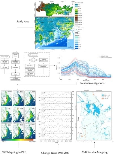
1. Introduction
2. Materials and Methods
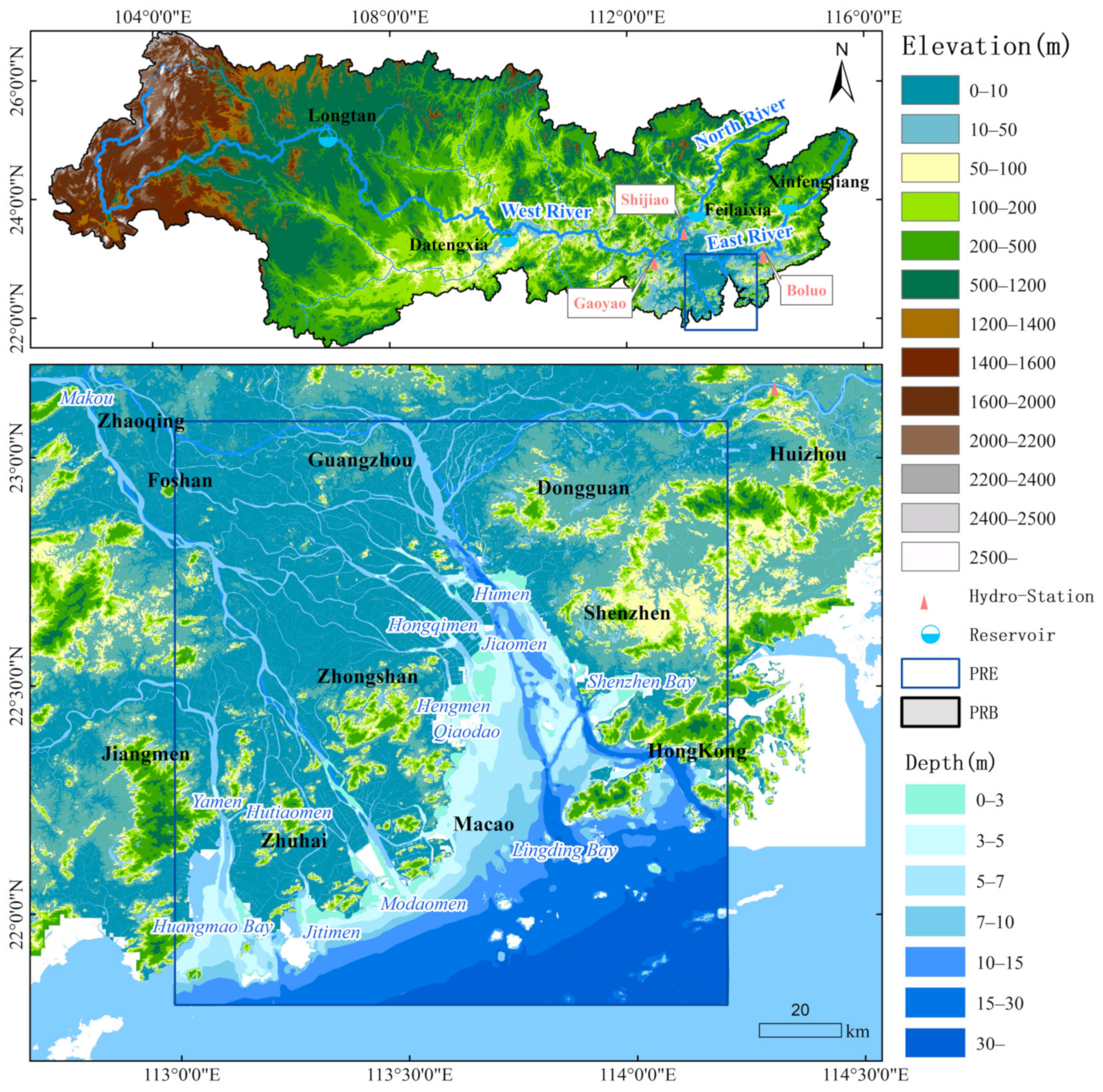
2.1. Study Area
2.2. In Situ Data Collection
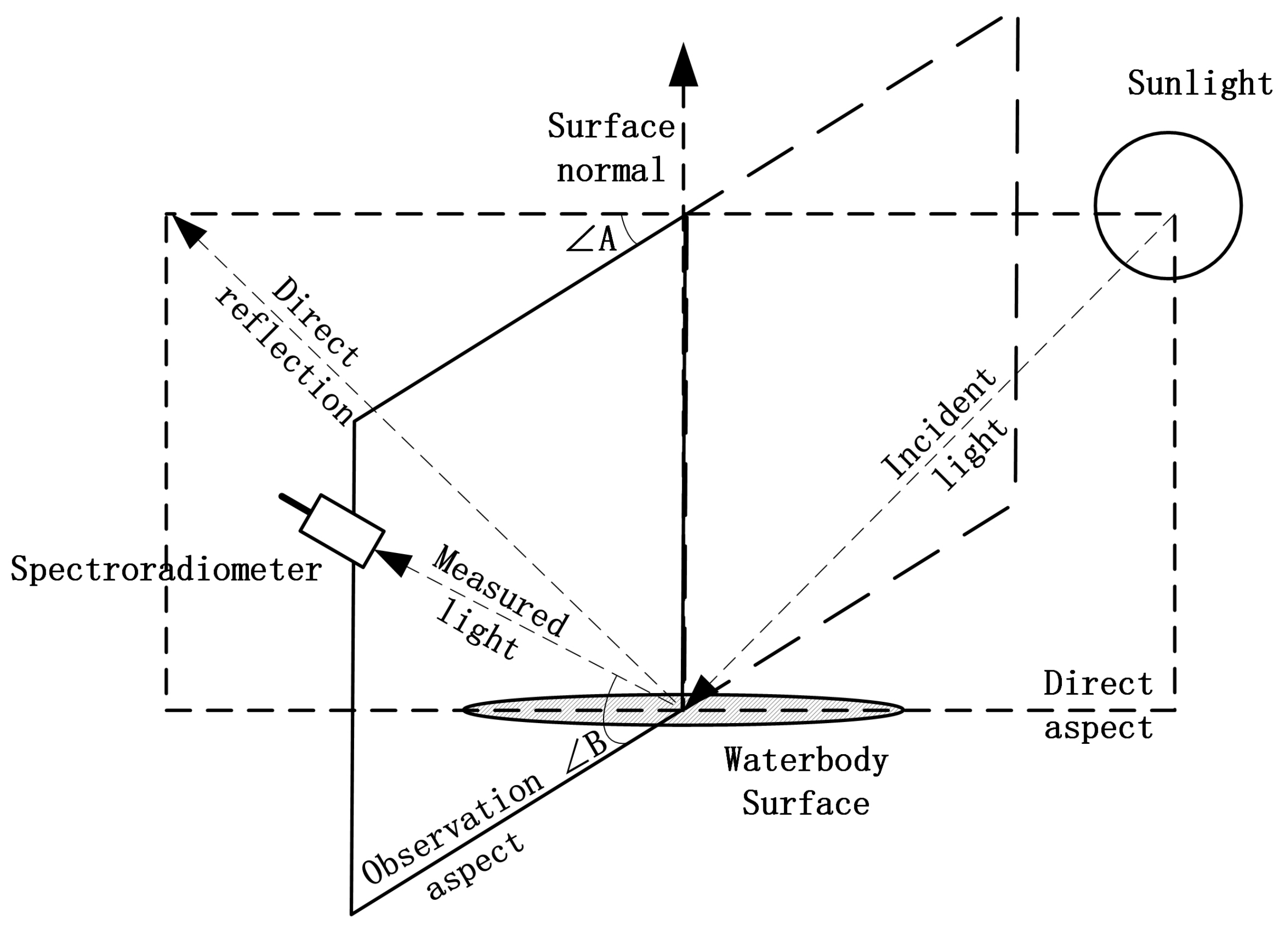
2.2.1. Normalized Water Surface Reflectance
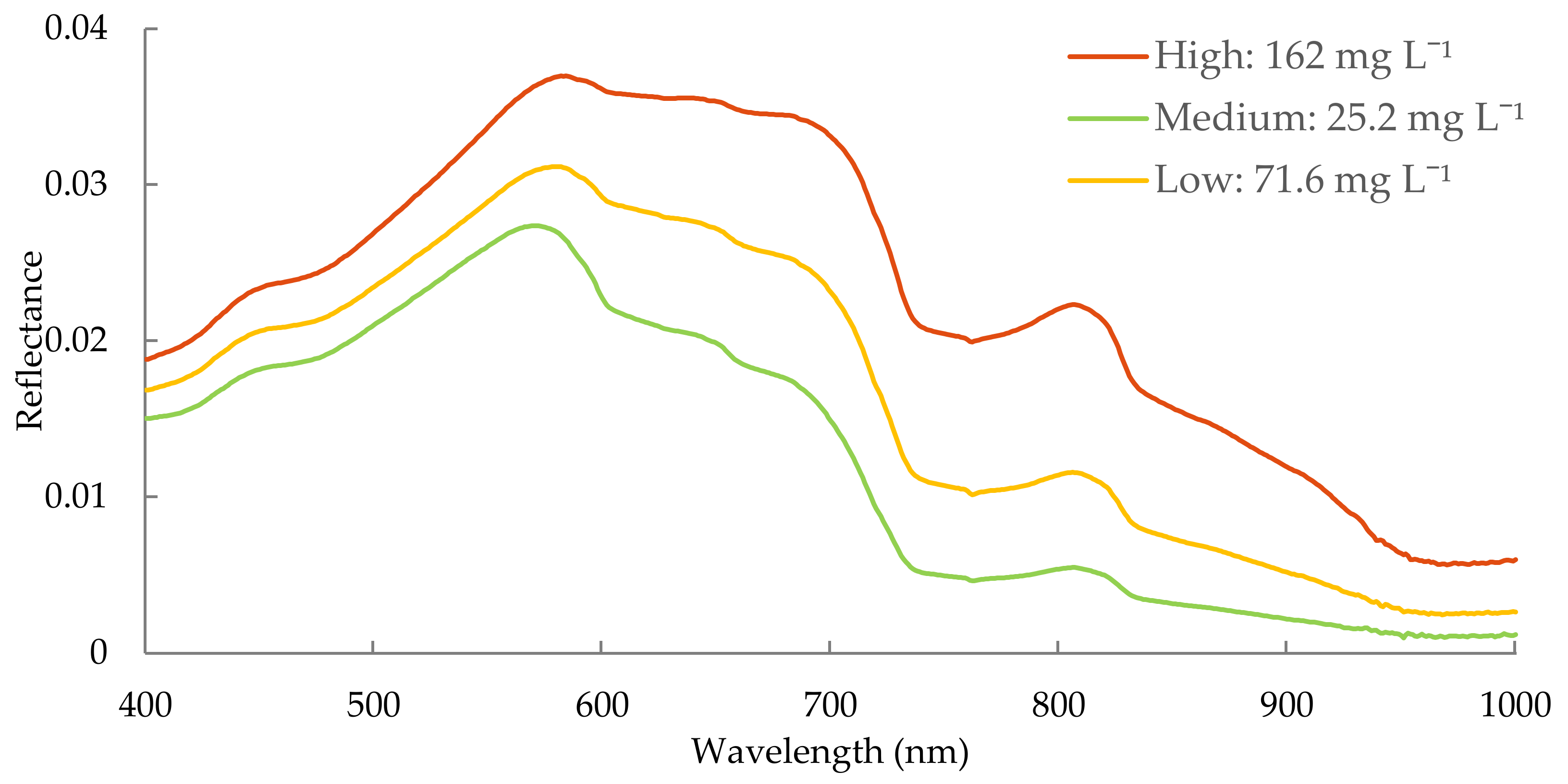
2.2.2. Spectral Characteristics of Turbid Waters
2.3. Satellite Data and Image Pre-Processing
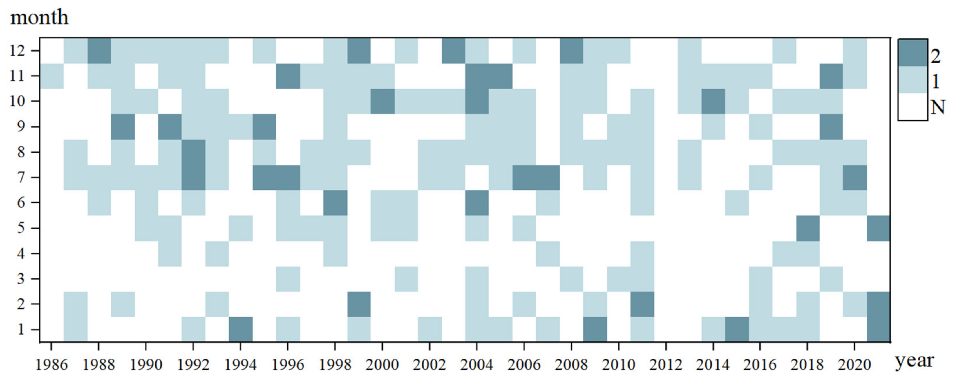
2.3.1. Satellite Data Availability
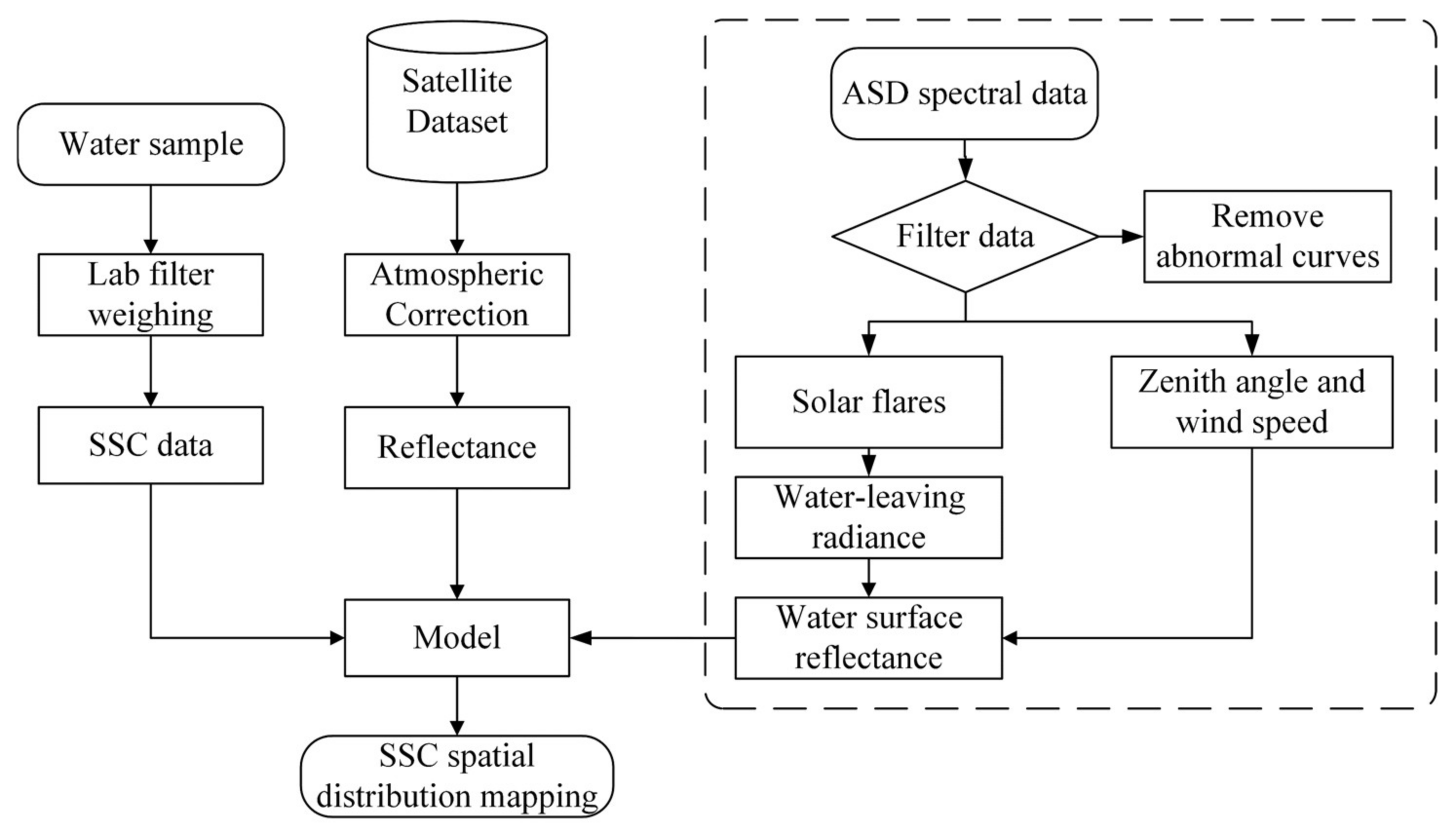
2.3.2. Satellite Image Correction
2.3.3. Mann–Kendall Trend Test
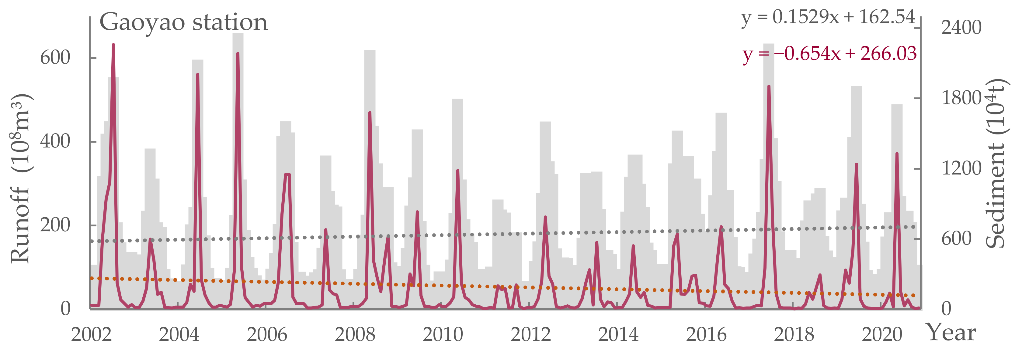
2.4. Hydrological Observations and Meteorological Data
3. Results
3.1. Spectral Characteristics of Turbid Water
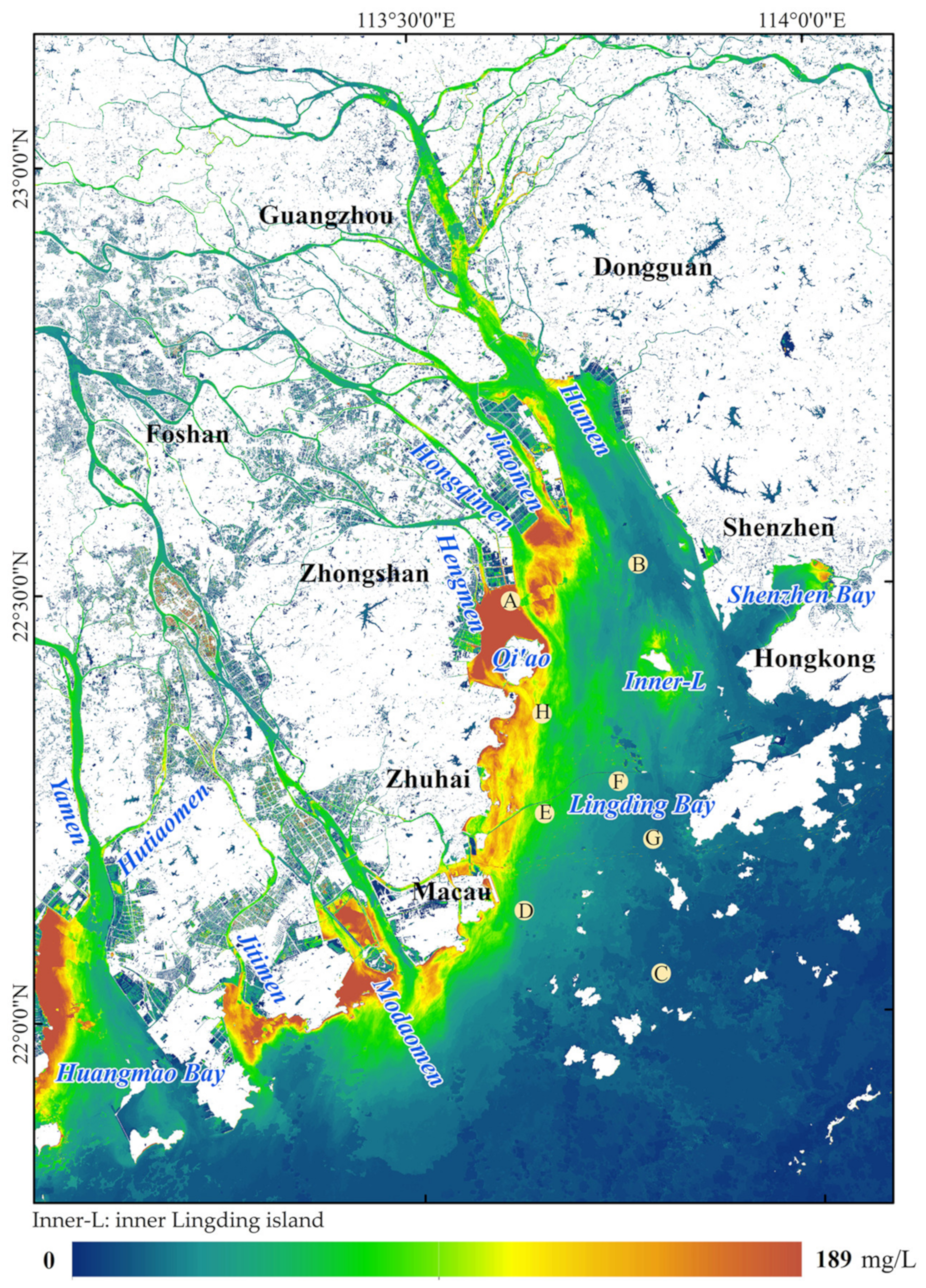
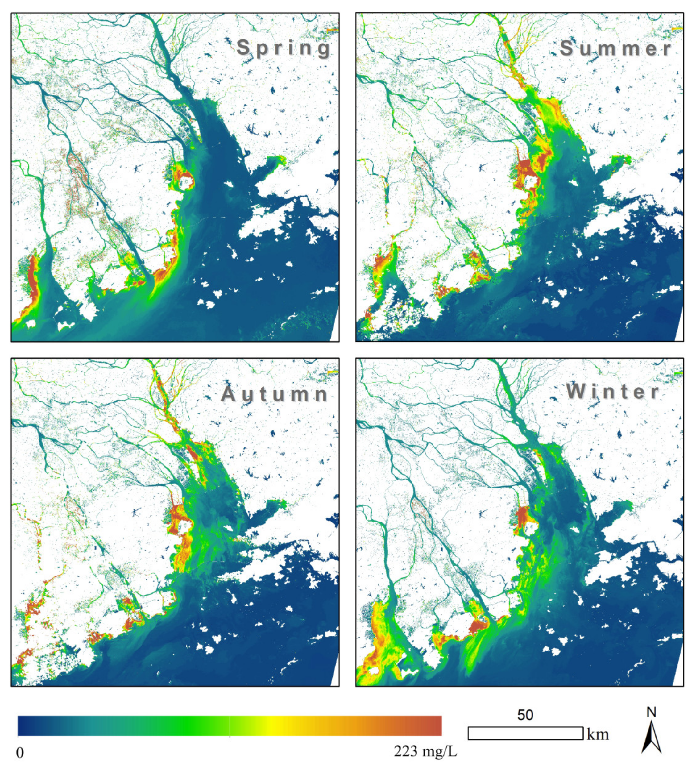
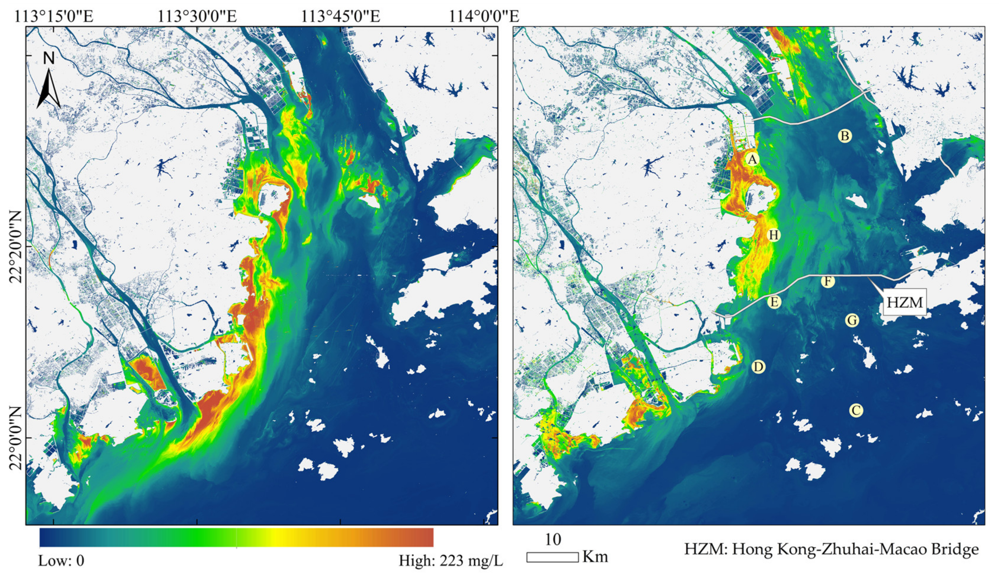
3.2. Spatial Patterns of SSC in PRE
3.3. The Long-Term Changes of SSC in PRE
3.3.1. The Distribution of Multi-Year Average SSC
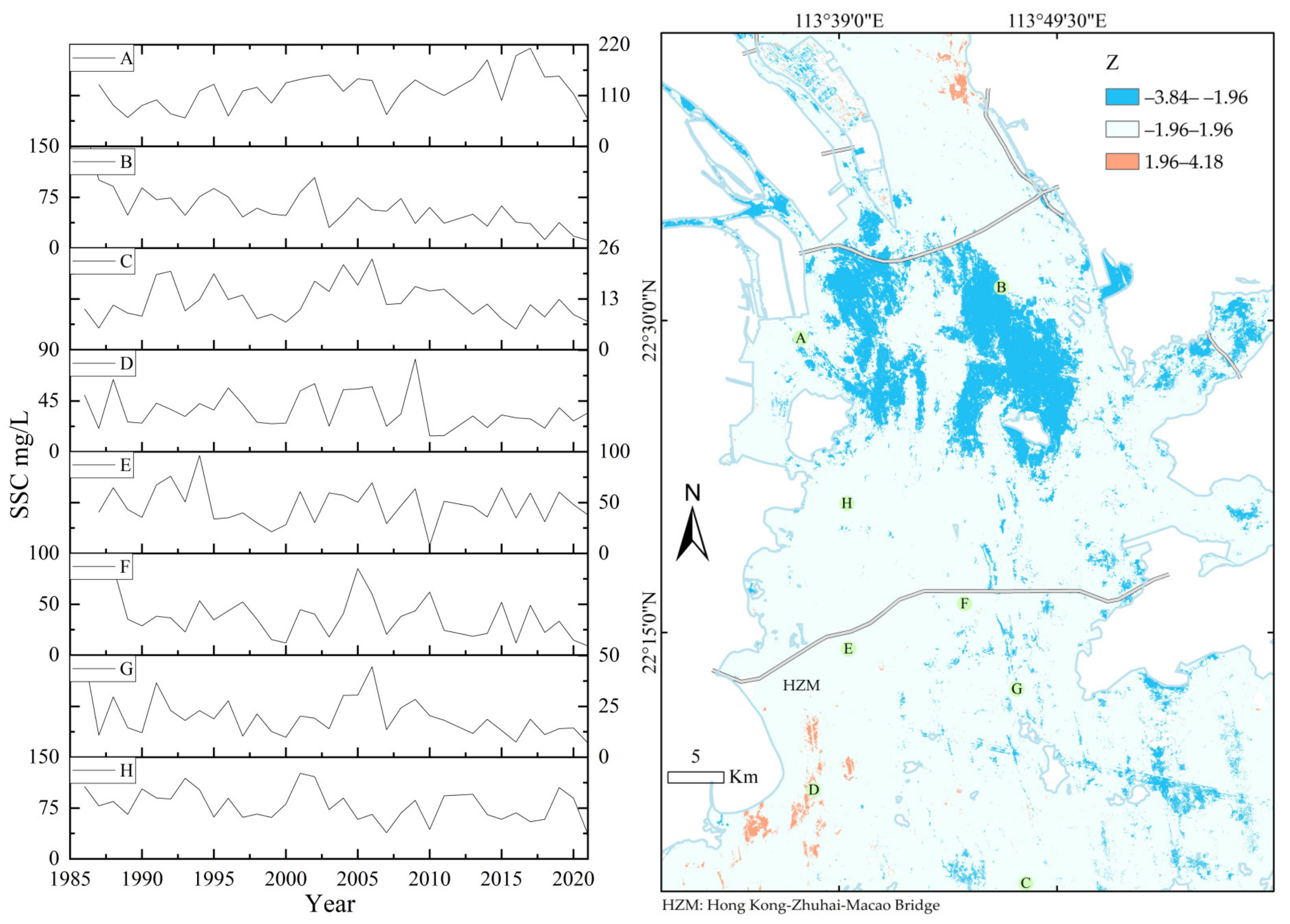
3.3.2. Mann–Kendall Test Results
4. Discussion
4.1. The Impact of Seasonal Changes
4.2. Seasonal Effects of Wind
4.3. Influence of Channel Dredging and Artificial Facilities
4.4. Uncertainty Factors in Remote Sensing Inversion
5. Conclusions
Author Contributions
Funding
Data Availability Statement
Acknowledgments
Conflicts of Interest
Appendix A

| Origin ID | Longitude | Latitude | SSC (mg L−1) |
|---|---|---|---|
| 20-07-01RS | 113°44.0 | 22°00.7 | 4.0 |
| 20-07-02RS | 113°44.7 | 22°01.6 | 39.7 |
| 20-07-03RS | 113°42.4 | 22°04.1 | 0.7 |
| 20-07-04RS | 113°40.5 | 22°06.1 | 24.3 |
| 20-07-05RS | 113°38.4 | 22°07.9 | 40.7 |
| 20-07-06RS | 113°39.7 | 22°12.9 | 32.7 |
| 20-07-07RS | 113°38.6 | 22°11.3 | 14.7 |
| 20-07-08RS | 113°37.7 | 22°09.8 | 6.3 |
| 20-07-09RS | 113°37.1 | 22°08.7 | 37.7 |
| 20-07-10RS | 113°36.4 | 22°08.0 | 49.6 |
| 20-07-11RS | 113°36.0 | 22°07.2 | 40.3 |
| 20-07-12RS | 113°35.4 | 22°06.6 | 10.0 |
| 20-07-13RS | 113°34.9 | 22°05.8 | 42.7 |
| 20-07-14RS | 113°34.5 | 22°05.0 | 47.7 |
| 20-07-15RS | 113°35.2 | 22°03.8 | 45.7 |
| 20-07-16RS | 113°35.6 | 22°03.0 | 46.7 |
| 20-07-17RS | 113°36.3 | 22°02.4 | 49.7 |
| 20-07-18RS | 113°36.8 | 22°01.8 | 44.0 |
| 20-07-19RS | 113°37.6 | 22°01.4 | 4.7 |
| 20-07-20RS | 113°38.4 | 22°01.2 | 41.3 |
| 20-07-21RS | 113°39.6 | 22°00.0 | 4.3 |
| 20-07-22RS | 113°41.0 | 21°58.9 | 1.3 |
| 20-07-23RS | 113°42.2 | 21°59.2 | |
| 20-07-24RS | 113°43.5 | 21°59.7 | 3.3 |
| 20-07-25RS | 113°37.2 | 22°11.7 | 9.3 |
| 20-07-26RS | 113°38.9 | 22°11.5 | 6.0 |
| 20-07-27RS | 113°41.5 | 22°11.1 | 33.0 |
| 20-07-28RS | 113°44.3 | 22°10.2 | 37.0 |
| 20-07-29RS | 113°45.7 | 22°10.0 | 3.3 |
| 20-07-30RS | 113°46.7 | 22°09.9 | 5.7 |
| 20-07-31RS | 113°48.0 | 22°07.8 | 53.0 |
| 20-07-32RS | 113°47.8 | 22°06.3 | 4.7 |
| 20-07-33RS | 113°47.2 | 22°04.6 | 0.7 |
| 20-07-34RS | 113°46.0 | 22°03.1 | 0.3 |
| 20-07-35RS | 113°44.8 | 22°01.7 | 1.0 |
| 20-07-36RS | 113°36.4 | 22°12.4 | 20.0 |
| 20-07-37RS | 113°35.8 | 22°13.2 | 46.0 |
| 20-07-38RS | 113°35.6 | 22°13.7 | 54.0 |
| 20-12-01RS | 113.605 | 22.207 | 278.0 |
| 20-12-02RS | 113.612 | 22.197 | 232.3 |
| 20-12-03RS | 113.631 | 22.167 | 288.0 |
| 20-12-04RS | 113.664 | 22.148 | 129.8 |
| 20-12-05RS | 113.672 | 22.187 | 169.3 |
| 20-12-06RS | 113.677 | 22.214 | 189.7 |
| 20-12-07RS | 113.684 | 22.231 | 180.3 |
| 20-12-08RS | 113.661 | 22.238 | 103.0 |
| 20-12-09RS | 113.651 | 22.26 | 162.0 |
| 20-12-10RS | 113.663 | 22.281 | 84.6 |
| 20-12-11RS | 113.672 | 22.301 | 80.3 |
| 20-12-12RS | 113.695 | 22.328 | 54.7 |
| 20-12-13RS | 113.703 | 22.361 | 53.3 |
| 20-12-14RS | 113.722 | 22.382 | 57.7 |
| 20-12-15RS | 113.699 | 22.39 | 46.2 |
| 20-12-16RS | 113.673 | 22.374 | |
| 20-12-17RS | 113.655 | 22.357 | 25.2 |
| 20-12-18RS | 113.640 | 22.338 | 74.3 |
| 20-12-19RS | 113.634 | 22.329 | 64.3 |
| 20-12-20RS | 113.632 | 22.32 | 91.7 |
| 20-12-21RS | 113.626 | 22.307 | 71.7 |
| 20-12-22RS | 113.614 | 22.293 | 88.3 |
| 20-12-23RS | 113.613 | 22.279 | |
| 21-04-01RS | 113.655° | 22.61° | 67.8 |
| 21-04-02RS | 113.695° | 22.569° | 26.6 |
| 21-04-03RS | 113.724° | 22.529° | 14.0 |
| 21-04-04RS | 113.731° | 22.463° | 10.6 |
| 21-04-05RS | 113.743° | 22.412° | 21.0 |
| 21-04-06RS | 113.746° | 22.348° | 13.6 |
| 21-04-07RS | 113.727° | 22.266° | 28.0 |
| 21-04-08RS | 113.709° | 22.208° | 23.8 |
| 21-04-09RS | 113.691° | 22.165° | 17.8 |
| 21-04-10RS | 113.686° | 22.113° | 11.6 |
| 21-04-11RS | 113.679° | 22.34° | 18.2 |
| 21-04-12RS | 113.703° | 22.70° | 25.0 |
| 21-04-13RS | 113.747° | 22.88° | / |
| 21-04-14RS | 113.751° | 22.145° | / |
| 21-04-15RS | 113.725° | 22.149° | 13.0 |
| 21-04-16RS | 113.665° | 22.184° | 19.2 |
| 21-04-17RS | 113.603° | 22.212° | 14.2 |
| 21-04-18RS | 113.609° | 22.275° | 14.2 |
| 21-04-19RS | 113.630° | 22.323° | 23.8 |
| 21-04-20RS | 113.647° | 22.356° | 14.2 |
| 21-04-21RS | 113.673° | 22.404° | 16.4 |
| 21-04-22RS | 113.699° | 22.473° | 7.4 |
| 21-04-23RS | 113.71° | 22.515° | |
| 21-04-24RS | 113.698° | 22.567° | 16.0 |
| 21-04-25RS | 113.666° | 22.596° | 15.7 |
| 21-07-01RS | 113.716° | 22.538° | 25.4 |
| 21-07-02RS | 113.698° | 22.503° | 78.2 |
| 21-07-03RS | 113.687° | 22.476° | 67.4 |
| 21-07-04RS | 113.681° | 22.435° | 29 |
| 21-07-05RS | 113.667° | 22.4° | 20.8 |
| 21-07-06RS | 113.714° | 22.441° | 18 |
| 21-07-07RS | 113.731° | 22.485° | 18 |
| 21-07-08RS | 113.733° | 22.523° | 26.2 |
| 21-07-12RS | 113.726° | 22.576° | 22.2 |
| Observation Zenith Angle (°) | Relative Observation Azimuth (°) (Water Surface as the Origin) | Relative Observation Azimuth (°) (Measuring Person as the Origin) | Wind Speed (m/s) | Sun Zenith Angle (°) | Water Surface Specular Reflectance |
|---|---|---|---|---|---|
| 40 | 45 | 135 | 0 | 10 | 0.0256 |
| 40 | 45 | 135 | 0 | 20 | 0.0256 |
| 40 | 45 | 135 | 0 | 30 | 0.0256 |
| 40 | 45 | 135 | 0 | 40 | 0.0256 |
| 40 | 45 | 135 | 0 | 50 | 0.0256 |
| 40 | 45 | 135 | 0 | 60 | 0.0256 |
| 40 | 45 | 135 | 0 | 70 | 0.0256 |
| 40 | 45 | 135 | 0 | 80 | 0.0256 |
| 40 | 45 | 135 | 2 | 10 | 0.0268 |
| 40 | 45 | 135 | 2 | 20 | 0.0265 |
| 40 | 45 | 135 | 2 | 30 | 0.0264 |
| 40 | 45 | 135 | 2 | 40 | 0.0264 |
| 40 | 45 | 135 | 2 | 50 | 0.0265 |
| 40 | 45 | 135 | 2 | 60 | 0.0265 |
| 40 | 45 | 135 | 2 | 70 | 0.0263 |
| 40 | 45 | 135 | 2 | 80 | 0.0262 |
| 40 | 45 | 135 | 4 | 10 | 0.0284 |
| 40 | 45 | 135 | 4 | 20 | 0.0278 |
| 40 | 45 | 135 | 4 | 30 | 0.0276 |
| 40 | 45 | 135 | 4 | 40 | 0.0277 |
| 40 | 45 | 135 | 4 | 50 | 0.0278 |
| 40 | 45 | 135 | 4 | 60 | 0.0277 |
| 40 | 45 | 135 | 4 | 70 | 0.0275 |
| 40 | 45 | 135 | 4 | 80 | 0.0272 |
| 40 | 45 | 135 | 6 | 10 | 0.0337 |
| 40 | 45 | 135 | 6 | 20 | 0.0297 |
| 40 | 45 | 135 | 6 | 30 | 0.029 |
| 40 | 45 | 135 | 6 | 40 | 0.0291 |
| 40 | 45 | 135 | 6 | 50 | 0.0293 |
| 40 | 45 | 135 | 6 | 60 | 0.0292 |
| 40 | 45 | 135 | 6 | 70 | 0.0289 |
| 40 | 45 | 135 | 6 | 80 | 0.0284 |
| 40 | 45 | 135 | 8 | 10 | 0.043 |
| 40 | 45 | 135 | 8 | 20 | 0.0335 |
| 40 | 45 | 135 | 8 | 30 | 0.0311 |
| 40 | 45 | 135 | 8 | 40 | 0.031 |
| 40 | 45 | 135 | 8 | 50 | 0.0312 |
| 40 | 45 | 135 | 8 | 60 | 0.0311 |
| 40 | 45 | 135 | 8 | 70 | 0.0307 |
| 40 | 45 | 135 | 8 | 80 | 0.03 |
| 40 | 90 | 90 | 0 | 10 | 0.0256 |
| 40 | 90 | 90 | 0 | 20 | 0.0256 |
| 40 | 90 | 90 | 0 | 30 | 0.0256 |
| 40 | 90 | 90 | 0 | 40 | 0.0256 |
| 40 | 90 | 90 | 0 | 50 | 0.0256 |
| 40 | 90 | 90 | 0 | 60 | 0.0256 |
| 40 | 90 | 90 | 0 | 70 | 0.0256 |
| 40 | 90 | 90 | 0 | 80 | 0.0256 |
| 40 | 90 | 90 | 2 | 10 | 0.0273 |
| 40 | 90 | 90 | 2 | 20 | 0.027 |
| 40 | 90 | 90 | 2 | 30 | 0.0267 |
| 40 | 90 | 90 | 2 | 40 | 0.0266 |
| 40 | 90 | 90 | 2 | 50 | 0.0264 |
| 40 | 90 | 90 | 2 | 60 | 0.0264 |
| 40 | 90 | 90 | 2 | 70 | 0.0263 |
| 40 | 90 | 90 | 2 | 80 | 0.0262 |
| 40 | 90 | 90 | 4 | 10 | 0.0308 |
| 40 | 90 | 90 | 4 | 20 | 0.029 |
| 40 | 90 | 90 | 4 | 30 | 0.0278 |
| 40 | 90 | 90 | 4 | 40 | 0.0275 |
| 40 | 90 | 90 | 4 | 50 | 0.0272 |
| 40 | 90 | 90 | 4 | 60 | 0.0272 |
| 40 | 90 | 90 | 4 | 70 | 0.0271 |
| 40 | 90 | 90 | 4 | 80 | 0.0269 |
| 40 | 90 | 90 | 6 | 10 | 0.0441 |
| 40 | 90 | 90 | 6 | 20 | 0.0339 |
| 40 | 90 | 90 | 6 | 30 | 0.0293 |
| 40 | 90 | 90 | 6 | 40 | 0.0288 |
| 40 | 90 | 90 | 6 | 50 | 0.0285 |
| 40 | 90 | 90 | 6 | 60 | 0.0284 |
| 40 | 90 | 90 | 6 | 70 | 0.0283 |
| 40 | 90 | 90 | 6 | 80 | 0.028 |
| 40 | 90 | 90 | 8 | 10 | 0.0617 |
| 40 | 90 | 90 | 8 | 20 | 0.0448 |
| 40 | 90 | 90 | 8 | 30 | 0.0361 |
| 40 | 90 | 90 | 8 | 40 | 0.0314 |
| 40 | 90 | 90 | 8 | 50 | 0.0308 |
| 40 | 90 | 90 | 8 | 60 | 0.0306 |
| 40 | 90 | 90 | 8 | 70 | 0.0305 |
| 40 | 90 | 90 | 8 | 80 | 0.0302 |
| 0 | 0 | 0 | 0 | 10 | 0.0211 |
| 0 | 0 | 0 | 0 | 20 | 0.0211 |
| 0 | 0 | 0 | 0 | 30 | 0.0211 |
| 0 | 0 | 0 | 0 | 40 | 0.0211 |
| 0 | 0 | 0 | 0 | 50 | 0.0211 |
| 0 | 0 | 0 | 0 | 60 | 0.0211 |
| 0 | 0 | 0 | 0 | 70 | 0.0211 |
| 0 | 0 | 0 | 0 | 80 | 0.0211 |
| 0 | 0 | 0 | 2 | 10 | 0.2239 |
| 0 | 0 | 0 | 2 | 20 | 0.0865 |
| 0 | 0 | 0 | 2 | 30 | 0.0277 |
| 0 | 0 | 0 | 2 | 40 | 0.0231 |
| 0 | 0 | 0 | 2 | 50 | 0.0224 |
| 0 | 0 | 0 | 2 | 60 | 0.0219 |
| 0 | 0 | 0 | 2 | 70 | 0.0216 |
| 0 | 0 | 0 | 2 | 80 | 0.0214 |
| 0 | 0 | 0 | 4 | 10 | 0.1667 |
| 0 | 0 | 0 | 4 | 20 | 0.1316 |
| 0 | 0 | 0 | 4 | 30 | 0.0625 |
| 0 | 0 | 0 | 4 | 40 | 0.0278 |
| 0 | 0 | 0 | 4 | 50 | 0.0236 |
| 0 | 0 | 0 | 4 | 60 | 0.0226 |
| 0 | 0 | 0 | 4 | 70 | 0.022 |
| 0 | 0 | 0 | 4 | 80 | 0.0216 |
| 0 | 0 | 0 | 6 | 10 | 0.1259 |
| 0 | 0 | 0 | 6 | 20 | 0.1388 |
| 0 | 0 | 0 | 6 | 30 | 0.0891 |
| 0 | 0 | 0 | 6 | 40 | 0.0438 |
| 0 | 0 | 0 | 6 | 50 | 0.0246 |
| 0 | 0 | 0 | 6 | 60 | 0.0232 |
| 0 | 0 | 0 | 6 | 70 | 0.0223 |
| 0 | 0 | 0 | 6 | 80 | 0.0217 |
| 0 | 0 | 0 | 8 | 10 | 0.1049 |
| 0 | 0 | 0 | 8 | 20 | 0.1276 |
| 0 | 0 | 0 | 8 | 30 | 0.1088 |
| 0 | 0 | 0 | 8 | 40 | 0.0581 |
| 0 | 0 | 0 | 8 | 50 | 0.033 |
| 0 | 0 | 0 | 8 | 60 | 0.0251 |
| 0 | 0 | 0 | 8 | 70 | 0.0233 |
| 0 | 0 | 0 | 8 | 80 | 0.0222 |
References
- Curran, P.J.; Novo, E.M.M. The Relationship Between Suspended Sediment Concentration and Remotely Sensed Spectral Radiance: A Review. J. Coast. Res. 1988, 4, 351–368. [Google Scholar] [CrossRef]
- Ritchie, J.C.; McHenry, J.R.; Schiebe, F.R.; Wilson, R.B. Relationship of reflected solar radiation and the concentration of sediment in the surface water of reservoirs. Remote Sens. Earth Resour. 1975, 3, 57–71. [Google Scholar]
- Zhan, W.; Wu, J.; Wei, X.; Tang, S.; Zhan, H. Spatio-temporal variation of the suspended sediment concentration in the Pearl River Estuary observed by MODIS during 2003–2015. Cont. Shelf Res. 2019, 172, 22–32. [Google Scholar] [CrossRef]
- Gholizadeh, M.; Melesse, A.; Reddi, L. A Comprehensive Review on Water Quality Parameters Estimation Using Remote Sensing Techniques. Sensors 2016, 16, 1298. [Google Scholar] [CrossRef]
- Stumpf, R.P.; Pennock, J.R. Calibration of a general optical equation for remote sensing of suspended sediments in a moderately turbid estuary. J. Geophys. Res. 1989, 94, 14363. [Google Scholar] [CrossRef]
- Zhang, M.; Dong, Q.; Cui, T.; Xue, C.; Zhang, S. Suspended sediment monitoring and assessment for Yellow River estuary from Landsat TM and ETM+ imagery. Remote Sens. Environ. 2014, 146, 136–147. [Google Scholar] [CrossRef]
- Luo, W.; Shen, F.; He, Q.; Cao, F.; Zhao, H.; Li, M. Changes in suspended sediments in the Yangtze River Estuary from 1984 to 2020: Responses to basin and estuarine engineering constructions. Sci. Total Environ. 2022, 805, 150381. [Google Scholar] [CrossRef]
- Wang, C.; Li, W.; Chen, S.; Li, D.; Wang, D.; Liu, J. The spatial and temporal variation of total suspended solid concentration in Pearl River Estuary during 1987–2015 based on Remote Sens. Sci. Total Environ. 2018, 618, 1125–1138. [Google Scholar] [CrossRef]
- Qiu, Z.; Xiao, C.; Perrie, W.; Sun, D.; Wang, S.; Shen, H.; Yang, D.; He, Y. Using Landsat 8 data to estimate suspended particulate matter in the Yellow River estuary: Landsat 8 spm in the yellow river estuary. J. Geophys. Res. Ocean. 2017, 122, 276–290. [Google Scholar] [CrossRef]
- Cheng, Z.; Wang, X.; Paull, D.; Gao, J. Application of the Geostationary Ocean Color Imager to Mapping the Diurnal and Seasonal Variability of Surface Suspended Matter in a Macro-Tidal Estuary. Remote Sens. 2016, 8, 244. [Google Scholar] [CrossRef]
- Peterson, K.; Sagan, V.; Sidike, P.; Cox, A.; Martinez, M. Suspended Sediment Concentration Estimation from Landsat Imagery along the Lower Missouri and Middle Mississippi Rivers Using an Extreme Learning Machine. Remote Sens. 2018, 10, 1503. [Google Scholar] [CrossRef]
- Chelotti, G.B.; Martinez, J.M.; Roig, H.L.; Olivietti, D. Space-Temporal analysis of suspended sediment in low concentration reservoir by Remote Sens. RBRH 2019, 24, 143–151. [Google Scholar] [CrossRef]
- Wu, Z.; Milliman, J.D.; Zhao, D.; Cao, Z.; Zhou, J.; Zhou, C. Geomorphologic changes in the lower Pearl River Delta, 1850–2015, largely due to human activity. Geomorphology 2018, 314, 42–54. [Google Scholar] [CrossRef]
- Qiu, J.; Cao, B.; Park, E.; Yang, X.; Zhang, W.; Tarolli, P. Flood Monitoring in Rural Areas of the Pearl River Basin (China) Using Sentinel-1 SAR. Remote Sens. 2021, 13, 1384. [Google Scholar] [CrossRef]
- Yang, X.; Lu, X.; Ran, L.; Tarolli, P. Geomorphometric Assessment of the Impacts of Dam Construction on River Disconnectivity and Flow Regulation in the Yangtze Basin. Sustainability 2019, 11, 3427. [Google Scholar] [CrossRef]
- Yang, X.; Lu, X.X. Estimate of cumulative sediment trapping by multiple reservoirs in large river basins: An example of the Yangtze River basin. Geomorphology 2014, 227, 49–59. [Google Scholar] [CrossRef]
- Wu, Z.; Zhao, D.; Syvitski, J.P.M.; Saito, Y.; Zhou, J.; Wang, M. Anthropogenic impacts on the decreasing sediment loads of nine major rivers in China, 1954–2015. Sci. Total Environ. 2020, 739, 139653. [Google Scholar] [CrossRef]
- Li, P.; Ke, Y.; Bai, J.; Zhang, S.; Chen, M.; Zhou, D. Spatiotemporal dynamics of suspended particulate matter in the Yellow River Estuary, China during the past two decades based on time-series Landsat and Sentinel-2 data. Mar. Pollut. Bull. 2019, 149, 110518. [Google Scholar] [CrossRef]
- Gao, F.; Wang, Y.; Hu, X. Evaluation of the suitability of Landsat, MERIS, and MODIS for identifying spatial distribution patterns of total suspended matter from a self-organizing map (SOM) perspective. CATENA 2019, 172, 699–710. [Google Scholar] [CrossRef]
- Du, Y.; Lin, H.; He, S.; Wang, D.; Wang, Y.P.; Zhang, J. Tide-Induced Variability and Mechanisms of Surface Suspended Sediment in the Zhoushan Archipelago along the Southeastern Coast of China Based on GOCI Data. Remote Sens. 2021, 13, 929. [Google Scholar] [CrossRef]
- Mao, Q.; Shi, P.; Yin, K.; Gan, J.; Qi, Y. Tides and tidal currents in the Pearl River Estuary. Cont. Shelf Res. 2004, 24, 1797–1808. [Google Scholar] [CrossRef]
- Dai, S.B.; Yang, S.L.; Cai, A.M. Impacts of dams on the sediment flux of the Pearl River, southern China. CATENA 2008, 76, 36–43. [Google Scholar] [CrossRef]
- Ou, S.; Yang, Q.; Luo, X.; Zhu, F.; Luo, K.; Yang, H. The influence of runoff and wind on the dispersion patterns of suspended sediment in the Zhujiang (Pearl) River Estuary based on MODIS data. Acta Oceanol. Sin. 2019, 38, 26–35. [Google Scholar] [CrossRef]
- Mobley, C.D. Estimation of the remote-sensing reflectance from above-surface measurements. Appl. Opt. 1999, 38, 7442. [Google Scholar] [CrossRef] [PubMed]
- Tang, J.; Tian, G.; Wang, X. Spectral Measurement and Analysis of Water I: Above-water Measurement. Natl. Remote Sens. Bull. 2004, 8, 37–44. [Google Scholar]
- Li, H.; Xie, X.; Yang, X.; Cao, B.; Xia, X. An Integrated Model of Summer and Winter for Chlorophyll-a Retrieval in the Pearl River Estuary Based on Hyperspectral Data. Remote Sens. 2022, 14, 2270. [Google Scholar] [CrossRef]
- Zhao, J.; Zhang, F.; Chen, S.; Wang, C.; Chen, J.; Zhou, H.; Xue, Y. Remote Sensing Evaluation of Total Suspended Solids Dynamic with Markov Model: A Case Study of Inland Reservoir across Administrative Boundary in South China. Sensors 2020, 20, 6911. [Google Scholar] [CrossRef]
- Jia, Q.; Zhang, G.; Tang, S.; Zhang, H. Analysis on seasonal changes of suspended sediment in Lingdingyang waters of the Pearl River Estuary from 2013 to 2018. J. Sun Yat-Sen Univ. 2021, 60, 59–71. [Google Scholar] [CrossRef]
- Wang, J.-J.; Lu, X.X.; Liew, S.C.; Zhou, Y. Retrieval of suspended sediment concentrations in large turbid rivers using Landsat ETM+: An example from the Yangtze River, China. Earth Surf. Processes Landf. 2009, 34, 1082–1092. [Google Scholar] [CrossRef]
- Collins, M.; Pattiaratchi, C. Identification of suspended sediment in coastal waters using airborne thematic mapper data. Int. J. Remote Sens. 1984, 5, 635–657. [Google Scholar] [CrossRef]
- Islam, M.R.; Yamaguchi, Y.; Ogawa, K. Suspended sediment in the Ganges and Brahmaputra Rivers in Bangladesh: Observation from TM and AVHRR data. Hydrol. Processes 2001, 15, 493–509. [Google Scholar] [CrossRef]
- Wang, S.; Li, J.; Zhang, B.; Shen, Q.; Zhang, F.; Lu, Z. A simple correction method for the MODIS surface reflectance product over typical inland waters in China. Int. J. Remote Sens. 2016, 37, 6076–6096. [Google Scholar] [CrossRef]
- MWR.CN. China River Sediment Bulletin 2001–2020. 2021. Available online: http://www.pearlwater.gov.cn/zwgkcs/lygb/nsgb/202111/P020211126575293575253.pdf (accessed on 12 June 2022).
- Zhang, S.; Lu, X.X.; Higgitt, D.L.; Chen, C.-T.A.; Han, J.; Sun, H. Recent changes of water discharge and sediment load in the Zhujiang (Pearl River) Basin, China. Glob. Planet Chang. 2008, 60, 365–380. [Google Scholar] [CrossRef]
- Wu, C.S.; Yang, S.L.; Lei, Y.-P. Quantifying the anthropogenic and climatic impacts on water discharge and sediment load in the Pearl River (Zhujiang), China (1954–2009). J. Hydrol. 2012, 452–453, 190–204. [Google Scholar] [CrossRef]
- Scully, M.E.; Friedrichs, C.; Brubaker, J. Control of estuarine stratification and mixing by wind-induced straining of the estuarine density field. Estuaries 2005, 28, 321–326. [Google Scholar] [CrossRef]
- Zhou, Y.; Xuan, J.; Huang, D. Tidal variation of total suspended solids over the Yangtze Bank based on the geostationary ocean color imager. Sci. China Earth Sci. 2020, 63, 1381–1389. [Google Scholar] [CrossRef]
- Wu, Z.Y.; Saito, Y.; Zhao, D.N.; Zhou, J.Q.; Cao, Z.Y.; Li, S.J.; Shang, J.H.; Liang, Y.Y. Impact of human activities on subaqueous topographic change in Lingding Bay of the Pearl River estuary, China, during 1955–2013. Sci. Rep. 2016, 6, 37742. [Google Scholar] [CrossRef]
- Chen, J.; Chen, S.; Fu, R.; Li, D.; Jiang, H.; Wang, C.; Peng, Y.; Jia, K.; Hicks, B.J. Remote Sensing Big Data for Water Environment Monitoring: Current Status, Challenges, and Future Prospects. Earth’s Future 2022, 10, e2021EF002289. [Google Scholar] [CrossRef]


| Year | Type | Gaoyao | Shijiao | Boluo | Total of PR |
|---|---|---|---|---|---|
| Average from 1954 to 2020 | Runoff | 2186 | 417.8 | 232 | 3419 |
| Sediment load | 5650 | 525 | 217 | 7400 | |
| Average in the past 10 years | runoff | 2212 | 421 | 223.7 | - |
| Sediment load | 1740 | 464 | 91.4 | - | |
| 2019 | runoff | 2397 | 537.1 | 270.6 | 3972 |
| Sediment load | 2460 | 488 | 160 | 3320 | |
| 2020 | runoff | 2173 | 364 | 157.1 | 3085 |
| Sediment load | 1830 | 404 | 44.3 | 2770 |
| ID | Sediment (mg) | Filter Paper (mg) | Sample Weight (mL) | SSC (mg L−1) |
|---|---|---|---|---|
| 1 | 85.1 | 131.7 | 300 | 278.0 |
| 2 | 70.7 | 131.3 | 300 | 232.3 |
| 3 | 87.1 | 132.5 | 300 | 288.0 |
| 4 | 65.4 | 132.7 | 500 | 129.8 |
| 5 | 50.8 | 132.1 | 300 | 167.7 |
| 6 | 66.4 | 131.2 | 350 | 189.7 |
| 7 | 54.1 | 131.4 | 300 | 179.0 |
| 8 | 30.9 | 133.5 | 300 | 103.0 |
| 9 | 48.6 | 131.6 | 300 | 162.0 |
| 10 | 42.3 | 132.9 | 500 | 84.6 |
| 11 | 24.1 | 131.4 | 300 | 80.3 |
| 12 | 16.4 | 133.4 | 300 | 54.7 |
| 13 | 16.0 | 131.1 | 300 | 53.3 |
| Band | Models | R2 | RMSE | RE |
|---|---|---|---|---|
| Landsat OLI B4 | y = 189.87x − 40.873 | R² = 0.55 | 21.29 | 95.07% |
| Y = 3.501e4.317x | R² = 0.69 | 8.28 | 18.98% | |
| Landsat OLI (B3 + B4)/(B3/B4) | y = 195.67x − 26.19 | R² = 0.70 | 26.63 | 84.90% |
| y = 4.6e4.227x | R² = 0.79 | 7.17 | 17.62% |
| Point Name | Trend | P | Z |
|---|---|---|---|
| A | increasing | 0.01 | 2.57 |
| B | decreasing | 0.001 | −4.18 |
| C | no trend | 0.42 | −0.80 |
| D | no trend | 0.37 | −0.88 |
| E | no trend | 0.57 | −0.56 |
| G | no trend | 0.14 | −1.48 |
| H | decreasing | 0.09 | −1.71 |
Publisher’s Note: MDPI stays neutral with regard to jurisdictional claims in published maps and institutional affiliations. |
© 2022 by the authors. Licensee MDPI, Basel, Switzerland. This article is an open access article distributed under the terms and conditions of the Creative Commons Attribution (CC BY) license (https://creativecommons.org/licenses/by/4.0/).
Share and Cite
Cao, B.; Qiu, J.; Zhang, W.; Xie, X.; Lu, X.; Yang, X.; Li, H. Retrieval of Suspended Sediment Concentrations in the Pearl River Estuary Using Multi-Source Satellite Imagery. Remote Sens. 2022, 14, 3896. https://doi.org/10.3390/rs14163896
Cao B, Qiu J, Zhang W, Xie X, Lu X, Yang X, Li H. Retrieval of Suspended Sediment Concentrations in the Pearl River Estuary Using Multi-Source Satellite Imagery. Remote Sensing. 2022; 14(16):3896. https://doi.org/10.3390/rs14163896
Chicago/Turabian StyleCao, Bowen, Junliang Qiu, Wenxin Zhang, Xuetong Xie, Xixi Lu, Xiankun Yang, and Haitao Li. 2022. "Retrieval of Suspended Sediment Concentrations in the Pearl River Estuary Using Multi-Source Satellite Imagery" Remote Sensing 14, no. 16: 3896. https://doi.org/10.3390/rs14163896
APA StyleCao, B., Qiu, J., Zhang, W., Xie, X., Lu, X., Yang, X., & Li, H. (2022). Retrieval of Suspended Sediment Concentrations in the Pearl River Estuary Using Multi-Source Satellite Imagery. Remote Sensing, 14(16), 3896. https://doi.org/10.3390/rs14163896