Oil Spill Detection with Dual-Polarimetric Sentinel-1 SAR Using Superpixel-Level Image Stretching and Deep Convolutional Neural Network

Abstract

Synthetic aperture radar (SAR) has been widely applied in oil spill detection on the sea surface due to the advantages of wide area coverage, all-weather operation, and multi-polarization characteristics. Sentinel-1 satellites can provide dual-polarized SAR data, and they have high potential for successful application to oil spill detection. However, the characteristics of the sea surface and oil film on different images are not the same when imaging at different locations and in different conditions, which leads to the inconsistent accuracy of these images with the application of the current oil spill detection methods. In order to avoid the above limitation, we propose an oil spill detection method using image stretching based on superpixels and a convolutional neural network. Experiments were carried out on eight Sentinel-1 dual-pol data, and the optimal superpixel number and image stretching parameters are discussed. Mean intersection over union (MIoU) was used to evaluate classification accuracy. The proposed method could effectively improve the classification accuracy; when the expansion and inhibition coefficients of image stretching were set to 1.6 and 1.2 respectively, the experiments achieved a maximum MIoU of 85.4%, 7.3% higher than that without image stretching.

1. Introduction

Crude oil leakage is one of the most influential marine pollution forms due to its difficult elimination. On 20 April 2010, an explosion accident at the drilling platform of British Petroleum occurred in the Gulf of Mexico. The sunken platform leaked about 5000 barrels of crude oil every day, representing one of the most serious ecological disasters in the history of the United States [1]. The rapid and accurate detection of oil spill is of great significance to protect marine environments and reduce economic loss.

Synthetic aperture radar (SAR) can work in all weather conditions and all day; thus, it has been widely applied in oil spill detection. The SAR sensor emits electromagnetic waves and receives echoes. The oil slick floating on the sea surface will suppress capillary gravity waves and short gravity waves, which affect the Bragg scattering of microwaves and reduce the normalized radar backscatter cross-section (NRCS), representing the intensity of radar backscattering [2]. Therefore, oil films are usually observed as dark spots on SAR images. However, many other factors also appear as dark spots in SAR images, and they could be confused with oil spill areas. These include low wind speed, biogenic oil film, plankton, waves, and rain cells, which can result in false detection. Thus, the challenge of oil spill detection is to distinguish oil spill areas from these look-alike areas [3].

Research on oil spill detection using SAR sensors began in the 1990s. Early oil spill detection is usually based on texture analysis of single polarimetric SAR images. Solberg et al. summarized oil spill detection in three steps: (1) dark spots recognition, (2) feature extraction, and (3) oil spill detection [4]. They extracted 12 texture features from the dark spots obtained from ENVISAT, Radarsat, and ERS SAR data, and the oil spill areas were successfully separated from other similar areas using a Bayesian classifier [4,5]. In 2013, Pineda et al. proposed a texture classification neural network (TCCNA) and achieved high accuracy in detecting the Gulf of Mexico oil spill [6]. Cheng et al. [7] used VV channel data acquired from COSMO-SkyMed to perform oil spill monitoring and tracking through model simulations. In 2014, Diego et al. [8] developed a tool that could offer an integrated framework for the detection and localization of marine spills with fuzzy clustering and wavelets. The PRIMI pilot project of Italy [9] developed a set of oil spill detection algorithms using texture analysis and deep learning, which achieved good monitoring results. Ajadi et al. [10,11] introduced Lipschitz regularity and multiscale change detection techniques into oil spill detection. These methods mainly focused on the extraction of geometric and texture features of dark spots in SAR images.

The main shortcoming of oil spill detection based on single-pol SAR images is that there is little chance to distinguish look-alike areas from oil spills. By contrast, the polarized information of SAR images can avoid this problem. Several polarization decomposition methods have been applied in oil spill detection with quad- or dual-polarimetric SAR data, such as Cloude decomposition and single-bounce eigenvalue relative difference (SERD) [12,13,14,15]. Skrunes et al. [16] proved that the geometric intensity and the real part of the co-polarization cross-product of C-band SAR data could distinguish well between biogenic slicks and mineral oil types. Li et al. analyzed the polarimetric scattering properties of oil-covered water using ellipticity parameters and the degree of polarization. They revealed that the main scattering mechanism of oil seep is even bounce scattering, whereas oil spill is dominated by Bragg scattering [17]. Salberg et al. [18,19] evaluated several polarized parameters and classifiers with the use of hybrid polarimetric SAR for oil spill detection. Ivonin et al. [20] generalized C-band Radarsat-2 and TerraSAR-X data using resonant to non-resonant signal damping (RND), and the method could separate mineral oil slicks from other oil slicks. Espeseth et al. [21] examined system additive and multiplicative noise on the X-, C-, and L-band SAR data covering oil slicks. The results proved that the SNR from TerraSAR-X and Radarsat-2 below 0 dB was not suitable for analysis of the scattering properties. In 2021, Li et al. [22] designed improved polarimetric feature parameters on the basis of polarimetric scattering entropy and anisotropy, and the proposed features could indicate the oil slick information and effectively suppress sea clutter and look-alike information.

With the rise of machine learning in recent years, deep learning and computer vision algorithms have gradually been applied to polarimetric SAR oil spill detection. Oil spill detection is essentially a classification problem. Accordingly, current studies on oil spill detection based on deep learning methods typically divide SAR images into fixed sizes, and then apply a convolutional neural network (CNN) model or derived semantic segmentation for classification. Many classical model structures, including fully convolutional network (FCN), U-Net, PSPNet, DeepLab series, and object-contextual representations (ORC) [23,24,25,26,27,28], are widely applied in image classification. On this basis, in oil spill detection, Zeng et al. [29] proposed a classification network named OSCNet based on vgg-16, improving the accuracy to 92.5% on specific datasets. In 2018, Yu et al. [30] introduced the f-divergence loss function into a generative adversarial network model, and it accurately segmented different shapes of oil spills in SAR images. Bianchi et al. [31] designed a deep learning framework using dense blocks to distinguish oil and non-oil areas. Zhang et al. [32] proposed a method using an advanced convolutional neural network based on the superpixel model applied to quad-polarimetric SAR images, and it led to the highest MIoU of 90.5%. Since the size and area of oil spill dark spots are different, multiscale learning methods have attracted more attention in recent years [33,34], which use multiple convolution kernels with different receptive fields to process input images for feature extraction. Zhu et al. [35] proposed the oil spill contextual and boundary-supervised detection network (CBD-Net) to extract refined oil spill regions by fusing multiscale features, and the spatial and channel squeeze excitation (scSE) block was also introduced to further improve the accuracy.

The Sentinel-1 satellite carries C-band SAR sensors. It provides single- or dual-polarimetric SAR data with large swath width. In recent years, it was widely used, and many achievements were made in geohazard detection [36,37], infrastructure deformation monitoring [38,39,40], etc. In the field of oil spill detection, Setiani et al. [41] analyzed the Balikpapan oil spill accidents that happened in 2018. Using several types of index, oil spill areas were separated from clean sea. Rajendran et al. used the parallelepiped supervised algorithm and confusion matrix to detect oil spill patches from the Wakashio oil spill accidents [42]. Naz et al. [43] analyzed four oil spill events over the Indian Ocean using Sentinel-1 data, and the spread of oil spills could be observed. Moreover, Diego et al. [44] proved that the convolutional neural network achieved higher accuracy with lower computing time, compared with clustering and logistic regression algorithms. Chaturvedi et al. [45] detected oil slicks near the Al Khafji zone using Sentinel-1 C-band SAR data. Corcione et al. [46] found that the largest deviation was observed over oil slicks using the azimuth auto correlation function (AACF). Krestenitis et al. [47] proposed a benchmark based on deep neural networks for future oil spill detection, and they found that DeepLabv3+ presented the best performance in experiments. Ma et al. [48] combined the polarized information of Sentinel-1 dual-pol SAR data with the deep learning algorithm, took the pseudo color image calculated from the polarized information as the input of the neural network, and improved the DeepLabV3+ model. The final oil spill detection accuracy rate was increased to 98.92%. In 2022, Dong et al. [49] analyzed 563,705 Sentinel-1 images from 2014 to 2019. They found that the proportion of anthropogenic discharges was an order-of-magnitude greater than natural seepages by quantifying oil slick area, and they provided a detailed global inventory of static and persistent sources.

However, the final accuracy of oil spill detection algorithms based on deep learning is highly dependent on the consistency of the training and test sets. In real applications, there are imaging differences when using different SAR data due to different imaging time and locations, leading to the inconsistent accuracy of oil spill detection among different data, which is usually much lower than normal accuracy [31,47]. In order to further improve accuracy and address the above problem, we propose an image stretching method based on SLIC superpixels and a convolutional neural network, which can enlarge the features of oil spill areas, making it possible to achieve better detection accuracy in datasets with imaging differences. Moreover, we designed a semantic segmentation model for classification. Experiments were carried out on eight Sentinel-1 dual-pol data. Two polarization decomposition methods were applied, namely, H/Alpha decomposition and Stokes parameters. The experimental results showed that the maximum MIoU achieved was 85.4% when using polarized parameters with the image stretching method, representing a 7.3% improvement in accuracy compared with the method without image stretching. The proposed method could significantly improve the accuracy of oil spill detection and alleviate the inconsistent accuracy caused by imaging differences.

2. Materials and Methods

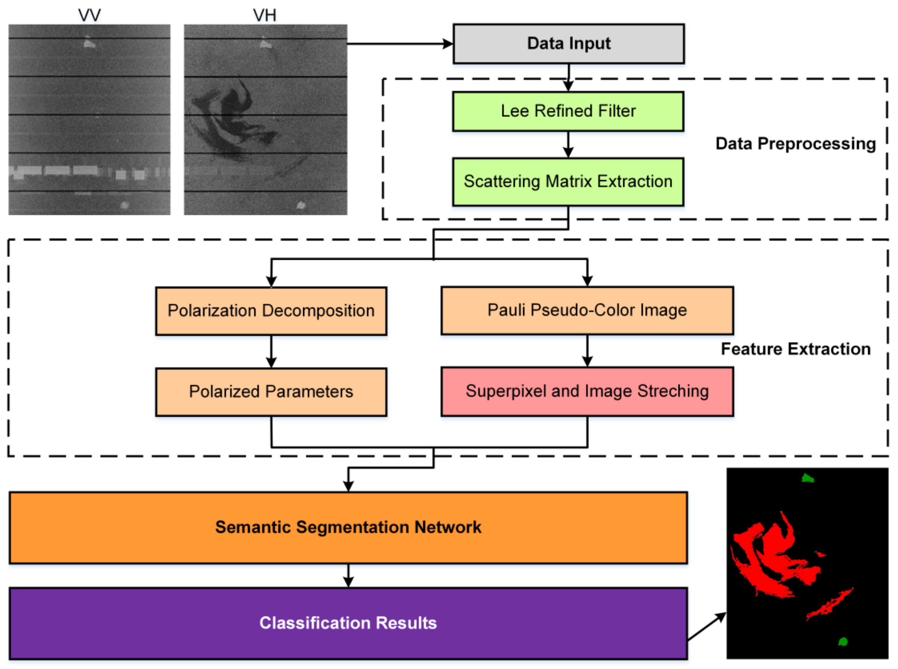
The flowchart of the proposed method is illustrated in Figure 1. The SAR data were firstly processed using the refined Lee filter, and the polarimetric parameters were calculated. The Pauli pseudo-color image was applied to calculate the SLIC superpixels. Then, the image stretching method was applied to process the SLIC superpixel results. Subsequently, the polarimetric parameters and the image stretching results were used as inputs to the constructed neural network model for training and testing. Finally, the classification results were extracted as the outputs of the model.

2.1. Polarization Decomposition

The Sentinel-1 satellite provides two types of dual-pol SAR data: VV/VH and HH/HV. This paper used VV/VH data to extract two groups of polarized parameters: H/Alpha decomposition and Stokes parameters, as shown in Figure 2.

For VV/VH data, the scattering matrix of polarimetric SAR represents the statistics of actual values of multiple scattering centers. The covariance matrix C and coherence matrix T can be used to measure the statistical characteristics and calculate polarized parameters for more accurate data analysis. The scattering matrix can be vectorized as follows:

$$K_{2L}={\left[\begin{array}{cc}{S}_{VH}& S_{VV}\end{array}\right]}^T,$$

(1)

$$K_{2P}={\left[\begin{array}{cc}{S}_{VV}& \frac{\left(1+i\right)S_{VH}}{\sqrt{2}}\end{array}\right]}^T.$$

(2)

K_2L and K_2P are treated by the inner product with their conjugate transpose matrix, and the covariance matrix C and coherence matrix T can be expressed as

$$C_2=\left[\begin{array}{cc}〈{\left|S_{VH}\right|}^2〉& 〈\left(1+i\right)S_{VH}{S}_{VH}{}^{\ast }〉\\ 〈\left(1+i\right)S_{VV}{S}_{VH}{}^{\ast }〉& 〈{\left|S_{VV}\right|}^2〉\end{array}\right] ,$$

(3)

$$T_2=\frac{1}{2}\left[\begin{array}{cc}〈2{\left|S_{VV}\right|}^2〉& 〈\left(1+i\right)S_{VH}{S}_{VV}{}^{\ast }〉\\ 〈\left(1+i\right)S_{VV}{S}_{VH}{}^{\ast }〉& 〈{\left|S_{VH}\right|}^2〉\end{array}\right].$$

(4)

By calculating eigenvalues λ₁ and λ₂ of matrix T₂, the components of each eigenvector can be defined as

$$P_i=\frac{{\lambda }_i}{{\displaystyle \sum _{j=1}^2{\lambda }_j}}.$$

(5)

Therefore, entropy (H) is defined as

$$H=-{\displaystyle \sum _{i=1}^2{P}_i{\log }_2(P_i)}.$$

(6)

The mean scattering angle (α) is calculated by

$$\alpha ={\alpha }_1{P}_1+{\alpha }_2{P}_2.$$

(7)

H, α, λ₁, and λ₂ are the four components in H/Alpha decomposition, used as H/Alpha/λ₁/λ₂ parameters.

The Stokes vector is a decomposition method for describing partially polarized waves [50,51]. The polarization state of plane waves is usually represented by wave parameter sets (g₀, g₁, g₂, g₃) as follows:

$$g=\left(\begin{array}{l}{g}_0\\ g_1\\ g_2\\ g_3\end{array}\right)=\left(\begin{array}{c}{\left|E_h\right|}^2+{\left|E_v\right|}^2\\ {\left|E_h\right|}^2-{\left|E_v\right|}^2\\ 2\mathrm{Re}(E_h{E}_v{}^{*})\\ -2\mathrm{Im}(E_h{E}_v{}^{*})\end{array}\right),$$

(8)

where E_h and E_v represent the electromagnetic vector components in the H and V directions, respectively; it can be seen from the formula that g₀² = g₁² + g₂² + g₃². Physically, g₀ is equal to the total power of plane wave and is proportional to the total amplitude, g₁ represents the amplitude difference between H and V direction components, and g₂ and g₃ are the phase difference between them. The plane wave contains a polarization component if any parameter is not equal to 0. This paper defined a new parameter contrast = g₁/g₀, with contrast/g₀/g₁/g₂/g₃ parameters set as the group of Stokes parameters.

2.2. Neural Network Model

The construction of the convolutional neural network incorporated Resblock. The idea of Resblock is to add a part to the basic neural network structure, so that it can learn the residual information between the input and output of the convolution layer [52]. Assuming that the convolution layer is represented by H and the characteristic layer of the input convolution layer is x, and the output of the convolution layer is denoted by H(x); hence, the operation process of convolution layer is to establish the mapping from X to H(x). The residual of the convolution layer is defined as

$$F\left(x\right)=H\left(x\right)-x.$$

(9)

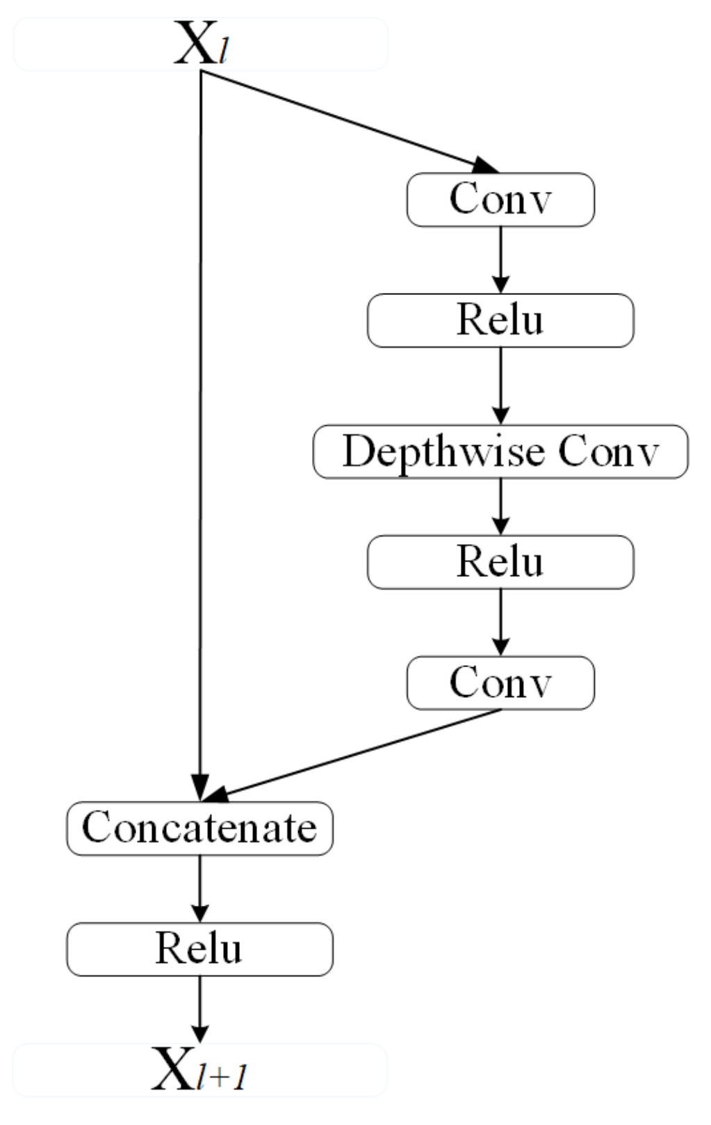
ResNet adopts Resblock to realize residual learning. Figure 3 shows the Resblock structure used in this paper, where the input tensor was calculated using two convolutional layers and a depthwise separable convolutional layer, and the calculated tensor was finally connected with the input tensor.

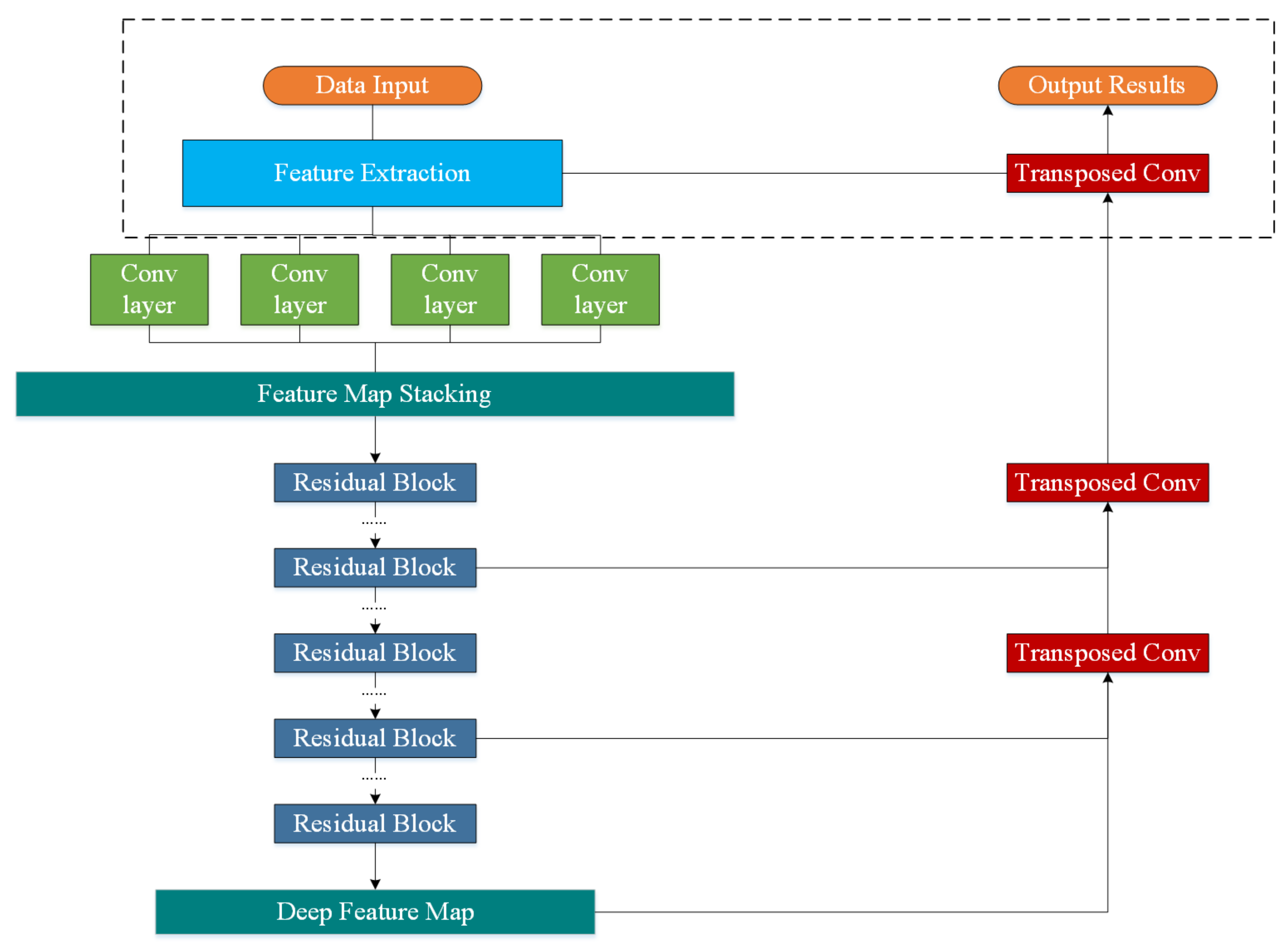
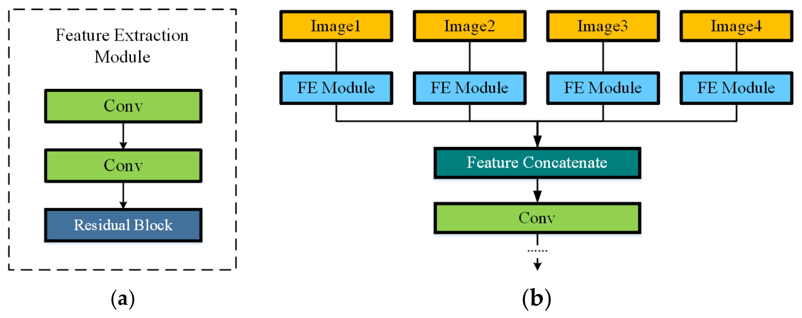
The basic structure of the semantic segmentation model is shown in Figure 4. The input training data are first processed by a feature extraction step. The extracted feature maps pass through four different scales of dilated convolution layers, before being further calculated by multiple Resblocks to obtain highly extracted feature maps. These feature maps are inversed to the same size as the inputs via several transposed convolution layers, which are connected to the above Resblocks with the same size. Figure 5 shows the detailed information of the data input and output of this model when multi-input training data are used. Different input images are processed by the feature extraction (FE) module, which includes two convolution layers and a ResBlock to generalize feature maps. At the end, feature maps extracted by the FE module are processed by 1 × 1 convolution and stacked with the output of the transposed convolution layers to generate classification results.

Table 1. Detailed parameters of neural network model.

Layer	Kernel	Size	Strides
Conv1(FE)	Conv	4 × 4	1
Conv2(FE)	Conv	2 × 2	1
Conv3(FE)	Resblock	3 × 3	1
Conv1	Conv	3 × 3	1
Conv2	Conv	3 × 3	1
Conv3_b0	Conv	3 × 3	1
Conv3_b1	Dilated Conv	3 × 3 (2) *	1
Conv3_b2	Dilated Conv	3 × 3 (4)	1
Conv3_b3	Dilated Conv	3 × 3 (8)	1
Conv4	Dilated Conv	3 × 3 (2)	1
Conv5	Resblock	3 × 3	1
Conv6	Depthwise	4 × 4	2
Conv7	Dilated Conv	3 × 3 (2)	1
Conv8	Resblock	3 × 3	1
Conv9	Depthwise	4 × 4	2
Conv10	Dilated Conv	3 × 3 (2)	1
Conv11	Resblock	3 × 3	1
Conv12	Depthwise	4 × 4	2
Conv13	Dilated Conv	3 × 3 (2)	1
Conv14	Resblock	3 × 3	1
Conv15	Depthwise	4 × 4	2
Conv16	Dilated Conv	3 × 3 (2)	1
Conv17	Resblock	3 × 3	1
Conv18	Depthwise	4 × 4	2
Deconv1	Transposed Conv	4 × 4	2
Skip1	Conv	1 × 1	1
Deconv2	Transposed Conv	4 × 4	4
Skip2	Conv	1 × 1	1
Deconv3	Transposed Conv	4 × 4	4
Skip3	Conv	1 × 1	1

* Numbers in parentheses represent dilation rates.

shows the detailed parameters in this model.

2.3. SLIC Superpixel Segmentation and Image Stretching

SAR images are affected by speckle noises, and the weakening of the edge of the oil spill area can also have a great impact on the accuracy. Although the convolutional kernel of the CNN can calculate input data in an area of several pixels, it is difficult to consider the context information of the image in a larger range. In order to solve this problem, the simple linear iteration cluster (SLIC) superpixel [53] was introduced for oil spill detection, which divides adjacent pixels with similar characteristics into a region to form an irregular superpixel block.

The calculation of SLIC superpixel segmentation depends on the superpixel number, and each superpixel block contains approximately the same number of pixels. Firstly, the clustering centers of all superpixel blocks are evenly distributed across the image with S pixels as intervals, and the image is divided into k regular grids. The formula of interval S is as follows, where N represents the total number of pixels:

$$S=\sqrt{\frac{N}{k}}.$$

(10)

For each pixel i to be classified, the measurement distance D’ is defined as the distance from the pixel to the cluster center, expressed as

$$d_c=\sqrt{{\left(l_j-l_i\right)}^2+{\left(a_j-a_i\right)}^2+{\left(b_j-b_i\right)}^2},$$

(11)

$$d_s=\sqrt{{\left(x_j-x_i\right)}^2+{\left(y_j-y_i\right)}^2},$$

(12)

$$D\prime =\sqrt{{\left(d_c/N_c\right)}^2+{\left(d_s/N_s\right)}^2},$$

(13)

where d_c is usually called the pixel distance, l, a, and b represent the values of pixels in three different layers of the CIE lab color space, d_s is the spatial distance, (x_j,y_j) and (x_i,y_i) are the coordinates of the pixel and cluster center, and N_c and N_s are constants.

The distance between points and all cluster centers in surrounding 2S × 2S pixels is calculated, and every point is classified to the center with the smallest distance. The position of the cluster center is moved to the midpoint of the superpixel block after all points are classified, and then the above steps are repeated for several iterations.

Superpixel segmentation was calculated on the Pauli pseudo-color image in this paper. The Pauli image is an RGB color image containing three channels based on matrix C₂, where the R channel is C₁₁, B channel is C₂₂, and the G channel is defined as

$$G=\left|C_{11}-2\mathrm{Re}(C_{12})+C_{22}\right|.$$

(14)

The RGB color image is converted into the CIE lab space before superpixel segmentation.

A threshold calculation method based on the SLIC superpixel is proposed to separate the oil spill area from other parts of the image. The experiments average the pixels in each superpixel block, use the average value to represent the superpixel block, and count the average, median, maximum, and minimum value of all superpixel blocks in the image. The threshold formula can be summarized as follows:

$$threshold=\frac{mean}{\left(max-min\right)}{\log }_{mean}mid,$$

(15)

where mean represents the average value, min represents the minimum value, and mid is the median value. The log_meanmid function can prevent the deviation of the threshold calculation caused by different regions in different images. After calculating the numerical threshold, the pixel threshold at each superpixel block is calculated as follows:

$$\begin{array}{ll}threshol{d}_p& =mean\times \frac{mean}{\left(max-min\right)}{\log }_{mean}mid\\ & =\frac{mea{n}^2}{\left(max-min\right)}{\log }_{mean}mid\end{array}$$

(16)

If the pixel value of the block is higher than the threshold, it is multiplied by the expansion coefficient. On the contrary, if the pixel value is lower, it is divided by the inhibition coefficient. Through this method, the characteristics of the oil spill area in the SAR image can be highlighted, and the imaging differences between different images can be alleviated. The process pseudo-code of image stretching is presented in Algorithm 1.

Algorithm 1 Image Stretching Algorithm

Input: image, N, inhibition, expansion;

Output: StrImage

1: initialize: SImage = zeros(SImage[N])

2: number = zeros(number[N])

3: height = image.height, width = image.width

4:

5: SIndex = SLIC(image,N)

6: for i = 1,2,...,height do

7:      for j = 1,2,...,width do

8:            k = SIndex[i][j]

9:            SImage[k] = number[k] × SImage[k]

10:            number[k] = number[k] + 1

11:            SImage[k] = (SImage[k] + image[i][j])/number[k]

12:      end for

13: end for

14:

15: Calculate min, max, mean, median of SImage

16: threshold = mean × mean/(max − min) × log(mean)(mid)

17: for m = 1,2,...,height do

18:      for n = 1,2,...,width do num = SIndex[m][n]

19:            if SImage[num] < threshold then

20:                StrImage[m][n] = SImage[num]/inhibition

21:            else

22:                StrImage[m][n] = SImage[num]×expansion

23:            end if

24:      end for

25: end for

3. Experiments and Results

This section describes the experiments and results for the classification of polarized parameters, SLIC superpixels, and image stretching, as well as the comparative experiments with and without image stretching, and the selection of polarized parameters.

3.1. Dataset

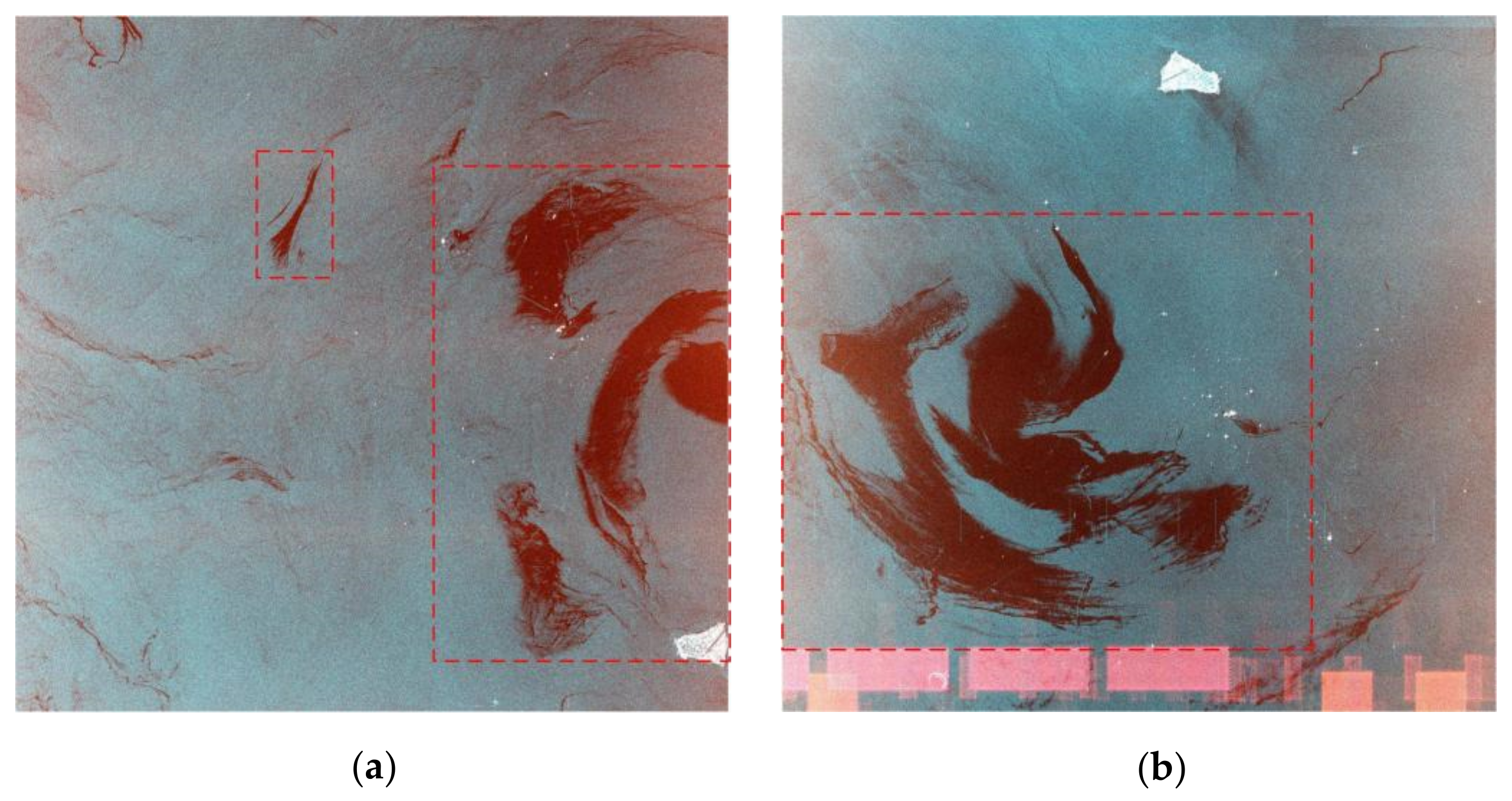
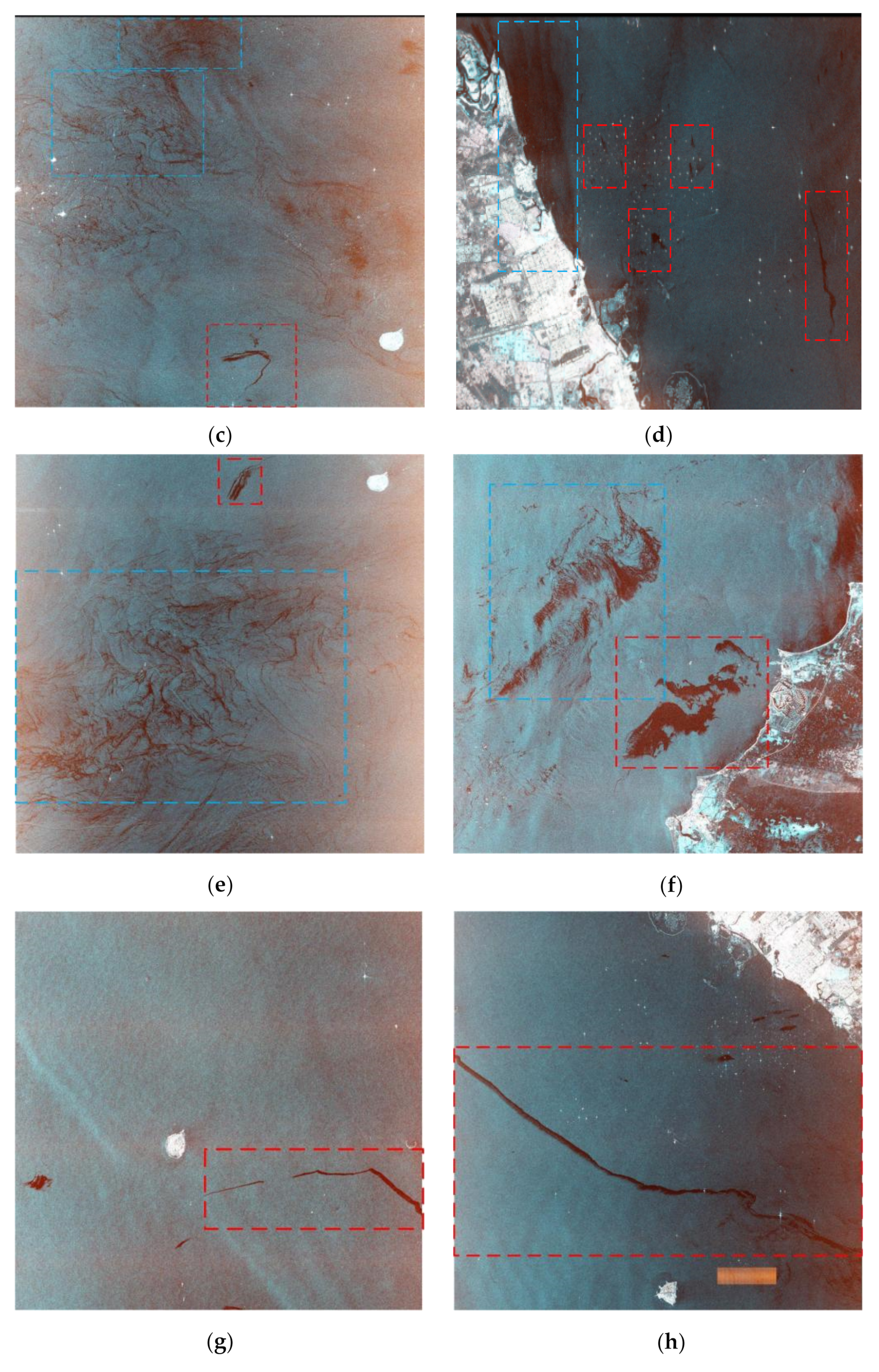
The SAR dataset was composed of Sentinel-1 dual-pol SAR data from the Persian Gulf region. The Persian Gulf is located between the Iranian Plateau and the Arabian Peninsula. Pollution is steadily increasing due to intensive oil production, serious tanker transportation, pipeline leakage, ship navigation, and maritime accidents in this area. According to Scanex [54], an average of 100,000–160,000 tons of oil and petroleum products flow into the Persian Gulf every year, and the degree of oil pollution is 47 times higher than the world average. In this section, eight VV/VH oil spill SAR data from Sentinel-1A in IW-SLC (interferometric wide swath, single-look complex) mode were selected for experiments. All images were numbered 1–8 in chronological order. Figure 6 presents the pseudo-color images of these eight images, where the dark spots within red dotted boxes are oil spill areas, while the blue dotted boxes represent look-alike areas. Oil spill areas were verified on the basis of in situ investigations and recorded by Scanex. Look-alike areas were present as dark spots on the images due to environmental or biological factors, as can be seen in Images 3–6 (see Figure 6c–f). The look-alike area marked in Image 6 (see Figure 6f) was recorded in previous studies [32,33]. Experts were invited to interpret the other unconfirmed dark spots in Images 3–5 (see Figure 6c–e). The dark spots in Figure 6d were identified as low-wind-speed areas, whereas Figure 6c,e represent biogenic oil films. According to the above information, we manually interpreted and labeled different areas on the image as the ground truth.

Table 2. Sentinel-1 data used in experiments.

Image Number	Date	ID	Stripes	Dark Spots Areas
1	8 March 2017	105080	IW1	Oil spill
2	11 March 2017	105355	IW3	Oil spill
3	18 April 2017	109672	IW3	Oil spill, look-alike
4	10 May 2017	112112	IW2	Oil spill, look-alike
5	5 June 2017	115163	IW3	Oil spill, look-alike
6	10 August 2017	122615	IW1	Oil spill, look-alike
7	10 October 2017	129633	IW1	Oil spill
8	10 October 2017	129633	IW2	Oil spill

shows the basic information of the images, with a central frequency of 5.405 × 10⁹ Hz. Each data point was marked manually, and the targets were divided into five classes: clean sea, oil spill, look-alike, land, and ship areas. Images were divided into small areas of 320 × 320 pixels for training and testing. In order to increase the number of samples, data enhancement operations such as rotation and resampling were carried out in some areas. The ratio of training to test data was about 4:1.

Table 3. Number of pixel samples of different classes.

	CS	OS	LA	LAND	SH
Training	3.028 × 107	1.095 × 107	8.110 × 106	4.313 × 106	5.601 × 104
Test	7.773 × 106	2.732 × 106	2.304 × 106	1.305 × 106	1.688 × 104

and

Table 4. Number of samples of different classes.

	CS	OS	LA	LAND	SH
Training	160	132	117	60	75
Test	40	34	30	15	19

show the number of samples belonging to each class.

In this paper, the mean intersection over union (MIoU) was taken as the main indicator to evaluate the classification effect. MIoU calculates the average value of the ratio of intersection and union of all classes, defined as

$$\mathrm{MIoU}=\frac{1}{k+1}{\displaystyle \sum _{i=0}^k\frac{P_{ii}}{{\displaystyle {\sum }_{i=0}^k{P}_{ij}}+{\displaystyle {\sum }_{i=0}^k{P}_{ji}}-P_{ii}}},$$

(17)

where k is the number of classes, i represents the real value, j represents the predicted value, and P_ij represents the prediction of i as j. In the semantic segmentation task, it is defined in the form of a confusion matrix as follows:

$$\mathrm{MIoU}=\frac{1}{k+1}{\displaystyle \sum _{i=0}^k\frac{TP}{FN+FP+TP}},$$

(18)

where TP means true positive, FN means false negative, and FP means false negative. For each individual category, the intersection over union (IoU) is calculated as

$$\mathrm{IoU}=\frac{TP}{FN+FP+TP}.$$

(19)

Other indices, such as the accuracy, precision, recall, and F1-score, are also used to indicate classification accuracy. They are defined as follows:

$$\mathrm{Accuracy}=\frac{TP+TN}{FN+FP+TP+TN},$$

(20)

$$\mathrm{Precision}=\frac{TP}{FP+TP},$$

(21)

$$\mathrm{Recall}=\frac{TP}{FN+TP},$$

(22)

$$\mathrm{F}1\_\mathrm{score}=\frac{2\times \mathrm{Precision}\times \mathrm{Recall}}{\mathrm{Precision}+\mathrm{Recall}}.$$

(23)

3.2. Polarization Decomposition and SLIC Superpixels

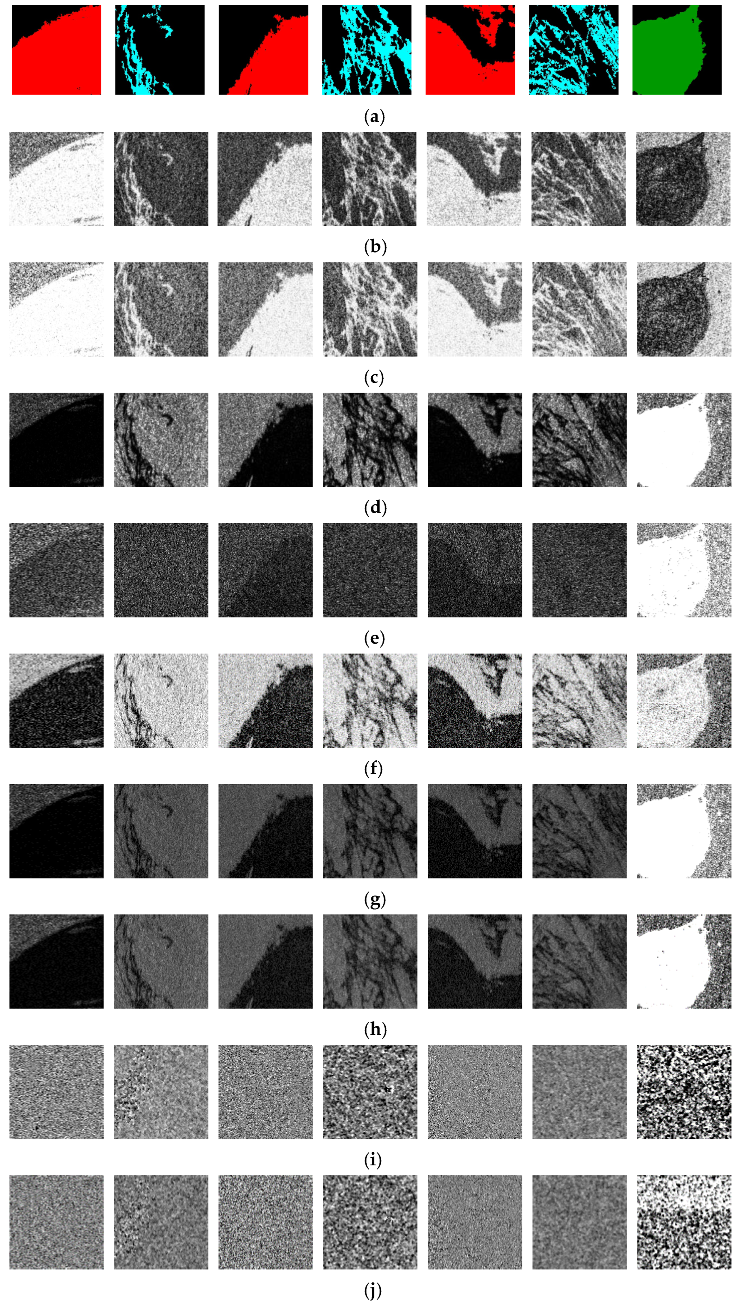
We applied polarization decomposition and SLIC superpixels to the SAR data according to the method introduced in Section 2. Two groups of polarimetric parameters were extracted: Group 1 (H/Alpha/λ₁/λ₂) parameters and Group 2 (Stokes) parameters.

Table 5. Average and variance of different polarized parameters.

		CS	OS	LA	LAND	SH
H	Average	0.5254	0.9719	0.9173	0.6380	0.6180
	Variance	0.0038	0.0006	0.0028	0.0341	0.0349
Alpha	Average	12.6749	40.3197	33.5511	20.0331	19.1461
	Variance	5.0410	14.5093	24.9643	51.0270	66.5614
λ1	Average	0.0104	0.0016	0.0042	0.2543	1.0049
	Variance	2.5366 × 10−6	7.6022 × 10−8	9.6723 × 10−7	4.1617	3.3318
λ2	Average	0.0014	0.0010	0.0021	0.0241	0.1156
	Variance	3.7614 × 10−8	1.6030 × 10−8	6.9204 × 10−8	0.0010	0.0247
Stokes-g0	Average	0.0118	0.0026	0.0063	0.2783	1.3210
	Variance	2.5764 × 10−6	1.1994 × 10−7	1.0547 × 10−6	4.1810	3.8715
Stokes-g1	Average	0.0090	0.0004	0.0019	0.2191	0.8730
	Variance	2.5728 × 10−6	9.3223 × 10−8	1.0947 × 10−6	4.0485	2.0367
Stokes-g2	Average	8.0368 × 10−5	−9.4482 × 10−6	−2.7806 × 10−5	−0.0175	−0.0458
	Variance	3.8482 × 10−7	4.3933 × 10−8	2.2210 × 10−7	0.0966	0.0161
Stokes-g3	Average	3.3683 × 10−5	2.5317 × 10−5	2.9162 × 10−5	0.0022	0.0889
	Variance	3.8098 × 10−7	4.3567 × 10−8	2.2311 × 10−7	0.0041	0.0066
Contrast	Average	0.7568	0.1306	0.2951	0.6223	0.6413
	Variance	0.0019	0.0095	0.0134	0.0221	0.0137

calculates the average and variance of different polarized parameters and different areas, reflecting their differences in numerical characteristics. As an example, Figure 7 presents the ground truth and several samples of extraction results from the dataset.

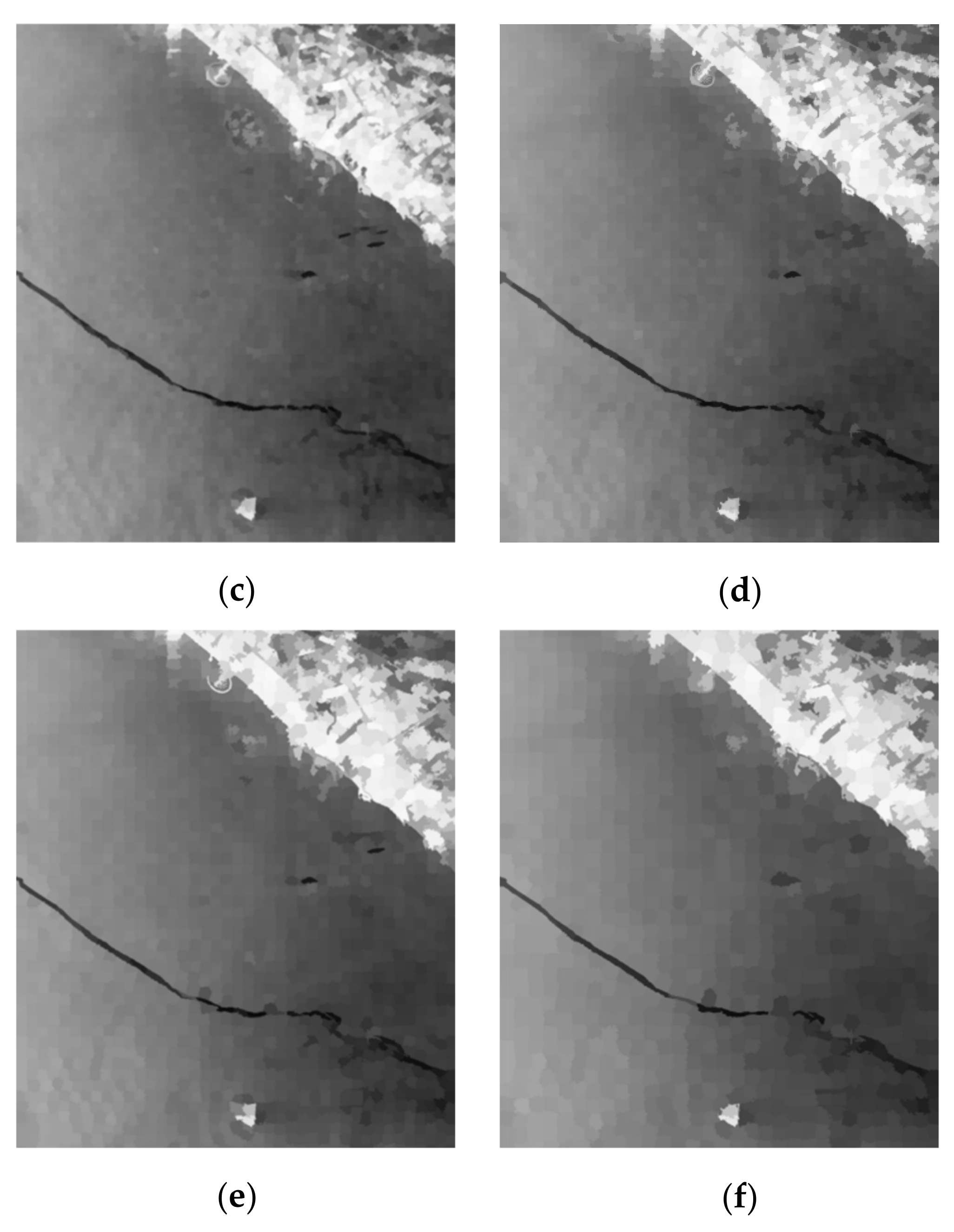
Superpixel numbers are among the key parameters used during superpixel calculation. They determine the size of the superpixel block. Bigger superpixel numbers indicate that each block contains fewer pixels. The influence of different superpixel number settings was tested as a function of the SLIC superpixels applied. Pixels in each superpixel block were categorized into six groups (50 × 50, 75 × 75, 100 × 100, 125 × 125, 150 × 150, and 200 × 200) to determine the suitable superpixel number for oil spill detection. All images were calculated according to different settings, and the average value of all pixels in each superpixel block was assigned to each point. Figure 8 presents the SLIC superpixel segmentation results of Image 8 as example.

SLIC superpixels with different settings were calculated for all eight images, and then input into the convolutional neural network model together with the polarized parameters for training and testing. The MIoU results are listed in

Table 6. MIoU of classification results based on polarimetric parameters with different SLIC superpixel numbers.

Superpixel Number	H/Alpha/λ1/λ2	Stokes
Without superpixel	70.6%	72.0%
50	75.9%	76.7%
75	77.0%	77.6%
100	77.3%	77.7%
125	77.2%	78.1%
150	75.5%	76.0%
200	75.2%	75.4%

.

The MIoU obtained using H/Alpha/λ₁/λ₂ parameters only was 70.6%, Stokes parameters achieved an MIoU of 72.0%. When the superpixel block contained 50 × 50, 75 × 75, 100 × 100, and 125 × 125 pixels, SLIC superpixels improved the classification accuracy. In the case of 150 × 150 and 200 × 200, the increase in MIoU was relatively low. Stokes parameters achieved the highest MIoU for the 125 × 125 setting (78.1%), whereas H/Alpha/λ₁/λ₂ parameters achieved an MIoU of 77.3% using the 100 × 100 superpixel setting.

Table 7. IoU values of oil spill detection with and without superpixels.

	H/Alpha/λ1/λ2		Stokes
	Without Superpixels	With 125 × 125 Superpixels	Without Superpixels	With 125 × 125 Superpixels
Clean sea	80.6%	87.0%	81.5%	88.3%
Oil spill	72.7%	78.5%	74.3%	78.5%
Look alike	65.3%	71.2%	68.1%	73.8%
Land	75.9%	81.3%	77.7%	82.4%
Ship	58.5%	66.9%	58.3%	67.7%

lists the IoU of the test results in different categories with and without superpixels, when the superpixels were set as 125 × 125.

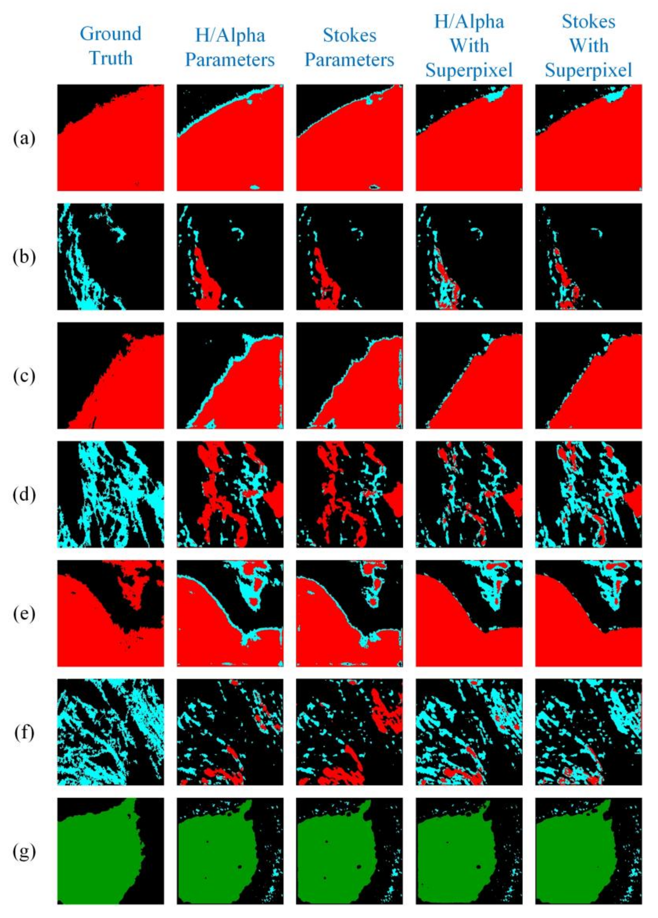
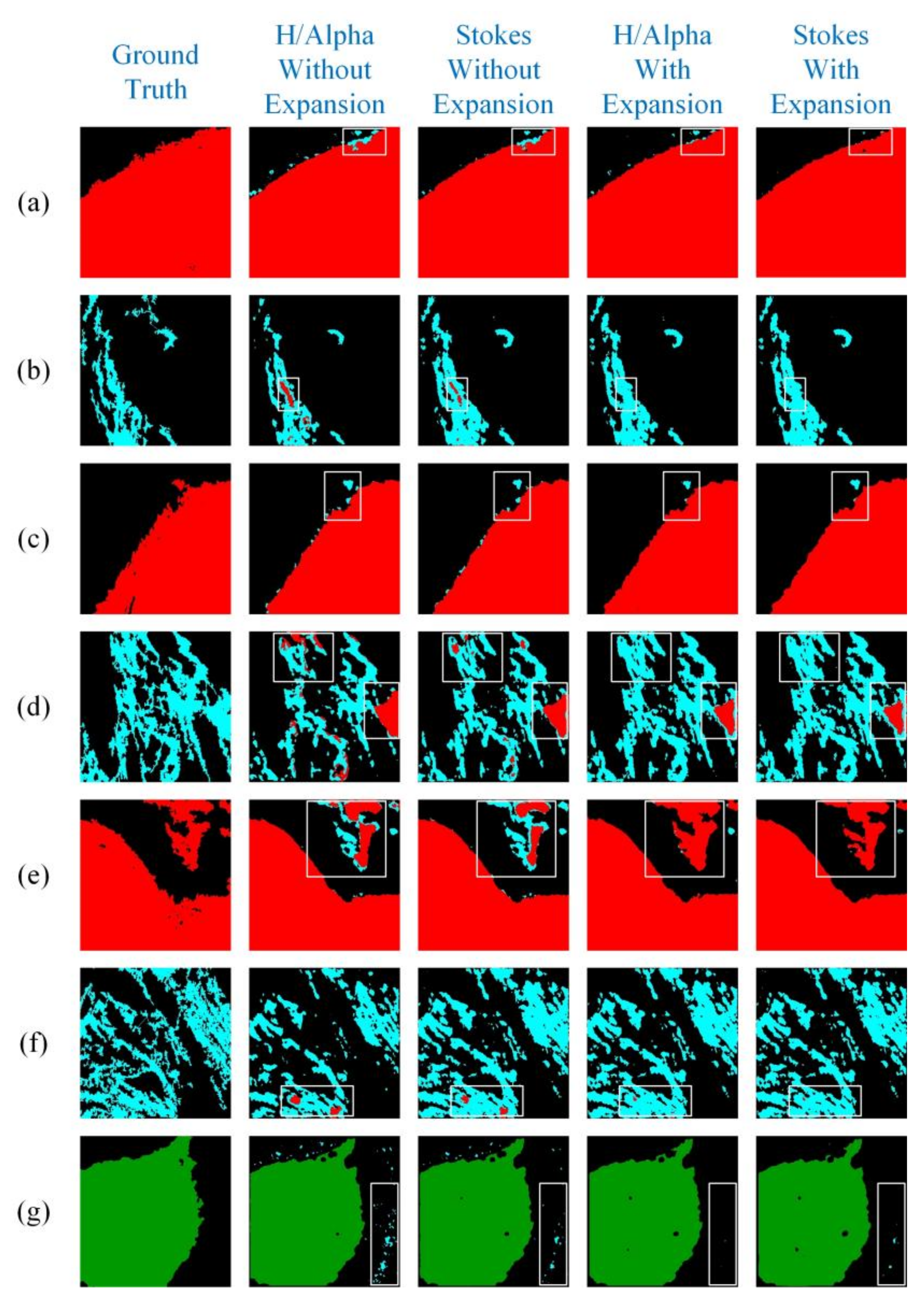
The IoU values of clean sea and land areas were higher, while those of look-alike areas were relatively lower. The IoU of oil spill areas increased to 78.5% in both groups using superpixels. This indicates that look alike areas could not be distinguished precisely despite superpixel segmentation being applied. Figure 9 presents the test results of several samples. When only polarized parameters were used, there was extensive misclassification of look alike and oil spill areas. This phenomenon was improved after introducing superpixels.

3.3. Oil Spill Detection Using Image Stretching Method

3.3.1. Image Stretching Based on Superpixels

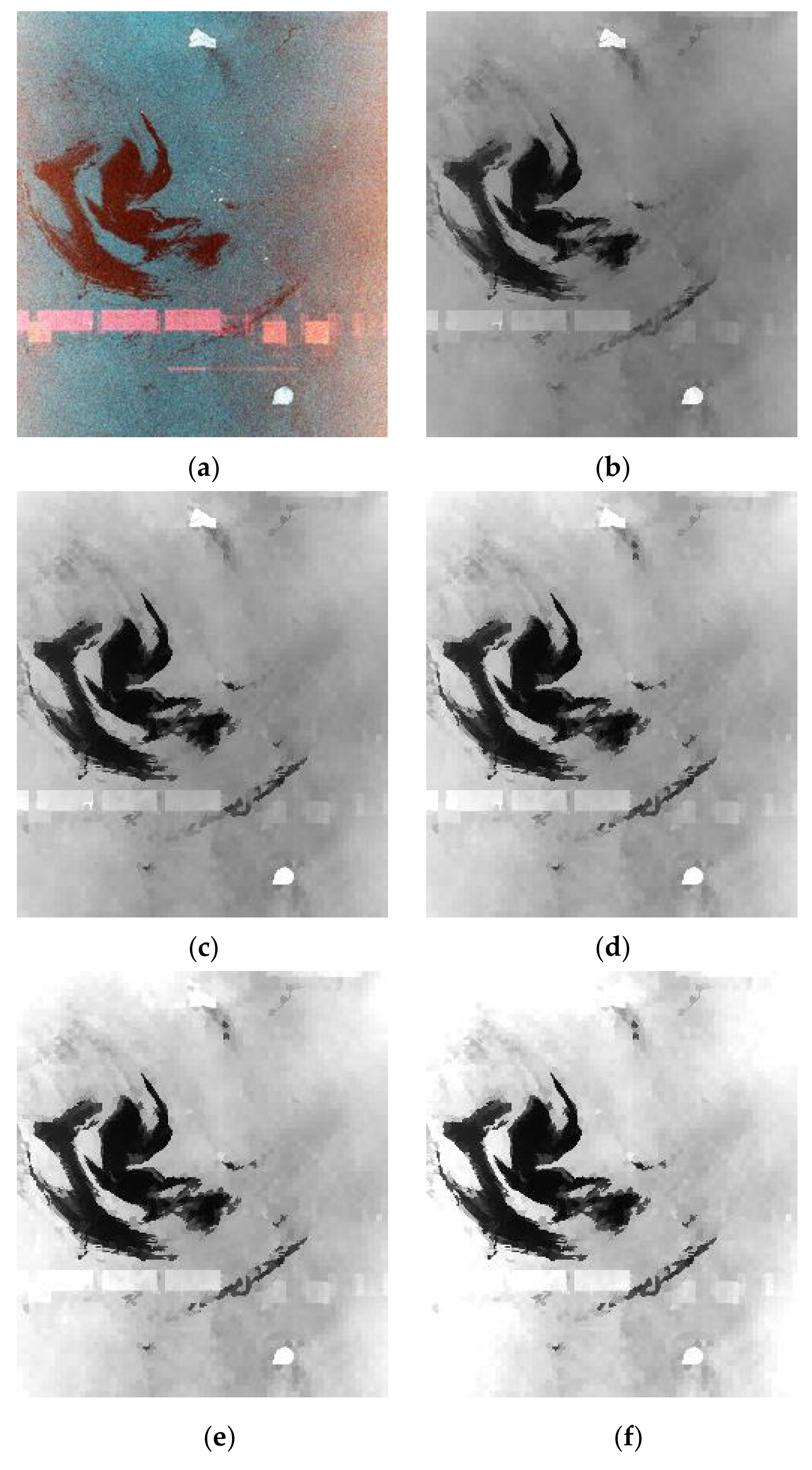
This section introduces the image stretching method based on SLIC superpixels for oil spill detection. Because the result of image stretching depends on the setting of the inhibition coefficient and expansion coefficient, the effects of these coefficients on oil spill detection was explored through experiments. For example, Figure 10 shows the calculation results of different expansion coefficients when the inhibition coefficient was kept constant at 1.05 in the oil spill area of Image 2. The stretched superpixel image and polarized parameters were combined as input into the neural network model for training and testing.

3.3.2. Oil Spill Detection as a Function of Inhibition Coefficient

We carried out further experiments while varying the inhibition coefficient. Firstly, we set the expansion coefficient to 1, and then we used inhibition coefficients of 1.05, 1.1, 1.15, and 1.2 to stretch the superpixel results. The image stretching results are presented in Figure 11. The results after image stretching and polarized parameters were used as input to the neural network model.

Table 8. MIoU value of different inhibition coefficients.

Inhibition Coefficient	None	1.05	1.1	1.15	1.2
H/Alpha/λ1/λ2	77.3%	77.8%	78.2%	78.8%	78.7%
Stokes	77.7%	78.6%	78.9%	79.5%	80.0%

lists the MIoU estimation results.

The results in Table 8 prove that the inhibition coefficient could improve the MIoU. When the inhibition coefficient was set as 1.15 or 1.2, the accuracy of oil spill detection was much better than for other settings. When the inhibition coefficient was set as 1.2 and the Stokes parameter was applied, the MIoU was the highest at 80%. H/Alpha parameters achieved MIoU values of 78.8% and 78.7% with inhibition coefficients set as 1.15 and 1.2, respectively. Subsequent experiments were conducted with the inhibition coefficient set as 1.2.

Table 9. Characteristics of polarized parameters in experiments.

	Clean Sea	Oil Spill	Look Alike	Land	Ship
H/Alpha/λ1/λ2	88.6%	79.8%	73.4%	83.0%	68.9%
Stokes	89.1%	80.9%	76.5%	84.4%	69.1%

presents the IoU value of each category when the inhibition coefficient was set as 1.2. Similar to when polarized parameters and superpixels were used, the accuracy was highest in the clean sea and land areas, slightly lower in the oil spill area, and lowest in the look alike and ship areas, as outlined in Table 9.

3.3.3. Oil Spill Detection as a Function of Expansion Coefficient

Experiments evaluating the effect of different expansion coefficients were carried out. We fixed the inhibition coefficient as 1.2 on the basis of the results from the previous section, and we varied the expansion coefficients as 1.2, 1.4, 1.6, and 1.8. Figure 12 illustrates the image stretching results for different expansion coefficients.

As the expansion coefficient was changed from 1.2 to 1.8, the characteristics of the oil spill area became more obvious. The stretching results and polarized parameters were combined as input into the neural network model for classification. The MIoU values with different expansion coefficients are listed in

Table 10. MIoU value of different inhibition coefficients.

Expansion Coefficient	None	1.2	1.4	1.6	1.8
H/Alpha/λ1/λ2	78.7%	80.0%	82.1%	84.5%	83.0%
Stokes	80.0%	81.7%	83.9%	85.4%	83.6%

.

When setting the expansion coefficient to 1.2, 1.4, 1.6, and 1.8, all MIoU values of the results were improved compared with using the inhibition coefficient only. The highest MIoU was achieved with the expansion coefficient set as 1.6, followed by 1.4, 1.8, and 1.2. The results for an expansion coefficient of 1.4 were very close to those for 1.8. The MIoU based on Stokes parameters reached 85.4%, while H/Alpha parameters achieved an MIoU of 84.5% with the expansion coefficient.

Table 11. IoU Values of polarized parameters with 125 × 125 superpixels and different expansion coefficients.

	Expansion	Clean Sea	Oil Spill	Look Alike	Land	Ship
H/Alpha/λ1/λ2	1.2	88.5%	84.7%	77.9%	84.4%	69.3%
	1.4	89.7%	88.1%	82.8%	86.8%	69.5%
	1.6	90.2%	89.3%	84.6%	88.7%	69.7%
	1.8	88.7%	89.1%	84.4%	87.2%	69.1%
Stokes	1.2	88.8%	85.3%	79.9%	86.6%	69.3%
	1.4	89.4%	88.8%	84.3%	88.5%	69.4%
	1.6	90.6%	90.1%	86.8%	89.0%	69.6%
	1.8	88.1%	89.2%	85.2%	87.0%	69.0%

and

Table 12. Indicators of Polarized parameters with 125 × 125 superpixels and different expansion coefficients.

	Expansion	Accuracy	Precision	Recall	F1-Score
H/Alpha/λ1/λ2	1.2	0.894	0.815	0.894	0.852
	1.4	0.921	0.835	0.907	0.870
	1.6	0.925	0.861	0.923	0.891
	1.8	0.920	0.836	0.905	0.869
Stokes	1.2	0.899	0.839	0.905	0.869
	1.4	0.926	0.847	0.919	0.881
	1.6	0.933	0.869	0.926	0.897
	1.8	0.928	0.844	0.914	0.878

list the IoU values of different classes and multiple indicators, which were used to evaluate the model with different expansion coefficients.

The use of expansion coefficients greatly improved the accuracy of oil spill and look-alike areas, with the highest IOU of the oil spill area reaching 88.6% with Stokes parameters. When the expansion coefficient was set as 1.2, 1.4, and 1.6, the accuracy was improved sequentially, with the rate of improvement being greatest for look-alike areas. When the expansion coefficient was increased from 1.6 to 1.8, the MIoU value of each region decreased slightly, while the oil spill region still maintained a high accuracy, as outlined in Table 11. When the expansion coefficient was set too high, the pixel values of land, clean sea, look alike, and ship areas on the superpixel segmentation images were over-enlarged could not be easily distinguished. An accuracy of 0.933 was achieved using Stokes parameters and a 1.6 expansion coefficient. The precision, recall, and F1-score were also highest at 0.869, 0.926, and 0.897, respectively. When setting the expansion coefficient as 1.6, the accuracy was highest at 0.925 using H/Alpha parameters. Figure 13 presents the test results using polarized parameters and the image stretching method. Compared with only applying the inhibition coefficient, the classification accuracy of look alike and oil spill area was further improved when the expansion coefficient was applied.

3.3.4. Validation of Image Stretching Method

This section evaluates the accuracy of the image stretching method proposed in this paper. Comparative experiments were carried out with and without image stretching. We chose samples from Image 1, Image 3, Image 5, Image 7, and Image 8 as the training set, while samples from Image 2, Image 4, and Image 6 were chosen as the test set. Stokes parameters were used in the experiments.

Table 13. IoU and MIoU values of validation experiments with and without image stretching.

	Image Stretching	Clean Sea	Oil Spill	Look Alike	Land	Ship	MIoU
Image 2	Without	86.2%	83.1%	-	84.3%	64.4%	79.5%
	With	88.7%	87.5%	-	88.4%	67.6%	83.1%
Image 4	Without	79.8%	76.6%	74.4%	77.7%	63.9%	74.5%
	With	84.3%	80.1%	79.9%	80.3%	67.0%	78.3%
Image 6	Without	84.1%	70.5%	65.7%	-	63.7%	71.0%
	With	89.1%	77.2%	73.3%	-	67.2%	76.7%
Average	Without	83.4%	76.7%	70.0%	81.0%	64.0%	75.0%
	With	87.4%	81.6%	76.6%	84.3%	67.3%	79.4%
Mean Square Deviation	Without	2.66%	5.19%	4.35%	3.30%	0.29%	3.49%
	With	2.24%	4.25%	3.30%	4.05%	0.25%	2.72%

‘-’ indicates no samples of this category on the current image.

shows the IoU and MIoU results of oil spill detection with and without image stretching. On the basis of the previous experiment, the inhibition coefficient and expansion coefficient were set as 1.2 and 1.6.

Table 13 shows that all the MIoU of the results of test images were higher with image stretching than without. The accuracy of each category was improved. The IoU of look-alike and oil spill areas improved by 6.6% and 4.9% on average, respectively. Oil spill achieved an MIoU of 81.6%, while clean sea and land areas could also be distinguished effectively. The average MIoU of the three images increased from 75.0% to 79.4%. Furthermore, with the exception of the land area, the mean square deviation of the IoU of different classes decreased, and the mean square deviation of MIoU values of different images also decreased from 3.49% to 2.72%. This proves that the image stretching method could significantly improve the accuracy of oil spill detection, as well as alleviate the inconsistency of accuracy caused by imaging differences.

3.4. Discussion

The experiments in this section focused on superpixel segmentation, the image stretching method, and polarized parameters. The number of superpixels determined the size of each superpixel block and affects the subsequent image stretching and classification results. The experimental results showed that, after 1:4 multi-look processing, the recognition accuracy was highest when each superpixel block contained 125 × 125 pixels, with the MIoU reaching 78.1% on the Stokes parameter. Image stretching involved setting the expansion and suppression coefficients and calculating the adaptive threshold to further process the segmentation results on the basis of superpixel segmentation. The purpose of this method was to divide the oil spill area and other areas in the image, so as to ensure the accurate classification of oil spill areas in the case of a large amount of data. When the expansion coefficient was set to 1.6 and the inhibition coefficient was set to 1.2, MIoU was increased to a maximum of 85.4%, achieving the highest accuracy. Subsequently, five images were used as the training set, and three images were used as the verification set. The experimental results showed that the average MIoU of different images increased from 75.0% to 79.4%, while the mean square deviation decreased from 3.49% to 2.72%, proving that this method could partially overcome the imaging differences and inconsistency of accuracy of different images while improving the accuracy.

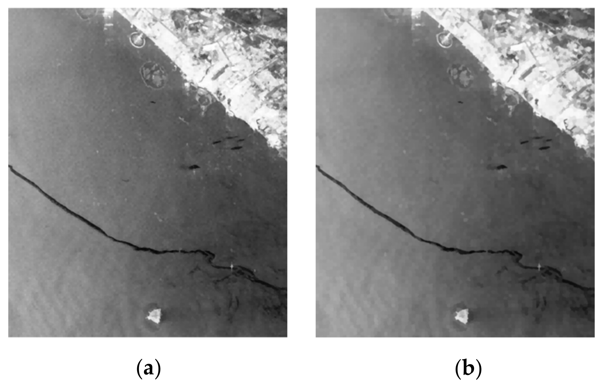
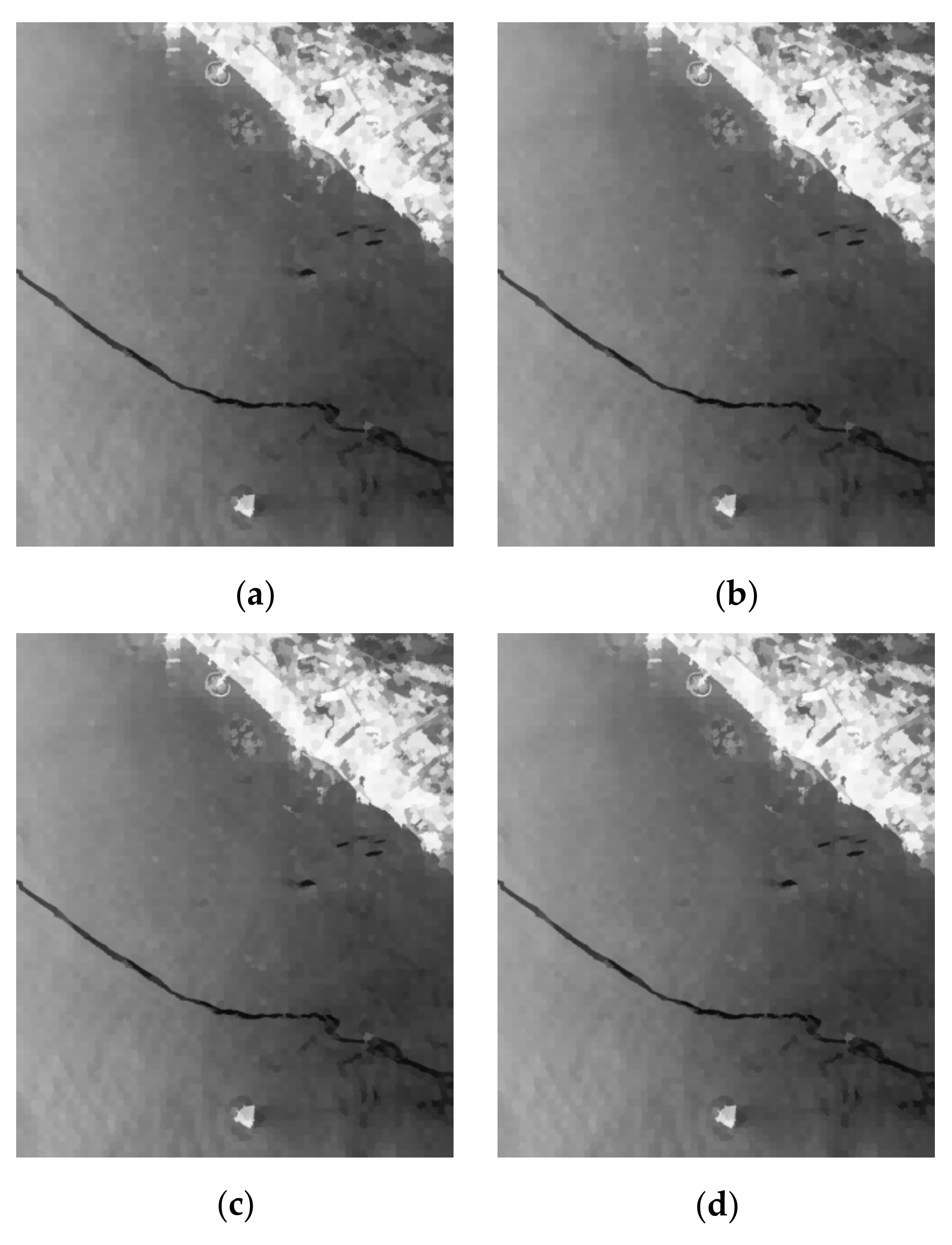
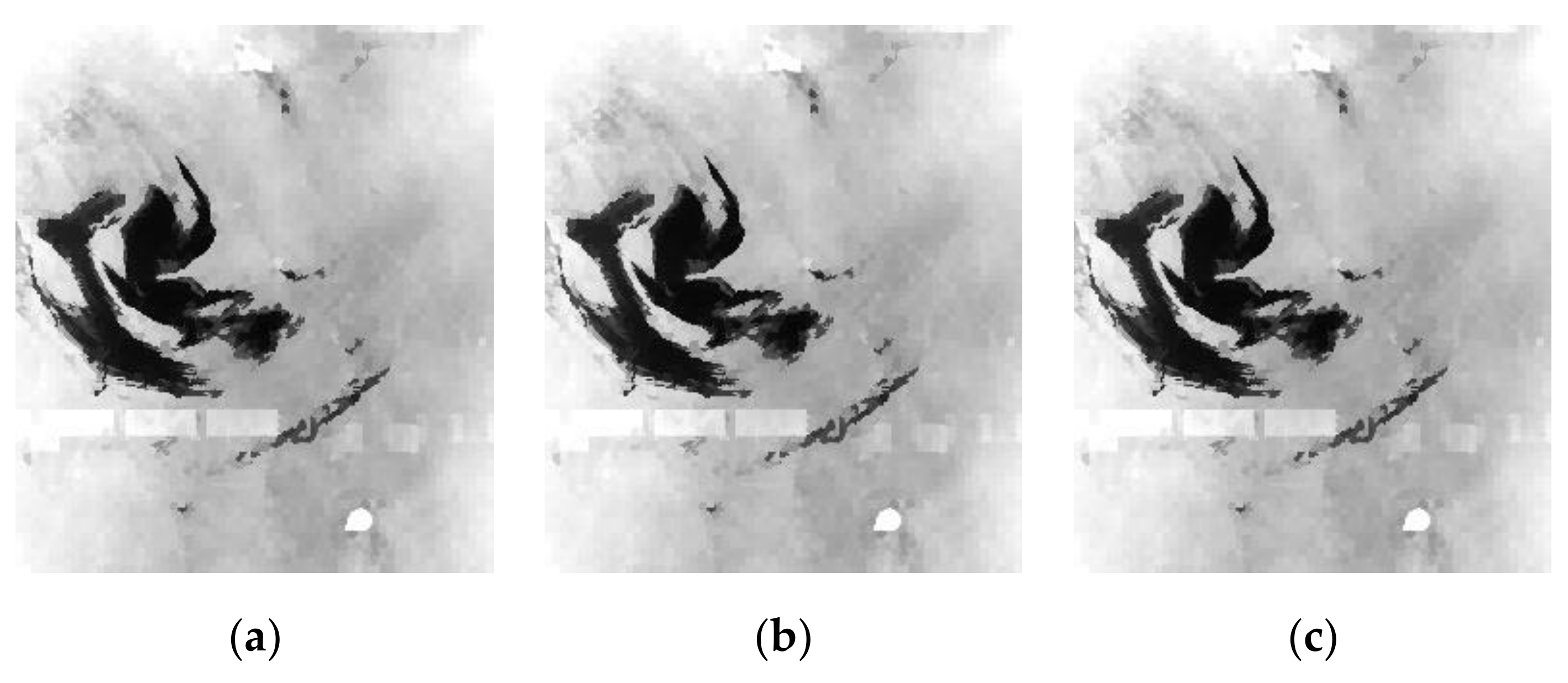
The image stretching method used in this paper depends on the threshold calculation of Equation (16). Its purpose is to characterize the boundary between oil spill dark spots and other areas, as well as retain the characteristics of the oil spill area through the inhibition coefficient and expansion coefficient, so as to overcome the distribution differences between different SAR data. Therefore, oil spill areas on different SAR images were classified within the same pixel distribution, while other similar regions were classified in another pixel distribution. In fact, it was found that the threshold is not an exact numerical value but usually an interval, and the threshold calculated by the formula fell into this interval. Taking Image 2 as example, Figure 14a,b show the processing results when the threshold was manually set to 0.67 and 0.73, respectively, while Figure 14c shows the processing results when the threshold was 0.69 according to the formula, and these three results were incredibly similar.

4. Conclusions

Polarized SAR data are widely used in oil spill detection. With the development of deep learning, more and more neural network models have been applied to oil spill detection and achieved good results. In this paper, we proposed an adaptive threshold calculation and image stretching method based on SLIC superpixels to overcome the influence of imaging differences between different SAR data, and we designed a semantic segmentation model to identify oil spill areas. Experiments were carried out on eight Sentinel-1 dual-pol SAR images. The experimental results showed that polarized parameters combined with SLIC superpixel segmentation could not effectively distinguish oil spill areas and similar areas, with the highest MIoU value only reaching 78.1%. After image stretching using the inhibition coefficient and expansion coefficient, the recognition accuracy of the two methods was greatly improved. The highest MIoU of the test set improved to 85.4%, while the accuracy and other indicators were also higher than those in other groups. Experiments on single images showed that this method partly overcame the imaging difference and inconsistent accuracy of Sentinel-1 dual-pol SAR data.

There were still some limitations of our current research. The optimal superpixel number used in the SLIC superpixel model depends on actual situations of the study site. This paper only discussed the impact of superpixel number on the current dataset, which may need to be adjusted according to the specific situation. Thus, future research can focus on adaptive optimization of the superpixel number. The current threshold of image stretching is set by experiments, and more data experiments and theoretical analyses are required. Future research can focus on expanding the data experiments and the adaptive threshold calculation, including numerical fitting and machine learning. From the perspective of the neural network, further research can be conducted on the improvement of the model structure explored in this paper. Introducing an appropriate attention mechanism is one option for enhancing the extraction and utilization of texture information in oil spill areas.

References

1. Liu, Y.; MacFadyen, A.; Ji, Z.G.; Weisberg, R.H. Monitoring and Modeling the Deepwater Horizon Oil Spill: A Record-Breaking Enterprise. Geophys. Monogr. Ser. 2011, 195, 205–215. [Google Scholar]
2. Alpers, W.; Holt, B.; Zeng, K. Oil spill detection by imaging radars: Challenges and pitfalls. Remote Sens. Environ. 2017, 201, 133–147. [Google Scholar] [CrossRef]
3. Merv, F.; Carl, E.B. A Review of Oil Spill Remote Sensing. Sensors 2017, 18, 91–108. [Google Scholar]
4. Solberg, A.H.S.; Storvik, G.; Solberg, R.; Volden, E. Automatic detection of oil spills in ERS SAR images. IEEE Trans. Geosci. Remote Sens. 1999, 37, 1916–1924. [Google Scholar] [CrossRef]
5. Solberg, A.H.S.; Brekke, C.; Husoy, P.O. Oil Spill Detection in Radarsat and Envisat SAR Images. IEEE Trans. Geosci. Remote Sens. 2007, 45, 746–755. [Google Scholar] [CrossRef]
6. Garcia-Pineda, O.; MacDonald, I.R.; Li, X.; Jackson, C.R.; Pichel, W.G. Oil Spill Mapping and Measurement in the Gulf of Mexico With Textural Classifier Neural Network Algorithm (TCNNA). IEEE J. Sel. Top. Appl. Earth Obs. Remote Sens. 2013, 6, 2517–2525. [Google Scholar] [CrossRef]
7. Cheng, Y.; Liu, B.; Li, X.; Nunziata, F.; Xu, Q. Monitoring of Oil Spill Trajectories With COSMO-SkyMed X-Band SAR Images and Model Simulation. IEEE J. Sel. Top. Appl. Earth Obs. Remote Sens. 2014, 7, 2895–2901. [Google Scholar] [CrossRef]
8. Fustes, D.; Cantorna, D.; Dafonte, C.; Arcay, B.; Iglesias, A.; Manteiga, M. A cloud-integrated web platform for marine monitoring using GIS and remote sensing. Application to oil spill detection through SAR images. Future Gener. Comput. Syst. 2014, 34, 155–160. [Google Scholar] [CrossRef]
9. Trivero, P.; Adamo, M.; Biamino, W.; Borasi, M.; Cavagnero, M.; De Carolis, G.; Di Matteo, L.; Fontebasso, F.; Nirchio, F.; Tataranni, F. Automatic oil slick detection from sar images: Results and improvements in the framework of the PRIMI pilot project. Deep Sea Res. Part II Top. Stud. Oceanogr. 2016, 133, 146–158. [Google Scholar] [CrossRef]
10. Ajadi Olaniyi, A. Unsupervised Multi-Scale Change Detection from SAR Imagery for Monitoring Natural and Anthropogenic Disasters. Ph.D. Thesis, University of Alaska Fairbanks, Fairbanks, AK, USA, 2017. [Google Scholar]
11. Ajadi, O.; Meyer, F.J.; Tello, M.; Ruello, G. Oil Spill Detection in Synthetic Aperture Radar Images Using Lipschitz-Regularity and Multiscale Techniques. IEEE J. Sel. Top. Appl. Earth Obs. Remote Sens. 2018, 11, 2389–2405. [Google Scholar] [CrossRef]
12. Cloude, S.R. Group theory and polarization algebra. Optic 1986, 75, 26–36. [Google Scholar]
13. Cloude, S.; Pottier, E. An entropy based classification scheme for land applications of polarimetric SAR. IEEE Trans. Geosci. Remote Sens. 1997, 35, 68–78. [Google Scholar] [CrossRef]
14. Allain, S.; Ferro-Famil, L.; Pottier, E. Two novel surface model based inversion algorithms using multi-frequency PolSAR data. In Proceedings of the 2004 IEEE International Geoscience and Remote Sensing Symposium, Anchorage, AK, USA, 20–24 September 2004. [Google Scholar]
15. Yamaguchi, Y.; Moriyama, T.; Ishido, M.; Yamada, H. Four-component scattering model for polarimetric SAR image decomposition. IEEE Trans. Geosci. Remote Sens. 2005, 43, 1699–1706. [Google Scholar] [CrossRef]
16. Skrunes, S.; Brekke, C.; Eltoft, T. Characterization of Marine Surface Slicks by Radarsat-2 Multipolarization Features. IEEE Trans. Geosci. Remote Sens. 2014, 52, 5302–5319. [Google Scholar] [CrossRef]
17. Li, H.; Perrie, W.; He, Y.; Wu, J.; Luo, X. Analysis of the Polarimetric SAR Scattering Properties of Oil-Covered Waters. IEEE J. Sel. Top. Appl. Earth Obs. Remote Sens. 2015, 8, 3751–3759. [Google Scholar] [CrossRef]
18. Salberg, A.-B.; Rudjord, O.; Solberg, A.H.S. Oil Spill Detection in Hybrid-Polarimetric SAR Images. IEEE Trans. Geosci. Remote Sens. 2014, 52, 6521–6533. [Google Scholar] [CrossRef]
19. Salberg, A.-B.; Larsen, S.O. Classification of Ocean Surface Slicks in Simulated Hybrid-Polarimetric SAR Data. IEEE Trans. Geosci. Remote Sens. 2018, 56, 7062–7073. [Google Scholar] [CrossRef]
20. Dmitry, I.; Camilla, B.; Stine, S.; Andrei, I.; Nataliya, K. Mineral Oil Slicks Identification Using Dual Co-polarized Radarsat-2 and TerraSAR-X SAR Imagery. Remote Sens. 2020, 12, 1061–1086. [Google Scholar]
21. Espeseth, M.M.; Brekke, C.; Jones, C.E.; Holt, B.; Freeman, A. The Impact of System Noise in Polarimetric SAR Imagery on Oil Spill Observations. IEEE Trans. Geosci. Remote Sens. 2020, 58, 4194–4214. [Google Scholar] [CrossRef]
22. Guannan, L.; Ying, L.; Yongchao, H.; Xiang, W.; Lin, W. Marine Oil Slick Detection Using Improved Polarimetric Feature Parameters Based on Polarimetric Synthetic Aperture RadAar Data. Remote Sens. 2021, 13, 1607–1629. [Google Scholar]
23. Long, J.; Shelhamer, E.; Darrell, T. Fully Convolutional Networks for Semantic Segmentation. IEEE Trans. Pattern Anal. Mach. Intell. 2015, 39, 640–651. [Google Scholar]
24. Ronneberger, O.; Fischer, P.; Brox, T. U-Net: Convolutional Networks for Biomedical Image Segmentation. In Proceedings of the International Conference on Medical Image Computing and Computer-Assisted Intervention, Munich, Germany, 5–9 October 2015. [Google Scholar]
25. Zhao, H.; Shi, J.; Qi, X.; Wang, X.; Jia, J. Pyramid Scene Parsing Network. In Proceedings of the 2017 IEEE Conference on Computer Vision and Pattern Recognition (CVPR), Honolulu, HI, USA, 21–26 July 2017; pp. 6230–6239. [Google Scholar]
26. Chen, L.C.; Zhu, Y.; Papandreou, G.; Schroff, F.; Adam, H. Encoder-Decoder with Atrous Separable Convolution for Semantic Image Segmentation. In Proceedings of the European Conference on Computer Vision, Munich, Germany, 8–14 September 2018. [Google Scholar]
27. Liu, C.; Chen, L.C.; Schroff, F.; Adam, H.; Hua, W.; Yuille, A.L.; Fei-Fei, L. Auto-DeepLab: Hierarchical Neural Architecture Search for Semantic Image Segmentation. In Proceedings of the 2019 IEEE/CVF Conference on Computer Vision and Pattern Recognition (CVPR), Long Beach, CA, USA, 15–20 June 2019; pp. 82–92. [Google Scholar]
28. Yuan, Y.; Chen, X.; Wang, J. Object-Contextual Representations for Semantic Segmentation. In Proceedings of the European Conference on Computer Vision, Munich, Germany, 8–14 September 2018. [Google Scholar]
29. Kan, Z.; Wang, Y. A Deep Convolutional Neural Network for Oil Spill Detection from Spaceborne SAR Images. Remote Sens. 2020, 6, 1015–1037. [Google Scholar]
30. Yu, X.; Zhang, H.; Luo, C.; Qi, H.; Ren, P. Oil Spill Segmentation via Adversarial f-Divergence Learning. IEEE Trans. Geosci. Remote Sens. 2018, 56, 4973–4988. [Google Scholar] [CrossRef]
31. Filippo Maria, B.; Espeseth Martine, M.; Borch, N. Large-Scale Detection and Categorization of Oil Spills from SAR Images with Deep Learning. Remote Sens. 2020, 12, 2260–2286. [Google Scholar]
32. Zhang, J.; Feng, H.; Luo, Q.; Li, Y.; Li, J. Oil spill detection in quad-polarimetric sar images using an advanced convolutional neural network based on superpixel model. Remote Sens. 2020, 12, 944. [Google Scholar] [CrossRef]
33. Li, Y.; Lyu, X.; Frery, A.C.; Ren, P. Oil Spill Detection with Multiscale Conditional Adversarial Networks with Small-Data Training. Remote Sens. 2021, 13, 2378. [Google Scholar] [CrossRef]
34. Seydi, S.T.; Hasanlou, M.; Amani, M.; Huang, W. Oil Spill Detection Based on Multiscale Multidimensional Residual CNN for Optical Remote Sensing Imagery. IEEE J. Sel. Top. Appl. Earth Obs. Remote Sens. 2021, 14, 10941–10952. [Google Scholar] [CrossRef]
35. Zhu, Q.; Zhang, Y.; Li, Z.; Yan, X.; Guan, Q.; Zhong, Y.; Zhang, L.; Li, D. Oil Spill Contextual and Boundary-Supervised Detection Network Based on Marine SAR Images. IEEE Trans. Geosci. Remote Sens. 2022, 60, 5213910. [Google Scholar] [CrossRef]
36. Akhmadiya, A.; Nabiyev, N.; Moldamurat, K.; Dyussekeyev, K.; Atanov, S. Use of Sentinel-1 Dual Polarization Multi-Temporal Data with Gray Level Co-Occurrence Matrix Textural Parameters for Building Damage Assessment. Pattern Recognit. Image Anal. 2021, 31, 240–250. [Google Scholar] [CrossRef]
37. Liu, J.; Hu, J.; Li, Z.; Wu, L.; Jiang, W.; Feng, G.; Zhu, J. Complete three-dimensional coseismic displacements due to the 2021 Maduo earthquake in Qinghai Province, China from Sentinel-1 and ALOS-2 SAR images. Sci. China Earth Sci. 2022, 65, 687–697. [Google Scholar] [CrossRef]
38. Luo, Q.; Perissin, D.; Zhang, Y.; Youliang, J. L- and X-Band Multi-Temporal InSAR Analysis of Tianjin Subsidence. Remote Sens. 2014, 6, 7933–7951. [Google Scholar] [CrossRef]
39. Luo, Q.; Zhou, G.; Perissin, D. Monitoring of Subsidence along Jingjin Inter-city Railway by High resolution TSX MT-INSAR analysis. Remote Sens. 2017, 9, 717. [Google Scholar] [CrossRef]
40. Xiao, R.; Jiang, M.; Li, Z.; He, X. New insights into the 2020 Sardoba dam failure in Uzbekistan from Earth observation. Int. J. Appl. Earth Obs. Geoinf. 2022, 107, 102705. [Google Scholar] [CrossRef]
41. Setiani, P.; Ramdani, F. Oil spill mapping using multi-sensor Sentinel data in Balikpapan Bay, Indonesia. In Proceedings of the 2018 4th International Symposium on Geoinformatics (ISyG), Malang, Indonesia, 10–12 November 2018. [Google Scholar]
42. Rajendran, S.; Vethamony, P.; Sadooni, F.N.; Al-Kuwari, A.S.; Nasir, S. Detection of Wakashio oil spill off Mauritius using Sentinel-1 and 2 data: Capability of sensors, image transformation methods and mapping. Environ. Pollut. 2021, 274, 116618–116628. [Google Scholar] [CrossRef]
43. Saima, N.; Muhammad, I.; Irfan, M.; Mona, A. Marine oil spill detection using Synthetic Aperture Radar over Indian Ocean. Mar. Pollut. Bull. 2021, 162, 111921. [Google Scholar]
44. Diego, C.; Carlos, D.; Alfonso, I.; Arcay, B. Oil spill segmentation in SAR images using convolutional neural networks. A comparative analysis with clustering and logistic regression algorithms. Appl. Soft Comput. 2019, 84, 105716. [Google Scholar]
45. Chaturvedi, S.K.; Banerjee, S.; Lele, S. An assessment of oil spill detection using Sentinel 1 SAR-C images. J. Ocean. Eng. Sci. 2020, 5, 116–135. [Google Scholar] [CrossRef]
46. Valeria, C.; Andrea, B.; Ferdinando, N.; Maurizio, M. A Sensitivity Analysis on the Spectral Signatures of Low-Backscattering Sea Areas in Sentinel-1 SAR Images. Remote Sens. 2021, 13, 1183–1199. [Google Scholar]
47. Marios, K.; Georgios, O.; Konstantinos, I.; Konstantinos, A.; Stefanos, V.; Ioannis, K. Oil Spill Identification from Satellite Images Using Deep Neural Networks. Remote Sens. 2019, 11, 1762–1783. [Google Scholar]
48. Ma, X.; Xu, J.; Wu, P.; Kong, P. Oil Spill Detection Based on Deep Convolutional Neural Networks Using Polarimetric Scattering Information From Sentinel-1 SAR Images. IEEE Trans. Geosci. Remote Sens. 2022, 60, 4204713. [Google Scholar] [CrossRef]
49. Dong, Y.; Liu, Y.; Hu, C.; MacDonald, I.R.; Lu, Y. Chronic oiling in global oceans. Science 2022, 376, 1300–1304. [Google Scholar] [CrossRef]
50. Shang, F.; Hirose, A. Averaged Stokes Vector Based Polarimetric SAR Data Interpretation. IEEE Trans. Geosci. Remote Sens. 2015, 53, 4536–4547. [Google Scholar] [CrossRef]
51. Raney, R.K. Dual-polarized SAR and Stokes parameters. IEEE Geosci. Remote Sens. Lett. 2006, 3, 317–319. [Google Scholar] [CrossRef]
52. He, K.; Zhang, X.; Ren, S.; Sun, J. Deep Residual Learning for Image Recognition. In Proceedings of the 2016 IEEE Conference on Computer Vision and Pattern Recognition (CVPR), Las Vegas, NV, USA, 27–30 June 2016; pp. 770–778. [Google Scholar]
53. Achanta, R.; Shaji, A.; Smith, K.; Lucchi, A.; Fua, P.; Süsstrunk, S. SLIC Superpixels Compared to State-of-the-Art Superpixel Methods. IEEE Trans. Pattern Anal. Mach. Intell. 2012, 34, 2274–2282. [Google Scholar] [CrossRef]
54. ScanEx. Satellite Monitoring of Oil Pollution in the Persian Gulf. Available online: https://www.scanex.ru/en/company/news/satellite-monitoring-of-oil-pollution-in-the-persian-gulf/ (accessed on 29 January 2018).
Figure 1. Overall flowchart of the proposed oil spill detection algorithm.
Remotesensing 14 03900 g001
Figure 2. Polarization decomposition parameters: H/Alpha decomposition and Stokes parameters.
Remotesensing 14 03900 g002
Figure 3. Detailed structure of Resblock.
Remotesensing 14 03900 g003
Figure 4. Structure diagram of neural network model.
Remotesensing 14 03900 g004
Figure 5. Structure of feature extraction module and data input/output segments: (a) feature extraction module; (b) data input segment; (c) data output segment.
Remotesensing 14 03900 g005aRemotesensing 14 03900 g005b
Figure 6. Pseudo-color images. The dark spots within red dotted boxes represent oil spill area, while blue dotted boxes represent look-alike areas: (a) Image 1, (b) Image 2, (c) Image 3, (d) Image 4, (e) Image 5, (f) Image 6, (g) Image 7, and (h) Image 8.
Remotesensing 14 03900 g006aRemotesensing 14 03900 g006b
Figure 7. The ground truth and polarized parameter extraction results of the samples used in the experiment. In the ground truth, red represents oil spill, blue represents look-alike, and green represents land areas: (a) ground truth, (b) Alpha, (c) H, (d) λ1, (e) λ2, (f) Stokes-contrast, (g) Stokes-g0, (h) Stokes-g1, (i) Stokes-g2, and (j) Stokes-g3.
Remotesensing 14 03900 g007
Figure 8. SLIC superpixel results of Image 8 using different superpixel number settings: (a) 50 × 50, (b) 75 × 75, (c) 100 × 100, (d) 125 × 125, (e) 150 × 150, and (f) 200 × 200.
Remotesensing 14 03900 g008aRemotesensing 14 03900 g008b
Figure 9. Classification results of some typical samples using polarized parameters and SLIC superpixels. Red represents oil spill, blue represents look alike, while green represents land areas. (a) oil spill, (b) look alike, (c) oil spill, (d) look alike, (e) oil spill, (f) look alike, (g) land.
Remotesensing 14 03900 g009
Figure 10. Image stretching result with different expansion coefficients: (a) original pseudo-color image, (b) SLIC superpixel, (c) SLIC superpixel with 1.2 expansion coefficient, (d) SLIC superpixel with 1.4 expansion coefficient, (e) SLIC superpixel with 1.6 expansion coefficient, and (f) SLIC superpixel with 1.8 expansion coefficient.
Remotesensing 14 03900 g010
Figure 11. Image stretching results using different inhibition coefficients: (a) 1.05, (b) 1.1, (c) 1.15, and (d) 1.2.
Remotesensing 14 03900 g011
Figure 12. Image stretching results using different expansion coefficients: (a) 1.2, (b) 1.4, (c) 1.6, and (d) 1.8.
Remotesensing 14 03900 g012
Figure 13. Classification results of several samples using polarized parameters and image stretching. Red represents oil spill, blue represents look alike, while green represents land areas. (a) oil spill, (b) look alike, (c) oil spill, (d) look alike, (e) oil spill, (f) look alike, (g) land.
Remotesensing 14 03900 g013
Figure 14. Image stretching results with different thresholds: (a) 0.67, (b) 0.73, and (c) 0.69.
Remotesensing 14 03900 g014