Article

A Multivariate Drought Index for Seasonal Agriculture Drought Classification in Semiarid Regions

School of Environment and Society, Tokyo Institute of Technology, Yokohama 226-8503, Japan
*
Author to whom correspondence should be addressed.
Remote Sens. 2022, 14(16), 3891; https://doi.org/10.3390/rs14163891
Submission received: 5 July 2022 / Revised: 6 August 2022 / Accepted: 8 August 2022 / Published: 11 August 2022
(This article belongs to the Special Issue Remote Sensing for Advancing Nature-Based Climate Solutions)

Abstract

:
Drought assessment in any region primarily hinges on precipitation deficiency, which is subsequently propagated to various components and sectors, leading to different drought types. In countries such as India, an intricate relationship between various governing factors, drought types, and their quantification methodologies make it elusive to timely initiate government relief measures. This also prevents comprehensive inclusion of the integrated effect of the principal drivers of drought, resulting in ambiguous categorization of severity, where groundwater storage variability is often neglected despite its significant role in irrigation. Here, we developed a multivariate Joint Drought Index (JDI) combining satellite and model-based standardized indices of precipitation and evapotranspiration (SPEI), soil moisture (SSI), groundwater (SGI), and surface runoff (SRI) with different temporal scales by employing two robust methods, principal component analysis (PCA) and Gaussian copula, and applied the index to highly drought-prone Marathwada region from central India. Our novel approach of using different scale combinations of integrated indices for two primary seasons (Kharif and Rabi) provides more realistic drought intensities than multiple univariate indices, by incorporating the response from each index, representing the seasonal drought conditions corroborating with the seasonal crop yields. JDI, with both methods, successfully identified two major drought events in 2015 and 2018, while effectively capturing the groundwater drought. Moreover, despite the high correlation between JDI using PCA and copula, we observed a significant difference in the intensities reported by these methods, where copula detected exceptional drought conditions more frequently than PCA. JDI effectively detected the onset, duration, and termination of drought, where the improved accuracy of drought detection can play a critical role in policy formation and socioeconomic security of the related stakeholders. Seasonal agriculture drought categorization for holistic quantification of drought conditions as presented in this study should provide broad methodological implications on drought monitoring and mitigation measures, especially for agriculture-dominated regions in semiarid climates.

Graphical Abstract

1. Introduction

Droughts are spatially extensive water extreme events with multidimensional impacts that have incurred a huge cost in related damages in the past century, with multifold devastation in worldwide economies [1,2,3]. This widespread water scarcity is increasing year by year, pertaining to population growth, agricultural expansion, and growing water demands for energy and industrial sectors, exaggerating the pronounced and multifarious impacts of droughts [4]. The droughts in specific areas of the world are projected to increase in severity as well as intensity in the near future, subject to climate shifts towards warmer temperatures, decrease in precipitation, and an increase in evapotranspiration [5,6,7]. On the backdrop of progressively detrimental effects of climate change, drought assessment, especially in countries such as India, is of paramount importance, considering its exclusively agrarian economy. Despite being a global agriculture powerhouse, about 68% of cropped area in India is highly vulnerable to drought, with 33% being chronically drought-prone [8], where compounding effects of droughts have caused an immense loss in terms of agriculture failures, food insecurities, widespread distress issues, and even farmer suicides [9,10,11,12,13]. The societal impacts of droughts are more persistent and prolonged than other natural calamities, which see great migrations, water scarcity, political instabilities, livestock issues, women, and health-related problems, along with intensifying agricultural crises [14]. India has also faced miserable famines owing to droughts in the past century [15]. Moreover, unsustainable extraction of groundwater, which is the primary source of irrigation in India, is expected to further magnify the agricultural stress under the threat of climate change, disturbing the routine agricultural activities to a great extent [9,16,17]. Considering these profound social, economic, and hydro-climatological impacts of the droughts on multiple aspects of life, comprehensive and efficient drought monitoring and mitigation, along with a subsequent assessment of drought severity, is imperative to maintain the socioeconomic security in India.
Unfortunately, a comprehensive universal definition of drought is difficult to formulate, considering its diverse range of drivers and impacts. This has led to the classification of drought in multiple domains (meteorological, agricultural, hydrological, groundwater, social, etc. [18]), hindering the inclusion of the integrated effect of various critical parameters and thorough determination of drought characteristics (such as onset, end, and duration) using a single indicator. The conventional approach of drought quantification is mainly dependent on ground-based hydro-meteorological data. Multiple indices have been developed to date for drought monitoring, including traditional ones, such as Palmer Drought Severity Index [19], Standardized Precipitation Index (SPI; [20]), Standardized Precipitation, Evapotranspiration Index (SPEI, [21]), and remote-sensing-based indices, such as Normalized Difference Vegetation Index (NDVI; [22,23]), Vegetation Health Index (VHI; [24]), Vegetation Condition Index (VCI; [25]), Evaporative Stress Index (ESI; [26,27]), and many more ([28]). The accuracy of these traditional approaches is mainly constrained by the data gaps, inadequate monitoring network, and data unavailability in required spatiotemporal scales. Remote-sensing-based indices, on the other hand, provide fine-resolution, near real-time, and consistent data observations, which are advantageous over traditional methods and provide unique drought monitoring opportunities [18]. However, all these indices rely on a single surface or subsurface water storage and vegetation character irrespective of the combined effect from other hydro-climatological parameters, thus failing to capture the integrated water deficit effect, which may have a further intensifying effect on the overall drought situation. Amid these challenges in drought analysis, researchers recently have also focused on integrating the information from multiple hydroclimatic variables to optimize the drought monitoring efforts to provide a more robust method to capture diverse vegetation responses across the ecosystems [4,18,29]. For example, the Vegetation Drought Response Index (VegDRI; [30,31]) integrates climate (precipitation) and satellite-based observations (NDVI), along with biophysical information, whereas Microwave Integrated Drought Index (MIDI; [32]) integrates precipitation, soil moisture, and surface temperature. Similarly, Multivariate Standardized Drought Index (MSDI; [33]) integrates precipitation and soil moisture information, while the Combined Drought Indicator (CDI) [34] combines SPI and anomalies of soil moisture and fraction of Absorbed Photosynthetically Active Radiation (fAPAR). Due to complex physical interconnections between natural energy fluxes, a single indicator may not satisfactorily define the drought characteristics, highlighting the importance of multivariate drought analysis.
In India, drought monitoring is implemented using a drought manual [8] developed by the Ministry of Agriculture and Farmers Welfare (https://agricoop.nic.in/en, accessed on 12 December 2021), which deals with multiple individual indices (e.g., precipitation anomalies, NDVI/VCI, crop area anomalies, hydrological indices, such as streamflow and reservoir storage, etc.) to set the thresholds/triggers to initiate the government relief measures. Pertaining to the complexities involved in the declaration of drought using these triggers, the process is challenging for the state governments, where discrepancy has often been observed in the declaration and the on-ground situations of droughts [35,36]. These inherent ambiguities and inconsistencies in the drought conditions by different indices make the judgment very strenuous and intricate, where the final decision regarding the drought status is subjective to the assumptions of local authorities responsible for analyzing the drought. In addition, the identification and characterization of droughts become even more complex in the region of groundwater overexploitation, which, unlike surface water, is not commonly visible [37]. While numerous studies have indicated the unsustainable groundwater use leading to its depletion and its impact on magnifying drought conditions in India [9,16,38,39,40,41], due to the lack of continuous spatiotemporal groundwater data, it has often been ignored in the drought assessment, monitoring, and declaration, despite heavy dependence of agriculture on groundwater for irrigation. Recently, the development of global land surface models has made the continuous gridded datasets of hydroclimatic variables easily and freely available, which can be used for data-sparse regions [42]. This avoids the simulation of complex hydrological models for data inputs, as postprocessed satellite observations are proven useful in drought characterization, especially with the help of Gravity Recovery and Climate Experiment [43,44]. Monitoring droughts using these variables is a reliable alternative to the in situ measurements, especially for groundwater drought [29,42,45,46,47].
In this study, a novel multivariate drought index was developed considering multi-dimensional hydro-climatological drought propagation, and the applicability of the developed index was examined for spatiotemporal drought characterization in the highly drought-prone Marathwada region of central India by using two approaches: principal component analysis (PCA) and copula. With a goal of reducing the complexity involved in the drought monitoring methods and to efficiently analyze the interdependence of hydroclimatic variables in drought classification, the specific objectives of this study are (i) development of a multivariate Joint Drought Index (JDI) incorporating meteorological (SPEI), agricultural (SSI), groundwater (SGI), and hydrological (SRI) conditions, (ii) to define onset, termination, and duration of drought, and (iii) spatiotemporal analysis of drought severity. Here, the relevance of land surface model (LSM) outputs for the development of multivariate drought index, which is unexplored so far, especially for tropical semiarid regions, was also validated. The comparative analysis of drought assessment using the two methods in this study further provides a better representation of drought severity assessment, enabling users to understand the integrated effect of multiple drought characteristics by assimilating the critical information from the constituent variables.

2. Materials and Methods

2.1. Data

We obtained the data related to the hydro-climatological variables used in this study from various sources and then formed the standardized index of each variable. These indices were then integrated into the joint drought index (JDI), which was further compared with the seasonal crop production. A schematic of these data sources and methods employed in this study is illustrated in Figure 1 and discussed in detail in the following sections.

2.1.1. Precipitation and Temperature

The effect of temperature and resulting evapotranspiration in drought propagation is highly important in arid climates, which is not contemplated in the commonly used Standardized Precipitation Index (SPI) [20]. To account for this, the Standardized Precipitation Evaporation Index (SPEI) was used in constructing the JDI, which comprehends the changes in the evaporative demand of plants caused by temperature fluctuations [21,29]. SPEI is a multi-scalar index based on climatic water balance, having similar properties of SPI but also incorporating temperature data to define drought characteristics.
Daily gridded precipitation data of 0.25° [48] were obtained from the India Meteorological Department (IMD, https://www.imdpune.gov.in/, accessed on 21 October 2021), which uses Inverse Distance Weighted Interpolation scheme proposed by Shepard [49] on a dense network of 6955-gauge stations. The climatological variations in the precipitation, especially in the leeward side of the Western Ghats of the central west coast of India, are more realistic in IMD data than other existing datasets [48]. The 1° × 1° minimum and maximum temperature data of 30 years, from 1990 to 2020, were also retrieved from IMD, which was developed by using the modified version of Shepard’s angular distance weighting algorithm [50] to interpolate 395 quality-controlled stations’ temperature data. This dataset was then re-gridded to 0.25° using bilinear interpolation to make it spatially consistent with other datasets.

2.1.2. Soil Moisture

Soil moisture (SM) mainly drives the drought-induced vegetation stress, where plants reduce transpiration to conserve water as a result of depletion in available soil moisture towards the wilting point [29,51]. The Global Land Data Assimilation System (GLDAS) SM data products are found to be potentially efficient and reliable in capturing the temporal variations in the SM characteristics [52,53,54]. Moreover, in India, the GLDAS SM data products generally follow the characteristics of monsoon rainfall, and the general features and variations in the datasets broadly match with the spatiotemporal variations in the rainfall and, therefore, have been used in several regional studies [42,52,55,56]. Despite varying definitions of soil layers in different GLDAS models (VIC, NOAH, and CLSM), we found a strong correlation (r > 0.9) between their SM retrievals.
Although the depth/thickness required for proper representation of soil moisture content for agricultural droughts is still under exploration [57,58,59], we considered the layer between 10 and 40 cm below ground level by NOAH, which will better represent the soil moisture conditions due to ancillary sources, such as local rainfall or irrigation, avoiding quick saturation of upper layers and lags in the lower layers. Thus, to incorporate the soil moisture drought in JDI, 0.25°, monthly standardized soil moisture drought index (SSI) was constructed from 2000 to 2020, using the method proposed by McKee et al. [20], which is also preferred by many researchers to study SM drought [44,60,61,62,63,64].

2.1.3. Groundwater Storage

More than 90% of the irrigation in central parts of India is through groundwater [9], making its availability crucial for agricultural activities, while little attention is given to its management and inclusion in the regional drought analysis. Groundwater droughts often take time to reflect after the meteorological drought is manifested due to inherent complexities in the aquifer response and may persist for a longer period [65]. Effects are exacerbated due to high water demand and excessive use of available resources, especially in the case of droughts, which negatively offsets the availability of water for vegetation growth. Thus, groundwater potentially shapes the regional drought conditions.
GLDAS provides 0.25° gridded groundwater storage (GWS) data products by assimilating the terrestrial water anomaly observations from Gravity Recovery and Climate Experiment (GRACE) via simulating the Catchment Land Surface Model (CLSM) [45,46]. The GLDAS groundwater storage data have been commonly used by researchers to study drought in regional, arid, or small-scale areas [47,66,67]. The advantage of GLDAS groundwater storage data is that they do not require any pre- or postprocessing to obtain the GWS and are temporally consistent (without data gaps) with comparatively finer resolution. Thus, 0.25° gridded daily GWS data were obtained from GLDAS version 2.2 from 2003 to 2020 and were further aggregated into monthly time series to construct the standardized groundwater index (SGI; [20,44,62]).

2.1.4. Surface Runoff

For holistic assessment of drought characteristics, surface runoff is an important indicator suggested in the drought manual of India for planning and mitigation [8], bearing direct impacts of the hydrological anomalies. The issue of data availability for such critical variables is potentially solved by global-scale terrestrial models, such as GLDAS, where the uncertainties in the runoff estimates can be greatly reduced by the ensemble mean of surface runoffs from different models in the suite [68,69].
The 0.25° monthly surface runoff data were obtained from three models of GLDAS: VIC, NOAH, and CLSM between 2000 and 2020, and their ensemble mean was used to construct the monthly standardized runoff index (SRI; [20,44,62]).

2.1.5. Crop Production

Agriculture bears the direct brunt of droughts with immediate impacts adversely affecting the crop yield. Consequently, crop losses and limited productivity are often observed in drought situations [70]. We used seasonal crop production data (food-grains, cereals, pulses, and oilseeds) in the Kharif and Rabi seasons as an indicator against which the accuracy of the developed integrated index JDI was verified. Statistical data related to crop production (CP) were obtained from the Economic Survey Department, Government of Maharashtra (https://mahades.maharashtra.gov.in/, accessed on 3 November 2021) and the Department of Agriculture and Cooperation (http://krishi.maharashtra.gov.in/, accessed on 7 November 2021).

2.1.6. Administrative Boundaries

Data related to state- and district-level administrative boundaries were obtained from the latest version (3.6) of the Database of Global Administrative Areas (GADM, https://gadm.org/, accessed on 4 September 2021).
In view of the minimal influence of reservoir operations in the region during droughts and considering the high dependency on groundwater, the effect of irrigation and reservoir storage was not considered in the analysis.

2.2. Methodology

2.2.1. Principal Component Analysis (JDI_PCA)

Principal component analysis (PCA) is widely used to describe the dominant patterns in the observational data [60,62,71,72]. Using linear combinations of the variables, new orthogonal (independent to each other) variables, i.e., PCs, can be constructed without losing much information from each variable. In this study, the Joint Drought Index (JDI) was constructed by extracting the essential hydrologic information from each variable integrated in the JDI in the form of PC1, i.e., first principal component [73]. In PCA, the PCs are determined such that the variance of any ith PC is maximum and sum of the square of loadings is unity (eigenvectors) [73]. The square of loadings can serve as the percentage contribution by each variable in the joint index, which were thus estimated with the help of the eigenvector. This contribution was represented in the form of weights. This process was followed for each month separately and the weights of four variables (SPEI, SSI, SGI, and SRI) for 12 months were estimated (total 48) [60,72]. The JDI using PCA for ith month and jth year is represented by JDI_PCA(i,j), where:
JDI_PCA(i,j) = W1i × [SPEI](i,j) + W2i × [SSI] (i,j) + W3i × [SGI](i,j) + W4i × [SRI](i,j)
For each grid point, W1i, W2i, W3i, and W4i are the weights for ith month (i = 1 to 12) for SPEI, SSI, SGI, and SRI, respectively, which are multiplied by the respective index for ith month and jth year. Moreover, to account for the different response time of each variable to the existing hydro-climatological conditions, we executed a new approach of integrating these indices in JDI, which involves using various combinations of the involved indices, which may have different temporal scales. The combination of the variables having a maximum correlation with the seasonal crop yield is then selected for further analysis (further discussed in Section 2.2.3).

2.2.2. Copula (JDI_Copula)

Copulas are often used to derive the joint distribution of multiple variables using their one-dimensional marginal distribution [33,62,74,75]. Copulas are efficient in modeling the general dependence between multivariate data [76,77,78,79], where, out of copula families, meta-elliptical copulas (Gaussian and Student-t) are found to be a better fit for modeling joint distribution of more than two variables [64,76]. Assuming SPEI, SSI, SGI, and SRI as random variables, Gaussian copula was used to find the joint distribution of multivariate drought index. Using Sklar’s theorem [80], if p is the joint cumulative probability of random variables, A, B, C, and D, then there exists a copula Cp, such that:
P (A ≤ a; B ≤ b; C ≤ c; D ≤ d) = Cp[F(A), F(B), F(C), F(D)] = p
where, F(A), F(B), F(C), and F(D) are marginal cumulative distribution functions of the random variables, i.e., SPEI, SSI, SGI, and SRI in this study. The inverse of the joint cumulative probability p will give the joint drought index JDI represented as JDI_Copula, which can be written as:
JDI_Copula = φ−1(p)
where φ is the standard normal distribution function. The detailed interpretations of the copulas can be found in Hao and AghaKouchak [63] and Nelson [74]. The classical penalized criterion based on log-likelihood, viz., Akaike and Bayesian information criterion (AIC and BIC), which discourages the overfitting, was used to select the appropriate copula from various copula families (e.g., Gaussian, t-copula, Joe, Clayton, and Gumbel) [81]. AIC and BIC are common methods to measure the fitting biases in copulas [82]. Moreover, Cramer–von Mises (Sn) and Kolmogorov–Smirnov (Tn) are two classical goodness-of-fit tests often considered to fit the continuous distributions [81,83]. These statistical methods were considered to check the goodness of fit for the proposed cumulative distribution function. For the construction of joint distribution, a copula is acceptable when the p-value of the goodness-of-fit tests is greater than 0.05.

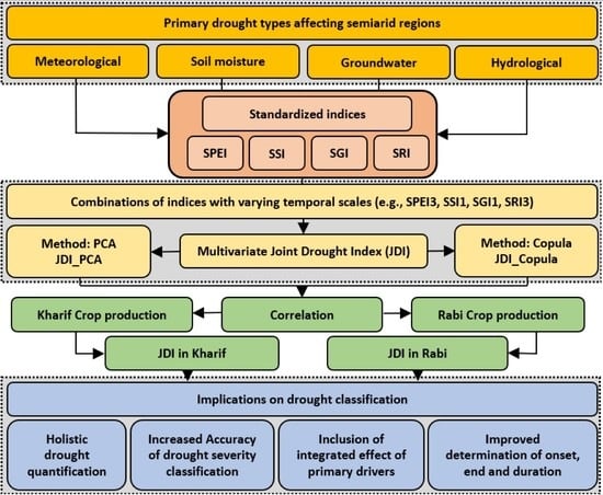
2.2.3. Integration of the Indices in JDI

Multivariate distributions, in general, are mainly focused on statistical properties of drought indices without concern for physical processes that cause a certain time lag [62,84]. In this study, the effect of time lag in response of different variables to climatic conditions [44,85,86] was incorporated by forming JDI with combinations of these variables with different time scale, ranging from 1 to 12 months (1, 2, 3, 4, 6, and 12 months for SPEI, 1 to 3 months for SSI, and 1 to 4 months for SRI and SGI). In total, 288 unique combinations of these indices having different temporal scales were used to generate JDI based on PCA and copula.
Since seasonal crop conditions are directly associated with the prevailing drought conditions, crop yield can presumably be used as an indicator to analyze the accuracy of JDI. Hence, the mean drought intensity of JDI for each season (Kharif and Rabi) was correlated to the standardized crop yield of the respective season to analyze the potential of JDI to capture the drought characteristics. A JDI combination having the highest correlation with the crop yield is assumed to represent the actual drought conditions better than other combinations. We also evaluated the JDI against each integrated index to understand whether the responses of each variable are satisfactorily captured through the integration. The combination giving a highest correlation with the seasonal CP and capturing the optimal response (having the highest correlation with each of its integrated variables) from the integrated variables is then finally selected for the analysis for each season. It is possible that the combination of variables in JDI giving the highest correlation with the seasonal crop yield is different in both seasons. In such a case, different time scale combinations are considered to define JDI and categorize drought in the respective season.
A previous study has verified the consistent use of groundwater for irrigation in semiarid parts of central India, along with its role in vegetation response to hydro-climatological changes [9]. Soil moisture is another important indicator conveying immediate water stress faced by vegetation due to lack of irrigation. Since crop conditions can greatly vary depending on the monthly state of these two variables, a 1-month scale was set for SSI and SGI in deciding the seasonal combination for JDI, along with varying scales of SPEI and SRI. For better representation and easy comparisons, the scales of variables used in the development of JDI are included in the JDI nomenclature, along with the method used. The numbers included the index name representing the temporal scales of SPEI, SSI, SGI, and SRI in the order of appearance. For example, JDI_PCA_3_1_1_3 represents JDI_PCA using SPEI (3 months), SSI (1 month), SGI (1 month), and SRI (3 months). Here, the drought classification scheme by Svoboda et al. [87], based on the percentile approach for magnitude category thresholds, was adopted (Table 1), which is also preferred by many researchers for related studies [33,44,88].

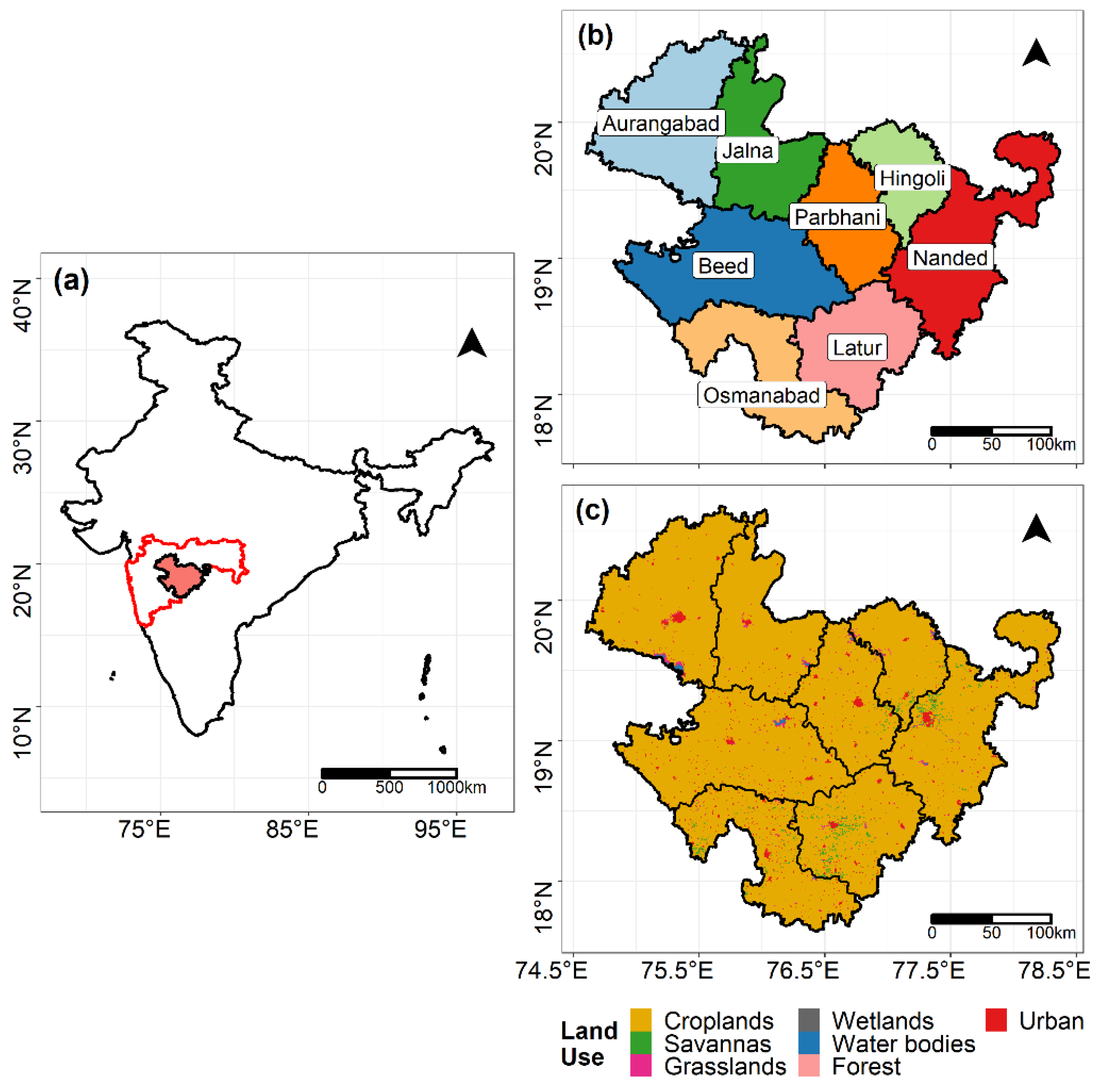
2.3. Case Study Region

In this study, the semiarid region of Aurangabad division, also known as Marathwada, from central state of Maharashtra in India was considered for the development of the JDI (Figure 2). Maharashtra is the largest economy state in India, where more than 50% of the state population depends on agriculture and allied businesses (Figure 2a, Economic Survey Reports of Maharashtra, https://mahades.maharashtra.gov.in/publications.do?pubId=ESM, accessed on 3 November 2021). The region is highly susceptible to drought vulnerabilities and has often seen farmers suicides related to drought and agriculture failures [9,11,89]. Due to Sahyadri mountain ranges running parallel to the west seacoast, the state is mainly divided into two parts: Western Ghats of Kokan to the west and Deccan plateau to the east. A similar distinction is formed in terms of precipitation, which is highly influenced by the Arabian branch of the monsoon coming perpendicular to the Ghats. Marathwada is located in the leeward side of the Sahyadri and consists of eight districts—Aurangabad, Beed, Latur, Osmanabad, Parbhani, Hingoli, Beed, and Nanded (Figure 2b), with an area of about 69,899 km2. The region has a tropical-semiarid climate with four distinct seasons: monsoon (June–September), post-monsoon (October–December), winter (January–February), and summer (March–May). The average annual precipitation of Marathwada is minimum in the state (811 mm), more than 80% of which occurs during four months of monsoon season (Figure S1). There are two main agriculture seasons of the region: Kharif (coincides with monsoon season, i.e., June–September) and Rabi (October–March). The monsoon rainfall is crucial for agriculture, as it is mainly rainfed, where post-monsoon rainfall also plays a key role in the Rabi season and aquifer recharge. Out of four months of monsoon season, Marathwada receives the highest rainfall in July, with August and September having similar intensities (Figure S1). The maximum and minimum monthly temperatures for the region are observed in May (~41 °C) and in December (~13 °C), respectively (Figure S1). Marathwada is underlain by a hard rock aquifer system, where even minor fluctuations in the monsoon rainfall may exaggerate the prevailing drought conditions [90,91], ultimately hampering the various aspects of the agriculture sector. The land is primarily used for agriculture (Figure 2c), where food grains, cereals, pulses, and oilseeds are mainly grown. The arid hydro-climatological conditions are similar over the whole region, which is highly vulnerable to water deficit conditions, further aggravated by lack of adequate infrastructure and developmental backlogs [9,89], where, during 2003–2020, some or the whole of the region was frequently subject to negative precipitation anomalies (which often leads to different types of droughts) (Figure S2).

3. Results

3.1. Selected Combination of Indices for JDI

Amidst all the combinations of SPEI, SSI, SGI, and SRI used to construct JDI, the combination of SPEI (3 months), SSI (1 month), SGI (1 month), and SRI (3 months), represented as 3_1_1_3, was best correlated to CP in Kharif season in both methods, i.e., JDI_PCA and JDI_Copula (Figure 3a,b and Table S1).
Similarly, in Rabi season, a combination of SPEI (6 months), SSI (1 month), SGI (1 month), and SRI (4 months), represented as 6_1_1_4, had the highest correlation with Rabi CP and could be considered to best represent the corresponding drought conditions (Figure 3c,d and Table S1). Furthermore, to evaluate the potential of JDI to incorporate feedback from each integrated variable and to strengthen the choice of the combination, the correlation between the JDIs to each of its four constituent indices was estimated. We found that both JDIs were able to capture the responses from each hydroclimatic variable with strong correlation (Table S2). Although overall correlations of the integrated variables (SPEI, SSI, SGI, and SRI) with JDIs gave comparable responses (Table S2), the correlation of larger scale SRI (3–4 months) with JDI is stronger (r~0.8) than the shorter scale (r~0.5 to 0.7) attributable to the increased accumulation period. Among the hydroclimatic variables used in this study, surface runoff was highly correlated with precipitation (r~0.9), while SM and GWS were highly correlated to precipitation with lagging by 1 month (r~0.8) and 2 months (r~0.8), respectively (Figure S3).

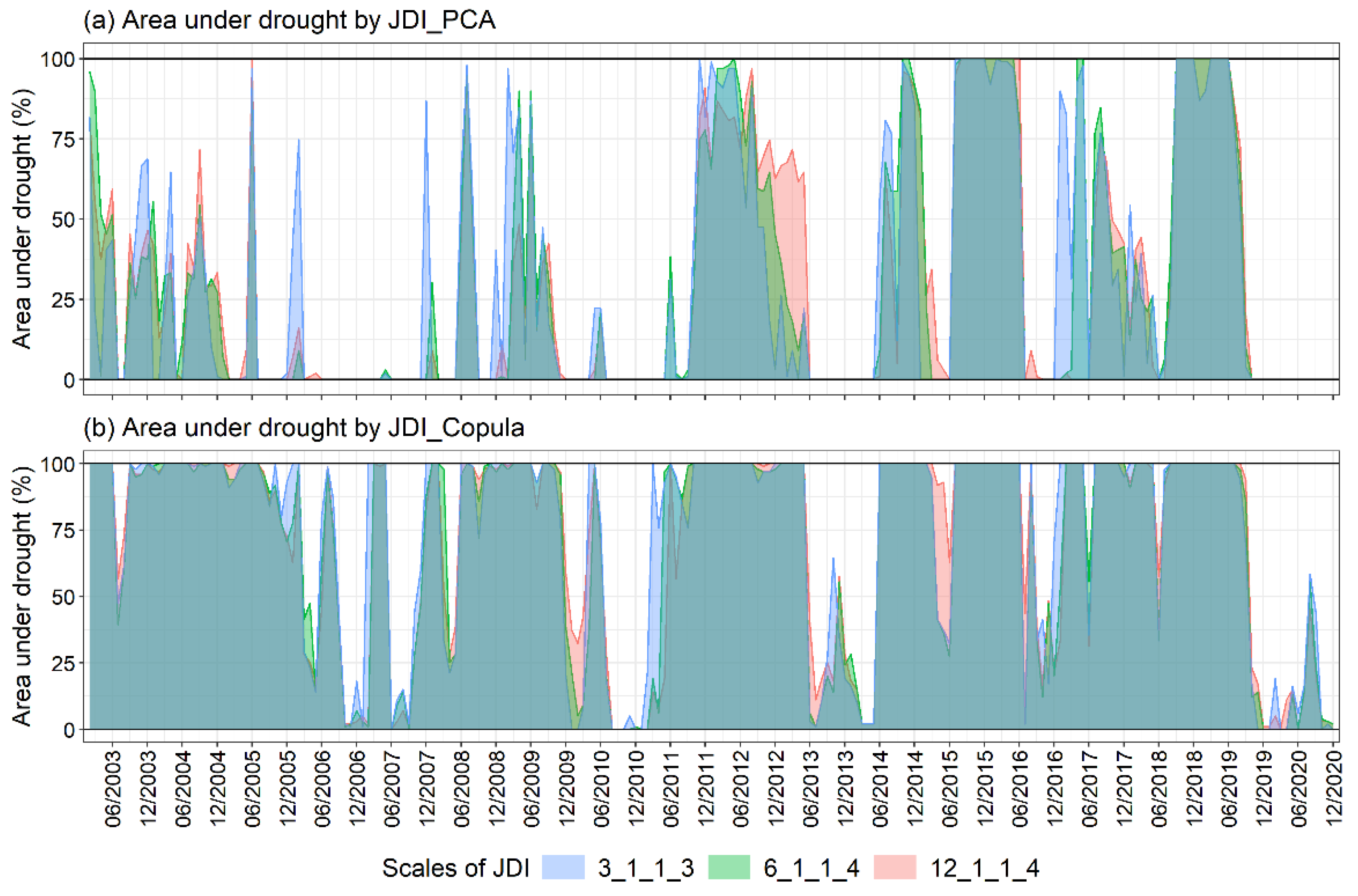
3.2. JDI Based on PCA (JDI_PCA)

The weight of each parameter used for the selected JDI_PCA for average Marathwada in each season and for each month is provided in Table 2. Comparing the contribution of each variable, SPEI and SSI were found to be important variables in both seasons, having higher weights, while the weightage for SGI was higher in Rabi season than Kharif season (Table 2). This can also be seen in the spatial distribution of weight components over the region, associated with the increased use of groundwater in the Rabi season (Figures S4 and S5). We observed that drought intensity estimated by PCA is, in general, an average of the intensities of the integrated variables. In each season, the average weight allocated by PCA to each index is quite comparable (0.26~0.29) (Table 2), except for SGI in Kharif and SRI in Rabi, which have lower weights (average of the season, 0.18 and 0.19, respectively) than other variables in respective seasons.
Apart from monthly weights, JDI_PCA using seasonal weights (four weights per season, total eight for Kharif and Rabi) was also evaluated using the same process as discussed in Section 2.2.1, where a similar phenomenon was observed when SGI was given higher weight in Rabi than in Kharif season (Table S3). It should be noted that the intensities by JDI_PCA using monthly and seasonal weights were very highly correlated (r > 0.95; Figure S6), subject to the similarity in weights for the integrated indices. Despite this similarity, to even capture any slight changes in the JDI response to monthly variations in the hydro-climatic variables, monthly weights were used in this analysis.

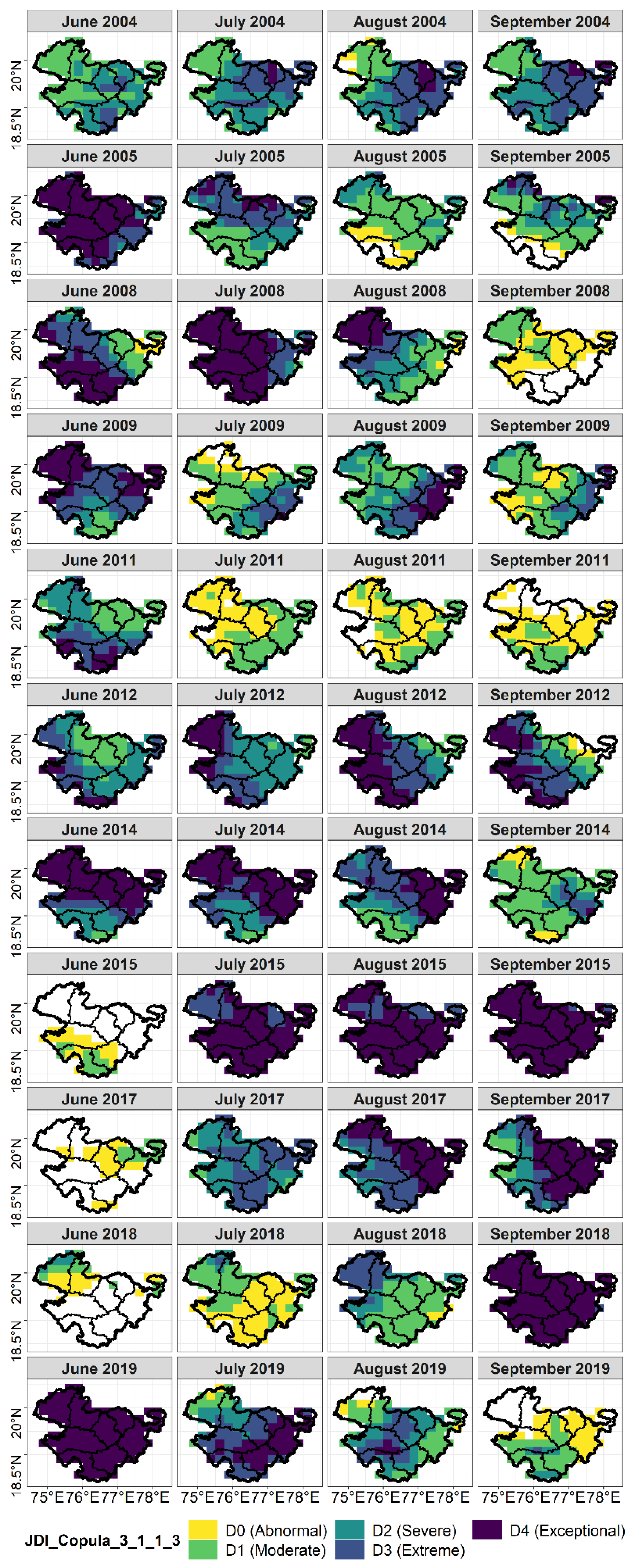
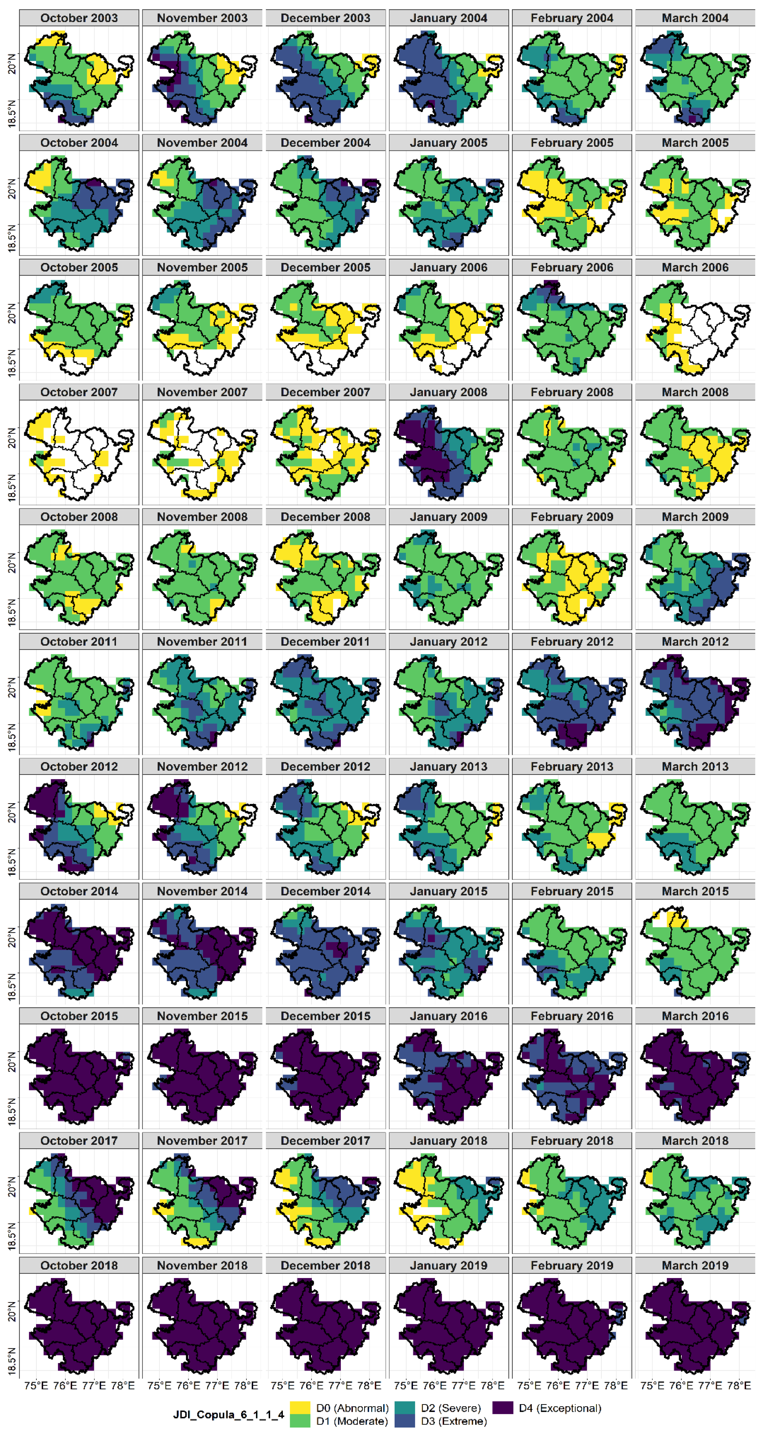
3.3. JDI Based on Copula (JDI_Copula)

The classical AIC and BIC criteria show that, among the selected family of copulas, Gaussian copula can best represent the joint distribution of hydroclimatic variables (Table 3). The JDI_Copula using Gaussian transformation for Kharif and Rabi season also satisfy the Sn and Tn statistics, with a p-value greater than 0.05. Spatially, 99% of grid points over the region satisfy the Sn and Tn criteria in Kharif season, while, in Rabi season, the percentage is 97% and 90%, respectively (Figure S7). Moreover, as the scale of SPEI in JDI increases, the number of grid points satisfying the goodness-of-fit criterion decreases (85% and 81% of grid points satisfy Sn and Tn criterion, respectively, for JDI_Copula_12_1_1_4).
Figure 4 shows the time series of both the JDIs in the Kharif and Rabi seasons, along with the variables used for the integration. It was observed that JDI_PCA and JDI_Copula are highly correlated with each other (r > 0.95) in both seasons (Figure S8). If there is a drought in any one of the integrated variables, there is a higher chance of its detection by copula than PCA, as copula constitutes a larger probability space [63,74]. Notwithstanding the normal conditions in other variables, if there is drought in a single integrated variable, JDI_Copula will indicate a drought situation (for example, in year 2005 in Figure 4a,b), due to severe conditions in SGI, JDI_Copula displayed more severe intensities than JDI_PCA). More severe behavior is displayed when all the variables are excessively diverted towards the negative side, where JDI_Copula will show exceptional drought conditions compared to the integrated variables (for example, the years 2015 and 2018 in Figure 4a,b)). JDI_PCA, on the other hand, tries to optimize the responses from the individual variables through linear transformation by taking maximum information from each integrated variable in the form of a principal component and, consequently, the weight component (Figure 4).

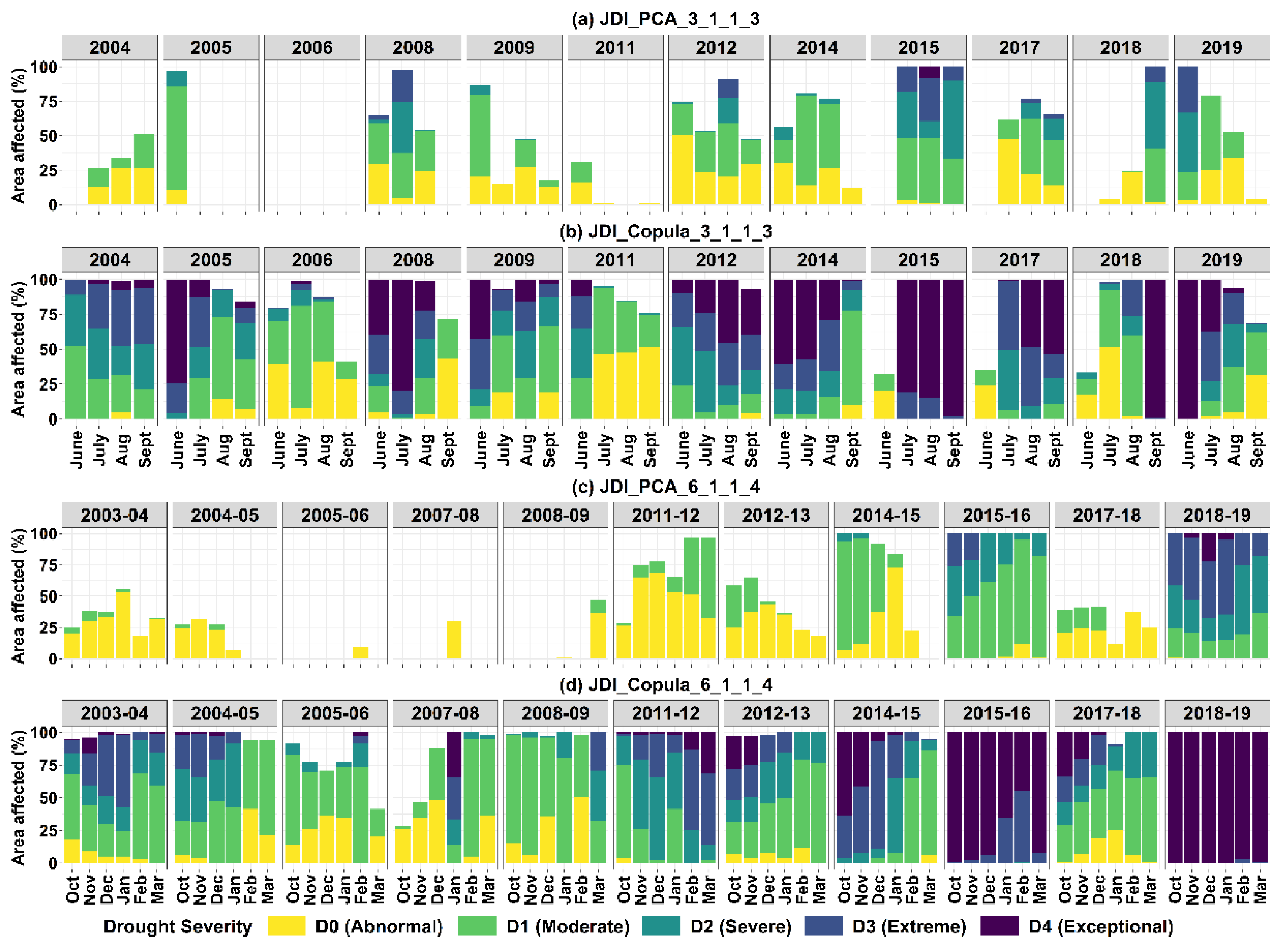
3.4. Seasonal Analysis of the Drought Intensities

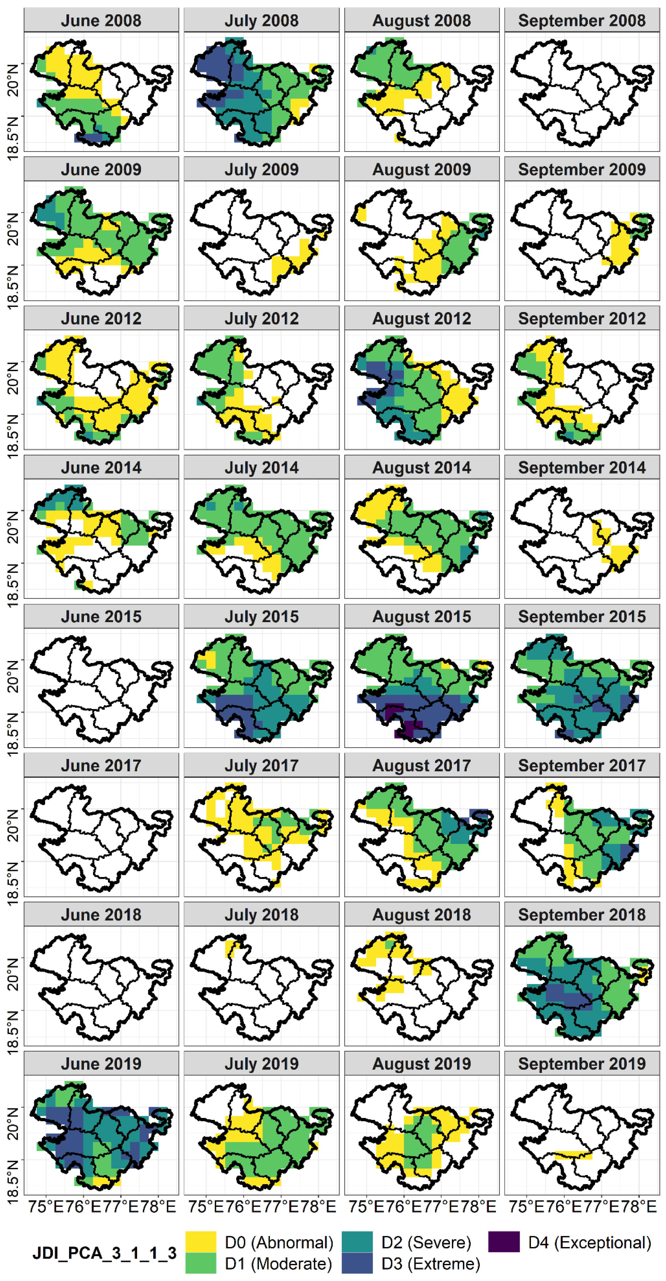
3.4.1. Kharif Season
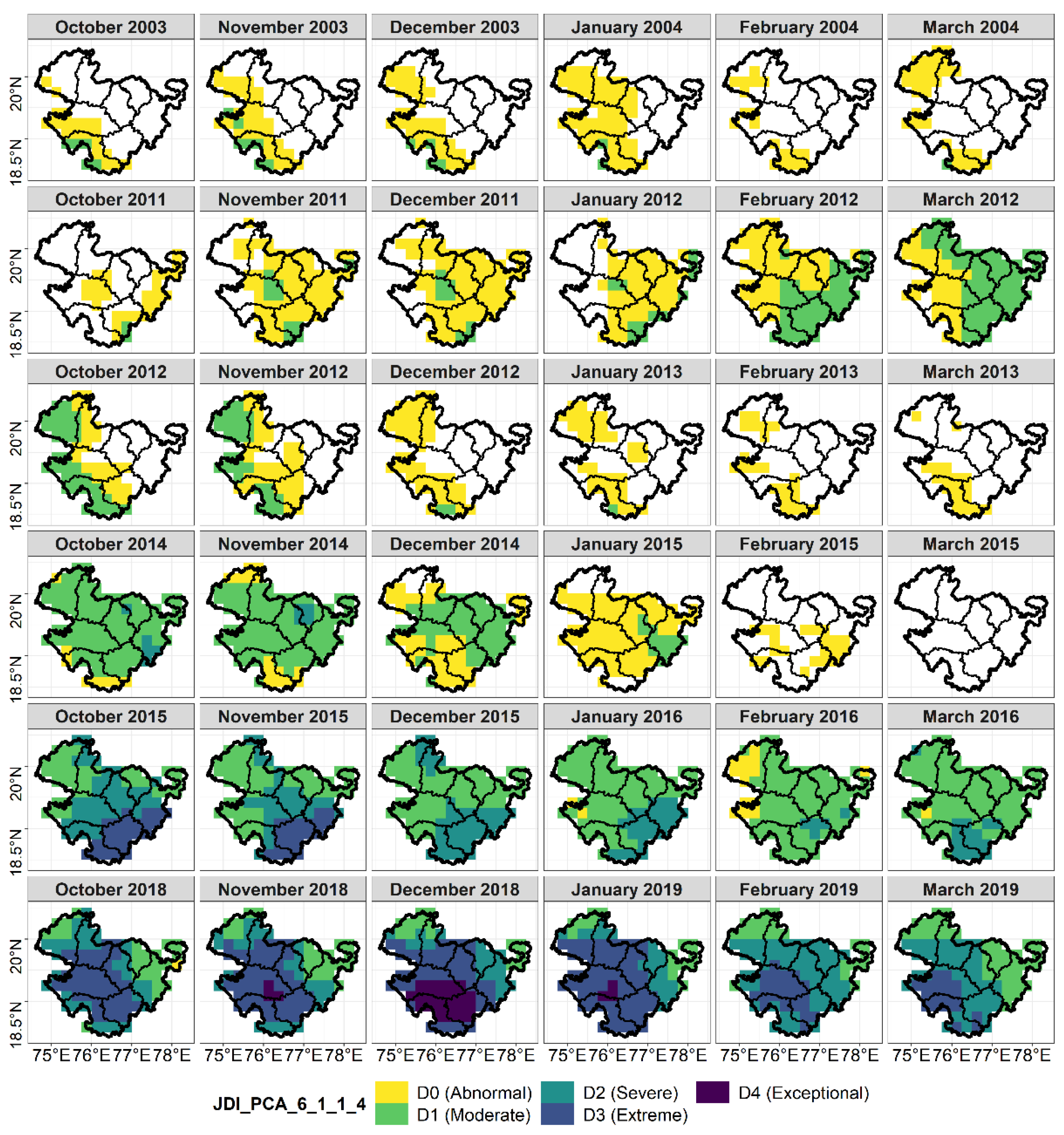
During four months of the Kharif season, JDI_PCA detected a minimum of three, while JDI_Copula detected a minimum of nine drought events in June and September, respectively. One interesting finding is that, despite receiving ample monsoon rainfall (173 mm, Figure S1), the month of August witnessed the highest drought frequency (number of drought events) in both methods (Figure S9a). We found that the detection of drought events using JDI_Copula was much higher than that of JDI_PCA pertaining to more severe drought intensities. Spatially, Marathwada showed a minimum of seven droughts in each month per pixel detected by JDI_Copula, which is just two in the case of JDI_PCA (except for few pixels showing only one drought in January and February (Figure S10a,b)).
The drought conditions in any month of the Kharif season are crucial for farmers, as they affect overall crop performance for the season. The analysis of the spatial distribution of various drought events detected by JDI_PCA revealed that, in year 2015, 100% of the Marathwada region was under moderate to extreme drought, except for June (Figure 5 and Figure 6a). The onset of the monsoon in the year 2015 was normal, with no drought conditions in June (Figure 5). However, the remaining months of the season experienced severe to extreme drought conditions, especially in the southern part of the region, causing overall Kharif crop losses of more than 60% (Figure S11), where parts of Osmanabad district also recorded exceptional drought conditions in August. Similar characteristics of the 2015 drought were also registered by JDI_Copula, with some differences in the drought intensities (JDI_Copula showed exceptional drought conditions over the entire region, Figure 6b and Figure 7). In both methods, a linear decreasing trend in drought severity was observed in the Kharif season (except for June), which suggests an increase in drought intensities and frequency (Figure S9a). However, the trend was not significant.
In most of the drought years recorded by JDI_Copula, 100% of the region showed drought conditions ranging from moderate to exceptional categories, with certain pockets having at least abnormally dry conditions (Figure 6b and Figure 7). JDI_Copula exhibited a tendency to show exceptional drought conditions in cases of severe droughts in JDI_PCA by encapsulating every response of the integrated variables. This resulted in higher drought intensities by JDI_Copula, such as in the last three months of the Kharif season of 2015, where 100% of the area was shown to be under exceptional drought conditions (Figure 6b and Figure 7). The difference in the intensities of the drought severity by both methods is especially evident in the initial years of the analysis (Figure 6). For example, in 2005, JDI_PCA showed moderate drought conditions in June, while the conditions were exceptional by JDI_Copula during the same period, while, in other months, only JDI_Copula showed drought conditions with varying intensities over the region, with no drought detection by JDI_PCA (Figure 6a,b). Detailed analysis of the integrated variables for the Kharif season of 2005 showed that the entire region of Marathwada was under meteorological drought in June, while only Aurangabad district in the northwest suffered from extreme to moderate drought conditions in three months of the season (Figure S12 for SPEI 3, 2005). In the same year, groundwater displayed severe drought conditions covering the entire area during the same period, whereas SSI and SRI exhibited normal conditions, except for June (Figure S12 for SSI 2005, SGI 2005, and SRI 2005). As PCA allocates lower weights to SGI in Kharif season and pertaining to comparatively higher contribution from other integrated variables (Table 2), JDI_PCA averages the responses, and the drought severity was not significant by JDI_PCA in 2005, except for June. Consequently, by capturing this groundwater drought, JDI_Copula exhibited exceptional to moderate drought conditions throughout the season of 2005. In conclusion, JDI_Copula was more efficient in capturing the groundwater drought than JDI_PCA.

3.4.2. Rabi Season

Rabi season in Marathwada primarily depends on the groundwater for irrigation and lasts for about six months, from October to March. We observed similar characteristics of JDI_PCA and JDI_Copula in the Rabi season as those in Kharif, where JDI_Copula was able to record a higher number of drought events than JDI_PCA (Figure 6c,d and Figure S9b). The number of drought occurrences is lower in December (JDI_Copula) and January (JDI_PCA) compared to other months, which, again, increased in February and March as the season progressed (Figure S9b).
In the Rabi season, JDI_PCA showed abnormal to moderate drought conditions in most of its captured events (Figure 8). During these events, 100% areal coverage over the study area was observed for only two drought years, i.e., 2015–2016 and 2018–2019, with more severe intensities than the rest of the events (Figure 6c and Figure 8; 2015–2016 represents Rabi season from October 2015 to March 2016. Same for other years). JDI_Copula, on the other hand, showed 100% of the area under drought during most of the events by capturing the integrated response of the involved hydroclimatic variables and water storage deficits, with higher drought intensities than JDI_PCA (Figure 6d and Figure 9). Rabi seasons of 2015–2016 and 2018–2019 were particularly critical for Marathwada. Pertaining to higher (negative) precipitation anomalies in the Kharif season of 2015, the Rabi season of 2015–2016 experienced severe to exceptional drought conditions throughout (Figure 8 and Figure 9), bringing down the Rabi CP to about 65% of the average (Figure S11). Likewise, in 2018–2019, the drought conditions were extreme to exceptional during the whole season, covering the entire area and causing a loss of around 42% in the Rabi CP (Figure 8, Figure 9, and Figure S11). During both years, the preceding Kharif season had suffered from severe to exceptional drought conditions. However, in 2018–2019, with respect to drought in the earlier Kharif season, the crop area was already lowered by about 35% (https://mahades.maharashtra.gov.in/, accessed on 3 November 2021). This may be one of the reasons behind comparatively less loss of Rabi production in 2018–2019, despite having severe drought conditions compared to 2015–2016.

3.5. Multiseason and Multiyear Droughts

Multiseason droughts gravely impact the ability of the farmers to deal with drought situations by seizing their financial capabilities due to agriculture losses in the current season in conjunction with the previous one. During 18 years of analysis, Marathwada was subject to several drought events spanning multiple seasons and sometimes extending up to years (Figure 10). We considered the season to be drought-affected when the drought conditions were observed for three consecutive months in both the seasons and in any of the three months for the Kharif season. If the drought situation possesses sporadic breaks of one or two months owing to the anonymously heavy localized precipitation, those months were also included in the drought duration. For April and May, scale 6_1_1_4, in continuation to Rabi season, was considered to analyze the drought intensity.
Considering the difference in the recorded intensities by both the methods, multiyear droughts recorded by JDI_Copula persisted longer and were more severe than those by JDI_PCA. For example, a 13-month drought was recorded by JDI_PCA, which started from November of the Rabi season of 2011–2012 and continued to the Kharif season in 2012, with a slight extension in the following Rabi season (Figure 10). The same drought was recorded by JDI_Copula, starting from Kharif in 2011 and ending in Rabi 2012–2013, with a duration of about 24 months (Figure 10). Similarly, with a gap of a few months in Rabi season of 2014–2015, the drought starting in 2014 also continued till the Rabi season of 2015–2016, making 2015 the most critical drought year in Marathwada (Figure 10, [92]). Although there is no specific crop season in the summer months of April and May, severe drought conditions in these months increase the land surface temperature and soil moisture demands of the following Kharif season. Similar behavior can be observed in the persistent drought conditions in 2017, which started in February 2017 and continued till the end of the Kharif season. Although there are no particularly abnormal drought conditions shown by JDI_PCA for the remaining season of 2017–2018, the conditions were below normal, causing soil moisture deficit and stress in the crops, which caused a decrease in the Rabi CP compared to the previous year (Figure S11). In contrast, JDI_Copula discerned the multiyear drought conditions from February 2017 until August 2019, covering drought conditions of years 2017–2018, as well as the severity of drought in 2018–2019 (Figure 10). JDI_Copula also unveiled the incessant multiyear drought conditions starting from February 2003 to August 2006, together with some recoveries in Kharif of 2003 and in end of the Rabi season of 2005–2006, which were typically absent in JDI_PCA (Figure 10). Although below normal (JDI = 0) conditions can be observed for JDI_PCA for a majority of this period, the drought severity detected by JDI_PCA was negligible. Detailed analysis for each integrated index for this period suggests abnormal groundwater conditions over this region, which was satisfactorily captured by JDI_Copula (Figures S12 and S13). These results compare well with the recorded CP anomalies. The Rabi CP in 2003–2004 and 2004–2005 was lower by 40% and 20%, respectively, while, for 2005–2006, it was slightly higher by 5% (Figure S11). Despite abnormal groundwater conditions in Kharif in 2005, other variables contributed to improving the CP by approximately 11%, which, again, decreased in 2006, mostly due to the persistent groundwater anomalies and drought conditions in the initial months of the season (Figures S11 and S12). Although category D0 leans towards the recovery of the drought, prolonged exposure to abnormal conditions causes many lingering hazards (environmental, social, etc.). We observed that JDI_Copula was highly effective in analyzing the drought conditions covering multiple drought parameters compared to JDI_PCA and can, therefore, be used to predict the CP anomalies in the respective season.

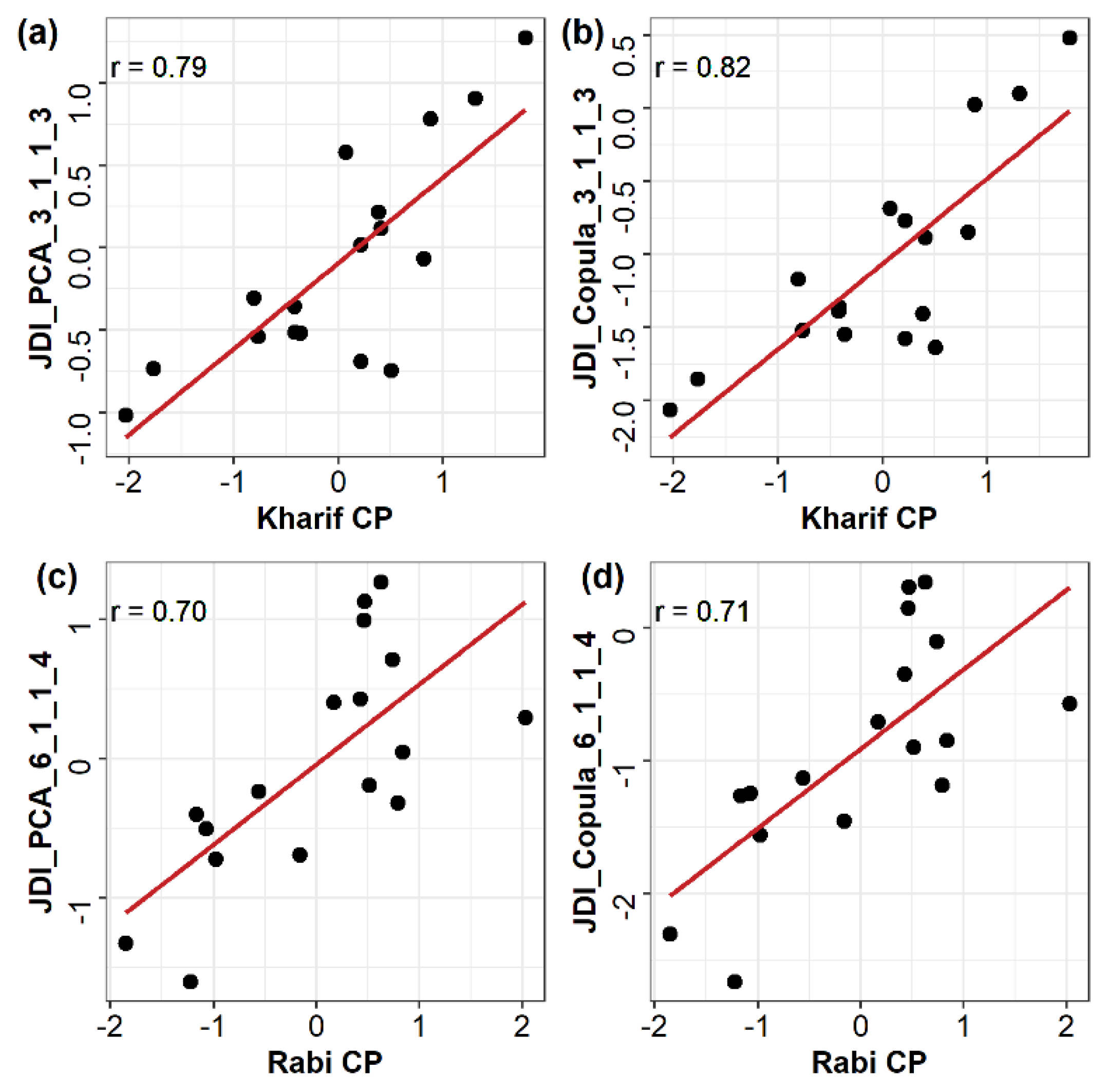
3.6. Prediction of CP from JDI

The significant association between CP and JDI can be established for copulas through a regression equation, where the p-values for both the intercept and the slope were significant (p < 0.05; while, for PCA, p > 0.05 for the intercept). Thus, JDI_Copula_3_1_1_3 was used to predict the CP in the Kharif season with Equation (4) and JDI_Copula_6_1_1_4 for Rabi CP prediction using Equation (5).
Kharif CP = 1.21 + 1.14 × JDI_Copula_3_1_1_3 (r = 0.82)
Rabi CP = 0.76 + 0.84 × JDI_Copula_6_1_1_4 (r = 0.71)
The CP is particularly sensitive for JDI values in Kharif season associated with the volatile monsoon precipitation characteristics and its influence on the indices integrated in the JDI (deviation of ±0.1 in JDI shows fluctuation of ~22.8% and ~16.8% in Kharif and Rabi CP, respectively).

4. Discussion

The multivariate drought indices JDI_PCA and JDI_Copula prove to be potentially competent and coherent in capturing the responses of each integrated hydroclimatic variable and overall water deficit conditions of the study region in the case of drought. Although different combinations of SPEI (3 and 6 months), SSI (1 month), SGI (1 month), and SRI (3 and 4 months) were used for the development of JDI, there is no fixed effective and common (applicable everywhere) combination of indices to construct the joint index. Closely related combinations were found to exhibit comparable correlations with the crop yield and showed similar drought intensities (Table S1 and Figure S14a–d). However, when the time scale of the integrated index is longer, it often involves conditions that no longer influence the current hydrological situations, which can result in higher correlation between the JDI and the CP [72,87] (for example, scale 12_1_1_4 in Table S1). JDI with different combinations of integrated indices are found to be highly correlated with each other (Tables S4 and S5). The difference in these JDIs lies in the persistence of the drought with change in the scale of any variable in the combination as the drought progresses (Figure S14e,f). When there is a difference in the accumulation period (scale) of any one index of the combination, the response of JDI differs accordingly. Shorter scale indices attain positive values more quickly, while longer scale indices persist over a longer period (Figure S14e,f). For example, JDI_PCA, as well as JDI_Copula for the shorter scale (3_1_1_3), show higher drought intensity for June 2014, while longer scale indices (6_1_1_4 and 12_1_1_4) remain at comparatively lower intensities (Figure S14e,f) for June 2014. Moreover, partial drought recoveries are captured more effectively by JDI having lower scale SPEI by reducing the drought intensities, while JDI with 12-month SPEI still shows severe drought conditions (e.g., from December 2015 to June 2016, Figure S14e,f). Drought intensities in Kharif season are more efficiently captured by scale 3_1_1_3 by both JDIs than scale 6_1_1_4 (e.g., Kharif 2014 and 2015 in Figure S14e,f), while, for Rabi season, scale 3_1_1_3 shows higher intensities than scale 6_1_1_4 (e.g., Rabi season 2005–2006, 2010–2011, and 2016–2017, Figure S14e,f). While JDI intensities for Kharif season are more comparable for both the scales (3_1_1_3 and 6_1_1_4) used in this analysis (Figure S15a,b), there is higher variability of drought intensities in Rabi season (Figure S15c,d). This shows that separate indices, using appropriate scale variables for integration, used to define the seasonal drought characteristics provide more realistic results than using a single index for analyzing the drought for the whole year. An area under drought by differently scaled JDIs also shows variations with higher persistence of JDIs involving longer scale indices (Figure 11). Moreover, the area under drought by JDI_PCA varies considerably with JDI_Copula, where 100% of the area is frequently under drought (Figure 11).
The probability of agricultural drought occurrence increases with increase in the severity of meteorological drought [93]. Integrated indices, such as JDI, play an important role in capturing the drought conditions created by different hydro-climatological abnormalities. The periodic precipitation spells may improve the meteorological drought conditions temporarily depending on the precipitation volume, subsequent meteorological conditions, crop growing stage, and cropping seasons and patterns. However, it may not ameliorate the agricultural, groundwater, or hydrological drought conditions, as observed for the initial years of the analysis. JDI reasonably incorporates responses of all the integrated variables and, thus, puts forward an improved understanding of the drought onset, which is crucial for employing the mitigation strategies by the governing agencies. In particular, JDI_Copula is more efficient in capturing the groundwater drought than JDI_PCA, as observed in this analysis. However, as copula tries to consider the critical responses from each integrated variable, JDI_Copula might give lower estimates, even in wet periods, similar to the higher estimates in the case of droughts.
PCA and copula both possess the potential to be included in the drought management of India, avoiding separate judgment of individual indices, which may not always capture the integrated effect. Groundwater, being the main source of irrigation, has major influence on the drought conditions in the region as observed by JDI_Copula. JDI_PCA’s limitation lies in the fact that it is essentially a linear combination of the drought indices assumed to represent maximum information from each variable through the variance [62]. JDI_Copula, on the other hand, preserves the marginal distributions of the integrated variables and their dependence structure. Although both JDIs are highly correlated and have a similar direction of the drought intensities, the captured drought intensity varies considerably, with JDI_Copula frequently showing exceptional drought conditions. Similar observations were reported by other studies, indicating the ability of copula-based integrated index to capture extreme drought conditions better than other methods (e.g., entropy) [94]. However, this may not be advisable for the mitigation measures, as this overestimation may stress the official resources to always deal with extreme conditions. Nevertheless, the standardized JDI_Copula and standardized JDI_PCA (removing the mean and dividing by standard deviation) give more similar drought intensities, where extreme behaviors are better captured by JDI_Copula (Figure S16). Determination of the threshold for the drought categorization is, however, a subjective assumption, where upscaling or downscaling the threshold may result in changes in the drought severities and area under drought. Despite these, JDI_Copula is recommended for evaluating the overall drought conditions with due consideration to the response from every critical variable in the region, whereas JDI_PCA can be used to inspect the average integrated response of regional drought characteristics. Considering the wide impacts of droughts and their involved complexity, qualitative depictions of drought impacts are as necessary as quantitative analysis. Synergizing the regional expert knowledge from local bodies, agriculturists, and climatologists is also critical for drought categorization and can play an important role in the interpretation of JDI to correctly capture the drought impacts. Furthermore, such multidisciplinary considerations will also play a critical role in identifying weak links in the drought monitoring system and for future mitigation strategies [95], especially in vulnerable regions, such as Marathwada.

5. Limitations and Future Scope

Although multivariate drought indices, such as JDI, enhance the collective detection of various types of droughts, they may not overpower the ability of the univariate indices to apprehend the drought characteristics, nor are they inherently superior. When a single drought type, such as meteorological, is to be analyzed, a single standardized index, such as SPI/SPEI, can still give better insights. Moreover, independent hydrological model simulations at regional scales may provide more sophisticated inputs for integrated indices than readily available LSM outputs, which needs further research. Here, we recognize that longer time-series data would be more beneficial for standardized indices of GLDAS model outputs, which also reflect the associated uncertainties. Nevertheless, JDI displays the potential to be used for the assessment of local hydro-climatological conditions, leading to improved current and future drought assessment techniques. Fine-resolution vegetation indices, such as NDVI and VCI, can also be used along with JDI for enhanced spatial details of drought conditions. The lack of high-resolution and seasonal CP data hinders the accuracy in the assessment of drought severity. However, the approach of using a separate multivariate index for each season, representing the seasonal crop conditions by the highest correlation, as discussed in this study, will be beneficial in drought mitigation over any region by increasing the accuracy of drought detection. Weekly monitoring, particularly in Kharif season, may be beneficial in the timely detection of drought aggression and effective mitigation measures. Socioeconomic drought, although difficult to include in multivariate index, should be contemplated in future drought analysis, considering its grave impacts. More evolutions are anticipated in JDI by incorporating the locally/regionally critical drought indicators.

6. Conclusions

In this study, a multivariate joint drought index (JDI) was developed by integrating standardized indices representing meteorological (SPEI), soil moisture (SSI), groundwater (SGI), and surface runoff (SRI) drought by using PCA and Gaussian copula. Various combinations of these indices were analyzed for correlation with seasonal crop production (CP), and the combination showing the highest correlation was selected for the assessment of drought conditions in the Marathwada region of central India. The key findings of this study are as follows:
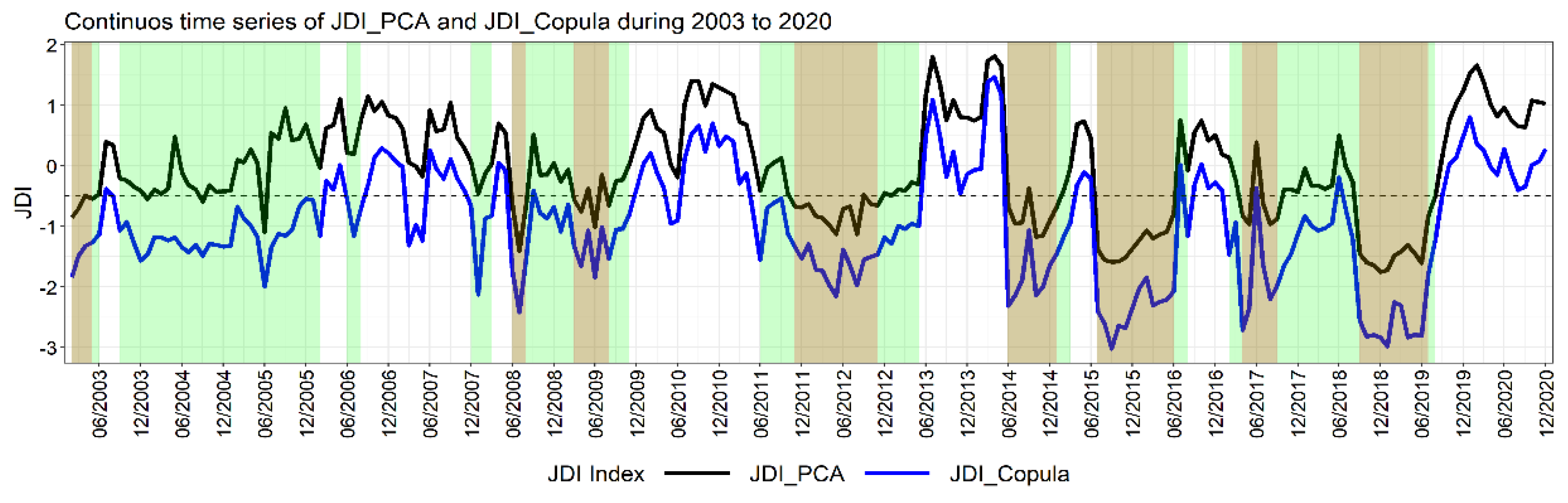
  • Unlike traditional indices, JDI efficiently captured the combined effect of drought variability in the study region. Moreover, the dynamics of seasonal CP and JDI corroborate each other, showing the advantages of using separate JDI for drought analysis in each season. JDI_Copula performed better in detecting the extreme drought characteristics by each integrated variable by preserving their dependence structure than JDI_PCA, which averaged the responses.
  • Groundwater, being the primary source of irrigation, is an important driver of droughts over Marathwada, shaping the regional drought characteristics. JDI successfully captured this contribution, revealing its potential to support local-scale decision making and the ability to be evolved for any region having different hydroclimatic conditions by integrating locally critical inputs (e.g., snow accumulation, reservoir storage, fire risks, etc.).
  • Multivariate indices are more efficient in capturing overall water deficit from multiple drought-related indices compared to a univariate index. JDI, as presented in this study, can play a crucial role in drought analysis with improved accuracy of detection of each drought type and comprehensive inclusion of various seasonal drought characteristics.
  • JDI proves to be efficient in detecting the onset, termination, and duration of drought based on the integrated effect of multiple drought indicators, which otherwise was difficult to analyze. Out of drought characteristics captured by both the methods, droughts of the years 2015–2016 and 2018–2019 were the most severe in the study region.
  • The results of this study also highlight the importance of a multidisciplinary approach in drought classification, which can play a crucial role in policy formation and food security, by providing a timely and accurate estimation of drought characteristics by reducing the inherent inconsistencies in the traditional methods. This is also important for the socioeconomic security of vulnerable regions, such as Marathwada, experiencing increased suffering of the farmers.
The novel approach of seasonal drought categorization for holistic quantification of drought conditions, as presented in this study, should provide a unique perspective to drought monitoring by increasing the accuracy of drought severity analysis worldwide.

Supplementary Materials

The following supporting information can be downloaded at: https://www.mdpi.com/article/10.3390/rs14163891/s1, Figure S1: Long-term (1989–2020) mean monthly precipitation and minimum and maximum temperature in Marathwada; Figure S2: Monsoon precipitation anomaly over Marathwada from 2003 to 2020; Figure S3: Mean monthly precipitation, surface runoff, soil moisture, and groundwater storage over Marathwada region from 2003 to 2020; Figure S4: Weight allocation to each hydroclimatic variable in each month by PCA in Kharif season (JDI_PCA_3_1_1_3); Figure S5: Weight allocation to each hydroclimatic variable in each month by PCA in Rabi season (JDI_PCA_6_1_1_4); Figure S6: Scatterplot of JDI_PCA intensities using monthly weights and seasonal weights obtained by process discussed in Section 2.2.1 on monthly data and seasonal data of each year during 2003–2020; Figure S7: Significance value (p value) for Cramer–von Mises statistic (Sn) and Kolmogorov–Smirnov statistic (Tn) for Gaussian copula in Kharif season (a,b; JDI_Copula_3_1_1_3) and Rabi season (c,d; JDI_Copula_6_1_1_4); Figure S8: Scatterplot showing correlation between JDI_PCA and JDI_Copula for Kharif (scale 3_1_1_3) and Rabi (scale 6_1_1_4) season for average Marathwada (a,b, r~0.95) and spatial correlation of the same in each season (c,d); Figure S9: Time series of JDI_PCA and JDI_Copula in each month of (a) Kharif (June to September) and (b) Rabi (October to March) season during 2003 to 2020; Figure S10: Number of moderate to exceptional drought events in each month of Kharif and Rabi season during 2003 to 2020 using (a) JDI_PCA and (b) JDI_Copula; Figure S11: Crop production (CP) anomaly in Kharif and Rabi season during 2003–2019; Figure S12: Spatial drought severity over Marathwada in Kharif season in each index, i.e., SPEI (3 months), SSI (1 month), SGI (1 month), and SRI (3 months) for the year 2004, 2005, and 2006; Figure S13: Spatial drought severity in Rabi season in each index, i.e., SPEI (6 months), SSI (1 month), SGI (1 month), and SRI (4 months) for the year 2003–2004, 2004–2005, and 2005–2006; Figure S14: Time series of JDI_PCA and JDI_Copula with different combinations; Figure S15: Scatterplot of JDI_PCA and JDI_Copula for scales 3_1_1_3 and 6_1_1_4 analyzed for Kharif months (a,b) and Rabi months (c and d); Figure S16: Scatterplot of standardized JDI_PCA and standardized JDI_Copula obtained by removing the mean and dividing by standard deviation; Table S1: Correlation of mean drought intensities by JDI_PCA and JDI_Copula with standardized crop productions in Kharif and Rabi seasons for different combinations of the integrated indices; Table S2: Correlation of JDI_PCA and JDI_Copula with their integrated indices for different combinations; Table S3: Seasonal weights of indices for JDI_PCA in Kharif (scale 3_1_1_3) and Rabi (scale 6_1_1_4) season; Table S4: Correlation between JDI_PCAs having different combinations of the integrated indices; Table S5: Correlation between JDI_Copulas having different combinations of the integrated indices.

Author Contributions

Conceptualization, K.B.; methodology, K.B.; software, K.B.; validation, K.B., A. and T.K.; formal analysis, K.B.; investigation, K.B.; resources, K.B.; data curation, K.B.; writing—original draft preparation, K.B.; writing—review and editing, K.B., A. and T.K.; visualization, K.B.; supervision, T.K. All authors have read and agreed to the published version of the manuscript.

Funding

This research received no external funding.

Data Availability Statement

All the datasets used in this study are open access.

Acknowledgments

We acknowledge the open-access data provided by various agencies, as referenced in the main text.

Conflicts of Interest

The authors declare no conflict of interest.

References

  1. UNCCD. Drought in Numbers 2022—Restoration for Readiness and Resilience. Available online: https://www.unccd.int/sites/default/files/2022-05/DroughtinNumbers.pdf (accessed on 27 May 2022).
  2. Wilhite, D.A. (Ed.) Drought as a Natural Hazard. In Droughts, 1st ed.; Routledge: Oxfordshire, UK, 2000; pp. 3–18. [Google Scholar] [CrossRef]
  3. Guha-Sapir, D.; Below, R.; Hoyois, P. EM-DAT: The CRED/OFDA International Disaster Database. Available online: www.emdat.be (accessed on 27 May 2022).
  4. Mishra, A.K.; Singh, V.P. A Review of Drought Concepts. J. Hydrol. 2010, 391, 202–216. [Google Scholar] [CrossRef]
  5. Dai, A. Increasing Drought under Global Warming in Observations and Models. Nat. Clim. Chang. 2013, 3, 52–58. [Google Scholar] [CrossRef]
  6. Aadhar, S.; Mishra, V. Impact of Climate Change on Drought Frequency over India. In Climate Change and Water Resources in India; Ministry of Environment, Forest and Climate Change: New Delhi, India, 2018; pp. 117–129. [Google Scholar]
  7. Bloomfield, J.P.; Marchant, B.P.; McKenzie, A.A. Changes in Groundwater Drought Associated with Anthropogenic Warming. Hydrol. Earth Syst. Sci. 2019, 23, 1393–1408. [Google Scholar] [CrossRef]
  8. Government of India. Manual for Drought Management; Ministry of Agriculture and Farmers Welfare: New Delhi, India, 2016. [Google Scholar]
  9. Bageshree, K.; Abhishek; Kinouchi, T. Unraveling the Multiple Drivers of Greening-Browning and Leaf Area Variability in a Socioeconomically Sensitive. Climate 2022, 10, 70. [Google Scholar] [CrossRef]
  10. Talule, D. Farmer Suicides in Maharashtra, 2001-2018 Trends across Marathwada and Vidarbha. Econ. Polit. Wkly. 2020, 55, 1538–1545. [Google Scholar]
  11. Talule, D. Suicide by Maharashtra Farmers, The Signs of Persistent Agrarian Distress. Econ. Polit. Wkly. 2021, 56, 10. [Google Scholar]
  12. Merriott, D. Factors Associated with the Farmer Suicide Crisis in India. J. Epidemiol. Glob. Health 2016, 6, 217–227. [Google Scholar] [CrossRef]
  13. Nagaraj, K.; Sainath, P.; Rukmani, R.; Gopinath, R. Farmers’ Suicides in India: Magnitudes, Trends, and Spatial Patterns, 1997–2012. Rev. Agrar. Stud. 2014, 4, 1997–2012. [Google Scholar]
  14. Iyer, K. Landscapes of Loss: The Story of an Indian Drought; HarperCollins Publishers: Nodia, India, 2021; ISBN 9390327466. [Google Scholar]
  15. Mishra, V.; Tiwari, A.D.; Aadhar, S.; Shah, R.; Xiao, M.; Pai, D.S.; Lettenmaier, D. Drought and Famine in India, 1870–2016. Geophys. Res. Lett. 2019, 46, 2075–2083. [Google Scholar] [CrossRef]
  16. Rodell, M.; Velicogna, I.; Famiglietti, J.S. Satellite-Based Estimates of Groundwater Depletion in India. Nature 2009, 460, 999–1002. [Google Scholar] [CrossRef]
  17. Asoka, A.; Mishra, V. A Strong Linkage between Seasonal Crop Growth and Groundwater Storage Variability in India. J. Hydrometeorol. 2020, 22, 125–138. [Google Scholar] [CrossRef]
  18. Aghakouchak, A.; Farahmand, A.; Melton, F.S.; Teixeira, J.; Anderson, M.C.; Wardlow, B.D.; Hain, C.R. Reviews of Geophysics Remote Sensing of Drought: Progress, Challenges. Rev. Geophys. 2015, 53, 1–29. [Google Scholar] [CrossRef]
  19. Palmer, W.C. Keeping Track of Crop Moisture Conditions, Nationwide: The New Crop Moisture Index. Weatherwise 2010, 21, 156–161. [Google Scholar] [CrossRef]
  20. Mckee, T.B.; Doesken, N.J.; Kleist, J. The relationship of drought frequency and duration to time scales. In Proceedings of the Eighth Conference on Applied Climatology, Anaheim, CA, USA, 17–22 January 1993; pp. 17–22. [Google Scholar]
  21. Vicente-Serrano, S.M.; Beguería, S.; López-Moreno, J.I. A Multiscalar Drought Index Sensitive to Global Warming: The Standardized Precipitation Evapotranspiration Index. J. Clim. 2010, 23, 1696–1718. [Google Scholar] [CrossRef]
  22. Kogan, F.N. Remote Sensing of Weather Impacts on Vegetation in Non-Homogeneous Areas. Int. J. Remote Sens. 1990, 11, 1405–1419. [Google Scholar] [CrossRef]
  23. Burgan, R.E.; Hartford, R.A.; Eidenshink, J.C. Using NDVI to Assess Departure From Average Greenness and Its Relation to Fire Business the Authors; Intermountain Research Station: Ogden, UT, USA, 1996. [Google Scholar]
  24. Kogan, F.N. Application of Vegetation Index and Brightness Temperature for Drought Detection. Adv. Sp. Res. 1995, 15, 91–100. [Google Scholar] [CrossRef]
  25. Kogan, F.; Sullivan, J. Development of Global Drought-Watch System Using NOAA/AVHRR Data. Adv. Sp. Res. 1993, 13, 219–222. [Google Scholar] [CrossRef]
  26. Anderson, M.C.; Norman, J.M.; Mecikalski, J.R.; Otkin, J.A.; Kustas, W.P. A Climatological Study of Evapotranspiration and Moisture Stress across the Continental United States Based on Thermal Remote Sensing: 2. Surface Moisture Climatology. J. Geophys. Res. Atmos. 2007, 112, D11112. [Google Scholar] [CrossRef]
  27. Anderson, M.C.; Hain, C.; Wardlow, B.; Pimstein, A.; Mecikalski, J.R.; Kustas, W.P. Evaluation of Drought Indices Based on Thermal Remote Sensing of Evapotranspiration over the Continental United States. J. Clim. 2011, 24, 2025–2044. [Google Scholar] [CrossRef]
  28. WMO (World Meteorological Organization). Partnership, Global Water Handbook of Drought Indicators and Indices; Integrated Drought Management Programme, Integrated Drought Management Tools and Guidelines Series 2; WMO: Geneva, Switzerland, 2016. [Google Scholar]
  29. Wardlow, B.; Anderson, M.; Hain, C.; Crow, W.; Otkin, J.; Tadesse, T.; AghaKouchak, A. Advancements in Satellite Remote Sensing for Drought Monitoring; CRC Press: Boca Raton, FL, USA, 2017; ISBN 9781315265551. [Google Scholar]
  30. Tadesse, T.; Brown, J.F.; Hayes, M.J. A New Approach for Predicting Drought-Related Vegetation Stress: Integrating Satellite, Climate, and Biophysical Data over the U.S. Central Plains. ISPRS J. Photogramm. Remote Sens. 2005, 59, 244–253. [Google Scholar] [CrossRef]
  31. Brown, J.F.; Wardlow, B.D.; Tadesse, T.; Hayes, M.J.; Reed, B.C. The Vegetation Drought Response Index (VegDRI): A New Integrated Approach for Monitoring Drought Stress in Vegetation. GIScience Remote Sens. 2008, 45, 16–46. [Google Scholar] [CrossRef]
  32. Zhang, A.; Jia, G. Monitoring Meteorological Drought in Semiarid Regions Using Multi-Sensor Microwave Remote Sensing Data. Remote Sens. Environ. 2013, 134, 12–23. [Google Scholar] [CrossRef]
  33. Hao, Z.; Aghakouchak, A. A Nonparametric Multivariate Multi-Index Drought Monitoring Framework. J. Hydrometeorol. 2014, 15, 89–101. [Google Scholar] [CrossRef]
  34. Sepulcre-Canto, G.; Horion, S.; Singleton, A.; Carrao, H.; Vogt, J. Natural Hazards and Earth System Sciences Development of a Combined Drought Indicator to Detect Agricultural Drought in Europe. Hazards Earth Syst. Sci 2012, 12, 3519–3531. [Google Scholar] [CrossRef]
  35. Gupta, A.K.; Tyagi, P.; Sehgal, V.K. Drought Disaster Challenges and Mitigation in India: Strategic Appraisal. Curr. Sci. 2011, 100, 1795–1806. [Google Scholar]
  36. Bhardwaj, K.; Mishra, V. Drought Detection and Declaration in India. Water Secur. 2021, 14, 100104. [Google Scholar] [CrossRef]
  37. Abhishek; Kinouchi, T. Multidecadal Land Water and Groundwater Drought Evaluation in Peninsular India. Remote Sens. 2022, 14, 1486. [Google Scholar] [CrossRef]
  38. Panda, D.K.; Wahr, J. Spatiotemporal Evolution of Water Storage Changes in India from the Updated GRACE-Derived Gravity Records. Water Resour. Res. 2016, 52, 135–149. [Google Scholar] [CrossRef]
  39. Asoka, A.; Gleeson, T.; Wada, Y.; Mishra, V. Relative Contribution of Monsoon Precipitation and Pumping to Changes in Groundwater Storage in India. Nat. Geosci. 2017, 10, 109–117. [Google Scholar] [CrossRef]
  40. Dangar, S.; Asoka, A.; Mishra, V. Causes and Implications of Groundwater Depletion in India: A Review. J. Hydrol. 2021, 596, 126103. [Google Scholar] [CrossRef]
  41. Mishra, V.; Asoka, A. A Satellite-Based Assessment of the Relative Contribution of Hydroclimatic Variables on Vegetation Growth in Global Agricultural and Non-Agricultural Regions. J. Geophys. Res. 2011, 44, 1689–1699. [Google Scholar] [CrossRef]
  42. Rodell, M.; Houser, P.R.; Jambor, U.; Gottschalck, J.; Mitchell, K.; Meng, C.J.; Arsenault, K.; Cosgrove, B.; Radakovich, J.; Bosilovich, M.; et al. The Global Land Data Assimilation System. Bull. Am. Meteorol. Soc. 2004, 85, 381–394. [Google Scholar] [CrossRef]
  43. Girotto, M.; De Lannoy, G.J.M.; Reichle, R.H.; Rodell, M.; Draper, C.; Bhanja, S.N.; Mukherjee, A. Benefits and Pitfalls of GRACE Data Assimilation: A Case Study of Terrestrial Water Storage Depletion in India. Geophys. Res. Lett. 2017, 44, 4107–4115. [Google Scholar] [CrossRef] [PubMed]
  44. Shah, D.; Mishra, V. Integrated Drought Index (IDI) for Drought Monitoring and Assessment in India. Water Resour. Res. 2020, 56, e2019WR026284. [Google Scholar] [CrossRef]
  45. Li, B.; Rodell, M.; Kumar, S.; Beaudoing, H.K.; Getirana, A.; Zaitchik, B.F.; de Goncalves, L.G.; Cossetin, C.; Bhanja, S.; Mukherjee, A.; et al. Global GRACE Data Assimilation for Groundwater and Drought Monitoring: Advances and Challenges. Water Resour. Res. 2019, 55, 7564–7586. [Google Scholar] [CrossRef]
  46. Li, B.; Beaudoing, H.; Rodell, M. GLDAS Catchment Land Surface Model L4 Daily 0.25 × 0.25 Degree GRACE-DA1 V2.2, Greenbelt, Maryland, USA, Goddard Earth Sciences Data and Information Services Center (GES DISC). Goddard Earth Sci. Data Inf. Serv. Cent. (GES DISC) 2020, 16. [Google Scholar]
  47. Li, B.; Rodell, M. Evaluation of a Model-Based Groundwater Drought Indicator in the Conterminous, U.S. J. Hydrol. 2015, 526, 78–88. [Google Scholar] [CrossRef]
  48. Pai, D.S.; Sridhar, L.; Rajeevan, M.; Sreejith, O.P.; Satbhai, N.S.; Mukhopadhyay, B. Development of a New High Spatial Resolution (0.25° × 0.25°) Long Period (1901–2010) Daily Gridded Rainfall Data Set over India and Its Comparison with Existing Data Sets over the Region. Mausam 2014, 65, 1–18. [Google Scholar] [CrossRef]
  49. Shepard, D.S. Computer Mapping: The SYMAP Interpolation Algorithm. In Spatial Statistics and Models; Gaile, G.L., Willmott, C.J., Eds.; Springer: Dordrecht, The Netherlands, 1984; pp. 133–145. [Google Scholar]
  50. Shepard, D. A Two-Dimensional Interpolation for Irregularly-Spaced Data Function. In Proceedings of the 23rd ACM National Conference, New York, NY, USA, 27–29 August 1968; pp. 517–524. [Google Scholar]
  51. Moran, M.S. Thermal Infrared Measurement as an Indicator of Plant Ecosystem Health. In Thermal Remote Sensing in Land Surface Processes; CRC Press: Boca Raton, FL, USA, 2004; pp. 257–282. ISBN 9780429210518. [Google Scholar]
  52. Mishra, V.; Shah, R.; Azhar, S.; Shah, H.; Modi, P.; Kumar, R. Reconstruction of Droughts in India Using Multiple Land-Surface Models (1951–2015). Hydrol. Earth Syst. Sci. 2018, 22, 2269–2284. [Google Scholar] [CrossRef]
  53. Zhang, G.; Su, X.; Ayantobo, O.O.; Feng, K. Drought Monitoring and Evaluation Using ESA CCI and GLDAS-Noah Soil Moisture Datasets across China. Theor. Appl. Climatol. 2021, 144, 1407–1418. [Google Scholar] [CrossRef]
  54. Bi, H.; Ma, J.; Zheng, W.; Zeng, J. Comparison of Soil Moisture in GLDAS Model Simulations and in Situ Observations over the Tibetan Plateau. J. Geophys. Res. 2016, 121, 2658–2678. [Google Scholar] [CrossRef]
  55. Sathyanadh, A.; Karipot, A.; Ranalkar, M.; Prabhakaran, T. Evaluation of Soil Moisture Data Products over Indian Region and Analysis of Spatio-Temporal Characteristics with Respect to Monsoon Rainfall. J. Hydrol. 2016, 542, 47–62. [Google Scholar] [CrossRef]
  56. Mishra, V.; Shah, R.; Thrasher, B. Soil Moisture Droughts under the Retrospective and Projected Climate in India. J. Hydrometeorol. 2014, 15, 2267–2292. [Google Scholar] [CrossRef]
  57. Arora, V.K.; Boer, G.J. A Representation of Variable Root Distribution in Dynamic Vegetation Models. Earth Interact. 2003, 7, 1–19. [Google Scholar] [CrossRef]
  58. Qiu, J.; Crow, W.T.; Nearing, G.S. The Impact of Vertical Measurement Depth on the Information Content of Soil Moisture for Latent Heat Flux Estimation. J. Hydrometeorol. 2016, 17, 2419–2430. [Google Scholar] [CrossRef]
  59. Qiu, J.; Crow, W.T.; Nearing, G.S.; Mo, X.; Liu, S. The Impact of Vertical Measurement Depth on the Information Content of Soil Moisture Times Series Data. Geophys. Res. Lett. 2014, 41, 4997–5004. [Google Scholar] [CrossRef]
  60. Kulkarni, S.S.; Wardlow, B.D.; Bayissa, Y.A.; Tadesse, T.; Svoboda, M.D.; Gedam, S.S. Developing a Remote Sensing-Based Combined Drought Indicator Approach for Agricultural Drought Monitoring over Marathwada, India. Remote Sens. 2020, 12, 2091. [Google Scholar] [CrossRef]
  61. Hu, Z.; Chen, X.; Li, Y.; Zhou, Q.; Yin, G. Temporal and Spatial Variations of Soil Moisture Over Xinjiang Based on Multiple GLDAS Datasets. Front. Earth Sci. 2021, 9, 654848. [Google Scholar] [CrossRef]
  62. Hao, Z.; Singh, V.P. Drought Characterization from a Multivariate Perspective: A Review. J. Hydrol. 2015, 527, 668–678. [Google Scholar] [CrossRef]
  63. Hao, Z.; AghaKouchak, A. Multivariate Standardized Drought Index: A Parametric Multi-Index Model. Adv. Water Resour. 2013, 57, 12–18. [Google Scholar] [CrossRef]
  64. Ma, M.; Ren, L.; Singh, V.P.; Yang, X.; Yuan, F.; Jiang, S. New Variants of the Palmer Drought Scheme Capable of Integrated Utility. J. Hydrol. 2014, 519, 1108–1119. [Google Scholar] [CrossRef]
  65. Balacco, G.; Alfio, M.R.; Fidelibus, M.D. Groundwater Drought Analysis under Data Scarcity: The Case of the Salento Aquifer (Italy). Sustainability 2022, 14, 707. [Google Scholar] [CrossRef]
  66. Wang, S.; Liu, H.; Yu, Y.; Zhao, W.; Yang, Q.; Liu, J. Evaluation of Groundwater Sustainability in the Arid Hexi Corridor of Northwestern China, Using GRACE, GLDAS and Measured Groundwater Data Products. Sci. Total Environ. 2020, 705, 135829. [Google Scholar] [CrossRef] [PubMed]
  67. Ouma, Y.O.; Aballa, D.O.; Marinda, D.O.; Tateishi, R.; Hahn, M. Use of GRACE Time-Variable Data and GLDAS-LSM for Estimating Groundwater Storage Variability at Small Basin Scales: A Case Study of the Nzoia River Basin. Int. J. Remote Sens. 2015, 36, 5707–5736. [Google Scholar] [CrossRef]
  68. Qi, W.; Liu, J.; Yang, H.; Zhu, X.; Tian, Y.; Jiang, X.; Huang, X.; Feng, L. Large Uncertainties in Runoff Estimations of GLDAS Versions 2.0 and 2.1 in China. Earth Sp. Sci. 2020, 7, e2019EA000829. [Google Scholar] [CrossRef]
  69. Bai, P.; Liu, X.; Yang, T.; Liang, K.; Liu, C. Evaluation of Streamflow Simulation Results of Land Surface Models in GLDAS on the Tibetan Plateau. J. Geophys. Res. 2016, 121, 12180–12197. [Google Scholar] [CrossRef]
  70. Panu, U.S.; Sharma, T.C. Challenges in Drought Research: Some Perspectives and Future Directions. Hydrol. Sci. J. 2002, 47, S19–S30. [Google Scholar] [CrossRef]
  71. Hidalgo, H.G.; Piechota, T.C.; Dracup, J.A. Alternative Principal Components Regression Procedures for Dendrohydrologic Reconstructions. Water Resour. Res. 2000, 36, 3241–3249. [Google Scholar] [CrossRef]
  72. Keyantash, J.A.; Dracup, J.A. An Aggregate Drought Index: Assessing Drought Severity Based on Fluctuations in the Hydrologic Cycle and Surface Water Storage. Water Resour. Res. 2004, 40, 1–14. [Google Scholar] [CrossRef]
  73. Maity, R. Statistical Methods in Hydrology and Hydroclimatology; Springer Transactions in Civil and Environmental Engineering, Springer: Singapore, 2018; ISBN 9789811087783. [Google Scholar]
  74. Nelson, R.B. (Ed.) An Introduction to Copulas, 2nd ed.; Springer: New York, NY, USA, 2006; ISBN 9780387286594. [Google Scholar]
  75. Kavianpour, M.; Seyedabadi, M.; Moazami, S. Spatial and Temporal Analysis of Drought Based on a Combined Index Using Copula. Environ. Earth Sci. 2018, 77, 769. [Google Scholar] [CrossRef]
  76. Kao, S.C.; Govindaraju, R.S. Trivariate Statistical Analysis of Extreme Rainfall Events via the Plackett Family of Copulas. Water Resour. Res. 2008, 44, 1–19. [Google Scholar] [CrossRef]
  77. Kao, S.C.; Govindaraju, R.S. A Copula-Based Joint Deficit Index for Droughts. J. Hydrol. 2010, 380, 121–134. [Google Scholar] [CrossRef]
  78. Ayantobo, O.O.; Li, Y.; Song, S. Multivariate Drought Frequency Analysis Using Four-Variate Symmetric and Asymmetric Archimedean Copula Functions. Water Resour. Manag. 2019, 33, 103–127. [Google Scholar] [CrossRef]
  79. Song, S.; Singh, V.P. Meta-Elliptical Copulas for Drought Frequency Analysis of Periodic Hydrologic Data. Stoch. Environ. Res. Risk Assess. 2010, 24, 425–444. [Google Scholar] [CrossRef]
  80. Sklar, M. Fonctions de Repartition a n Dimensions et Leurs Marges; CiNii Research. Publ. De L’institut De Stat. De L’université De Paris 1959, 8, 229–231. [Google Scholar]
  81. Delignette-Muller, M.L.; Dutang, C. Fitdistrplus: An R Package for Fitting Distributions. J. Stat. Softw. 2015, 64, 1–34. [Google Scholar] [CrossRef]
  82. Ma, J.; Sun, Z. Mutual Information Is Copula Entropy. Tsinghua Sci. Technol. 2011, 16, 51–54. [Google Scholar] [CrossRef]
  83. Genest, C.; Quessy, J.F.; Rémillard, B. Goodness-of-Fit Procedures for Copula Models Based on the Probability Integral Transformation. Scand. J. Stat. 2006, 33, 337–366. [Google Scholar] [CrossRef]
  84. Minea, I.; Iosub, M.; Boicu, D. Multi-Scale Approach for Different Type of Drought in Temperate Climatic Conditions. Nat. Hazards 2022, 110, 1153–1177. [Google Scholar] [CrossRef]
  85. Apurv, T.; Sivapalan, M.; Cai, X. Understanding the Role of Climate Characteristics in Drought Propagation. Water Resour. Res. 2017, 53, 9304–9329. [Google Scholar] [CrossRef]
  86. Shukla, S.; Wood, A.W. Use of a Standardized Runoff Index for Characterizing Hydrologic Drought. Geophys. Res. Lett. 2008, 35, 1–7. [Google Scholar] [CrossRef]
  87. Svoboda, M.; LeComte, D.; Hayes, M.; Heim, R.; Gleason, K.; Angel, J.; Stephens, S. The drought monitor. Bull. Am. Meteorol. Soc. 2002, 83, 1181–1190. [Google Scholar] [CrossRef]
  88. Mo, K.C. Drought Onset and Recovery over the United States. J. Geophys. Res. Atmos. 2011, 116, D20106. [Google Scholar] [CrossRef]
  89. Government of Maharashtra. Kelkar Committee’s Report on Balanced Regional Development Issues in Maharashtra; Government of Maharashtra: Maharashtra, India, 2013. Available online: https://mahasdb.maharashtra.gov.in/kelkarCommittee.do (accessed on 13 March 2022).
  90. Abhishek; Kinouchi, T. Synergetic Application of GRACE Gravity Data, Global Hydrological Model, and in-Situ Observations to Quantify Water Storage Dynamics over Peninsular India during 2002–2017. J. Hydrol. 2021, 596, 126069. [Google Scholar] [CrossRef]
  91. Xiong, J.; Abhishek; Guo, S.; Kinouchi, T. Leveraging Machine Learning Methods to Quantify 50 Years of Dwindling Groundwater in India. Sci. Total Environ. 2022, 835, 155474. [Google Scholar] [CrossRef]
  92. Kulkarni, A.; Gadgil, S.; Patwardhan, S. Monsoon Variability, the 2015 Marathwada Drought and Rainfed Agriculture. Curr. Sci. 2016, 111, 1182–1193. [Google Scholar] [CrossRef]
  93. Xu, Y.; Zhang, X.; Hao, Z.; Singh, V.P.; Hao, F. Characterization of Agricultural Drought Propagation over China Based on Bivariate Probabilistic Quantification. J. Hydrol. 2021, 598, 126194. [Google Scholar] [CrossRef]
  94. Azhdari, Z.; Bazrafshan, J. A Hybrid Drought Index for Assessing Agricultural Drought in Arid and Semi-Arid Coastal Areas of Southern Iran. Int. J. Environ. Sci. Technol. 2022. [Google Scholar] [CrossRef]
  95. Orimoloye, I.R. Agricultural Drought and Its Potential Impacts: Enabling Decision-Support for Food Security in Vulnerable Regions. Front. Sustain. Food Syst. 2022, 6, 838824. [Google Scholar] [CrossRef]
Figure 1. A schematic diagram depicting the methodology, various data sources, and the analyses conducted in this study. JDI_PCA and JDI_Copula represent the joint drought index derived from the PCA and Gaussian copula methods. Please refer to Section 2.1 for the abbreviation related to various data sources and the drought indices.
Remotesensing 14 03891 g001
Figure 2. (a) Location of the study area. Black and red borders represent India and the state of Maharashtra, respectively, while the filled area represents Marathwada region. (b) Administrative map of Aurangabad division (Marathwada) with eight districts. (c) MODIS land cover product MCD121Q1, International Geosphere-Biosphere Program (IGBP) classification in Marathwada illustrated for the year 2019.
Remotesensing 14 03891 g002
Figure 3. Correlation of mean drought intensity by JDI_PCA and JDI_Copula with the seasonal crop production (CP) in (a,b) Kharif season and in (c,d) Rabi season. The scales of the integrated indices in JDI_PCA and JDI_Copula in Kharif (3_1_1_3) and in Rabi (6_1_1_4) season are in the order of SPEI, SSI, SGI, and SRI.
Remotesensing 14 03891 g003
Figure 4. Time series of JDI_PCA and JDI_Copula during 2003 to 2020 for scales (a) 3_1_1_3 and (b) 6_1_1_4, where the scales are in the order of SPEI, SSI, SGI, and SRI, along with time series of the integrated indices SPEI, SSI, SGI, and SRI with their respective scales.
Remotesensing 14 03891 g004
Figure 5. Spatial distribution of drought severity over Marathwada in Kharif season of different drought years detected by using JDI_PCA. Various subfigures are vertically stacked for better comparison among different years (white areas represent no drought condition).
Remotesensing 14 03891 g005
Figure 6. Percentage of drought area in each month of Kharif (a,b) and Rabi (c,d) season for different drought events during 2003 to 2020 using PCA (a,c) and copula (b,d). Drought severity varies from D0 (yellow bars with least severity) to D4 (dark blue bars with highest severity).
Remotesensing 14 03891 g006
Figure 7. Spatial distribution of drought severity in Kharif season of different drought years detected by using JDI_Copula.
Remotesensing 14 03891 g007
Figure 8. Spatial distribution of drought severity in Rabi season of different drought years detected by using JDI_PCA.
Remotesensing 14 03891 g008
Figure 9. Spatial distribution of drought severity over Marathwada in Rabi season of different drought years detected by using JDI_Copula.
Remotesensing 14 03891 g009
Figure 10. Continuous time series of JDI_PCA and JDI_Copula from 2003 to 2020 with scale 3_1_1_3 for June–September and scale 6_1_1_4 from October to May. Brown and green shaded regions represent drought periods for JDI_PCA and JDI_Copula, respectively. The dotted horizontal line represents JDI with intensity −0.5.
Remotesensing 14 03891 g010
Figure 11. Area under drought for scales 3_1_1_3, 6_1_1_4 and 12_1_1_4 (representing scales for variables in order of the SPEI, SSI, SGI, and SRI) using (a) JDI_PCA and (b) JDI_Copula.
Remotesensing 14 03891 g011
Table 1. Drought classification categories and description with respect to JDI intensities.
JDIDescriptionCategory
−0.50 to −0.79Abnormally DryD0
−0.80 to −1.29Moderate droughtD1
−1.30 to −1.59Severe droughtD2
−1.60 to −1.99Extreme droughtD3
−2.0 or lessExceptional droughtD4
Table 2. Weights of indices for JDI_PCA_3_1_1_3 for Kharif and JDI_PCA_6_1_1_4 for Rabi season over Marathwada.
MonthKharif (June–September)
SPEI
(3 Months)
SSI
(1 Month)
SGI
(1 Month)
SRI
(3 Months)
June0.270.300.190.23
July0.290.290.170.25
August0.290.260.190.26
September0.290.270.150.29
MonthRabi (October–March)
SPEI
(6 Months)
SSI
(1 Month)
SGI
(1 Month)
SRI
(4 Months)
October0.290.250.250.21
November0.280.270.260.19
December0.270.270.250.21
January0.280.270.240.21
February0.270.300.290.13
March0.280.300.260.16
Table 3. Akaike information criterion (AIC) and Bayesian information criterion (BIC) statistics for different types of copulas.
AICGaussiant-CopulaJoeClaytonGumbel
JDI_Copula_3_1_1_3−427.09−424.65−231.44−256.62−297.00
JDI_Copula_6_1_1_4−433.36−430.86−248.73−290.79−327.24
BICGaussiant-copulaJoeClaytonGumbel
JDI_Copula_3_1_1_3−411.86−405.91−218.42−281.12−284.74
JDI_Copula_6_1_1_4−417.22−411.06−252.95−296.89−327.91
Publisher’s Note: MDPI stays neutral with regard to jurisdictional claims in published maps and institutional affiliations.

