BDS/GPS Multi-Baseline Relative Positioning for Deformation Monitoring

Abstract

The single-baseline solution (SBS) model has been widely adopted by the existing global navigation satellite system (GNSS) deformation monitoring systems due to its theoretical simplicity and ease of implementation. However, the SBS model neglects the mathematical correlation between baselines, and the accuracy and reliability can be degraded for baselines with long length, large height difference or frequent satellite signal occlusion. When monitoring large-area ground settlement or long-spanned linear objects such as bridges and railroads, multiple reference stations are frequently utilized, which can be exploited to improve the monitoring performance. Therefore, this paper evaluates the multi-baseline solution (MBS) model, and constrained-MBS (CMBS) model that has a prior constraint of the spatial-correlated tropospheric delay. The reliability and validity of the MBS model are verified using GPS/BDS datasets from ground settlement deformation monitoring with a baseline length of about 20 km and a height difference of about 200 m. Numerical results show that, compared with the SBS model, the MBS model can reduce the positioning standard deviation (STD) and root-mean-squared (RMS) errors by up to (47.4/51.3/66.2%) and (56.9/60.4/58.4%) in the north/east/up components, respectively. Moreover, the combined GPS/BDS positioning performance for the MBS model outperforms the GPS-only and BDS-only positioning models, with an average accuracy improvement of about 13.8 and 25.8%, with the highest accuracy improvement of about 41.6 and 43.8%, respectively. With the additional tropospheric delay constraint, the CMBS model improves the monitoring precision in the up direction by about 45.0%.

1. Introduction

The global navigation satellite system (GNSS) is an all-weather, real-time system with high-accuracy and high-automation; therefore, it has been widely used in the field of deformation monitoring in recent decades [1,2,3]. A GNSS deformation monitoring system, in general, employs relative positioning that can achieve millimeter accuracy since errors such as clock error, orbital error, and atmospheric delay are eliminated or attenuated [4,5]. The relative positioning is commonly implemented in simple single-baseline solution (SBS) models. However, satellite signal occlusion and low-quality satellite observations frequently present in the complex environments of deformation monitoring, result in limited positioning accuracy and reliability [6]. In recent years, the rapid development of multiple GNSSs has obviously increased the available satellite numbers and GNSS observations for deformation monitoring [7,8]. For example, in experiments with simulated signal oscillation, Roberts et al. [9] found that combining GPS and BDS observations could improve the positioning accuracy especially for the height component. In experiments using real data from a large loess landslide and a simulated slow deformation test, Huang et al. [10] verified that the GPS/BDS solution could significantly enhance positioning reliability and accuracy. Xi et al. [11] found that, in bridge deformation monitoring, the accuracy of combined GPS/BDS positioning was higher than that of a single GNSS system by 20–30%.

Another issue of the traditional SBS model is the residual tropospheric delay. Tropospheric delays, especially in baselines with large height differences or long lengths, cannot be eliminated by operations such as differencing and simple parameter estimation, leading to serious degradation of the monitoring accuracy [12,13,14,15,16,17,18,19,20]. Many data processing strategies have been proposed to reduce the influence of the residual troposphere delay in relative positioning. For example, Li et al. [21] introduced the relative zenith tropospheric delay (RZTD) parameter into the ambiguity function method (AFM) equation to improve the accuracy and reliability of tropospheric parameter estimation for deformation monitoring of super high-rise buildings. Jacek [22] proposed a multi-antenna atmospheric error constraint algorithm for multiple baselines to improve the ambiguity success rate of medium-long baselines in RTK. Although multiple antennas provide more observations, the geometric strength of the constraint is limited since the distance between antennas is short.

Multiple reference stations are widely used in GNSS deformation monitoring projects especially for those with a large monitoring area [23]. As a result, the multi-baseline solution (MBS) model is sometimes more practical. The MBS model is theoretically more rigorous than the SBS model since it considers inter-baseline correlation. More importantly, MBS enhances the satellite geometry and increases observation redundancy [24]. For example, Amin et al. [25] employed the MBS model to increase the reliability of GPS monitoring networks by adopting a uniform datum and eliminating synchronous baseline closure errors in the optimal design of large GNSS control networks. Wang et al. [26] enhanced the availability of RTK positioning by roughly 10% using a multi-reference station constraint algorithm based on the equivalence principle in autonomous vehicle navigation. Fan et al. [27] proposed a dual-antenna RTK algorithm with baseline vector constraint to improve the system ambiguity resolution (AR) success rate from 48 to 85%. The MBS model has been less explored in deformation monitoring than the SBS model. One important reason is that in MBS the stochastic model for differential observations becomes more sophisticated [28]. Most of the present commercial software is developed based on the SBS model [29,30,31]. To solve this problem, some researchers have proposed the equivalent double-differenced (DD) observation equations [32,33,34], in which a transformation matrix is generated to eliminate receiver clock errors and satellite clock errors. Although the equivalent DD equations can preserve the diagonality of the stochastic model, the solution is still inefficient due to the transformation matrix. Previous research of the MBS mainly focused on the solutions of large control networks, the improvement of the ambiguity fixing rate for dynamic positioning, and the complexity reduction of the solutions of traditional DD equations.

Section 2 gives the data processing strategy of the MBS model. We first derive a multi-baseline mathematical model based on the traditional DD observation equation, and then constrain the MBS model on the tropospheric parameters between multiple baselines based on their spatial correlation. In Section 3, a comparative analysis with the SBS model was performed using actual observation datasets to verify and evaluate the performance of the proposed method. The datasets contained baselines with medium-long lengths and large height differences. The experiments were conducted to analyze the performance of the MBS model under different combinations of reference stations, satellite systems, and height differences. Finally, the conclusions are given in Section 4.

2. Methods

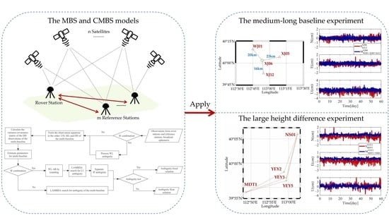
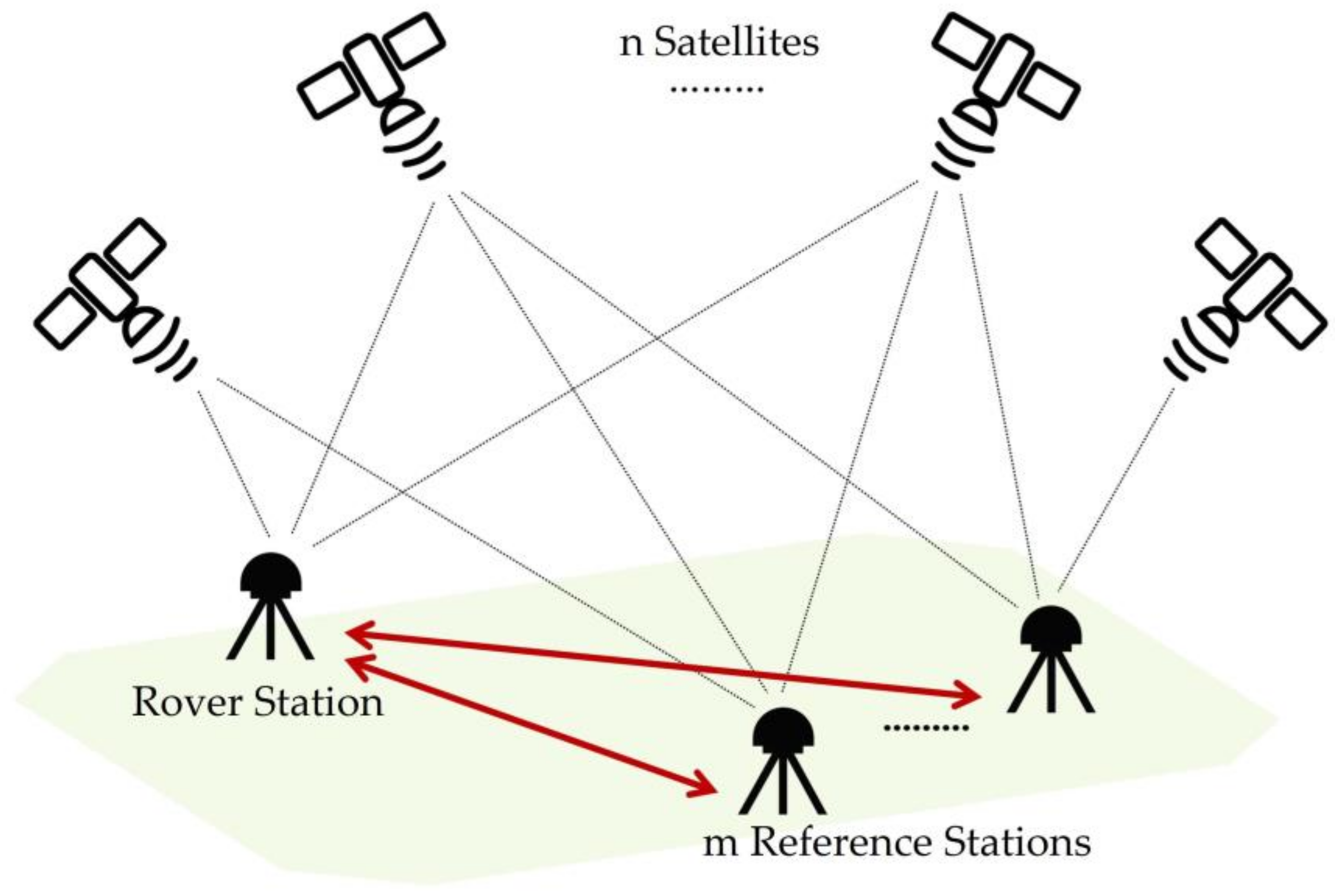
2.1. MBS Mathematical Model

2.1.1. Function Model

As shown in Figure 1, there are $m$ reference stations and one rover station tracking $n$ satellites synchronously, forming $m$ independent baselines. Taking the single-GNSS double-baseline situation as an example, there are $n_j$ and $n_k$ common satellites between the rover station and the $j$-th and $k$-th reference stations, respectively. The carrier phase and code DD observation equations of the epoch $t_i$ can be respectively expressed as:

$$\left\{\begin{array}{l}\lambda \nabla \Delta L_{r{b}_j}^{l_j{q}_j}\left(t_i\right)=\nabla \Delta {\rho }_{r{b}_j}^{l_j{q}_j}\left(t_i\right)-\nabla \Delta I_{r{b}_j}^{l_j{q}_j}\left(t_i\right)+\nabla \Delta T_{r{b}_j}^{l_j{q}_j}\left(t_i\right)+\lambda \nabla \Delta N_{r{b}_j}^{l_j{q}_j}+\nabla \Delta {\epsilon }_{r{b}_j}^{l_j{q}_j}\left(t_i\right)\\ \nabla \Delta P_{r{b}_j}^{l_j{q}_j}\left(t_i\right)=\nabla \Delta {\rho }_{r{b}_j}^{l_j{q}_j}\left(t_i\right)+\nabla \Delta I_{r{b}_j}^{l_j{q}_j}\left(t_i\right)+\nabla \Delta T_{r{b}_j}^{l_{jj}{q}_j}\left(t_i\right)+\nabla \Delta {\delta }_{r{b}_j}^{l_j{q}_j}\left(t_i\right)\\ \lambda \nabla \Delta L_{r{b}_k}^{l_k{q}_k}\left(t_i\right)=\nabla \Delta {\rho }_{r{b}_k}^{l_k{q}_k}\left(t_i\right)-\nabla \Delta I_{r{b}_k}^{l_k{q}_k}\left(t_i\right)+\nabla \Delta T_{r{b}_k}^{l_k{q}_k}\left(t_i\right)+\lambda \nabla \Delta N_{r{b}_k}^{l_k{q}_k}+\nabla \Delta {\epsilon }_{r{b}_k}^{l_k{q}_k}\left(t_i\right)\\ \nabla \Delta P_{r{b}_k}^{l_k{q}_k}\left(t_i\right)=\nabla \Delta {\rho }_{r{b}_k}^{l_k{q}_k}\left(t_i\right)+\nabla \Delta I_{r{b}_k}^{l_k{q}_k}\left(t_i\right)+\nabla \Delta T_{r{b}_k}^{l_k{q}_k}\left(t_i\right)+\nabla \Delta {\delta }_{r{b}_k}^{l_k{q}_k}\left(t_i\right)\end{array}\right.$$

(1)

where $\nabla \Delta$ is the DD operator. $L$ and $P$ represent the carrier phase and code observations, respectively. $l_j$ and $l_k$ are the reference satellites of the $j$-th and $k$-th baselines. $q_j$ and $q_k$ are the common satellites of the $j$-th and $k$-th baselines. $r$ denotes the rover station. $b_{\mathrm{j}}$ and $b_k$ denote the $j$-th and $k$-th reference stations, and $\rho$ denotes the geometric distance between the receiver and the satellite. $I$ denotes ionospheric delay, which is deemed minor enough to be ignored after DD for short baselines, and can be eliminated using a dual-frequency ionosphere-free (IF) linear combination for medium-long baselines. $T$ denotes tropospheric delay, which can be neglected for short baselines, and can be reduced by random walk parameter estimation in the case of medium-long baselines or large height differences. $\lambda$ denotes the wavelength of the carrier phase. $N$ is the phase ambiguity. $\epsilon$ and $\delta$ represent the measurement noise of the carrier phase and code, respectively.

2.1.2. Stochastic Model

The following stochastic model based on the elevation angle is utilized in this study [35]. The variance of the undifferenced (UD) observations can be expressed as:

$${\sigma }^2=a^2+\frac{b^2}{{\mathit{sin}}^2(Ele)}$$

(2)

where represents the variance of UD observations. is the satellite elevation angle. It is assumed that the standard deviation of the code observations is 100 times that of the carrier phase, with for the carrier phase and for the code. The variance-covariance matrices of the UD carrier phase observations of the -th, -th reference station, and the rover station can be expressed as Equation (3).

$$\left\{\begin{array}{c}{R}_{b_j,\phi }=diag{({\sigma }_{{\phi }_{b_j}^{l_j}}^2,\dots ,{\sigma }_{{\phi }_{b_j}^{q_j}}^2)}_{n_j}\\ R_{b_k,\phi }=diag{({\sigma }_{{\phi }_{b_k}^{l_k}}^2,\dots ,{\sigma }_{{\phi }_{b_k}^{q_k}}^2)}_{n_k}\\ R_{r,\phi }=diag{({\sigma }_{{\phi }_r^{l_j}}^2,{\sigma }_{{\phi }_r^{l_k}}^2,\dots ,{\sigma }_{{\phi }_r^{q_{max}}}^2)}_{n_{max}}\end{array}\right.$$

(3)

where and are, respectively, the numbers of the common satellites of the rover station and the -th and -th reference stations. is the total number of common satellites in baselines.

According to the error propagation law, the variance-covariance matrix of the single-differenced (SD) carrier phase observations of baselines can be derived as:

$$R_{rb,\phi }^{Single}={\left[\begin{array}{cccc}{\tilde{E}}_{n_1{n}_{max}}{R}_{r,\phi }{\tilde{E}}_{n_{max}{n}_1}^T+R_{b_{1,\phi }}& {\tilde{E}}_{n_1{n}_{max}}{R}_{r,\phi }{\tilde{E}}_{n_{max}{n}_2}^T& \cdots & {\tilde{E}}_{n_1{n}_{max}}{R}_{r,\phi }{\tilde{E}}_{n_{max}{n}_m}^T\\ {\tilde{E}}_{n_2{n}_{max}}{R}_{r,\phi }{\tilde{E}}_{n_{max}{n}_1}^T& {\tilde{E}}_{n_2{n}_{max}}{R}_{r,\phi }{\tilde{E}}_{n_{max}{n}_2}^T+R_{b_{2,\phi }}& \cdots & {\tilde{E}}_{n_2{n}_{max}}{R}_{r,\phi }{\tilde{E}}_{n_{max}{n}_m}^T\\ ⋮& ⋮& \ddots & ⋮\\ {\tilde{E}}_{n_m{n}_{max}}{R}_{r,\phi }{\tilde{E}}_{n_{max}{n}_1}^T& {\tilde{E}}_{n_m{n}_{max}}{R}_{r,\phi }{\tilde{E}}_{n_{max}{n}_2}^T& \cdots & {\tilde{E}}_{n_m{n}_{max}}{R}_{r,\phi }{\tilde{E}}_{n_{max}{n}_m}^T+R_{b_{m,\phi }}\end{array}\right]}_{m\times m}$$

(4)

where ${\tilde{E}}_{n_i{n}_{max}}$ is the SD operator between stations, $i=1,2,\dots ,j,k,\dots m$.

Equation (4) can be divided into diagonal submatrix ${\tilde{E}}_{n_i{n}_{max}}{R}_{r,\phi }{\tilde{E}}_{n_{max}{n}_i}^T+R_{b_i,\phi }$ and non-diagonal submatrix ${\tilde{E}}_{n_i{n}_{max}}{R}_{r,\phi }{\tilde{E}}_{n_{max}{n}_{i+1}}^T$. The diagonal submatrix can be simplified and expressed as $diag{({\sigma }_{{\phi }_r^{l_j}}^2+{\sigma }_{{\phi }_{b_j}^{l_j}}^2,\dots ,{\sigma }_{{\phi }_r^{q_j}}^2+{\sigma }_{{\phi }_{b_j}^{q_j}}^2)}_{n_j}$, which is equal to the inter-station SD stochastic model of SBS. The non-diagonal submatrix is related to common satellites between baselines, which is essentially the difference between the MBS and SBS stochastic models.

Then the inter-station SD observations of $m$ baselines are differentiated between satellites to obtain DD observations, which are arranged sequentially based on the order of stations. According to the variance-covariance error propagation law, the variance-covariance matrix of DD carrier phase observations can be derived as:

$$R_{rb,\phi }^{Double}=D{R}_{rb,\phi }^{Single}{D}^T$$

(5)

$$\left\{\begin{array}{c}D=diag{\left(D_1,D_2,\dots ,D_m\right)}_{m\times m}\\ D_i={\left[\begin{array}{ccccc}-1& 1& 0& \cdots & 0\\ -1& 0& 1& \cdots & 0\\ ⋮& ⋮& ⋮& \ddots & ⋮\\ -1& 0& 0& \cdots & 1\end{array}\right]}_{\left(n_i-1\right)\times n_i}\end{array}\right.$$

(6)

where $D$ denotes the SD operator between satellites.

2.2. MBS Parameter Estimation

In this section, Kalman filtering (KF) was used for MBS parameter estimation. The main parameters to be estimated included ambiguities and three-dimensional coordinates. Additionally, the correlation between the atmospheric errors of the reference station and the monitoring station decreased as the baseline length or height difference increased. The DD ionospheric and tropospheric residual errors were no longer negligible for baselines with medium-long length or large height difference. Ionospheric delay can be eliminated by using the dual-frequency ionosphere-free (IF) linear combination. The tropospheric delay can be separated into hydrostatic and wet components, with the hydrostatic delay being corrected by a specific model at mm level accuracy [36], whereas the wet delay is more complex and related to the water vapor in the atmosphere, which is difficult to accurately model. Therefore, in this paper, the GPT2_1W surface meteorology model was used to interpolate the station meteorological elements [37], and the hydrostatic delay was corrected using the Saastamoinen model and the Vienna Mapping Function1 (VMF1) mapping function [38]. The relative zenith wet delay (RZWD) between the rover and reference stations has spatial and temporal correlation, thus is estimated as an unknown parameter of a random walk process.

The state vector of the rover station associated with $m$ baselines is:

$$X={[X_r,Y_r,Z_r,RZW{D}_{r{b}_1},\dots ,RZW{D}_{r{b}_m},\Delta \nabla N_{r{b}_1}^{l_1{q}_1},\dots ,,\Delta \nabla N_{r{b}_m}^{l_m{q}_m}]}^T$$

(7)

where $X_r,Y_r,Z_r$ denote the three-dimensional coordinate vector of the rover station. The coordinate components of the rover stations in each baseline should be the same in the same epoch. The SBS model treats them as separate parameters, resulting in several baseline solutions for the same rover station. The MBS model unifies the coordinate parameters of the rover stations in each baseline in data processing and employs only one set of rover station coordinate parameters, considerably increasing the model strength.

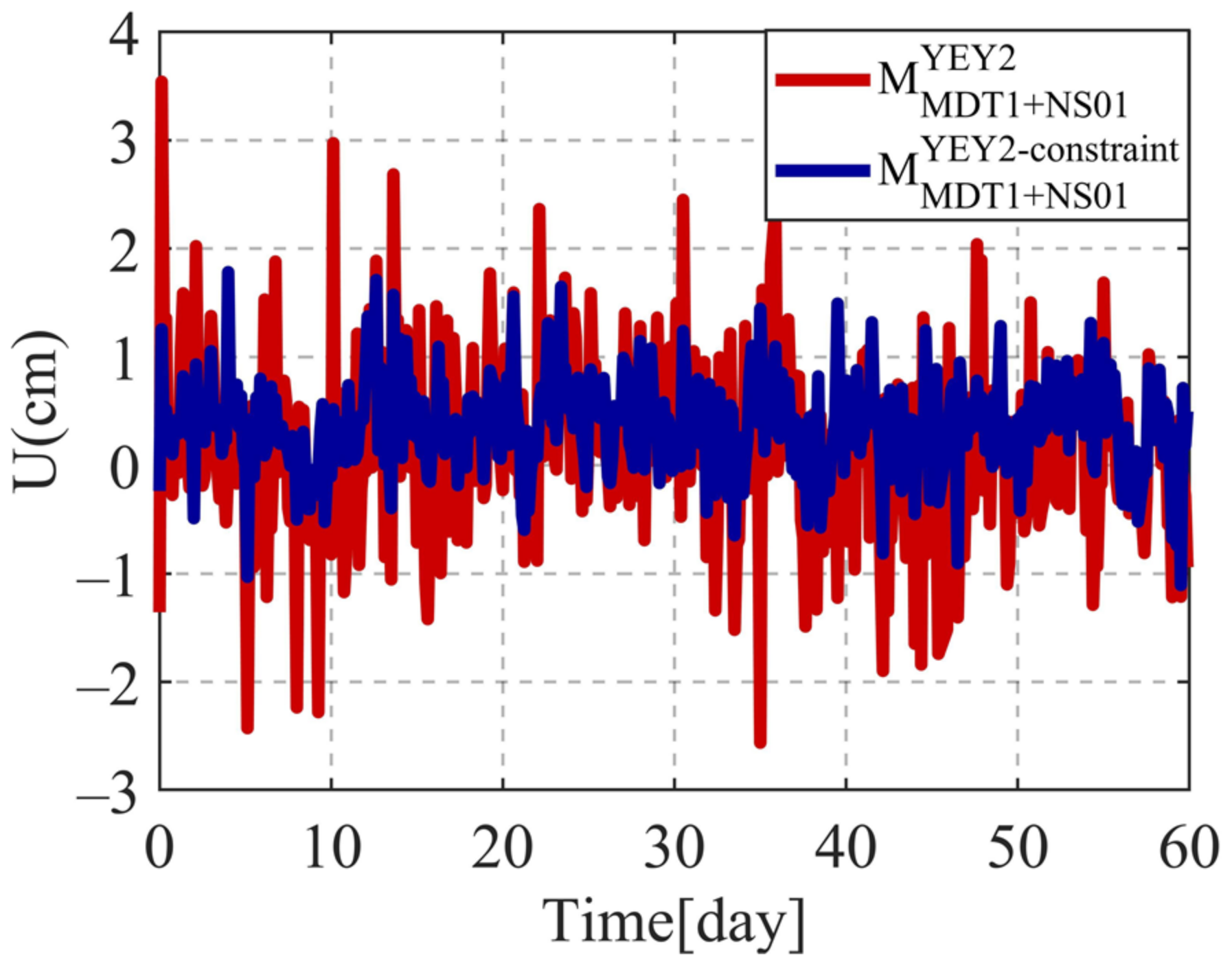
2.3. A Priori Constraint on Tropospheric Delay

The atmospheric delay errors are characterized by spatial and temporal correlation. The relationship between the RZWD and the height difference in the $j$-th and $k$-th baselines is considered to be given by the following formula. The exponential function is used to describe the variation of tropospheric wet delay in the height direction [39,40,41]:

$$\frac{RZW{D}_{r{b}_j}}{e^{k\ast \Delta h_j}}=\frac{RZW{D}_{r{b}_k}}{e^{k\ast \Delta h_k}}$$

(8)

where the value of $k$ is empirically set between $1e^{-5}$ and $1e^{-4}$; $\Delta h_i$ denotes the height difference between the rover station and the $i$-th reference station.

This prior information can be expressed as virtual observations:

$$AX=M$$

(9)

where $X$ is the unknown state vector.

Taking the 1st, 2nd, and 3rd baselines as examples, coefficient matrix $A$ and constant matrix $M$ can be expressed as:

$$A=\left[\begin{array}{ccccccccc}0& 0& 0& 1/e^{k\ast \Delta h_1}& -1/e^{k\ast \Delta h_2}& 0& 0& \dots & 0\\ 0& 0& 0& 1/e^{k\ast \Delta h_1}& 0& -1/e^{k\ast \Delta h_3}& 0& \dots & 0\end{array}\right]$$

(10)

$$M=\left[\begin{array}{c}\left(1/e^{k\ast \Delta h_2}-1/e^{k\ast \Delta h_1}\right)\ast ZW{D}_0\left(r\right)+1/e^{k\ast \Delta h_1}\ast ZW{D}_0\left(b_1\right)-1/e^{k\ast \Delta h_2}\ast ZW{D}_0\left(b_2\right)\\ \left(1/e^{k\ast \Delta h_3}-1/e^{k\ast \Delta h_1}\right)\ast ZW{D}_0\left(r\right)+1/e^{k\ast \Delta h_1}\ast ZW{D}_0\left(b_1\right)-1/e^{k\ast \Delta h_3}\ast ZW{D}_0\left(b_3\right)\end{array}\right]$$

(11)

where $ZW{D}_0$ denotes the wet delay a priori value calculated by the empirical model. The a priori standard deviation (STD) of the virtual observations is empirically set to $0.001 \mathrm{m}$.

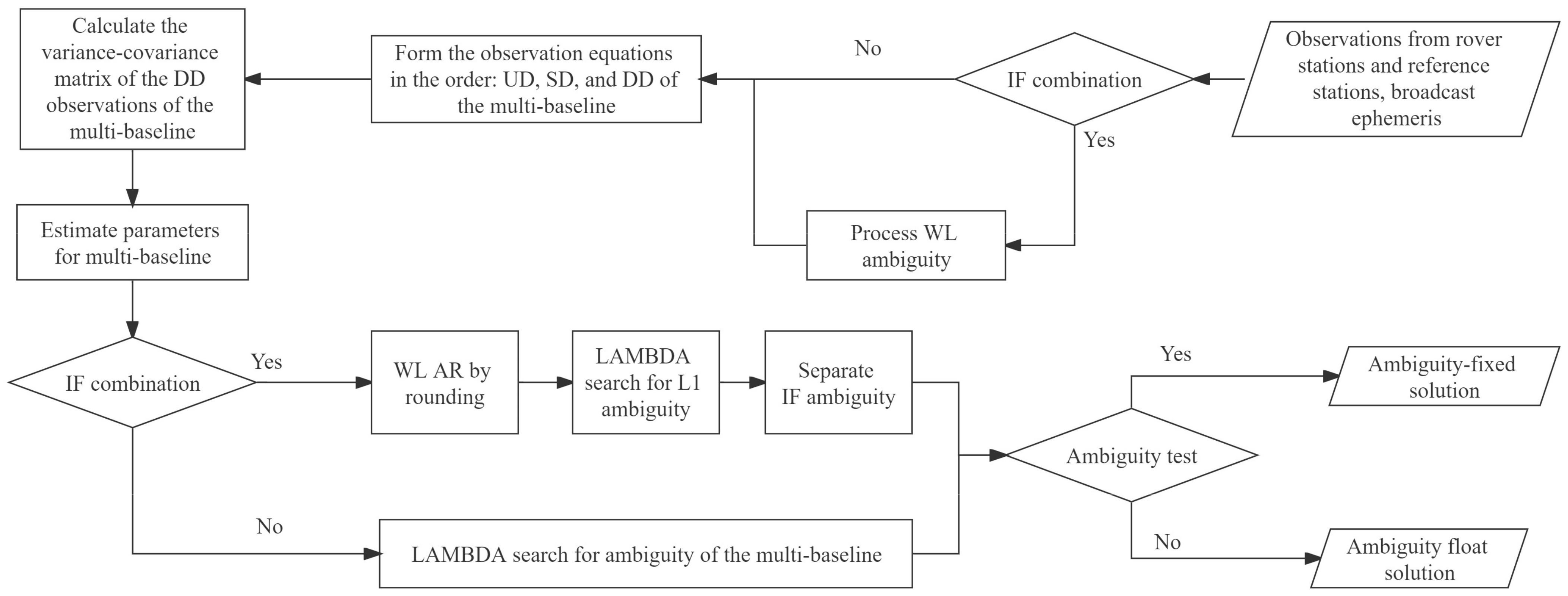
2.4. Data Processing Strategy

Figure 2 depicts the flow chart of the MBS model. A three-step method was used to solve the IF combined AR problem [42]. Firstly, the wide-lane (WL) ambiguity was fixed by rounding, and multi-epoch smoothing was performed using HATCH filtering [43]. Next, the float solution of the IF ambiguity was solved by KF. Then, the L1 ambiguity float solution was extracted from the IF ambiguity using the WL ambiguity, and the Ll ambiguity fixing solution was searched using the well-known LAMBDA method. Finally, the IF ambiguity-fixed solution was obtained.

The observation redundancy is considerably increased by the multi-GNSS MBS compared to the single-GNSS SBS [26]. Using more observations inevitably increases the AR dimension. As the number of AR dimensions increases, the difference in the size of the residual quadratic corresponding to the optimal candidate solution and the suboptimal candidate solution of ambiguity becomes less significant, and the ratio value gets close to 1.0, gradually [44]. Therefore, the commonly adopted empirical threshold of 3.0 is too strict for high-dimension AR, and it is easy to reject the ambiguity that can be fixed correctly. Empirically, the ratio test threshold for the MBS model should be set at 1.3 to 2.5.

3. Experiments and Analysis

In this section, the MBS model was evaluated by conducting experiments using baselines of medium-long lengths and large height differences. The datasets were obtained from an actual ground settlement monitoring project in Shanxi Province, China. Calculations were performed in static mode using a self-developed C++ program.

3.1. Medium-Long Baseline Experiment

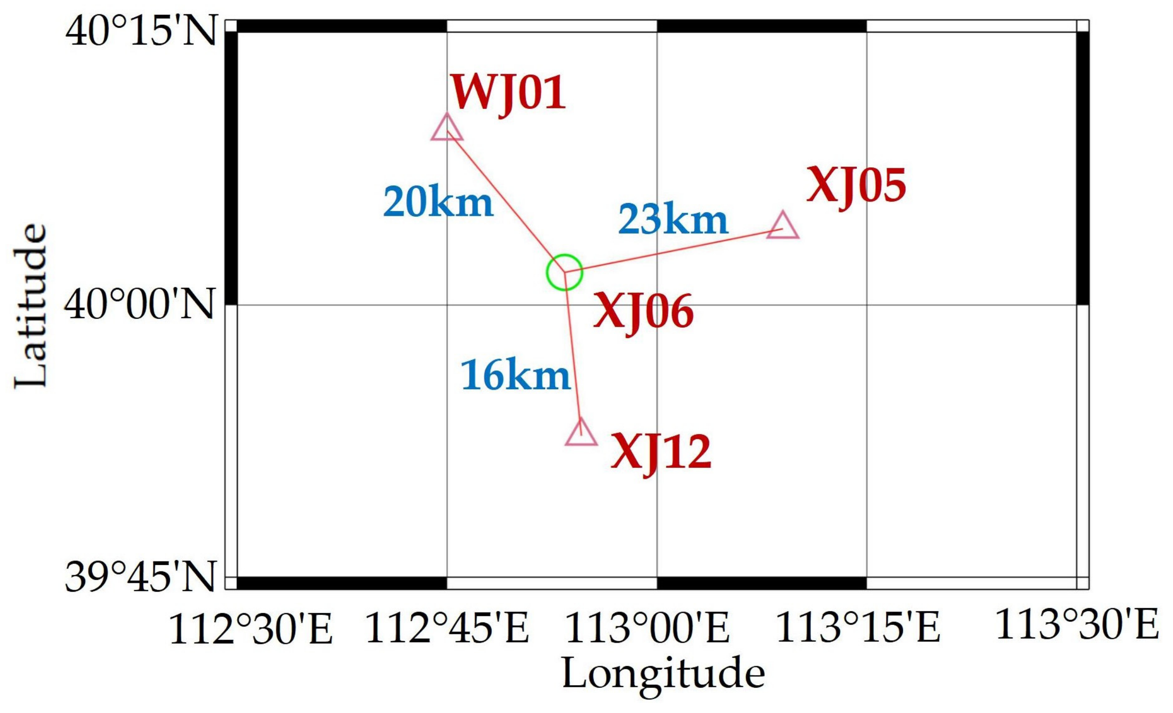
3.1.1. Experimental Design

To compare the positioning performance of the MBS model and SBS model, an ideal monitoring environment was firstly considered. Four relatively stable stations with similar heights were selected. Figure 3 shows the distribution map. The dataset contained dual-frequency GPS observations of 60 days (from 15 February 2020 to 14 April 2020), with a sampling interval of 1 min and a cut-off elevation angle of $15°$. Three independent baselines were formed, using XJ06 as the rover station and XJ12, WJ01, and XJ05 as the reference stations. The approximate lengths were 16, 20, and 23 km, respectively.

Figure 4 shows the position dilution of precision (PDOP) and the number of GPS satellites tracked by the station XJ06 on 15 February 2020. Station XJ06 tracked 5 to 10 GPS satellites with PDOP values oscillating at about 2.3.

Seven data processing strategies with different reference stations were designed and are listed in

Table 1. Medium-long baseline experimental processing strategies.

Strategy	Reference Stations	Rover Station	Model	Baseline Length/km
${\mathrm{S}}_{\mathrm{XJ}12}^{\mathrm{XJ}06}$	XJ12	XJ06	SBS	16
${\mathrm{S}}_{\mathrm{WJ}01}^{\mathrm{XJ}06}$	WJ01	XJ06	SBS	20
${\mathrm{S}}_{\mathrm{XJ}05}^{\mathrm{XJ}06}$	XJ05	XJ06	SBS	23
${\mathrm{M}}_{\mathrm{WJ}01+\mathrm{XJ}12}^{\mathrm{XJ}06}$	WJ01 + XJ12	XJ06	MBS	-
${\mathrm{M}}_{\mathrm{WJ}01+\mathrm{XJ}05}^{\mathrm{XJ}06}$	WJ01 + XJ05	XJ06	MBS	-
${\mathrm{M}}_{\mathrm{XJ}05+\mathrm{XJ}12}^{\mathrm{XJ}06}$	XJ05 + XJ12	XJ06	MBS	-
${\mathrm{M}}_{\mathrm{WJ}01+\mathrm{XJ}05+\mathrm{XJ}12}^{\mathrm{XJ}06}$	WJ01 + XJ05 + XJ12	XJ06	MBS	-

. Strategies ${\mathrm{S}}_{\mathrm{XJ}12}^{\mathrm{XJ}06}$, ${\mathrm{S}}_{\mathrm{WJ}01}^{\mathrm{XJ}06}$ and ${\mathrm{S}}_{\mathrm{XJ}05}^{\mathrm{XJ}06}$ used the SBS model, with the reference stations being XJ12, WJ01 and XJ05 respectively. Strategies ${\mathrm{M}}_{\mathrm{WJ}01+\mathrm{XJ}12}^{\mathrm{XJ}06}$, ${\mathrm{M}}_{\mathrm{WJ}01+\mathrm{XJ}05}^{\mathrm{XJ}06}$ and ${\mathrm{M}}_{\mathrm{XJ}05+\mathrm{XJ}12}^{\mathrm{XJ}06}$ adopted the MBS model with double reference stations (namely, WJ01 + XJ12, WJ01 + XJ05, and XJ05 + XJ12). Strategy ${\mathrm{M}}_{\mathrm{WJ}01+\mathrm{XJ}05+\mathrm{XJ}12}^{\mathrm{XJ}06}$ adopted the MBS model using triple reference stations. It was used to check whether simply increasing the number of reference stations could have a positive impact on the positioning. GPS L1/L2 IF combination was used to eliminate ionospheric effect, and the empirical tropospheric model Saastamoinen was used to reduce the effect of tropospheric delay error. The length of static solution was 2 h. Daily static solutions were determined using software Bernese 5.0 as the true values.

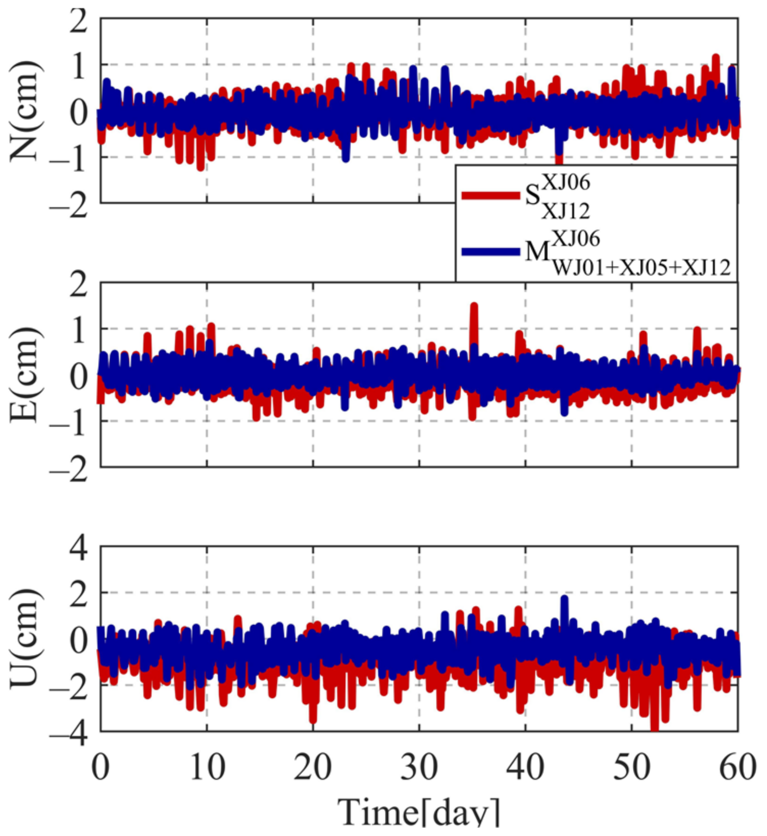
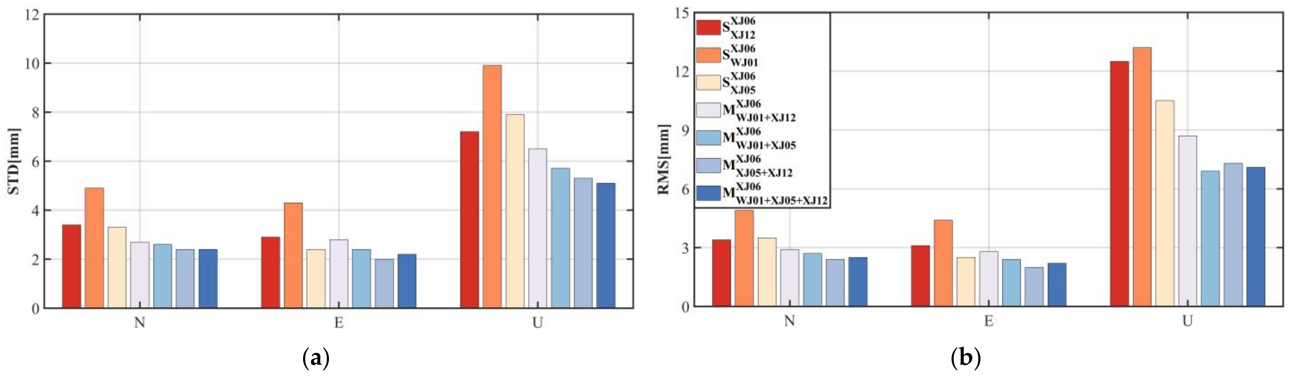
3.1.2. Analysis of Monitoring Accuracy for Different Reference Stations

Figure 5 shows the baseline positioning errors of ${\mathrm{S}}_{\mathrm{XJ}12}^{\mathrm{XJ}06}$ and ${\mathrm{M}}_{\mathrm{WJ}01+\mathrm{XJ}05+\mathrm{XJ}12}^{\mathrm{XJ}06}$.Figure 6 shows the STD and root-mean-square (RMS) values of the positioning errors for the seven processing strategies in the north (N), east (E), and up (U) components. The corresponding statistics are listed in

Table 2. The positioning error statistics for SBS and MBS processing strategies with different reference stations at rover station XJ06.

Strategy	STD/mm			Improvement/%			RMS/mm			Improvement/%
	N	E	U	N	E	U	N	E	U	N	E	U
${\mathrm{S}}_{\mathrm{XJ}12}^{\mathrm{XJ}06}$	3.4	2.9	7.2	-	-	-	3.4	3.1	12.5	-	-	-
${\mathrm{S}}_{\mathrm{WJ}01}^{\mathrm{XJ}06}$	4.9	4.3	9.9	-	-	-	4.9	4.4	13.2	-	-	-
${\mathrm{S}}_{\mathrm{XJ}05}^{\mathrm{XJ}06}$	3.3	2.4	7.9	-	-	-	3.5	2.5	10.5	-	-	-
${\mathrm{M}}_{\mathrm{WJ}01+\mathrm{XJ}12}^{\mathrm{XJ}06}$	2.7	2.8	6.5	20.6	3.5	9.7	2.9	2.8	8.7	14.7	9.7	30.4
${\mathrm{M}}_{\mathrm{WJ}01+\mathrm{XJ}05}^{\mathrm{XJ}06}$	2.6	2.4	5.7	23.5	17.2	20.8	2.7	2.4	6.9	20.6	22.6	44.8
${\mathrm{M}}_{\mathrm{XJ}05+\mathrm{XJ}12}^{\mathrm{XJ}06}$	2.4	2.0	5.3	29.4	31.0	26.4	2.4	2.0	7.3	29.4	35.5	41.6
${\mathrm{M}}_{\mathrm{WJ}01+\mathrm{XJ}05+\mathrm{XJ}12}^{\mathrm{XJ}06}$	2.4	2.2	5.1	29.4	24.1	29.2	2.5	2.2	7.1	26.5	29.0	43.2
Average improvement rate	-	-	-	25.7	19.0	21.5	-	-		22.8	24.2	40.0

, where the improvement rate of the MBS strategy was calculated compared to the SBS strategy ${\mathrm{S}}_{\mathrm{XJ}12}^{\mathrm{XJ}06}$ with the shortest baseline length. From Figure 5, it can be seen that the positioning error fluctuation of strategy ${\mathrm{M}}_{\mathrm{WJ}01+\mathrm{XJ}05+\mathrm{XJ}12}^{\mathrm{XJ}06}$ was significantly smaller than that of SBS strategy ${\mathrm{S}}_{\mathrm{XJ}12}^{\mathrm{XJ}06}$, which fluctuated in the N/E/U direction within about 1/1/2 cm, and the rest of the strategies had similar results. The experimental results showed that the positioning accuracy of the MBS model was higher than that of the SBS model. The average improvement of coordinate STD values of the MBS model was approximately 25.7, 19.0, and 21.5% in the N, E, and U components, respectively, with the maximum improvement of about 31.0%. The average improvement of the RMS values was about 22.8, 24.2, and 40.0% in the N, E, and U components, respectively, with a maximum improvement of about 44.8%.

It was also clear that the improvement rate of the positioning results was related to the quality of baselines involved in the MBS solution. Most notably, the positioning accuracy of strategy ${\mathrm{M}}_{\mathrm{WJ}01+\mathrm{XJ}05}^{\mathrm{XJ}06}$ was better than that of the single-baseline strategy. It indicates that in actual deformation monitoring, if one cannot select a reference station in the near distance, a higher positioning accuracy can still be achieved by using the MBS model to combined several distant reference stations.

The positioning accuracy of the triple-baseline strategy was generally better than that of the double-baseline strategy, indicating that increasing the number of reference stations benefits the positioning due to an increased observation redundancy. However, the difference of positioning accuracy between strategy ${\mathrm{M}}_{\mathrm{WJ}01+\mathrm{XJ}05+\mathrm{XJ}12}^{\mathrm{XJ}06}$ and strategy ${\mathrm{M}}_{\mathrm{XJ}05+\mathrm{XJ}12}^{\mathrm{XJ}06}$ was small. This is probably because strategy ${\mathrm{M}}_{\mathrm{WJ}01+\mathrm{XJ}05+\mathrm{XJ}12}^{\mathrm{XJ}06}$ included baseline WJ01-XJ06, whose quality was the worst of the three baselines as shown in the single-baseline strategy results (see Table 2).

3.2. Large Height Difference Experiment

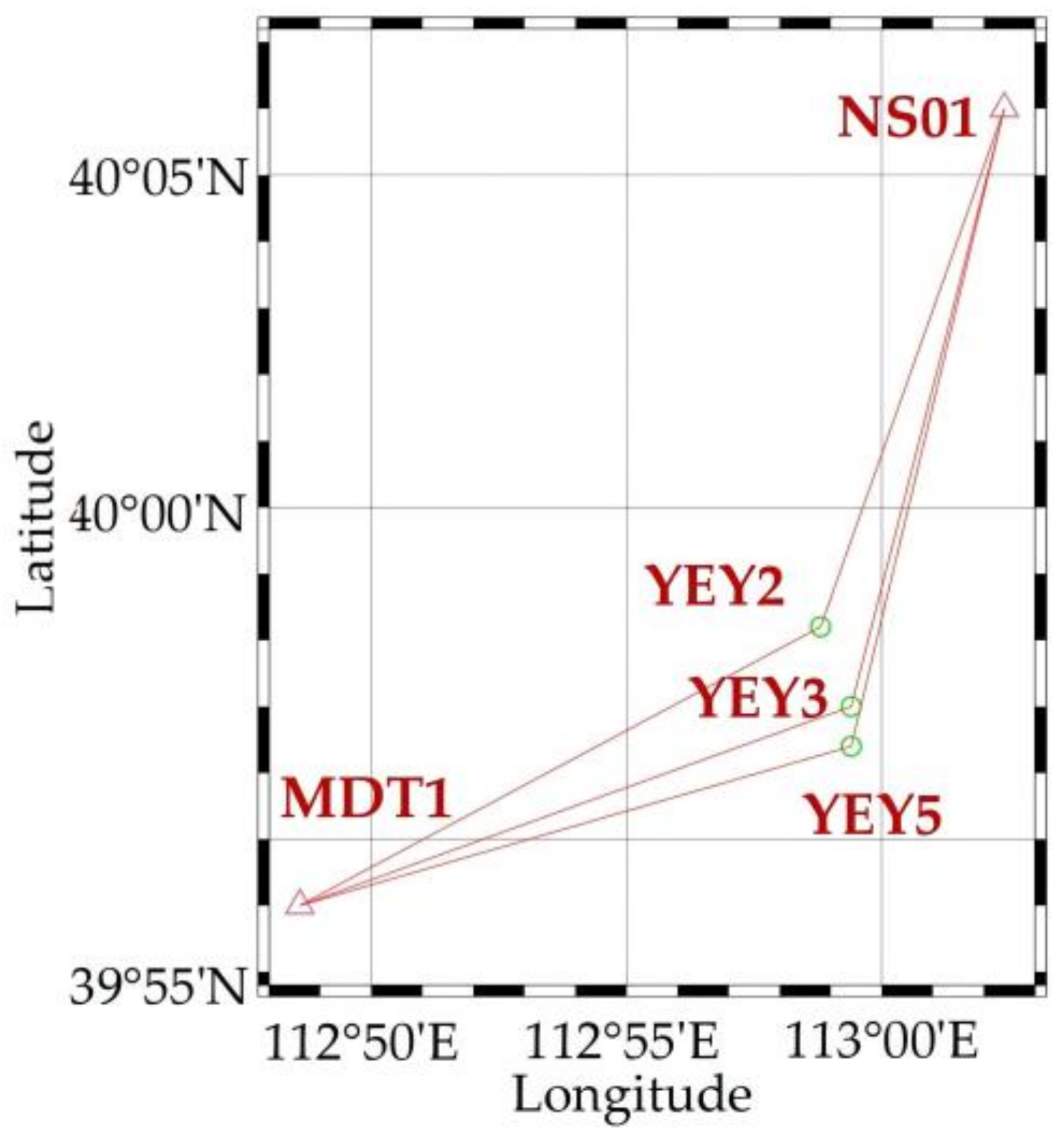
3.2.1. Experimental Design

Three monitoring stations (YEY2, YEY3, YEY5) equipped with single-frequency receivers in the ground settlement project were selected to analyze the positioning performance of the proposed MBS model in monitoring baselines with large height differences. Six independent baselines with different height differences were formed with two reference stations (MDT1, NS01). From the rover to reference stations, the baseline lengths were about 15 km and the height differences were about 200 m. Figure 7 shows the distribution map of the stations. The datasets were collected continuously for 60 days, from 15 February 2020 to 14 April 2020, with a sampling interval of 30 s and a satellite cut-off elevation angle of $15°$. Figure 8 shows the number of visible satellites and PDOPs of station YEY2 on 15 February 2020. In this contribution, G and C stand for GPS and BDS respectively, PDOP.G and PDOP.C are PDOPs for GPS and BDS. It can be seen that the average number of visible satellites for the combined GPS/BDS reached 17, while the number of GPS satellites was only about 7. The PDOP values for GPS/BDS were significantly smaller than those of GPS-only and BDS-only solutions, indicating that combining GPS/BDS observations enhances the satellite visibility.

Table 3. Large height difference experimental processing strategies.

Strategy	Reference Stations	Rover Station	Height Differences w.r.t. Reference Stations/m	Model	Tropospheric Constraint
${\mathrm{S}}_{\mathrm{MDT}1}^{\mathrm{YEY}2}$	MDT1	YEY2	263	SBS	No
${\mathrm{S}}_{\mathrm{MDT}1}^{\mathrm{YEY}3}$	MDT1	YEY3	200	SBS	No
${\mathrm{S}}_{\mathrm{MDT}1}^{\mathrm{YEY}5}$	MDT1	YEY5	112	SBS	No
${\mathrm{M}}_{\mathrm{MDT}1+\mathrm{NS}01}^{\mathrm{YEY}2\left(\mathrm{G}\right)}$	MDT1 + NS01	YEY2	(263, 152)	MBS	No
${\mathrm{M}}_{\mathrm{MDT}1+\mathrm{NS}01}^{\mathrm{YEY}2\left(\mathrm{C}\right)}$	MDT1 + NS01	YEY2	(263, 152)	MBS	No
${\mathrm{M}}_{\mathrm{MDT}1+\mathrm{NS}01}^{\mathrm{YEY}2}$	MDT1 + NS01	YEY2	(263, 152)	MBS	No
${\mathrm{M}}_{\mathrm{MDT}1+\mathrm{NS}01}^{\mathrm{YEY}2-\mathrm{constraint}}$	MDT1 + NS01	YEY2	(263, 152)	CMBS	Yes
${\mathrm{M}}_{\mathrm{MDT}1+\mathrm{NS}01}^{\mathrm{YEY}3}$	MDT1 + NS01	YEY3	(200, 215)	MBS	No
${\mathrm{M}}_{\mathrm{MDT}1+\mathrm{NS}01}^{\mathrm{YEY}3-\mathrm{constraint}}$	MDT1 + NS01	YEY3	(200, 215)	CMBS	Yes
${\mathrm{M}}_{\mathrm{MDT}1+\mathrm{NS}01}^{\mathrm{YEY}5}$	MDT1 + NS01	YEY5	(112, 303)	MBS	No
${\mathrm{M}}_{\mathrm{MDT}1+\mathrm{NS}01}^{\mathrm{YEY}5-\mathrm{constraint}}$	MDT1 + NS01	YEY5	(112, 303)	CMBS	Yes

lists eleven strategies to compare the positioning performance of SBS strategies (e.g., ${\mathrm{S}}_{\mathrm{MDT}1}^{\mathrm{YEY}2}$), single-GNSS strategies (${\mathrm{M}}_{\mathrm{MDT}1+\mathrm{NS}01}^{\mathrm{YEY}2\left(\mathrm{G}\right)}$ and ${\mathrm{M}}_{\mathrm{MDT}1+\mathrm{NS}01}^{\mathrm{YEY}2\left(\mathrm{C}\right)}$ that respectively using GPS-only and BDS-only observations), MBS strategies (e.g., ${\mathrm{M}}_{\mathrm{MDT}1+\mathrm{NS}01}^{\mathrm{YEY}2}$) and corresponding CMBS strategies (e.g., ${\mathrm{M}}_{\mathrm{MDT}1+\mathrm{NS}01}^{\mathrm{YEY}2-\mathrm{constraint}}$). The session length was 3 h. The reference coordinates of each station were obtained in the same way as introduced in Section 3.1. Table 3 also shows the height difference between the rover station and each reference station. For example, (263 m, 152 m) in strategy ${\mathrm{M}}_{\mathrm{MDT}1+\mathrm{NS}01}^{\mathrm{YEY}2}$ indicates that the height differences between reference stations MDT1 and NS01 and rover station YEY2 were 263 and 152 m, respectively.

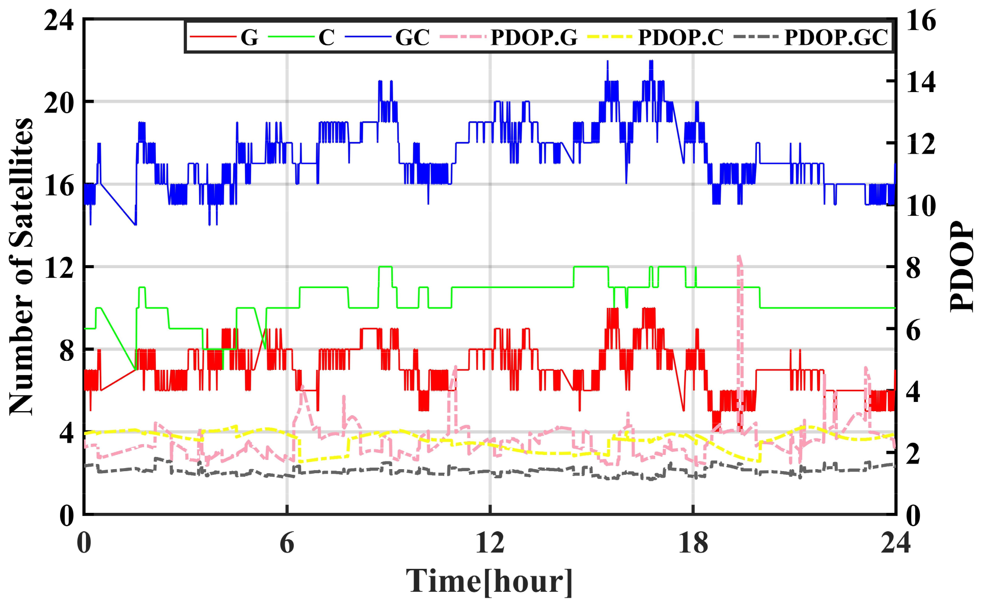
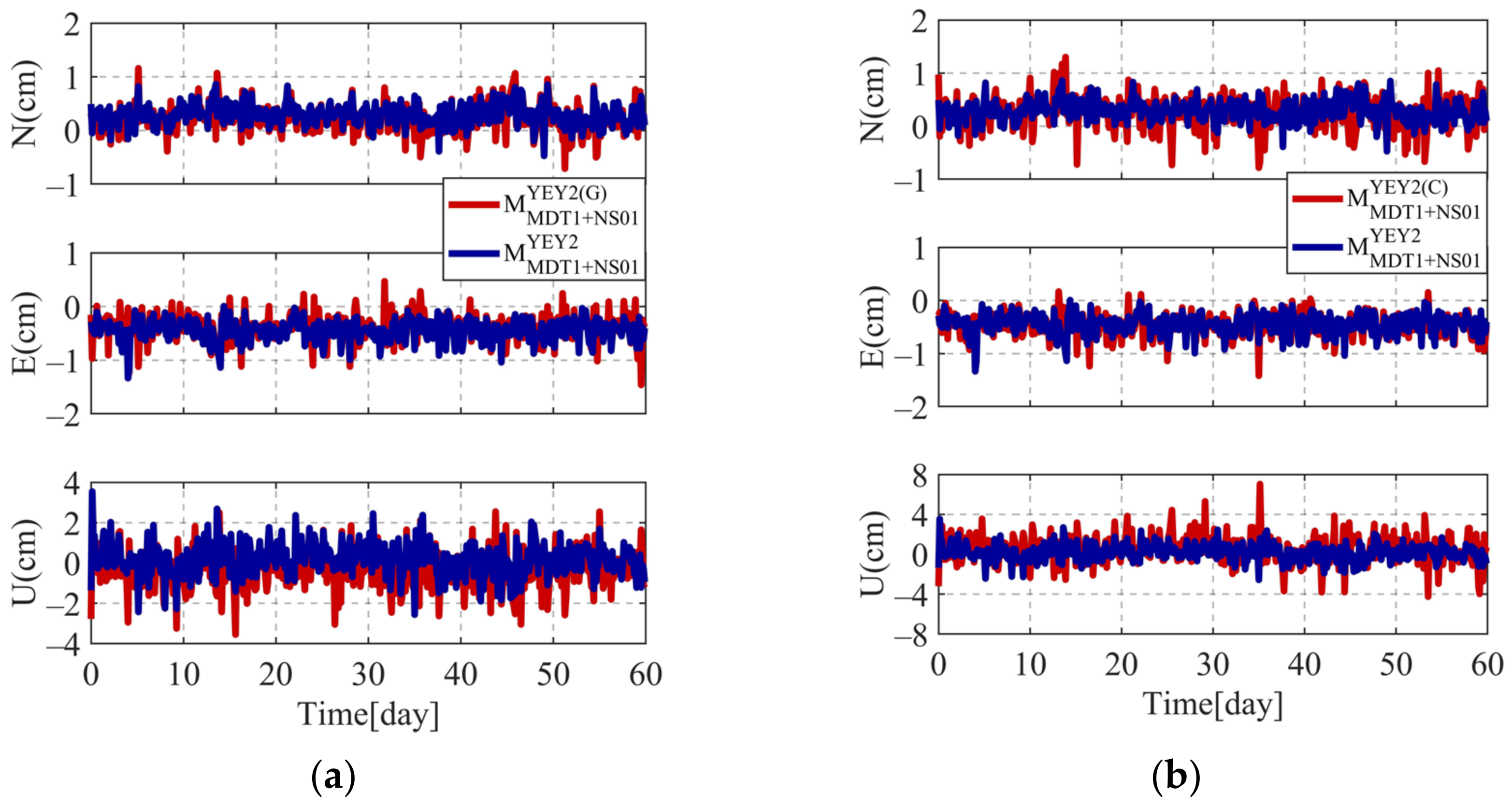
3.2.2. Analysis of Monitoring Accuracy for Different Satellite Systems

Figure 9 presents the positioning errors of YEY2 in N, E, and U components of SBS processing strategies ${\mathrm{M}}_{\mathrm{MDT}1+\mathrm{NS}01}^{\mathrm{YEY}2\left(\mathrm{G}\right)}$, ${\mathrm{M}}_{\mathrm{MDT}1+\mathrm{NS}01}^{\mathrm{YEY}2\left(\mathrm{C}\right)}$ and ${\mathrm{M}}_{\mathrm{MDT}1+\mathrm{NS}01}^{\mathrm{YEY}2}$, and the corresponding statistics are listed in

Table 4. The positioning error statistics of single-GNSS and dual-GNSS strategies.

Strategy	STD/mm			Improvement/%			RMS/mm			Improvement/%
	N	E	U	N	E	U	N	E	U	N	E	U
${\mathrm{M}}_{\mathrm{MDT}1+\mathrm{NS}01}^{\mathrm{YEY}2\left(\mathrm{G}\right)}$	2.6	2.5	9.8	-	-	-	3.4	4.7	10.4	-	-	-
${\mathrm{M}}_{\mathrm{MDT}1+\mathrm{NS}01}^{\mathrm{YEY}2\left(\mathrm{C}\right)}$	3.0	2.2	13.7	-	-	-	4.1	5.2	14.4	-	-	-
${\mathrm{M}}_{\mathrm{MDT}1+\mathrm{NS}01}^{\mathrm{YEY}2}$	2.0	1.9	8.0	23.1	24.0	18.4	3.5	4.8	8.1	$-$2.9	$-$2.1	22.1

. The experimental results showed that the positioning accuracy of the combined GPS/BDS solutions was superior to those of GPS-only and BDS-only solutions. Compared with the GPS-only solution, the improvement rates of the STD values of the combined GPS/BDS were approximately 23.1, 24.0, and 18.4% in the N, E, and U components, respectively, and the improvement of the RMS values in the U component was more significant than the horizontal components. Compared with the BDS-only solution, the improvement rates of the STD values of the combined GPS/BDS were about 33.3, 13.6, and 41.6% in the N, E, and U components, respectively, and the improvement rates of the RMS values were about 14.6, 7.7, and 43.8% in the N, E, and U components, respectively.

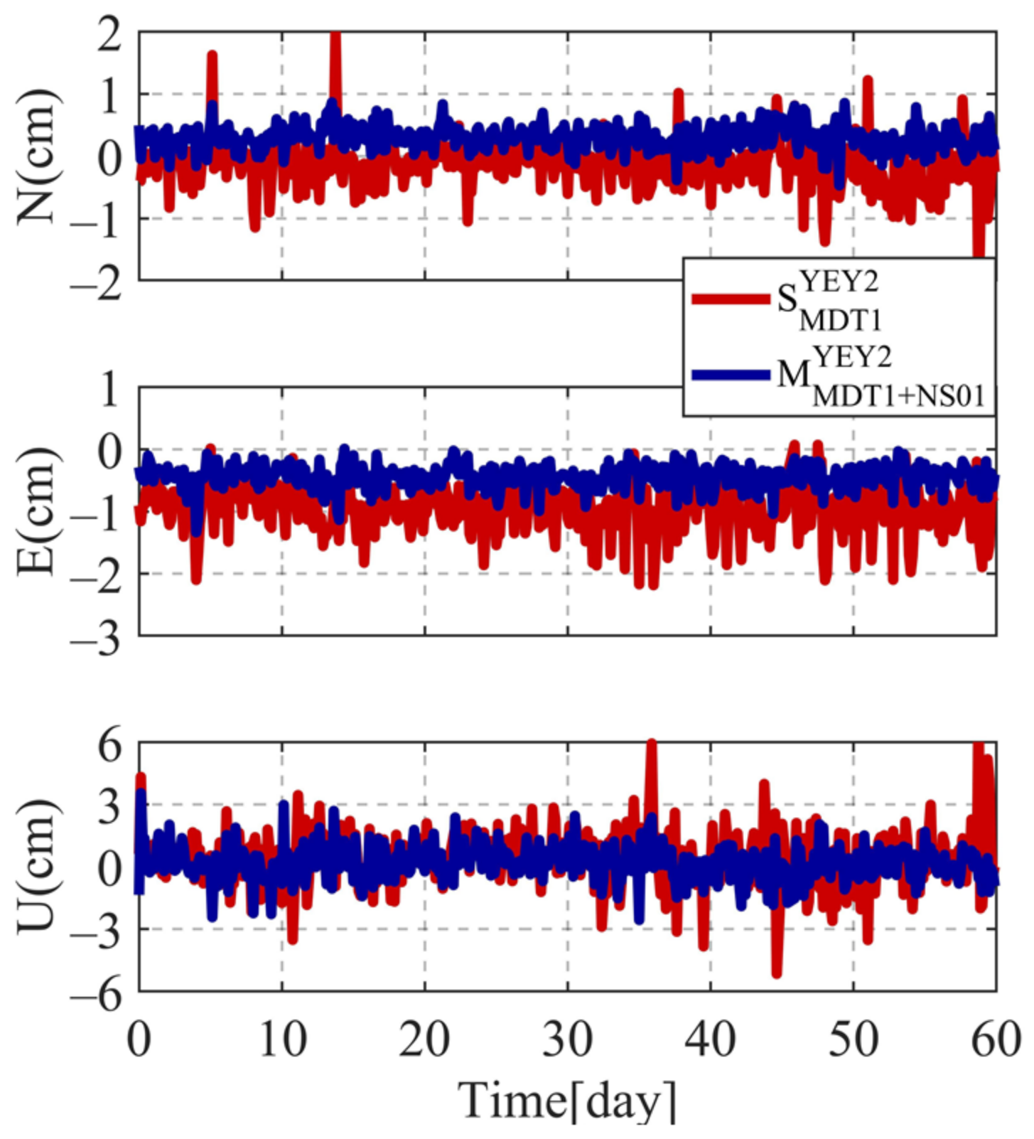
3.2.3. Analysis of Monitoring Accuracy for Large Height Difference

Figure 10 shows the positioning errors at YEY2 station when using processing strategies ${\mathrm{S}}_{\mathrm{MDT}1}^{\mathrm{YEY}2}$ and ${\mathrm{M}}_{\mathrm{MDT}1+\mathrm{NS}01}^{\mathrm{YEY}2}$.

Table 5. The positioning error statistics of SBS, MBS and CMBS processing strategies with different height differences.

Strategy	STD/mm			Improvement/%			RMS/mm			Improvement/%
	N	E	U	N	E	U	N	E	U	N	E	U
${\mathrm{S}}_{\mathrm{MDT}1}^{\mathrm{YEY}2}$	3.8	3.9	13.0	-	-	-	4.1	10.4	13.7	-	-	-
${\mathrm{S}}_{\mathrm{MDT}1}^{\mathrm{YEY}3}$	3.4	4.4	13.8	-	-	-	5.1	12.0	14.4	-	-	-
${\mathrm{S}}_{\mathrm{MDT}1}^{\mathrm{YEY}5}$	3.6	4.6	13.2	-	-	-	12.2	9.1	13.3	-	-	-
${\mathrm{M}}_{\mathrm{MDT}1+\mathrm{NS}01}^{\mathrm{YEY}2}$	2.0	1.9	8.0	47.4	51.3	38.5	3.5	4.8	8.1	14.6	53.9	40.9
${\mathrm{M}}_{\mathrm{MDT}1+\mathrm{NS}01}^{\mathrm{YEY}2-\mathrm{constraint}}$	2.0	1.9	4.4	47.4	51.3	66.2	3.4	4.8	5.7	17.1	53.9	58.4
${\mathrm{M}}_{\mathrm{MDT}1+\mathrm{NS}01}^{\mathrm{YEY}3}$	2.1	2.2	8.6	38.2	50.0	37.7	2.2	6.4	10.9	56.9	46.7	24.3
${\mathrm{M}}_{\mathrm{MDT}1+\mathrm{NS}01}^{\mathrm{YEY}3-\mathrm{constraint}}$	2.1	2.2	5.6	38.2	50.0	59.4	2.2	6.4	9.8	56.9	46.7	31.9
${\mathrm{M}}_{\mathrm{MDT}1+\mathrm{NS}01}^{\mathrm{YEY}5}$	2.3	2.6	8.8	36.1	43.5	33.3	7.6	3.6	10.2	37.7	60.4	23.3
${\mathrm{M}}_{\mathrm{MDT}1+\mathrm{NS}01}^{\mathrm{YEY}5-\mathrm{constraint}}$	2.3	2.6	8.8	36.1	43.5	33.3	7.6	3.6	10.2	37.7	60.4	23.3
Average improvement rate	-	-	-	40.6	48.3	44.7	-	-	-	36.8	53.7	33.7

lists the STD and RMS values of the nine strategies, as well as the improvement rates of six MBS strategies in comparison to single-baseline strategies. The results show that the positioning errors of the MBS and CMBS models were smaller than those of the SBS model. The average performance improvement of STD values of the MBS and CMBS models was about 40.6, 48.3, and 44.7% in the N, E, and U components, respectively, with a maximum improvement rate of 66.2%. The average improvement rate of RMS values was about 36.8, 53.7, and 33.7% in the N, E, and U components, respectively, with a maximum improvement rate of 60.4%. Thus, in the deformation monitoring environment with large height differences, the proposed MBS and CMBS models could have superior positioning performance to the SBS model.

Figure 11 shows the positioning errors of strategies ${\mathrm{M}}_{\mathrm{MDT}1+\mathrm{NS}01}^{\mathrm{YEY}2}$ and ${\mathrm{M}}_{\mathrm{MDT}1+\mathrm{NS}01}^{\mathrm{YEY}2-\mathrm{constraint}}$ in the U component. The STD and RMS values in the U component of the six strategies are listed in

Table 6. The positioning error of MBS and CMBS processing strategies in the U component.

Strategy	STD/mm	Improvement/%	RMS/mm	Improvement/%
${\mathrm{M}}_{\mathrm{MDT}1+\mathrm{NS}01}^{\mathrm{YEY}2}$	8.0	-	8.1	-
${\mathrm{M}}_{\mathrm{MDT}1+\mathrm{NS}01}^{\mathrm{YEY}2-\mathrm{constraint}}$	4.4	45.0	5.7	29.6
${\mathrm{M}}_{\mathrm{MDT}1+\mathrm{NS}01}^{\mathrm{YEY}3}$	8.6	-	10.9	-
${\mathrm{M}}_{\mathrm{MDT}1+\mathrm{NS}01}^{\mathrm{YEY}3-\mathrm{constraint}}$	5.6	34.9	9.8	10.1
${\mathrm{M}}_{\mathrm{MDT}1+\mathrm{NS}01}^{\mathrm{YEY}5}$	8.8	-	10.2	-
${\mathrm{M}}_{\mathrm{MDT}1+\mathrm{NS}01}^{\mathrm{YEY}5-\mathrm{constraint}}$	8.8	0.0	10.2	0.0

. It can be seen that the positioning accuracy of the CMBS model was higher than that of the MBS model, with a maximum improvement of 45.0% for STD values and 29.6% for RMS values. Therefore, the CMBS model could improve the positioning accuracy in the U direction in the deformation monitoring environment with large height differences.

4. Conclusions

The existing GNSS deformation monitoring systems often use the SBS model, which ignores baseline correlation and has limited positioning accuracy when processing baselines with medium-long lengths or large height differences. In this study, we constructed a multi-baseline mathematical model based on DD observation equations and adopted a multi-baseline tropospheric delay estimation method based on a priori constraints on the tropospheric delay parameters.

Datasets from baselines with medium-long lengths and large height differences were used to verify the feasibility of the proposed MBS model, and the following conclusions were obtained from the results:

• For baselines with medium-long lengths and large height differences, the proposed MBS model can provide better monitoring performance than the SBS model. Compared with the SBS model, the MBS model can improve the positioning accuracy of medium-long baselines with an average improvement of about (25.7/19.0/21.5%) and (22.8/24.2/40.0%) in the N/E/U components, with the highest improvement of about (29.4/31.0/29.2%) and (29.4/35.5/44.8%) in the N/E/U components, respectively. For baselines with large height differences, compared with the SBS model, the MBS model can improve the positioning accuracy with an average improvement of about (40.6/48.3/44.7%) and (36.8/53.7/33.7%) in the N/E/U components, with the highest improvement of about (47.4/51.3/66.2%) and (56.9/60.4/58.4%) in the N/E/U components, respectively. The MBS model uses multiple reference stations thus can improve the positioning model strength and observation redundancy. This is especially beneficial for applying GNSS in complex monitoring environments such as canyons, open pits, slopes, large-area ground settlement, and long-spanned bridges and railroads.
• The accuracy of the MBS model is related to the number of reference stations and the quality of the baselines. With comparable baseline quality, the accuracy of the MBS model improves as the number of reference stations increases. Medium-long baseline experimental results show that compared with the SBS model, the MBS model using double reference stations can achieve an average improvement rate of about 24.0%, while the MBS model using triple reference stations can achieve an average improvement rate of about 30.2%.
• Compared with GPS-only and BDS-only positioning, the combined GPS/BDS positioning has an accuracy improvement of an average of 13.8 and 25.8% in the baseline components. Meanwhile, the proposed CMBS model can improve accuracy in the U direction and reach up to 45.0%.

Future research will be focused on the application of the MBS approach to near-real-time dynamic monitoring. Baselines with larger tropospheric residual errors will be further investigated.

References

1. Yu, W.; Peng, H.; Pan, L.; Dai, W.; Qu, X.; Ren, Z. Performance Assessment of High-Rate GPS/BDS Precise Point Positioning for Vibration Monitoring Based on Shaking Table Tests. Adv. Space Res. 2022, 69, 2362–2375. [Google Scholar] [CrossRef]
2. Yan, H.; Dai, W.; Xie, L.; Xu, W. Fusion of GNSS and InSAR Time Series Using the Improved STRE Model: Applications to the San Francisco Bay Area and Southern California. J. Geod. 2022, 96, 47. [Google Scholar] [CrossRef]
3. Shen, N.; Chen, L.; Liu, J.; Wang, L.; Tao, T.; Wu, D.; Chen, R. A Review of Global Navigation Satellite System (GNSS)-Based Dynamic Monitoring Technologies for Structural Health Monitoring. Remote Sens. 2019, 11, 1001. [Google Scholar] [CrossRef] [Green Version]
4. Zhong, P.; Ding, X.; Yuan, L.; Xu, Y.; Kwok, K.; Chen, Y. Sidereal Filtering Based on Single Differences for Mitigating GPS Multipath Effects on Short Baselines. J. Geod. 2010, 84, 145–158. [Google Scholar] [CrossRef]
5. Dai, W.; Huang, D.; Cai, C. Multipath Mitigation via Component Analysis Methods for GPS Dynamic Deformation Monitoring. GPS Solut. 2014, 18, 417–428. [Google Scholar] [CrossRef]
6. Chen, J.; Yue, D.; Liu, Z.; Xu, C.; Zhu, S.; Chen, H. Experimental Research on Daily Deformation Monitoring of Bridge Using BDS/GPS. Surv. Rev. 2019, 51, 472–482. [Google Scholar] [CrossRef]
7. Msaewe, H.A.; Hancock, C.M.; Psimoulis, P.A.; Roberts, G.W.; Bonenberg, L.; de Ligt, H. Investigating Multi-GNSS Performance in the UK and China Based on a Zero-Baseline Measurement Approach. Measurement 2017, 102, 186–199. [Google Scholar] [CrossRef]
8. Quan, Y.; Lau, L.; Roberts, G.W.; Meng, X. Measurement Signal Quality Assessment on All Available and New Signals of Multi-GNSS (GPS, GLONASS, Galileo, BDS, and QZSS) with Real Data. J. Navig. 2016, 69, 313–334. [Google Scholar] [CrossRef] [Green Version]
9. Roberts, G.W.; Tang, X. The Use of PSD Analysis on BeiDou and GPS 10 Hz Dynamic Data for Change Detection. Adv. Space Res. 2017, 59, 2794–2808. [Google Scholar] [CrossRef] [Green Version]
10. Huang, G.; Du, Y.; Meng, L.; Huang, G.; Wang, J.; Han, J. Application Performance Analysis of Three GNSS Precise Positioning Technology in Landslide Monitoring. In China Satellite Navigation Conference (CSNC) 2017 Proceedings: Volume I; Sun, J., Liu, J., Yang, Y., Fan, S., Yu, W., Eds.; Lecture Notes in Electrical Engineering; Springer: Singapore, 2017; Volume 437, pp. 139–150. ISBN 978-981-10-4587-5. [Google Scholar]
11. Xi, R.; Chen, H.; Meng, X.; Jiang, W.; Chen, Q. Reliable Dynamic Monitoring of Bridges with Integrated GPS and BeiDou. J. Surv. Eng. 2018, 144, 04018008. [Google Scholar] [CrossRef]
12. Li, B.; Shen, Y.; Feng, Y.; Gao, W.; Yang, L. GNSS Ambiguity Resolution with Controllable Failure Rate for Long Baseline Network RTK. J. Geod. 2014, 88, 99–112. [Google Scholar] [CrossRef]
13. Wilgan, K.; Hurter, F.; Geiger, A.; Rohm, W.; Bosy, J. Tropospheric Refractivity and Zenith Path Delays from Least-Squares Collocation of Meteorological and GNSS Data. J. Geod. 2017, 91, 117–134. [Google Scholar] [CrossRef] [Green Version]
14. Wielgosz, P.; Paziewski, J.; Krankowski, A.; Kroszczyński, K.; Figurski, M. Results of the Application of Tropospheric Corrections from Different Troposphere Models for Precise GPS Rapid Static Positioning. Acta Geophys. 2012, 60, 1236–1257. [Google Scholar] [CrossRef]
15. Schüler, T. Impact of Systematic Errors on Precise Long-Baseline Kinematic GPS Positioning. GPS Solut. 2006, 10, 108–125. [Google Scholar] [CrossRef]
16. Luo, X.; Ou, J.; Yuan, Y.; Gao, J.; Jin, X.; Zhang, K.; Xu, H. An Improved Regularization Method for Estimating near Real-Time Systematic Errors Suitable for Medium-Long GPS Baseline Solutions. Earth Planets Space 2008, 60, 793–800. [Google Scholar] [CrossRef] [Green Version]
17. Tang, W.; Shen, M.; Deng, C.; Cui, J.; Yang, J. Network-Based Triple-Frequency Carrier Phase Ambiguity Resolution between Reference Stations Using BDS Data for Long Baselines. GPS Solut. 2018, 22, 73. [Google Scholar] [CrossRef]
18. Assiadi, M.; Edwards, S.J.; Clarke, P.J. Enhancement of the Accuracy of Single-Epoch GPS Positioning for Long Baselines by Local Ionospheric Modelling. GPS Solut. 2014, 18, 453–460. [Google Scholar] [CrossRef] [Green Version]
19. Chu, F.-Y.; Yang, M. GPS/Galileo Long Baseline Computation: Method and Performance Analyses. GPS Solut. 2014, 18, 263–272. [Google Scholar] [CrossRef]
20. Zhang, Y.; Kubo, N.; Chen, J.; Chu, F.-Y.; Wang, H.; Wang, J. Contribution of QZSS with Four Satellites to Multi-GNSS Long Baseline RTK. J. Spat. Sci. 2020, 65, 41–60. [Google Scholar] [CrossRef]
21. Li, X.; Huang, G.; Zhang, Q.; Zhao, Q. A New GPS/BDS Tropospheric Delay Resolution Approach for Monitoring Deformation in Super High-Rise Buildings. GPS Solut. 2018, 22, 90. [Google Scholar] [CrossRef]
22. Paziewski, J. Precise GNSS Single Epoch Positioning with Multiple Receiver Configuration for Medium-Length Baselines: Methodology and Performance Analysis. Meas. Sci. Technol. 2015, 26, 035002. [Google Scholar] [CrossRef]
23. Chen, H.; Jiang, W.; Ge, M.; Wickert, J.; Schuh, H. An Enhanced Strategy for GNSS Data Processing of Massive Networks. J. Geod. 2014, 88, 857–867. [Google Scholar] [CrossRef]
24. Borko, A.; Even-Tzur, G. Stochastic Model Reliability in GNSS Baseline Solution. J. Geod. 2021, 95, 20. [Google Scholar] [CrossRef]
25. Alizadeh-Khameneh, M.A.; Sjöberg, L.E.; Jensen, A.B.O. Optimisation of GNSS Networks—Considering Baseline Correlations. Surv. Rev. 2019, 51, 35–42. [Google Scholar] [CrossRef]
26. Wang, J.; Xu, T.; Nie, W.; Xu, G. GPS/BDS RTK Positioning Based on Equivalence Principle Using Multiple Reference Stations. Remote Sens. 2020, 12, 3178. [Google Scholar] [CrossRef]
27. Fan, L.; Cui, X.; Lu, M. Precise and Robust RTK-GNSS Positioning in Urban Environments with Dual-Antenna Configuration. Sensors 2019, 19, 3586. [Google Scholar] [CrossRef] [Green Version]
28. Wang, J.; Xu, T.; Nie, W.; Xu, G. A Simplified Processing Algorithm for Multi-Baseline RTK Positioning in Urban Environments. Measurement 2021, 179, 109446. [Google Scholar] [CrossRef]
29. Dardanelli, G.; Maltese, A.; Pipitone, C.; Pisciotta, A.; Lo Brutto, M. NRTK, PPP or Static, That Is the Question. Testing Different Positioning Solutions for GNSS Survey. Remote Sens. 2021, 13, 1406. [Google Scholar] [CrossRef]
30. Mageed, K.M.A. Comparison of GPS Commercial Software Packages to Processing Static Baselines up to 30 KM. ARPN J. Eng. Appl. Sci. 2015, 10, 11. [Google Scholar]
31. Andritsanos, V.D.; Arabatzi, O.; Gianniou, M.; Pagounis, V.; Tziavos, I.N.; Vergos, G.S.; Zacharis, E. Comparison of Various GPS Processing Solutions toward an Efficient Validation of the Hellenic Vertical Network: The ELEVATION Project. J. Surv. Eng. 2016, 142, 04015007. [Google Scholar] [CrossRef]
32. Xu, G. GPS Data Processing with Equivalent Observation Equations. GPS Solut. 2002, 6, 28–33. [Google Scholar] [CrossRef]
33. Shen, Y.; Xu, G. Simplified Equivalent Representation of GPS Observation Equations. GPS Solut. 2008, 12, 99–108. [Google Scholar] [CrossRef]
34. Shen, Y.; Li, B.; Xu, G. Simplified Equivalent Multiple Baseline Solutions with Elevation-Dependent Weights. GPS Solut. 2009, 13, 165–171. [Google Scholar] [CrossRef]
35. King, R.W.; Herring, T.A.; McCluscy, S.C. (Eds.) Documentation for the GAMIT GPS Analysis Software 10.6; Technology Report; Massachusetts Institute of Technology: Cambridge, MA, USA, 2015. [Google Scholar]
36. Tralli, D.M.; Lichten, S.M. Stochastic Estimation of Tropospheric Path Delays in Global Positioning System Geodetic Measurements. Bull. Géod. 1990, 64, 127–159. [Google Scholar] [CrossRef]
37. Böhm, J.; Möller, G.; Schindelegger, M.; Pain, G.; Weber, R. Development of an Improved Empirical Model for Slant Delays in the Troposphere (GPT2w). GPS Solut. 2015, 19, 433–441. [Google Scholar] [CrossRef] [Green Version]
38. Boehm, J.; Werl, B.; Schuh, H. Troposphere Mapping Functions for GPS and Very Long Baseline Interferometry from European Centre for Medium-Range Weather Forecasts Operational Analysis Data: TROPOSPHERE MAPPING FUNCTIONS FROM ECMWF. J. Geophys. Res. Solid Earth 2006, 111. [Google Scholar] [CrossRef]
39. Song, J.; Park, B.; Kee, C. Comparative Analysis of Height-Related Multiple Correction Interpolation Methods with Constraints for Network RTK in Mountainous Areas. J. Navig. 2016, 69, 991–1010. [Google Scholar] [CrossRef] [Green Version]
40. Lou, Y.; Huang, J.; Zhang, W.; Liang, H.; Zheng, F.; Liu, J. A New Zenith Tropospheric Delay Grid Product for Real-Time PPP Applications over China. Sensors 2017, 18, 65. [Google Scholar] [CrossRef] [Green Version]
41. Song, J.; Kee, C.; Park, B.; Park, H.; Seo, S. Correction Combination of Compact Network RTK Considering Tropospheric Delay Variation over Height. In Proceedings of the 2014 IEEE/ION Position, Location and Navigation Symposium—PLANS 2014, Monterey, CA, USA, 5–8 May 2014; IEEE: Monterey, CA, USA, May, 2014; pp. 95–101. [Google Scholar]
42. Tang, W.; Liu, J.; Shi, C.; Lou, Y. Three Steps Method to Determine Double Difference Ambiguities Resolution of Network RTK Reference Station. Geomat. Inf. Sci. Wuhan Univ. 2007, 32, 305–308. [Google Scholar]
43. Hatch, R. The Synergism of GPS Code and Carrier Measurements. In Proceedings of the Third International Geodetic Symposium on Satellite Doppler Positioning, Las Cruces, NM, USA, 8–12 February 1982; Volume 2, pp. 1213–1231. [Google Scholar]
44. Lu, L.; Liu, W.; Zhang, X. An Effective QR-Based Reduction Algorithm for the Fast Estimation of GNSS High-Dimensional Ambiguity Resolution. Surv. Rev. 2018, 50, 57–68. [Google Scholar] [CrossRef]
Figure 1. Schematic graph of relative positioning with one rover station and multiple reference stations.
Remotesensing 14 03884 g001
Figure 2. Flow chart of multi-baseline relative positioning.
Remotesensing 14 03884 g002
Figure 3. Distribution of medium and long baseline experimental stations.
Remotesensing 14 03884 g003
Figure 4. Number of tracked satellites (blue line) and PDOP values (red line) of station XJ06.
Remotesensing 14 03884 g004
Figure 5. The positioning errors of strategies S XJ 12 XJ 06 and M WJ 01 + XJ 05 + XJ 12 XJ 06 .
Remotesensing 14 03884 g005
Figure 6. The STD (a) and RMS (b) values of the positioning error for SBS and MBS processing strategies.
Remotesensing 14 03884 g006
Figure 7. Distribution of large height difference experimental stations.
Remotesensing 14 03884 g007
Figure 8. Number of tracked satellites and PDOP values of station YEY2.
Remotesensing 14 03884 g008
Figure 9. The positioning errors of solutions using different satellite systems including GPS-only (a) and BDS-only (b) at station YEY2.
Remotesensing 14 03884 g009
Figure 10. The positioning errors of strategies S MDT 1 YEY 2 and M MDT 1 + NS 01 YEY 2 .
Remotesensing 14 03884 g010
Figure 11. The positioning error of strategy M MDT 1 + NS 01 YEY 2 and M MDT 1 + NS 01 YEY 2 constraint in the U component.
Remotesensing 14 03884 g011