Abstract
Martian chaos terrains are fractured depressions consisting of block landforms that are often located in source areas of outflow channels. Numerous chaos and chaos-like features have been found on Mars; however, a global-scale classification has not been pursued. Here, we perform recognition and classification of Martian chaos using imagery machine learning. We developed neural network models to classify block landforms commonly found in chaos terrains—which are associated with outflow channels formed by water activity (referred to as Aromatum-Hydraotes-Oxia-like (or AHO) chaos blocks) or with geological features suggesting volcanic activity (Arsinoes-Pyrrhae-like (or AP) chaos blocks)—and also non-chaos surface features, based on >1400 surface images. Our models can recognize chaos and non-chaos features with 93.9% ± 0.3% test accuracy, and they can be used to classify both AHO and AP chaos blocks with >89 ± 4% test accuracy. By applying our models to ~3150 images of block landforms of chaos-like features, we identified 2 types of chaos terrain. These include hybrid chaos terrain, where AHO and AP chaos blocks co-exist in one basin, and AHO-dominant chaos terrain. Hybrid chaos terrains are predominantly found in the circum-Chryse outflow channels region. AHO-dominant chaos terrains are widely distributed across Aeolis, Cydonia, and Nepenthes Mensae along the dichotomy boundary. Their locations coincide with regions suggested to exhibit upwelling groundwater on Hesperian Mars.
1. Introduction
Chaos terrains consist of large, irregularly shaped, depressed blocks of crustal rocks or ice and are found on several Solar System bodies, including Mars, Europa, Pluto, and Mercury (e.g., [1,2,3,4,5,6,7,8,9]). On Mars, chaos terrains are usually located near the dichotomy boundary of the northern lowlands and southern highlands, as well as in the southern highlands (Figure 1). The vertical displacements of block landforms in Martian chaos terrains are typically 1–2 km, reaching up to 3 km; their sizes range from kilometers to tens of kilometers (e.g., [10,11]). Blocks of chaos terrains usually preserve surface features that resemble the surrounding upland surfaces [11], thus suggesting that chaos would have formed through the collapse of surface rocks and the removal of subsurface materials (e.g., [4,11,12,13]).
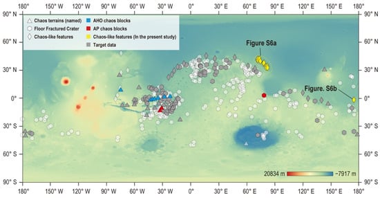
Figure 1.
Global distribution of chaotic terrains named by the International Astronomical Union (IAU; triangles: IAU Planetary Names, cf. https://planetarynames.wr.usgs.gov/ (accessed on 14 January 2020)), floor-fractured craters (FFCs; hexagons: [14]), and chaos-like features (rhombuses: [15]) on Mars, superimposed on an elevation map. Blue and red colors represent chaotic terrains or FFCs that have been investigated previously based on detailed geological analyses (e.g., [1,2,4,5,6,7,16,17]) and which were used as training data for our neural network models in the context of Aromatum-Hydraotes-Oxia-like (or AHO) and Arsinoes-Pyrrhae-like (or AP) chaos blocks, respectively. Yellow circles represent chaos-like features found in the present study (see Figure S6 for the images). Gray color represents the locations of images used as target data.
Previous studies have investigated the formation mechanisms of specific chaos terrains on Mars based on detailed geomorphic and geological analyses (e.g., [1,2,4,5,6,7,13,16,17,18,19]). Some previous studies have suggested that the melting of ground ice or clathrate hydrate and subsequent outbursts of water would have caused surface collapse, based on its association with outflow channels (e.g., [1,2,4,11,13,16,17,20,21]). Depressions of some chaos terrains may have been caused by disruption of the local cryosphere, induced by the intrusion of volcanic sills and the associated heat (Figure 2) [1,2,21]. By contrast, several chaos terrains may have formed through volcano-tectonic activity, such as by the inflation–deflation of magma chambers, without any water activity [5,6,7,12]. Graben, radial and concentric fault systems, orthogonal fractures, lava flows, and pit chains were likely generated through repeated inflation and deflation of magma chambers and a subsequent piecemeal caldera collapse (Figure 3) [5,6,7]. Thanks to high-resolution images taken by recent Mars orbiters (e.g., Mars Reconnaissance Orbiter; MRO), more than 400 chaos-like features have been found (Figure 1; e.g., [14,15,22,23]). Nevertheless, no global-scale classification of Martian chaos and chaos-like features based on their formation mechanisms has been undertaken to date. In addition to chaos and chaos-like features, floor-fractured craters (FFCs) have recently been found on Mars that exhibit fracture features on crater floors that are similar to chaos (e.g., [14,22,23,24]). In general, detailed geological and geomorphic analyses are needed to infer the formation mechanisms of individual chaos terrains. Since such analyses require substantial time investment and knowledge of geology, the number of chaos terrains analyzed is limited despite the rapid increase in the number of identified chaos and chaos-like features and FFCs.
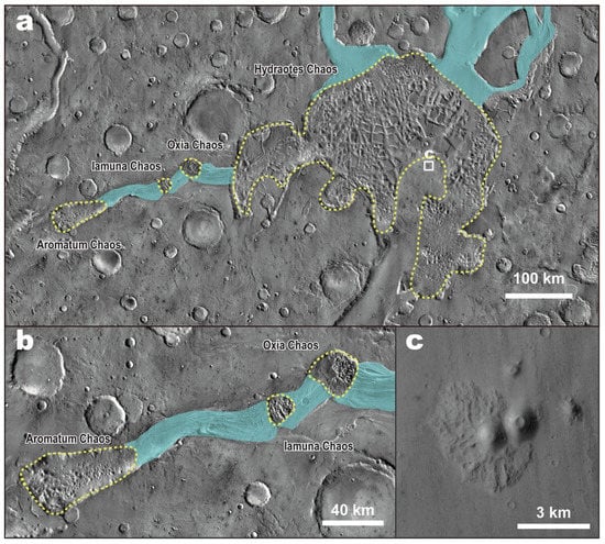
Figure 2.
(a) A THEMIS daytime infrared image of Aromatum Chaos, Hydraotes Chaos, Iamuna Chaos, and Oxia Chaos. The areas surrounded by the yellow dotted line indicate the chaos terrains. The chaos terrains are connected to outflow channels (the area colored light blue). The white box indicates the location of the pitted cones shown in panel (c). (b) A THEMIS daytime infrared image of the Ravi Vallis outflow channel system. The outflow channel system seems to originate from Aromatum Chaos and Iamuna Chaos. (c) A close-up CTX image of a pitted cone near Hydraotes Chaos.
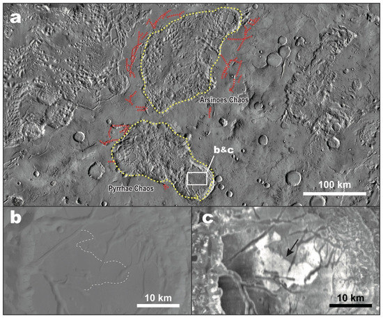
Figure 3.
(a) A THEMIS daytime infrared image of Arsinoes Chaos and Pyrrhae Chaos. The areas surrounded by the yellow dotted lines indicate the chaos terrains. The red dotted lines indicate faults and elongated graben-like depressions possibly formed by volcanic activity [5,6]. The white box indicates the locations of lava flows shown in panels (b,c). (b) A close-up CTX image of lava flows. The white dotted line indicates the outline of lava. (c) A close-up THEMIS thermal inertia image of lava flows. The black arrow indicates the lava flow with high thermal inertia.
Automatic mapping and classification are a new approach in planetary geology (e.g., [25,26,27,28,29]) and can drastically reduce the effort required for investigations of surface features. Nevertheless, to date, there have been a rather limited number of examples of this approach pertaining to geological investigations of Mars (e.g., [28,30,31,32,33,34,35]). Machine learning is increasingly used as an application in industry. It has the potential to reduce the time and effort needed for planetary surface studies when a great quantity of data is available, such as in the case of Mars (e.g., [28,36,37,38]). Such studies using machine learning include automated landform detections on Mars and comparison with Earth’s [25,28]. In addition, the nature of the methodology potentially permits the recognition and characterization of surface features in a manner similar to the approach taken by geologists when performing their surveys. Previous studies applied machine-learning techniques to recognize impact craters on various Solar System bodies (e.g., [39]), as well as dust devil trails on Mars [40]. However, to our knowledge, no previous study has been performed to recognize and classify chaos terrain on Mars using machine learning.
Here, we use imagery machine learning to identify different types of block landforms of chaos terrain with the aim to recognize and classify chaos terrains, chaos-like features, and FFCs, which are distributed globally on Mars. In our machine-learning approach, we used images of block landforms associated with several chaos terrains, whose formation mechanisms were previously investigated, leading to detailed hypotheses based on previous geological and geomorphic analyses. These images were used as training data (see Section 2). We used >1400 images of blocks of chaos and non-chaos features (e.g., impact craters, valley networks, plains) for our training data to develop our neural network models (Section 2). We evaluated the models developed by means of the accuracy, precision, and recall rates obtained for randomly selected test data (Section 3). Then, through the classification of 3148 images of blocks in unclassified chaos terrains, chaos-like features, and FFCs, we obtain and present the global distributions of different types of chaos terrains, plausibly formed through either water or volcano–tectonic activity (Section 4). Finally, based on our results, we discuss the relationship between the distribution of chaos terrain formed through water activity and any hypothesized regions of upwelling groundwater on early Mars (Section 5).
2. Methods
2.1. Outline of the Methodology
We developed fine-tuned convolutional neural network models (so-called ‘classifiers’) that aimed to recognize chaos terrains and non-chaos surface features and classify the recognized chaos terrains into different categories. To this end, we used the architecture of the pre-trained VGG19 model [41], which was originally constructed by the Visual Geometry Group at the University of Oxford (UK). We modified the final layers of the pre-trained VGG19 through fine-tuning for the purpose of classifying chaos terrain on Mars (see Section 2.2 for details of the model).
For the training data, we used three distinct image sources of the Martian surface. These included gray-scale visible geomorphic images taken with the Context Camera (CTX) [42] onboard the MRO at its original resolution of 6 m pixel−1, thermal inertia images taken by the Thermal Emission Imaging System (THEMIS) [43] onboard Mars Odyssey at its original resolution of 100 m pixel−1, and colored elevation images of the Mars digital elevation model (DEM) at its original resolution of 200 m pixel−1, based on data taken by the Mars Orbiter Laser Altimeter (MOLA) [44] on the Mars Global Surveyor and the High-Resolution Stereo Camera (HRSC) [45] on Mars Express. The three types of images were each used as training data for machine learning; that is, we performed training and testing in three ways using the different image sources (see Section 2.3).
To recognize and classify Martian chaos terrain, we defined three categories of surface features. The first encompassed block landforms of chaos that are possibly associated with water activity [1]. We defined this category as chaos terrains directly connected to outflow channels, which are typically found in Aromatum Chaos, Hydraotes Chaos, and Oxia Chaos (Figure 2) [1] (hereafter referred to as Aromatum-Hydraotes-Oxia-like (or AHO) chaos blocks; see Section AHO Chaos Blocks for the details). The second was block landforms of chaos possibly associated with volcanic activity [5,6,7]. We defined the latter category as chaos terrains associated with widespread volcano–tectonic geomorphology (e.g., graben, radial and concentric fault systems, orthogonal fractures, lava flows, and pit chains) and without any outflow channels [5,6,7]. The latter chaos terrains are found in Arsinoes Chaos and Pyrrhae Chaos (Figure 3) (Arsinoes-Pyrrhae-like (or AP) chaos blocks; see Section AP Chaos Blocks for the details). The final type represented Martian surface features other than chaos, including valley networks, impact craters, and plains (‘non-chaos surface features’; see Section Non-Chaos Surface Features). The training data of AHO and AP chaos blocks were images of depressed blocks inside chaos terrains, excluding areas surrounding outflow channels and fault systems that characterized the type of chaos terrain.
Our two categories of AHO and AP chaos blocks might be insufficient to classify all chaos-like features on Mars. In fact, clathrate hydrate destabilization has been suggested as an additional important formation process of chaotic terrain (e.g., [17,20,46]). This may add further complexity to the chaos block landforms. However, to add another classification category, a large number of images representing the new category are required for training. Given the size of chaos blocks (length > several kilometers), widespread chaos terrains (area > 104–105 km2) characterized by well-known formation mechanisms are required for training data. However, the number of such large chaos terrains is limited. In addition, the application of machine learning to the classification of planetary surface images remains challenging. To our knowledge, the present study is the first attempt at applying machine-learning techniques to the classification of chaos terrain. Thus, we opted to use the simplest possible classification categories.
Evaluation of our newly constructed models was performed based on analyses of the transition of the learning curves and a confusion matrix (see Section 2.4). To understand the classification criteria used for our machine-learning approach, we performed data analysis using the Gradient-weighted Class Activation Mapping (Grad-CAM) method [47]. The Grad-CAM method can visualize regions by means of heat maps (Section 2.4.2).
For the target data, we collected images of block landforms of chaos that were provisionally named by the IAU, chaos-like features that are not recognized by the IAU, FFCs, and non-chaos regions (see Section 2.3.2). Since previous work that searched chaos-like features did not cover the Martian surface globally (e.g., [14]), we manually searched for additional chaos-like features on Mars using available CTX and MOLA images to fill gaps in the previous work. We found several chaos-like features on Mars (yellow circles in Figure 1). The target data include chaos-like features that were newly found in the present study.
2.2. Convolutional Neural Network
To develop the classification models, we performed fine-tuning of the final layers of the original VGG19 network [41]. The VGG19 network is a convolutional neural network (CNN), that is, a type of deep neural network [48]. CNNs have been used in many applications, especially for the classification of image data (e.g., [49]). CNNs typically consist of three types of neural network layers (e.g., [50]). The first is a convolutional layer. In CNNs, convolution is carried out through slide filtering, where particular filters (known as kernels) are applied equally to every point in an input image. A convolution layer extracts feature values of an input image using kernels and creates a feature map (e.g., [50]). By adjusting the kernel weight and bias through repeated learning, convolution layers can extract particular features from an input image. A feature map created by a convolution layer is transferred to a pooling layer. Since such a feature map is sensitive to the location of the features in the input image, a pooling layer downsamples the feature map in order to be robust to changes in the feature location in the input image (e.g., [50]). A pooling layer usually performs downsampling by setting a maximum value in a particular region of a feature map as a representative value of that region (max-pooling layer) (e.g., [50]). No weight or bias learning is done in a pooling layer. The final layer is a fully connected layer that summarizes the results from the pooling layer. In addition to these three layers, input and output (softmax) layers were used. The input layer arrayed and contained pixel values for a given image. The output (softmax) layer converted the discrimination result from the neural network into a probability.
In the pre-trained VGG19 network, there are 19 weight layers (16 convolutional and 3 fully connected layers), 5 pooling layers, and a softmax layer (Figure 4a). The pre-trained VGG19 network enables one to improve the accuracy of the deep architecture using a small convolution filter [41]. In this model, an input of an RGB image with a resolution of 224 × 224 pixels2 (i.e., 224 × 224 × 3 matrix) is passed through multiple convolution layers (Figure 4a), which consist of filters with 3 × 3 kernels, as shown in the illustration of Figure 4a. The spatial resolution (width and height) of the input channel is preserved in convolution by the convolution stride as unity (Figure 4a). After multiple convolutions, spatial pooling is performed with 5 max-pooling layers with a 2 × 2 window (Figure 4a). Using the 2 × 2 window, the spatial resolution (width and height) of the input channel is reduced to half in pooling (e.g., 224 × 224 to 112 × 112). The depth of convolution layers (the number of channels) starts with 64 in the first layer and increases by a factor of 2 after the max-pooling layer, reaching up to 512 (Figure 4a). By repeating the convolution and pooling, the pre-trained VGG19 network extracts condensed feature values from a given RGB image. The final max-pooling layer is connected to three fully-connected layers (Figure 4a). The first two fully-connected layers each contain 4096 channels, whereas the last has 1000 channels (Figure 4a). Through the above-mentioned algorithm, the pre-trained VGG19 network yields 1000 class estimated probabilities from an input of a 224 × 224 image (Figure 4a).
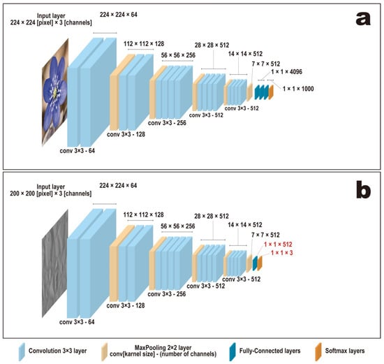
Figure 4.
Architecture of (a) the pre-trained VGG19 network and (b) our revised classifier. There are 19 weight layers (16 convolutional layers and 3 fully connected layers), 5 pooling layers, and 1 softmax layer in the pre-trained VGG19 network. We replaced the fully connected layers and the softmax layer in our classifiers (see the text for details).
Our model was based on the pre-trained VGG19 network. To construct the classifiers for the chaos terrains, we excluded the original final layers of the pre-trained VGG19 network and revised the latter by adding a new final layer that yielded 3-class (i.e., AHO chaos blocks, AP chaos blocks, and non-chaos surface features) estimated probabilities (Figure 4b). We fine-tuned both the final and original VGG19 layers (the first pooling layer) based on the characteristics of our image dataset of the Martian surface (Figure 4b). The other calculation algorithms used in our study were the same as those of the pre-trained VGG19 network shown in Figure 4a.
As for the pre-trained VGG19 network, we included a dropout in our neural network to reduce the overfitting of specific features of the training data during the training [51]. This was done by inactivating some nodes. The probability of inactivating nodes was set at 0.5 based on a previous study [48]. In the calculations, we used data augmentation, where convolutional biases were smoothed out. We also used a cross-entropy loss function in the loss calculations. The initial input images of our study were RGB images with a resolution of 200 × 200 pixel2 (Figure 4b), which is smaller than the RGB images with a resolution of 224 × 224 pixel2 of the pre-trained VGG19 network. Our neural network model performed zero padding to adjust the size of 200 × 200 images to 224 × 224 ones in the first convolution layer (Figure 4b). The typical time required for one cycle of training was about two hours. We repeated the training to find the optimal settings by changing the number of epochs and the batch size. The number of epochs represents the number of times one training dataset was used for repeated learning. When the number of epochs becomes too large, overfitting of specific features in the training data occurs. The number of epochs was set at 15 through trial and error (see Section 3.2).
The batch size is the amount of data in a subset of our training data. Large batch sizes can help reduce the training time [52]; however, a neural network model cannot generalize training data well when the batch size is too large [53]. By contrast, a model with batch sizes that are too small cannot achieve optimal learning [53]. In order to investigate the effect of varying the batch size, we used batch sizes of 32 and 64 in our training. We used neither small batch sizes, such as 8 and 16, nor large ones, such as 128. The former was to avoid trapping in local optima of irregular features of chaotic terrains. The latter was owing to the limited number of the dataset of AP chaos blocks (92 images for the 4 Division and 368 images for 16 Division: see Section 2.3.1 below for details).
2.3. Dataset
2.3.1. Image Data
As described above in Section 2.1, we used the three types, CTX, THEMIS, and MOLA, of images to develop our classifiers. CTX images capture visible geomorphic features on the surface, whereas THEMIS images reflect the thermal inertia of the surface materials. MOLA images are color elevation maps. We will refer to our classifier based on the CTX geomorphic images, the THEMIS thermal inertia images, and the MOLA elevation images as the ‘CTX classifier’, the ‘THEMIS classifier’, and the ‘MOLA classifier’, respectively. CTX geomorphic images reflect differences in surface albedo at visible wavelengths, thus emphasizing the geomorphology of the Martian surface. THEMIS thermal inertia images reflect the roughness and size of regolith on the surface. MOLA elevation images emphasize differences in surface elevations (Figure 5).
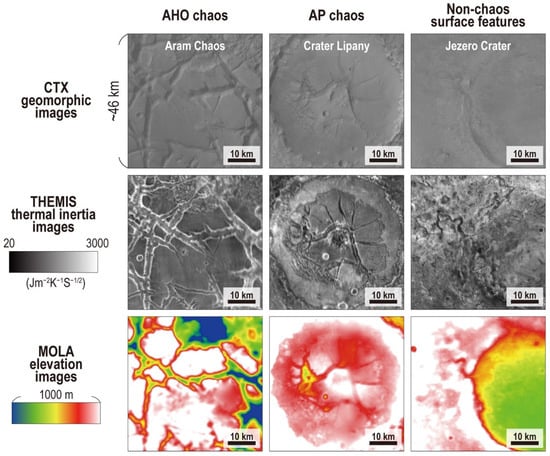
Figure 5.
Comparison of typical CTX geomorphic, THEMIS thermal inertia, and MOLA elevation images for AHO chaos blocks (Aram Chaos), AP chaos blocks (Crater Lipany), and non-chaos surface features (Jezero Crater) used as training data before normalization of pixel values (see the text for details).
The CTX geomorphic and THEMIS thermal inertia mosaic images were collected using Java Mission-planning and Analysis for Remote Sensing (JMARS; https://jmars.asu.edu/ (accessed on 30 October 2020)) [54]. When inputting the image data into the model, we normalized the pixel values of all CTX geomorphic and THEMIS thermal inertia images using histogram equalization, which is an image processing technique to adjust the contrast of images by equalizing the histogram of the number of pixels as a function of pixel value (e.g., [55]). Thus, any difference in the absolute values and dynamic range of the original images obtained in different regions would not affect the model results, but the spatial patterns of the images affect the model results. The incidence angles at which the CTX images were taken are summarized on the JMARS CTX website (http://murray-lab.caltech.edu/CTX/ (accessed on 29 October 2021)). The incidence angles ranged from 30 to 85° but were mostly 40–65°. The MOLA elevation images were collected from the MOLA–HRSC blended digital elevation model using open-source software of the geographic information system, QGIS. To create MOLA elevation images in QGIS, we adopted a color contour chart so that the highest location in an image was colored white and locations 1000 m below the top were colored blue (no images with elevations more than 1000 m in our dataset). We introduced the original images of CTX, THEMIS, and MOLA with different resolutions at the same location to QGIS to convert them to the jpg files with the same resolution of 800 × 800 pixels2. In other words, the image resampling algorithm of QGIS was used to equalize the original difference in resolution.
Preparation of the training images was performed as follows. We first collected 800 × 800 pixels2 images, approximately corresponding to a spatial scale of ~46 × 46 km2 on Mars for the target areas’ latitudes. We then collected mosaic images so as to exclude the surrounding non-chaos surface features from the training data. We chose the locations of the image collection so that we could collect images as much as possible from a chaos terrain. We then divided one original image with a resolution of 800 × 800 pixels2 into four images with a resolution of 400 × 400 pixels2 to increase the number of independent training datasets (hereafter, we will refer to these datasets as the 4 Division data). We also divided the same original image into 16 images with a resolution of 200 × 200 pixels2 (hereafter, we will refer to these datasets as the 16 Division data). To reduce the GPU burden of the calculations, the resolutions of the 4 and 16 Division images were reduced to 200 × 200 and 100 × 100 pixels2, respectively. The number of the 4 Division data is 1/4 times that of the 16 Division data, whereas the resolution of the 4 Division data is twice that of the 16 Division data. By comparing the results of the 4 and 16 Division data, we evaluate the effects of the number of training data and their resolution on the precision of chaos classification.
We prepared a total of 1484 images for the 4 Division training data, including 416 AHO chaos blocks (from 6 locations: see Section AHO Chaos Blocks), 92 AP chaos blocks (from 3 locations: see Section AP Chaos Blocks), and 976 non-chaos surface features (from 126 locations: see Section Non-Chaos Surface Features). For the 16 Division training data, we prepared a total of 5232 images, including 1664 AHO chaos blocks, 368 AP chaos blocks, and 3200 non-chaos surface features. The original 4 Division image data used for the training were the same as for the 16 Division images. The small number of AP chaos block images is because the AP chaos terrains identified by previous work [5,6,7] are limited on Mars.
To train and evaluate our newly developed models, we randomly divided the collected images into two datasets. One is the training data used for training, and the other is the test data that was not used for training. For the training data, we selected 1228 images for 4 Division (and 4400 images for 16 Division) from the collected images. Using the training data, we also obtained the training accuracy, which is the classification accuracy based on the images used in the training. The test data contained 256 and 832 images for 4 and 16 Division, respectively (i.e., 16–17% relative to training data images). The present study did not make the validation data to obtain the validation accuracy because the number of AP chaos block images is limited due to its small areas on Mars. In the present study, the test accuracy was used for the evaluation of model performance. During training, our neural network models produced a training accuracy and a test accuracy after each epoch. Variation curves of the training accuracy and the test accuracy as a function of the number of epochs were obtained using Matplotlib, a Python drawing library.
There is a class imbalance of the image numbers among AHO chaos, AP chaos, and non-chaos surface features in our training data because the number of available images of total AP chaos blocks is only 92 for 4 Division. To evaluate the class imbalance, we prepared the balanced training data by reducing the number of the original images to 92 images each for the 3 categories in addition to the above-mentioned dataset for training and testing.
AHO Chaos Blocks
The image data pertaining to the AHO chaos blocks were images of block landforms inside chaos terrain that were directly connected with outflow channels (e.g., [1,2,4,13,16,21]), although we excluded images of the associated outflow channels from the training and test data. The chaos terrains used for the training data were Aromatum Chaos (1°5′24″S, 317°00′00″E), Hydraotes Chaos (0°48′00″N, 35°24′00″W), Iamuna Chaos (0°16′48″S, 319°23′24″E), Oxia Chaos (0°13′12″N, 320°7′48″E), Hydaspis Chaos (3°12′00″N, 27°6′00″W), Aram Chaos (2°36′00″N, 21°30′00″W), and Echus Chaos (10°69′67″N, 74°81′10″W): e.g., see Figure 1. Since all of these chaotic terrains are associated with outflow channels, they would have formed through outflows of groundwater (e.g., [1,2,4,13,16,21]).
The geological characteristics of the AHO chaos terrains used for the training and test data can be summarized as follows. Aromatum Chaos is directly connected to the Ravi Vallis outflow channel system (Figure 2), strongly suggesting that Aromatum Chaos was the source of outflowing liquid water [1]. The channels may have formed during the Hesperian [1]. The margin of Hydraotes Chaos truncates the Ravi Vallis outflow channel system (Figure 2; [1]), indicating that Hydraotes Chaos postdates the formation of the Ravi Vallis outflow channel system. Iamuna Chaos and Oxia Chaos occur within the Ravi Vallis outflow channels (Figure 2; [1]), which indicates that Iamuna Chaos and Oxia Chaos postdate the formation of the Ravi Vallis outflow channel system. Meresse et al. [2] proposed the dikes/sills emplacement interacting with the cryosphere as a formation mechanism for the overall chaos formation of Hydraotes Chaos. Hydaspis Chaos is suggested to have formed through breakage of extensive subsurface caverns induced by artesian pressurized groundwater (Figure S1; [16]), based on the presence of meandering channels and lobate features. These geological features may have formed through upward emanations of pressurized fluids [16]. The removal of basal materials would have caused subsequent subsidence and fracturing of the cavern’s roof [16]. Based on continuous surface features throughout the Aram Chaos sediments and the surrounding highland terrain, Aram Chaos is considered to have formed through the melting of a buried ice lake (Figure S2; [4,13]).
As described above in Section 2.1, we have randomly chosen the images of chaos blocks for testing and training from the AHO chaos terrains. In addition to this, we have split the dataset for testing and training depending on the region of chaos terrains. This was done because the training and testing using spatially contiguous images of the same terrains could have caused an overestimate of testing accuracy. More specifically, in the split dataset, we have used images of AHO chaos blocks from Aromatum Chaos, Hydaspis Chaos, Iamuna Chaos, and Oxia Chaos as the test dataset, and the images from Hydraotes Chaos, Adam Chaos, and Echus Chaos as the training dataset. We did not split the image dataset of AP chaos blocks because all images of AP chaos were taken from one single region.
AP Chaos Blocks
The training data pertaining to the AP chaos blocks were images of block landforms inside chaos terrain that were associated with widespread volcano–tectonic geomorphology (e.g., graben, radial and concentric fault systems, orthogonal fractures, lava flows, and pit chains) and without any outflow channels [5,6,7,14]. These features suggest that the AP chaos terrains may have been generated through the drainage of magma chambers [5,6,7,14]. The chaos terrains used for the training data were Arsinoes Chaos (8°20′23″S, 332°4′47″E), Pyrrhae Chaos (11°32′23″S, 331°36′00″E), and Crater Lipany (0°13′11″S, 79°40′12″E), see Figure 1.
The geological characteristics of the AP chaos terrains used for the training and test data can be summarized as follows. In Arsinoes Chaos and Pyrrhae Chaos, volcano–tectonic geomorphology (e.g., graben, radial and concentric fault systems, orthogonal fractures, lava flows, and pit chains) are abundant and widespread (Figure 3; [6,7]). On Earth, similar radial and concentric fault systems occur in association with piecemeal caldera collapses [56]. Accordingly, these chaotic terrains are likely to have formed primarily through volcano–tectonic activity, such as by repeated inflation and drainage of magma chambers and subsequent piecemeal caldera collapses [5,6,7]. Crater Lipany is one of the FFCs, with abundant fractures without any outflow channels or flow features (Figure S3; [14]). Pit chains and knobs in the crater have sharp escarpments (Figure S3; [14]), indicative of little erosion through fluvial activity. These observations suggest that the fractures affecting Crater Lipany were likely formed through a volcanic process, such as intrusive volcanism.
Non-Chaos Surface Features
As for our training data pertaining to non-chaos surface features, we chose images of valley networks (260 images), plains with impact craters (196 images), mountains (268 images), trenches (192 images), and streamlined hills (60 images). We collected images of valley networks from the southern highlands, mountains/trenches from the Tharsis region and the Elysium Planitia/mountain, streamlined hills from Chryse Planitia, and plains/impact craters from the southern highlands and the northern lowlands (Figure S4).
2.3.2. Target Data
As for our target data, we chose 125 locations (corresponding to 3148 images for 4 Division data) that exhibit chaos-like features on Mars (Figure 1). They include Galaxias Chaos and Iani Chaos in the circum-Chryse outflow channel region, unnamed chaos terrains, and FFCs. Galaxias Chaos may have formed through subsurface gradual volatile losses due to the capping of the lava unit [57]. The Vastitas Borealis formation is considered to represent H2O-rich residue remaining after huge floods; it is located beneath Galaxias Chaos. The Elysium Rise lava unit overlies Galaxias Chaos. Sublimation of the underlying volatile-rich layer by heat from the lava unit would have induced subsidence [57]. Based on the presence of flood grooves and extensional fractures, Iani Chaos may have formed through extensional fracturing over a pressurized aquifer beneath a thickened cryosphere [11]. We compare our classification with the proposed scenarios [11,57] in Section 4.
2.4. Analytical Methods
2.4.1. Calculations of Accuracy Rates, Precision Rates, Recall Rates, and F-Measures
A confusion matrix shows the relationship between the numbers of true and predicted classifications. We define the terms of Ntrue_x and Nfalse_x as the numbers of true and false classifications, respectively, for type x, where x are AHO chaos blocks (x = AHO), AP chaos blocks (x = AP), or non-chaos surface features (x = nc). For instance, Ntrue_AHO represents the number of images of true AHO chaos blocks that were classified as AHO chaos blocks by our machine-learning algorithm; Nfalse_AHO is the number of images of true AP chaos blocks or non-chaos surface features that were classified as AHO chaos blocks. The relationship between Ntrue_x and Nfalse_x is shown in a confusion matrix (Figure S5).
We used an accuracy rate, A, a precision rate, Px, a recall rate, Rx, and an F-measure, Fx, as our performance measures. An accuracy rate is the most intuitive performance measure and a ratio of correctly predicted classifications to the total classifications. Based on the confusion matrix generated by our model using the tripartite classification, the accuracy rate (A) can be expressed as follows:
The precision rate is the ratio of correctly predicted positive classifications to the total predicted positive classifications. The precision rate is used to evaluate how many images are correctly predicted among actual classifications and can be expressed as follows:
The recall rate is the ratio of correctly predicted positive classifications to all classifications in the actual class. The recall rate is used to evaluate how many images did not overlook among the actual class and is expressed as follows:
where the label in parentheses of term Nfalse_x means the true label of images. For instance, Nfalse_AHO(nc) means the number of images of true non-chaos surface features that are classified as AHO chaos by machine learning. The F-measure is a harmonic mean of the precision rate and recall rate in order to control the precision-recall tradeoff and can be expressed as follows:
We constructed three distinct classifiers for one parameter set (i.e., the batch size and the number of divisions) using different training and testing images, which were randomly chosen each time from the image data. We calculated A, Px, Rx, and Fx three times using three distinct classifiers to obtain the average A, Px, Rx, and Fx values, with their errors (one standard deviation, 1σ), which were used for comparison of our classifiers with the parameter set. Matplotlib software was used to display confusion matrixes.
2.4.2. Heat Map
In general, CNNs are unable to generate classification criteria to reach an assessment because of a failure of the model’s decomposability. To improve the assessment transparency, we used Grad-CAM. Grad-CAM is a method used to define possible criteria for assessment by visualizing the regions [47]. Grad-CAM uses gradients in the final convolutional layer for visualization. Any region that contributes significantly to the output values of a prediction has a large gradient in the final convolutional layer; thus, it is likely to be important for assessment. Grad-CAM can display a heat map of regions, showing large gradients, and, as such, CNN focuses on learning. The Grad-CAM source code was downloaded from the GitHub website (https://github.com/vickyliin/gradcam_plus_plus-pytorch (accessed on 23 October 2020)). The source code was modified in Google Colaboratory to satisfy our calculation setup.
2.5. Search for Chaos-like Features
In addition to reported chaos, chaos-like features, and FFCs, we searched for chaos-like features globally on Mars using available remote sensing images. This was performed by manually viewing many CTX and/or MOLA images with a scale of ~100 km to cover the survey region continuously and globally on Mars. When we found a candidate, we downloaded CTX geomorphic and THEMIS thermal inertia images from JMARS. The survey was performed mainly to map chaos terrains, chaos-like features, and FFCs in the same category and to fill gaps in the global map of FFCs provided by Bamberg et al. [14]. The survey area includes areas in the northern lowlands and southern highlands (Aonia Terra: 60°S97°W; Noachis Terra: 45°S350°E; and Terra Cimmeria: 34.7°S145°E).
By searching for chaos-like features on Mars, we confirmed the conclusions of Bamberg et al. [14] that chaos terrains and chaos-like features are concentrated around the dichotomy boundary and the circum-Chryse outflow channel region. We found new chaos-like features in the Utopia Rupēs and Avernus Colles regions (Figure S6). No new chaos-like features were found in other regions, such as in middle and high latitude regions, the northern lowlands, or the southern highlands (Aonia Terra: 60°S97°W; Noachis Terra: 45°S350°E; and Terra Cimmeria: 34.7°S145°E).
3. Results
3.1. Comparison of Developed Classifiers
Figure 6 shows the results of the test accuracy for the CTX, THEMIS, and MOLA classifiers, adapting for the training data of the 4 Division images and a batch size of 64. Figure 6a–c shows the variation of the test accuracy as a function of the number of learning epochs. The results show that the test accuracy increases with the number of epochs of learning, approaching convergence after 15 epochs.
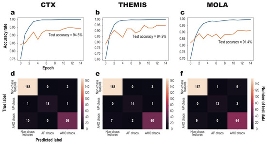
Figure 6.
Typical results of learning curves and confusion matrices for CTX, THEMIS, and MOLA classifiers for 4 Division training data and a batch size of 64. Panels (a–c) are learning curves pertaining to the CTX, THEMIS, and MOLA classifiers, respectively, for 15 epochs of learning. Calculated test and training accuracies are shown as orange and blue lines, respectively. Panels (d–f) are the confusion matrices associated with the CTX, THEMIS, and MOLA classifiers, respectively. Colors and numbers in the confusion matrices represent the test accuracy and the numbers of classified images, respectively, for 15 epochs of learning.
Figure 6a–c also shows the typical variation in the training accuracy. Since the training accuracy is obtained for the example data used for the training, its values should approach ~1.0 (~100% accuracy) over repeated epochs of learning. On the other hand, the test accuracies, obtained by using the dataset that was not used for training, become near constant when epochs of learning become more than 12. Given that fluctuation of the accuracy rate becomes less than 0.03, we use the values of the test accuracy after 15 epochs as representative values for our neural network. The differences between the test and training accuracies are <0.2 after 15 epochs of learning for the 4 Division images and a batch size of 64 (Figure 6). If the difference between the test and training accuracies is large (e.g., >0.2), overfitting of learning may occur in neural network models [58]. Overfitting in machine learning occurs when learning is performed too specifically for given training data and the models cannot generalize the training data adequately. Our results indicate that overfitting would not occur in our neural network model (Figure 6).
Over 15 epochs of learning, the test accuracies of the CTX, THEMIS, and MOLA classifiers reach 94.5%, 94.9%, and 91.4%, respectively (Figure 6). Figure 6d–f shows the typical confusion matrices relating the number of true and predicted classifications for different image categories. As described in Section 2.4.1, we calculated the average values and their errors from the test accuracies of the three distinct classifiers. Table 1 and Table S1 summarize the average test accuracies obtained, the test recall rates, the test precision rates, and the F-measures, as well as their errors, pertaining to our CTX, THEMIS, and MOLA classifiers. The test accuracies, A, for our CTX, THEMIS, and MOLA classifiers (Table 1 and Table S1) are always higher than the random classification accuracy (the probability achieved by randomly assigning a sample to one class) 64–67% for our test data (given 976 images of non-chaos surface features in total 1484 images, the random classification accuracy becomes ~66% for our data). The recall rates, RAP, of AP chaos blocks (the probability of correctly predicting classifications in AP chaos blocks) by the MOLA and THEMIS classifiers are generally low compared with the CTX classifier (Table 1 and Table S1). For instance, the RAP values by the MOLA classifier are ~64–65% for 4 Division and ~40–60% for 16 Division (Table 1 and Table S1). However, the RAP values are much higher than the random classification accuracy of ~6% for AP chaos blocks (given 92 images of AP chaos blocks in total 1484 images, the random classification accuracy for AP chaos blocks becomes ~6%).

Table 1.
Summary of average accuracy rates, precision rates, recall rates, and F-measures with their errors (1σ) for the CTX, THEMIS, and MOLA classifiers. Results for 4 Division images and a batch size of 64. See Supplementary Table S1 for the results for 16 Division images and a batch size of 32 and 64. We adopted the parameter set of Table 1 for application to Martian chaos data.
Comparing the results for different classifiers, the test recall rate, Rnc, of the non-chaos surface features becomes highly independent of the image type (Table 1). This indicates a low probability of overlooking non-chaos surface features. The recall rate, RAHO, of the AHO chaos blocks becomes high for the CTX, THEMIS, and MOLA classifiers (Table 1), whereas the recall rates, RAP, of AP chaos blocks are moderate or relatively low (Table 1). This indicates a possibility that our classifiers, especially the THEMIS and MOLA classifiers, may overlook AP chaos blocks. In addition, Table 1 and Table S1 show that the precision rates, PAP, of AP chaos blocks are generally lower than those of non-chaos surface features, indicating that the probability of false positives is relatively high for AP chaos blocks. The relatively low RAP and PAP rates may be partially due to the small number of both training data and test sets of AP chaos blocks.
Our CTX, THEMIS, and MOLA classifiers can classify non-chaos surface features with high accuracy and low incidence of false positives; however, the MOLA classifier cannot recognize AP chaos blocks well (Table 1). The precision rate, PAP, of AP chaos blocks for the MOLA classifier (~80%) is lower than those for the CTX and THEMIS classifiers (~90%) (Table 1). The high false positive rate (~20%) of AP chaos blocks for the MOLA classifier suggests that it would overlook and classify AHO chaos blocks and non-chaos surface features as AP blocks. On the other hand, the CTX and THEMIS classifiers can recognize AHO and AP chaos blocks with high accuracy (Table 1 and Table S1). The false positive rate of AHO and AP chaos blocks was also low (<10%) (Table 1). Based on these results, we conclude that the CTX and THEMIS classifiers are more appropriate for chaos classification than the MOLA classifier.
3.2. Sensitivity to the Dataset and Batch Size
Figure 6 and Figure S7 show the variations in the test accuracy and confusion matrices for different combinations of batch size (i.e., 32 and 64) and image division (4 Division and 16 Division). Compared with the results shown in Figure 6 and Figure S7, the effects of batch size on the test accuracy seem to be relatively small. In general, fluctuations of test accuracy in a learning curve tend to be large for small batch sizes of the training data due to the results occasionally being trapped in local optima. The latter are generated by noise in the gradient estimates in our machine-learning algorithms [53]. When a batch size is large, noise in gradient estimates tends to be less important, while training with large batch sizes may not allow generalization of the training data (i.e., overfitting). Since Figure 6 and Figure S7 show that overfitting does not occur for batch sizes of 64, we used the classifiers developed with a batch size of 64 for our classification of Martian chaos (Section 4).
Table 1 and Table S1 also compare the average test accuracies of 4 Division and 16 Division images, showing that the test accuracies for 16 Division generally become lower than those for 4 Division. During the training of our classifiers using the 16 Division dataset, the test accuracy fluctuated significantly compared with the 4 Division dataset (Figure S7). This enhanced fluctuation occurred because the small spatial scale of the dataset tends to produce more noise in the gradient estimates in our machine-learning algorithms. 4 Division images have a resolution of 200 × 200 pixels2, corresponding to 23 × 23 km2 on Mars; 16 Division images have a resolution of 100 × 100 pixels2, which corresponds to 11.5 × 11.5 km2 spatially. Since the typical size of blocks of chaos ranges from kilometers to tens of kilometers (e.g., [10]), training based on 16 Division images would not be appropriate to classify block images of chaos. Therefore, we used the classifiers developed using 4 Division images for our classification of Martian chaos (Section 4).
As described in Section 2.3.1 above, the numbers of our training data for the three categories are imbalanced due to the small area of AP chaos terrains. Table S1d shows the test accuracies using the balanced dataset with 92 images for each class. The test accuracies become 87.0%, 81.8%, and 81.3% for the CTX, THEMIS, and MOLA classifiers, respectively, for the balanced dataset. All values became worse than those using the original training data (Table 1) because of the reduction in the size of the dataset. Thus, we used the classifiers developed using the original, imbalanced training dataset for the classification of Martian chaos terrains.
Table 2 shows the results of the precision rate, recall rate, and F-measure for the three classifiers when we have split the training and testing dataset of AHO chaos blocks based on the regions of chaos terrains. Comparing Table 1 and Table 2, the precision rate, recall rate, and F-measure of AHO chaos blocks are unchanged within errors, or even increased, due to the splitting of the dataset (e.g., the precision rate = 0.94 ± 0.02 and 0.92 ± 0.02 for the CTX classifier of the split and original dataset, respectively). This strongly suggests that our model can recognize the AHO chaos blocks regardless of the choice of region for training. However, the precision rate, recall rate, and F-measure of AP chaos blocks are decreased by splitting the AHO dataset based on the region (Table 2) (e.g., the precision rate = 0.60 ± 0.05 and 0.90 ± 0.07 for the CTX classifier of the split and original dataset, respectively). We consider that the decrease in precision for AP chaos blocks occurs because some local, particular features seen in the selected AHO chaos terrains might occur in the AP chaos terrains as well, which may cause misrecognition of some AP chaos blocks. To avoid the artificial error caused by the choice of region, we use the model developed using the randomly chosen dataset for the application to Martian chaos classification in Section 4.
Table 2.
Same as Table 1 but using the split dataset of AHO chaos blocks for testing and training based on the region of the chaos terrains (i.e., the images from Aromatum Chaos, Hydaspis Chaos, Iamuna Chaos, and Oxia Chaos for testing, and the images from Hydraotes Chaos, Adam Chaos, and Echus Chaos for training).
4. Classification of Martian Chaos Terrain
4.1. Distribution of Recognized Chaos on Mars
We applied the CTX, THEMIS, and MOLA classifiers developed using the training data with 4 Division and batch size 64 for recognition and classification of 3148 images of block landforms across chaos terrains, chaos-like features, and FFCs. Although the CTX and THEMIS classifiers would be more appropriate for chaos classification than the MOLA classifier (Section 3.1), the accuracy and recall rate of the MOLA classifier for the training data, including RAP, are higher than the chance level performances (Section 3.1 and Table 1). Thereby, we consider that a comparison of the three classifiers would be valuable to understand the characteristics of each classifier and to categorize the target images of chaos terrains on Mars.
The classification results are summarized in Table 3. For instance, our CTX classifier recognized 1527 images as chaos, including both AHO and AP chaos blocks (Table 3). The relatively high percentage of chaos-like features classified as non-chaos surface features suggests that our three classes may be insufficient to explain all chaos-like features on Mars.
Table 3.
Summary of the numbers of classified images pertaining to the CTX, THEMIS, and MOLA classifiers. The numbers in brackets represent the total numbers of classified images with probabilities of 80% or greater.
Figure 7 shows the spatial distribution of the recognized AHO and AP chaos blocks and of the non-chaos surface features on Mars. Across one terrain, there are multiple images of block landforms that were categorized into different classes. Accordingly, we show pie charts to indicate the percentages of the numbers of the three categories across one terrain in Figure 7. The size of the pie chart represents the number of images. Recognized AHO chaos blocks are distributed around the dichotomy boundary on Mars, whereas recognized AP chaos blocks are mainly located in the circum-Chryse outflow channel region (Figure 7a). The estimated probabilities of recognized chaos being classified as non-chaos surface features are generally low in the circum-Chryse outflow channel region.
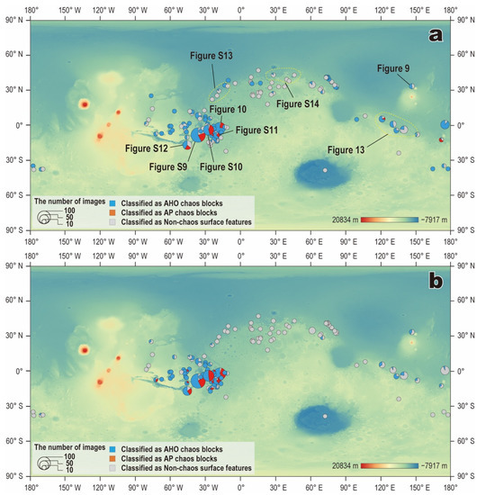
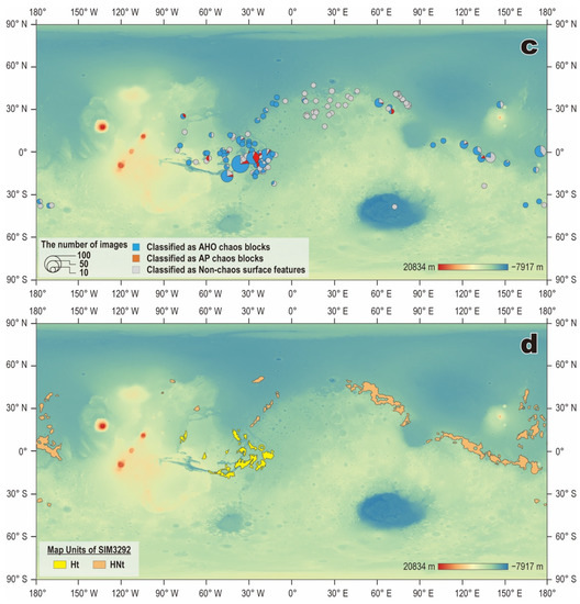
Figure 7.
Global distribution of the classified chaos blocks based on (a) the CTX classifier, (b) the THEMIS classifier, and (c) the MOLA classifier superimposed on a Martian topographic map. The pie charts represent the fractions classified in each category. The sizes of the pie charts represent the number of images at a given location. In panel (a), the locations of the images used in Figures 9, 10, 13, and Figures S9–S14 are shown. Panel (d) shows the global map of chaotic terrain units recognized by geology specialists [24] for comparison. The yellow and orange areas represent the chaotic terrain units on the Hesperian transition unit (Ht) and on the Hesperian and Noachian transition unit (HNt), respectively.
The trends seen for the spatial distributions of the recognized AHO and AP chaos blocks for the CTX classifier are similar to those for the THEMIS and MOLA classifiers (Figure 7b,c). The THEMIS classifier tends to recognize more non-chaos surface features around the dichotomy boundary than the CTX classifier (Figure 7b). The MOLA classifier recognizes more AP chaos blocks around the dichotomy than the other classifiers (Figure 7c). Given the low accuracy of AP chaos block recognition by the MOLA classifier (see Section 3.2) and the fact that both the CTX and THEMIS classifiers do not recognize any AP chaos blocks around the dichotomy boundary (Figure 7), the AP chaos blocks recognized by the MOLA classifier around the dichotomy boundary may include false positives.
Figure 7 shows that around the dichotomy boundary (such as in the Cydonia Mensae region), some AHO chaos blocks recognized by the CTX and MOLA classifiers were recognized by the THEMIS classifier as non-chaos surface features. Some images of newly found chaos-like features (in the present study) are also classified as AHO chaos blocks by the CTX classifier, but they were classified as non-chaos surface features by the THEMIS classifier (Figure 7). Based on Table 1, the precision rates for the recognition of AHO chaos blocks and non-chaos surface features are >85.0% (mostly >90%). Accordingly, the probabilities of returning false positives would be too low to explain the discrepancy in classification results between the CTX/MOLA and THEMIS classifiers.
One possibility that may cause this discrepancy for images from the Cydonia Mensae region is that the surface pattern of chaos terrains in Cydonia Mensae may be overwritten by aeolian landforms with very low thermal inertia. There are multiple intra-crater dune fields in Cydonia Mensae (Figure S8). This region is characterized as an area that tends to accumulate aeolian deposits based on the previously determined global distribution of dune fields and modeled wind directions using Global Climate Models [59]. Figure S8c shows that aeolian landforms (such as wind streaks and drift sands) are frequently found within the chaos terrains of Cydonia Mensae. On the other hand, THEMIS thermal inertia images of the training data pertaining to AHO chaos blocks (i.e., Hydraotes Chaos and Hydaspis Chaos) and recognized AHO chaos blocks (e.g., Aeolis Mensae) do not seem to be covered by aeolian landforms with low thermal inertia (Figure S8e–g). These results suggest that the THEMIS classifier may consider blocks of chaos in Cydonia Mensae as non-chaos surface features because of widespread coverage by aeolian landforms with low thermal inertia.
Figure 8 shows the histograms of AHO chaos blocks, AP chaos blocks, and non-chaos features as functions of latitude, longitude, and elevation. The number and fraction of both AHO and AP chaos blocks become highest in the region of 10°N–10°S in latitude and 0–75°W in longitude. This region corresponds to the circum-Chryse outflow channel region. The AHO chaos blocks tend to be concentrated at relatively low elevations (<−2000 m), which may be consistent with the possible formation scenario of AHO chaos by melting of ground ice and outburst of liquid water.
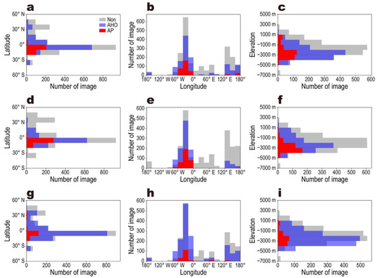
Figure 8.
Histograms of numbers of recognized AHO chaos blocks (blue), AP chaos blocks (red), and non-chaos features (gray) as functions of latitude (a,d,g), longitude (b,e,h), and elevation (c,f,i) on Mars for the different classifiers; CTX (a–c), THEMIS (d–f), and MOLA (g–i).
The spatial distributions of the chaos blocks recognized by our CTX and MOLA classifiers (Figure 7a,c) generally agree with the global map of chaotic terrain units on Mars recognized by geologists [24] (Figure 7d). On the other hand, our THEMIS classifier seems to overlook chaotic terrains in the chaotic terrain units near the dichotomy boundary, including Cydonia Mensae, recognized by geologists [24]. A possible reason that the THEMIS classifier may overlook the chaos terrains around the dichotomy boundary is the occurrence of aeolian landforms, as discussed above. The general agreements of the chaotic blocks recognized by the CTX and MOLA classifiers and the previous chaotic terrain units by Martian geologists [24] support that our classifiers, especially the CTX classifier, have sufficient ability to identify and classify chaotic terrains on Mars.
4.2. Comparison with Previously Proposed Formation Mechanisms
In some chaos terrains where we applied our classifiers, previous studies offered hypotheses of their formation mechanisms based on detailed geological and geomorphic analyses [11,57]. These include Galaxias Chaos and Iani Chaos. In this section, we compare our results with previously proposed formation mechanisms.
Galaxias Chaos, located between the northern Elysium Rise and the eastern Hecates Tholus (34°6′00″N, 213°36′00″W), is suggested to have formed through loss of ground ice due to heat from a capping lava unit [57]. This latter study showed that the elevations of blocks of Galaxias Chaos decreased as a function of increasing distance from Elysium Rise. The Vastitas Borealis Formation (VBF) beneath Galaxia Chaos is considered a residue of water-rich floods based on the similarity in the age of the outflow channels associated with Galaxia Chaos [60]. Given that the Elysium Rise lava unit overlies Galaxias Chaos, sublimation and melting of ice underlying the VBF would have been caused by heat from the lava unit [11,57]. Iani Chaos is also considered to have formed through the melting of subsurface ice. Iani Chaos is located to the southeast of Aram Chaos (3°48′36″S, 342°57′35″E; Figure S10). Based on the presence of flood grooves and extensional fractures, Iani Chaos has also been suggested as having formed through extensional fracturing of the surface due to a pressurized aquifer located beneath a thickened cryosphere [11].
Our CTX, THEMIS, and MOLA classifiers have recognized blocks of chaos in Galaxias Chaos as AHO chaos blocks (Figure 9). Both the CTX and MOLA classifiers recognized large parts of the blocks in Iani Chaos as AHO chaos blocks, combined with small numbers of possible AP chaos blocks (Figure 10). By contrast, the THEMIS classifier recognized them as a mixture of AHO and AP chaos blocks (Figure 10). These comparisons suggest that the results of the classification of chaos in Galaxias and Iani Chaos by our classifiers, especially by the CTX classifier, are generally consistent with the proposed formation mechanisms suggested in previous studies.
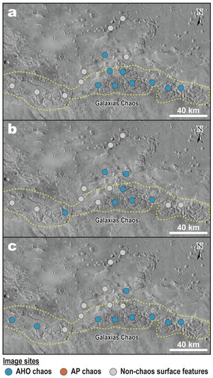
Figure 9.
Classification results of chaos blocks (locations shown by circles) in the Galaxias Chaos region by the (a) CTX, (b) THEMIS, and (c) MOLA classifiers superimposed on a THEMIS daytime infrared image. Circle colors indicate the classification result (blue: AHO chaos blocks; orange: AP chaos blocks; gray: non-chaos surface features). Regions surrounded by yellow dotted lines are chaos-like features.
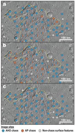
Figure 10.
Classification results of chaos blocks (locations shown by circles) for Iani Chaos: (a) CTX classifier; (b) THEMIS classifier; (c) MOLA classifier. Circle colors indicate the classification result. Circles showing both blue and orange reflect our suggestion that the probabilities of AHO and AP chaos blocks are approximately equal. Regions surrounded by yellow dotted lines are chaos-like features.
4.3. Discussion of Possible Criteria for Classification
Figure 11 shows Grad-CAM heat maps of AHO and AP chaos blocks for our classifiers. Panels (a–c) and (g–i) compare typical images of large blocks (width > 7–8 km) of AHO and AP chaos blocks, respectively; panels (d–f) and (j–l) compare images of small blocks (width < 7–8 km) of AHO and AP chaos blocks, respectively.
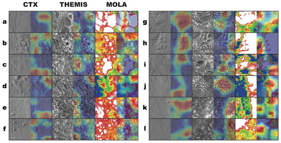
Figure 11.
Grad-CAM heat maps and CTX geomorphic, THEMIS thermal inertia, and MOLA elevation images of blocks classified as (a–f) AHO chaos blocks and (g–l) AP chaos blocks. Panels (a–c) and (g–i) show typical images of large blocks (width > 7–8 km) of AHO and AP chaos blocks, respectively. Panels (d–f) and (j–l) show typical images of small blocks (width < 7–8 km) of AHO and of AP chaos blocks, respectively. Images in panels (a,i,j) were taken from Aureum Chaos, those in (b,f) were taken from Chryse Chaos, and those in (c,e,g,l) were taken from Aurorae Chaos, that in (d) was taken from the western area of chaos near Gale Crater, and those in (h,k) were taken from Eos Chaos.
In the Grad-CAM heat maps, blocks and intervening troughs in both AHO and AP chaos blocks tend to be discerned by the CTX and THEMIS classifiers (Figure 11). In contrast, no particular features seem to be preferred by the MOLA classifier (Figure 11). In the MOLA elevation maps, there is no systematic difference in the elevations of blocks between AHO and AP chaos blocks (Figure 11), which may lead to a lack of detection of blocks and troughs by the MOLA classifier. The fact that no feature seems to be preferred by the MOLA classifier suggests that the categorization by this classifier could be partly affected by large-scale slopes in target regions, seen as a graduation of color in MOLA elevation images. This could cause relatively low accuracies of the MOLA classifier (Table 1).
Comparing the morphology of large blocks in the CTX and THEMIS images, gradients at the edges of AHO chaos blocks tend to be steep (Figure 11a,b), whereas those of AP chaos blocks have gentle slopes (Figure 11g,h). Steep slopes tend to be bright in THEMIS thermal inertia images because of a lack of fine dust on the surface [61]. In addition, troughs between blocks tend to be linear in AHO chaos blocks (Figure 11a,b). The directions of linear troughs of AHO chaos blocks are generally parallel to the directions toward their associated outflow channels (Figure 11a,b). In contrast, troughs of AP chaos blocks are bent according to the blocks’ shapes (Figure 11g–i).
Small blocks of both AHO and AP chaos blocks exhibit crest-topped shapes (Figure 11d–f,j–l). There is often a mesa-like plateau on top of small AP chaos blocks (Figure 11j,k), whereas almost all of the small AHO chaos blocks are crest-topped without plateau tops, even when the block size is similar to that of the AP chaos blocks (Figure 11d–f). In addition, the gradients of the crest-topped AHO chaos blocks are steep, as are those of large AHO chaos blocks (Figure 11a,b).
These differences in the morphology of blocks and troughs between AHO and AP chaos blocks are probably caused by different erosion mechanisms acting on the blocks. Massive outbursts of groundwater would have intensely eroded blocks upon formation of chaos, forming steep slopes at the edges of the blocks and linear troughs. In contrast, surface collapse triggered by draining magma chambers would not have caused any intense erosion by intense fluid outflows. Although we cannot determine the classification criteria adopted by our classifiers solely based on the Grad-CAM heat map, these differences in block morphology might be important for the final classification.
We note that the brightness contrast in the THEMIS images we examined tends to be larger for AHO chaos blocks (Figure 11a,b) compared with that for AP chaos blocks (Figure 11g,h). The THEMIS images of large AHO chaos blocks indicate that parts of the blocks’ top plateaus have lower thermal inertia values than the floors of troughs (Figure 11a,b). On the other hand, thermal inertia values of the top plateaus of AP chaos blocks are similar to those of the floors of troughs (Figure 11g,h). Given that both AHO and AP chaos blocks should have been formed through physically similar processes (i.e., surface collapse), the difference in thermal inertia contrast between these types of chaos blocks could be attributed to material property variations. One possibility is that the materials on the trough floors of AHO chaos blocks may contain smaller amounts of unconsolidated fine sand and dust than those associated with AP chaos blocks, a situation possibly explained by outflows of surface water and/or cementation of dust particles by salts upon evaporation of water. Such a difference inherent in the material properties could also be important for classification, especially for THEMIS classifiers.
5. Implications for Geohydrology and the Cryosphere on Mars
5.1. Types of Chaos Terrain Based on Machine Learning Classification
In our classification, one chaos terrain often contains multiple images of blocks. Through image classification of blocks across a given chaos terrain, we identified two types of chaos terrain on Mars. One is a chaos terrain where both block images classified as AHO and AP chaos blocks co-exist (‘hybrid’ chaos terrain: see Section 5.2 for details). Hybrid chaos terrains are located predominantly around the circum-Chryse outflow channel region (Figure 12), including Aurorae Chaos (Figure S9), Aureum Chaos (Figure S10), Margaritifer Chaos (Figure S11), Iani Chaos (Figure 10), and Eos Chaos (Figure S12). The other type is a chaos terrain where images classified as AHO chaos blocks predominate (‘AHO-dominant’ chaos terrain: see Section 5.3 for details). AHO-dominant chaos terrains are distributed widely around the dichotomy boundary of the northern and southern hemispheres (Figure 7). There are no chaos terrains that are dominated by AP chaos blocks, except for the chaos terrains whose images were used for the training data of AP chaos blocks.
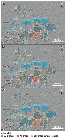
Figure 12.
Classification results of chaos blocks (locations shown by circles) for the circum-Chryse outflow channels chaos region based on the (a) CTX, (b) THEMIS, and (c) MOLA classifiers. Orange and blue shaded areas represent regions whose images were used as training data for the AP and AHO chaos blocks, respectively. Regions within yellow dotted lines represent chaos terrains.
5.2. Hybrid Chaos Terrains
In the circum-Chryse outflow channel region, there are multiple hybrid chaos terrains, i.e., Aurorae Chaos, Aureum Chaos, Margaritifer Chaos, Iani Chaos, and Eos Chaos (Figure 12). All of the CTX, THEMIS, and MOLA classifiers recognized the co-existence of both AHO and AP chaos blocks in these chaos terrains (Figure 12).
Figure 12 shows that blocks classified as AP chaos blocks by the CTX and MOLA classifiers tend to be present near the edges of the chaos terrains adjacent to Arsinoes Chaos and Pyrrhae Chaos (Figure 12; i.e., the southeastern region of Aureum Chaos, the eastern region of Aurorae Chaos, and the western regions of Iani Chaos and Margaritifer Chaos). Arsinoes Chaos and Pyrrhae Chaos were used as training data for the AP chaos blocks (Section AP Chaos Blocks).
Figure 12 also shows that blocks classified as AHO chaos blocks in the hybrid chaos terrains are connected to outflow channels. The outflow channels associated with the hybrid chaos terrains are located north of the chaos terrains, away from the regions of AP chaos blocks (Figure 12). These outflow channels are connected to chaos terrains (Aram Chaos, Hydaspis Chaos, Hydraotes Chaos) that were used as training data for AHO chaos blocks (Figure 11). The outflow channels are also connected to AHO-dominant chaos terrains (Chryse Chaos) classified by the present study (Figure 12). These results suggest that outbursts of groundwater that formed the outflow channels have supplied large volumes of water to the downstream regions of these AHO-dominant chaos terrains.
There are a few possible interpretations of the hybrid chaos terrains in the circum-Chryse outflow channel region. One is that our three categories (i.e., AHO chaos blocks, AP chaos blocks, and non-chaos surface features) are insufficient to classify all chaos-like terrains on Mars. If the chaos terrains in the circum-Chryse outflow channel region were formed via geological processes other than those formed AHO-type chaos and AP-type chaos, the chaos-like terrains might not be well classified in one category.
Another possible interpretation is that the terrains were indeed formed by a combination of volcano–tectonic activities (AP chaos terrains) (e.g., [5,6,7,14]) and outflowing of groundwater (AHO chaos terrains) (e.g., [1,2,4,13,16,21]). If inflation of magma chambers through upwelling of magma occurred in the region [62], the upwelling of magma also increased the geothermal heat flux around this area. In regions where ground ice was present, the increased subsurface temperatures could have melted ground ice, resulting in outbursts of groundwater and the subsequent formation of catastrophic outflow channels (e.g., [1,2]). The source of ground ice may have been fluvial and glacial sediments deposited into a clastic wedge in the southern circum-Chryse region [63]. To conclude this scenario, more detailed geomorphic observations would be required.
5.3. AHO-Dominant Chaos Terrains
Our results show that AHO-dominant chaos terrains are present around highly brecciated, fretted areas in Aeolis Mensae, Nepenthes Mensae, and Cydonia Mensae around the dichotomy boundary (Figure 7; see Figure 13 for Aeolis Mensae and Nepenthes Mensae; see Figure S13 for Cydonia Mensae). Previous work has proposed that the fretted areas would have formed in response to glacial erosion in the early Hesperian [64]. On Earth, many valleys in fretted terrains exhibit characteristics of glacial troughs (i.e., U-shaped valleys), which also occur on these mensae on Mars [64]. However, previous work has suggested that the chaos terrains near these mensae would have formed through surface collapses owing to the removal of subsurface volatiles, as there are no outflow channels associated with the chaos terrains (e.g., [16]). However, valleys are observed near the fretted terrains of Cydonia Mensae. Fretted terrains in Aeolis Mensae may be composed of friable sediments [65], which are interpreted as landforms that were attributed to ice and/or water activity. In addition to these previous studies, we find that the edges of chaos blocks in these fretted areas tend to be smooth (Figure S14), and crest-topped blocks are present in chaos terrains in these areas (Figure S14). These geomorphic features suggest that the surface/ground ice would once have been abundant in these areas and may have been a source of volatiles for AHO chaos terrains if AHO chaos terrains were formed by groundwater activities.
In contrast to Cydonia Mensae, Aeolis Mensae, and Nepenthes Mensae, we found few water-related chaos block terrains associated with Deuteronilus Mensae and Protonilus Mensae around the dichotomy boundary (Figure S15), except for a few images of Deuteronilus Mensae. Since most images from these regions are classified as non-chaos surface features regardless of the classifier used, we consider that chaos-like features in these regions might have been formed by mechanisms other than outbursts of ground water or volcanic activity.
The regions of AHO-dominant chaos terrain (i.e., Cydonia Mensae, Nepenthes Mensae, and Aeolis Mensae: Figure 7) seem to correlate well with the suggested regions of upwelling groundwater on Hesperian Mars [66]. It is suggested that the main stage of the hydrological cycles on Mars shifted from the near-surface to the subsurface around the Hesperian (e.g., [67]). Groundwater upwelling would have occurred at the dichotomy boundary between the southern highlands and the northern lowlands on Hesperian Mars [66]. Since the rise of Tharsis should have caused the uplift of the antipodal Arabia bulge (Figure 14), the regions between Tharsis and the Arabia bulge became topographic lows [68]. This includes the regions near Nepenthes Mensae, Aeolis Mensae, and Cydonia Mensae (Figure 14). Then, groundwater flows would have been concentrated in these topographic lows at the dichotomy boundary, resulting in a shallow groundwater table (Figure 14; [66]).
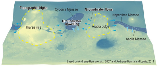
Figure 14.
Schematic illustration of global groundwater flows on Hesperian Mars, based on Andrews–Hanna et al. [66,71]. Groundwater is considered to have flowed from the southern highlands to the northern lowlands (cyan bold arrows). Groundwater would have upwelled at local steep slopes and impact craters at the dichotomy boundary. Owing to the rise of Tharsis and the antipodal topographic highs of the Arabia bulge (yellow dashed lines), groundwater flows would have been concentrated around the regions (Aeolis Mensae, Cydonia Mensae, and Nepenthes Mensae) between them (blue arrows). Blueish hatched areas represent regions where groundwater could have been concentrated.
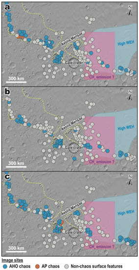
Figure 13.
Classification results of chaos blocks (locations shown by circles) for the Aeolis Mensae and Nepenthes Mensae regions based on the (a) CTX, (b) THEMIS, and (c) MOLA classifiers. Regions surrounded by yellow dotted lines are chaos-like features. Blue and pink areas, respectively, represent the Medusae Fossae Formation (MFF), with high water equivalent height (WEH) contents [69], and regions that are likely sources of a CH4 spike found in the Gale Crater, as suggested by the Global Circulation Model [70]. The black dotted circle represents the Gale Crater.
6. Conclusions
Knowledge of the global distribution and activity of groundwater/ground ice is critical to understanding the evolution of hydrology, habitability, and in situ water resource use for future crewed missions to Mars. In the present study, we performed machine learning for the recognition and classification of Martian chaos terrain based on previously proposed formation mechanisms. To this end, we developed three distinct classifiers (CTX, THEMIS, and MOLA) using different sources of remote-sensing data. We consider that the CTX classifier is the most reliable for classifying chaos-like features. This is because both the CTX and THEMIS classifiers showed high accuracy rates in recognizing chaos, but the results of the THEMIS classifier tend to be influenced by recent surface coverage of dust or volcanic ash. We applied our newly developed classifiers to block landforms appearing in images of chaos terrains, chaos-like features, and FFCs on Mars. We obtained the global distribution of images of chaos blocks presumably formed by water activity (AHO chaos blocks) and volcano–tectonic activity (AP chaos blocks) on Mars.
Automated classification of geological features using machine learning remains challenging for remote-sensing data for planetary bodies. The major assumption in our study is that the origins of the chaos terrains used as training data are well-understood and reliable for our purpose. Therefore, the interpretations derived from our application depend heavily on this assumption. In addition, our three classes may be too few to explain all the chaos-like features on Mars. Despite these uncertainties, the results of the present study can be summarized as follows.
- Our new classifiers achieve high accuracy rates in recognizing chaos on Mars. The accuracies achieved are 93.5% ± 0.7%, 91.3% ± 2.6%, and 88.5% ± 2.1% for the CTX, THEMIS, and MOLA classifiers, respectively, with 4 Division images and a batch size of 64 (Table 1).
- The chaos terrains recognized by our classifiers are predominantly distributed in the circum-Chryse outflow channel region and near the dichotomy boundary (Figure 7). We identified two types of chaos terrain on Mars. One is hybrid chaos terrain, where images classified as both AHO and AP chaos blocks co-exist in one terrain. The other is AHO-dominant chaos terrain, where AHO chaos blocks are predominant. Hybrid chaos terrains are located predominantly around the circum-Chryse outflow channel region, whereas AHO-dominant chaos terrains are distributed widely around the dichotomy boundary.
- We suggest that AHO chaos blocks tend to be more eroded than AP chaos blocks, possibly due to outbursts of groundwater flows. The detailed differences in morphology of the blocks and troughs may be important for the final classification.
- Hybrid chaos terrains in the circum-Chryse outflow channels region could have been formed by a combination of uplift and infiltration of magma chambers and subsequent melting ground ice, although more detailed geomorphic observations are necessary to conclude this hypothesis.
- The regions of AHO-dominant chaos terrains near Cydonia Mensae, Nepenthes Mensae, and Aeolis Mensae correlate with the suggested regions of upwelling groundwater on Hesperian Mars [66]. This further implies that the water source that formed the AHO-dominant chaos terrains at the dichotomy boundary might be remnant frozen groundwater.
Supplementary Materials
The following supporting information can be downloaded at: https://www.mdpi.com/article/10.3390/rs14163883/s1. Supplementary Figures contain data regarding images of terrains we have used as training data, results of learning curves and confusion matrices for other training settings (Division = 4 or 16, BS = 32 or 64), and classification results of chaos blocks in other chaotic terrains. Supplementary Table contains data regarding evaluation summary for other training settings (Division = 4 or 16, BS = 32 or 64).
Author Contributions
Conceptualization, Y.S.; methodology, H.S. and N.G.; software, H.S. and N.G.; validation, H.S.; formal analysis, H.S. and N.G.; investigation, H.S.; resources, Y.S.; data curation, H.S.; writing—original draft preparation, H.S. and Y.S.; writing—review and editing, N.G. and G.K.; visualization, H.S.; supervision, Y.S.; funding acquisition, Y.S. All authors have read and agreed to the published version of the manuscript.
Funding
This study was supported by Grants-in-Aid for Scientific Research (KAKENHI JSPS Grants JP17H06456, JP20H00195, and JP21H04515).
Data Availability Statement
All original image datasets and our newly developed classifiers are available for download from an open access repository (Shozaki et al. [72]).
Acknowledgments
This study was supported by Grants-in-Aid for Scientific Research (KAKENHI JSPS Grants JP17H06456, JP20H00195, and JP21H04515). We are grateful to the editors Kirby Runyon, Angela M. Dapremont, and Alexandra Matiella-Novak. We are also grateful to three anonymous reviewers for their constructive comments.
Conflicts of Interest
The authors declare no conflict of interest.
References
- Leask, H.J.; Wilson, L.; Mitchell, K.L. Formation of Aromatum Chaos, Mars: Morphological Development as a Result of Volcano-Ice Interactions. J. Geophys. Res. E Planets 2006, 111, E08071. [Google Scholar] [CrossRef] [Green Version]
- Meresse, S.; Costard, F.; Mangold, N.; Masson, P.; Neukum, G. Formation and Evolution of the Chaotic Terrains by Subsidence and Magmatism: Hydraotes Chaos, Mars. Icarus 2008, 194, 487–500. [Google Scholar] [CrossRef]
- Collins, G.; Nimmo, F. Chaotic Terrain on Europa. In Europa; University of Arizona Press: Tucson, AZ, USA, 2009; pp. 259–281. [Google Scholar]
- Roda, M.; Kleinhans, M.G.; Zegers, T.E.; Oosthoek, J.H.P. Catastrophic Ice Lake Collapse in Aram Chaos, Mars. Icarus 2014, 236, 104–121. [Google Scholar] [CrossRef] [Green Version]
- Luzzi, E.; Rossi, A.P.; Pozzobon, R. Confined Channels and Collapse Features in Arsinoes and Pyrrhae Chaos (Mars): Hints for a Volcano-Tectonic Origin. In Proceedings of the 21st European Geosciences Union General Assembly, Vienna, Austria, 7–12 April 2019. [Google Scholar]
- Luzzi, E.; Rossi, A.P.; Carli, C.; Altieri, F. Tectono-Magmatic, Sedimentary, and Hydrothermal History of Arsinoes and Pyrrhae Chaos, Mars. J. Geophys. Res. Planets 2020, 125, e2019JE006341. [Google Scholar] [CrossRef]
- Luzzi, E.; Rossi, A.P.; Massironi, M.; Pozzobon, R.; Corti, G.; Maestrelli, D. Caldera Collapse as the Trigger of Chaos and Fractured Craters on the Moon and Mars. Geophys. Res. Lett. 2021, 48, e2021GL092436. [Google Scholar] [CrossRef]
- Skjetne, H.L.; Singer, K.N.; Hynek, B.M.; Knight, K.I.; Schenk, P.M.; Olkin, C.B.; White, O.L.; Bertrand, T.; Runyon, K.D.; McKinnon, W.B.; et al. Morphological Comparison of Blocks in Chaos Terrains on Pluto, Europa, and Mars. Icarus 2021, 356, 113866. [Google Scholar] [CrossRef]
- Rodriguez, J.A.P.; Leonard, G.J.; Kargel, J.S.; Domingue, D.; Berman, D.C.; Banks, M.; Zarroca, M.; Linares, R.; Marchi, S.; Baker, V.R.; et al. The Chaotic Terrains of Mercury Reveal a History of Planetary Volatile Retention and Loss in the Innermost Solar System. Sci. Rep. 2020, 10, 4737. [Google Scholar] [CrossRef] [Green Version]
- Pedersen, G.B.M. Chaotic Terrain (Mars). In Encyclopedia of Planetary Landforms; Springer: New York, NY, USA, 2014; pp. 1–6. ISBN 9781461492139. [Google Scholar]
- Warner, N.H.; Gupta, S.; Kim, J.R.; Muller, J.P.; Le Corre, L.; Morley, J.; Lin, S.Y.; McGonigle, C. Constraints on the Origin and Evolution of Iani Chaos, Mars. J. Geophys. Res. E Planets 2011, 116, E06003. [Google Scholar] [CrossRef] [Green Version]
- Sharp, R.P. Mars: Fretted and Chaotic Terrains. J. Geophys. Res. 1973, 78, 4073–4083. [Google Scholar] [CrossRef] [Green Version]
- Zegers, T.E.; Oosthoek, J.H.P.; Rossi, A.P.; Blom, J.K.; Schumacher, S. Melt and Collapse of Buried Water Ice: An Alternative Hypothesis for the Formation of Chaotic Terrains on Mars. Earth Planet. Sci. Lett. 2010, 297, 496–504. [Google Scholar] [CrossRef]
- Bamberg, M.; Jaumann, R.; Asche, H.; Kneissl, T.; Michael, G.G. Floor-Fractured Craters on Mars—Observations and Origin. Planet. Space Sci. 2014, 98, 146–162. [Google Scholar] [CrossRef]
- Rossi, A.P.; Huvenne, V.A.; Henriet, J.P.; Wagner, R.; Hauber, E.; Chicarro, A.; Di Lorenzo, S.; Neukum, G.; HRSC Co-Investigator Team. A Buried Earth Analogue to Martian Chaotic Terrains. In Proceedings of the 37th Annual Lunar and Planetary Science Conference, League City, TX, USA, 13–17 March 2006; p. 1573. [Google Scholar]
- Rodriguez, J.A.P.; Sasaki, S.; Kuzmin, R.O.; Dohm, J.M.; Tanaka, K.L.; Miyamoto, H.; Kurita, K.; Komatsu, G.; Fairén, A.G.; Ferris, J.C. Outflow Channel Sources, Reactivation, and Chaos Formation, Xanthe Terra, Mars. Icarus 2005, 175, 36–57. [Google Scholar] [CrossRef]
- Rodriguez, J.A.P.; Kargel, J.; Crown, D.A.; Bleamaster, L.F.; Tanaka, K.L.; Baker, V.; Miyamoto, H.; Dohm, J.M.; Sasaki, S.; Komatsu, G. Headward Growth of Chasmata by Volatile Outbursts, Collapse, and Drainage: Evidence from Ganges Chaos, Mars. Geophys. Res. Lett. 2006, 33, 2–6. [Google Scholar] [CrossRef]
- Kargel, J.S.; Furfaro, R.; Prieto-Ballesteros, O.; Rodriguez, J.A.P.; Montgomery, D.R.; Gillespie, A.R.; Marion, G.M.; Wood, S.E. Martian Hydrogeology Sustained by Thermally Insulating Gas and Salt Hydrates. Geology 2007, 35, 975–978. [Google Scholar] [CrossRef]
- Chapman, M.G.; Tanaka, K.L. Related Magma-Ice Interactions: Possible Origins of Chasmata, Chaos, and Surface Materials in Xanthe, Margaritifer, Meridiani Terrae, Mars. Icarus 2002, 155, 324–339. [Google Scholar] [CrossRef] [Green Version]
- Komatsu, G.; Kargel, J.S.; Baker, V.R.; Strom, R.G.; Ori, G.G.; Mosangini, C.; Tanaka, K.L. A Chaotic Terrain Formation Hypothesis: Explosive Outgas and Outlow by Dissociation of Clathrate on Mars. In Proceedings of the 31st Annual Lunar and Planetary Science Conference, Houston, TX, USA, 13–17 March 2000. [Google Scholar]
- Coleman, N.M. Martian Megaflood-Triggered Chaos Formation, Revealing Groundwater Depth, Cryosphere Thickness, and Crustal Heat Flux. J. Geophys. Res. 2005, 110, E12S20. [Google Scholar] [CrossRef] [Green Version]
- Korteniemi, J.; Aittola, M.; Lahtela, H.; Öhman, T.; Raitala, J. Martian Floor-Fractured Craters vs. Craters with Irregular Depressions. In Proceedings of the 37th Annual Lunar and Planetary Science Conference, League City, TX, USA, 13–17 March 2006; p. 2145. [Google Scholar]
- Korteniemi, J.; Aittola, M.; Öhman, T.; Raitala, J. Floor-Fractured Craters on the Terrestrial Planets—The Martian Perspective. In Proceedings of the 40th ESLAB Symposium—First International Conference on Impact Cratering in the Solar System, Noordwijk, The Netherlands, 8–12 May 2006; pp. 193–198. [Google Scholar]
- Tanaka, K.L.; Skinner, J.A.; Dohm, J.M.; Irwin, R.P.; Kolb, E.J.; Fortezzo, C.M.; Platz, T.; Michael, G.G.; Hare, T.M. Geologic Map of Mars: U.S. Geological Survey Scientific Investigations Map 3292; United States Geological Survey: Reston, VA, USA, 2014. [CrossRef]
- Stepinski, T.F.; Ghosh, S.; Vilalta, R. Automatic Recognition of Landforms on Mars Using Terrain Segmentation and Classification. In Proceedings of the International Conference on Discovery Science, Barcelona, Spain, 7–10 October 2006; pp. 255–266. [Google Scholar]
- Yamamoto, S.; Matsunaga, T.; Nakamura, R.; Sekine, Y.; Hirata, N.; Yamaguchi, Y. Rotational Pixel Swapping Method for Detection of Circular Features in Binary Images. IEEE Trans. Geosci. Remote Sens. 2015, 53, 710–723. [Google Scholar] [CrossRef]
- Vamshi, G.T.; Martha, T.R.; Vinod Kumar, K. An Object-Based Classification Method for Automatic Detection of Lunar Impact Craters from Topographic Data. Adv. Sp. Res. 2016, 57, 1978–1988. [Google Scholar] [CrossRef]
- Palafox, L.F.; Hamilton, C.W.; Scheidt, S.P.; Alvarez, A.M. Automated Detection of Geological Landforms on Mars Using Convolutional Neural Networks. Comput. Geosci. 2017, 101, 48–56. [Google Scholar] [CrossRef]
- Cambioni, S.; Bennett, C.A.; Walsh, K.J.; DellaGiustina, D.N.; Golish, D.R.; Becker, K.J.; Lauretta, D.S. A Search for Smooth Terrains on Asteroid (101955) Bennu Using Machine Learning. In Proceedings of the EPSC-DPS Joint Meeting 2019, Geneva, Switzerland, 15–20 September 2019; p. EPSC-DPS2019. [Google Scholar]
- Komatsu, G.; Ori, G.G.; Cardinale, M.; Dohm, J.M.; Baker, V.R.; Vaz, D.A.; Ishimaru, R.; Namiki, N.; Matsui, T. Roles of Methane and Carbon Dioxide in Geological Processes on Mars. Planet. Space Sci. 2011, 59, 169–181. [Google Scholar] [CrossRef]
- Wilhelm, T.; Geis, M.; Püttschneider, J.; Sievernich, T.; Weber, T.; Wohlfarth, K.; Wöhler, C. DoMars16k: A Diverse Dataset for Weakly Supervised Geomorphologic Analysis on Mars. Remote Sens. 2020, 12, 3981. [Google Scholar] [CrossRef]
- Pardo-Igúzquiza, E.; Dowd, P.A.; Naor, R. Automatic Mapping and Spatial Analysis of High Spatial Resolution Closed Terrain Depressions and Mounds on Martian Landscapes. Icarus 2021, 369, 114632. [Google Scholar] [CrossRef]
- Nodjoumi, G.; Pozzobon, R.; Rossi, A.P. Deep Learning Object Detection for Mapping Cave Candidates on Mars: Building up the Mars Global Cave Candidate Catalog (MGC3). In Proceedings of the 52th Lunar and Planetary Science Conference, The Woodlands, TX, USA, 15–19 March 2021; p. 1316. [Google Scholar]
- Rubanenko, L.; Perez-Lopez, S.; Schull, J.; Lapotre, M.G.A. Automatic Detection and Segmentation of Barchan Dunes on Mars and Earth Using a Convolutional Neural Network. IEEE J. Sel. Top. Appl. Earth Obs. Remote Sens. 2021, 14, 9364–9371. [Google Scholar] [CrossRef]
- Rajaneesh, A.; Vishnu, C.L.; Oommen, T.; Rajesh, V.J.; Sajinkumar, K.S. Machine Learning as a Tool to Classify Extra-Terrestrial Landslides: A Dossier from Valles Marineris, Mars. Icarus 2022, 376, 114886. [Google Scholar] [CrossRef]
- Wagstaff, K.; Lu, S.; Dunkel, E.; Grimes, K.; Zhao, B.; Cai, J.; Cole, S.B.; Doran, G.; Francis, R.; Lee, J.; et al. Mars Image Content Classification: Three Years of Nasa Deployment and Recent Advances. In Proceedings of the AAAI Conference on Artificial Intelligence, Online, 2–9 February 2021; Volume 35, pp. 15204–15213. [Google Scholar]
- Nagle-McNaughton, T.P.; Scuderi, L.A.; Erickson, N. Squeezing Data from a Rock: Machine Learning for Martian Science. Geosciences 2022, 12, 248. [Google Scholar] [CrossRef]
- Plebani, E.; Ehlmann, B.L.; Leask, E.K.; Fox, V.K.; Dundar, M.M. A Machine Learning Toolkit for CRISM Image Analysis. Icarus 2022, 376, 114849. [Google Scholar] [CrossRef]
- Silburt, A.; Ali-Dib, M.; Zhu, C.; Jackson, A.; Valencia, D.; Kissin, Y.; Tamayo, D.; Menou, K. Lunar Crater Identification via Deep Learning. Icarus 2019, 317, 27–38. [Google Scholar] [CrossRef] [Green Version]
- Gichu, R.; Ogohara, K. Segmentation of Dust Storm Areas on Mars Images Using Principal Component Analysis and Neural Network. Prog. Earth Planet. Sci. 2019, 6, 19. [Google Scholar] [CrossRef]
- Simonyan, K.; Zisserman, A. Very Deep Convolutional Networks for Large-Scale Image Recognition. arXiv 2014, arXiv:1409.1556. [Google Scholar]
- Malin, M.C.; Bell, J.F.; Cantor, B.A.; Caplinger, M.A.; Calvin, W.M.; Clancy, R.T.; Edgett, K.S.; Edwards, L.; Haberle, R.M.; James, P.B.; et al. Context Camera Investigation on Board the Mars Reconnaissance Orbiter. J. Geophys. Res. E Planets 2007, 112, E05S04. [Google Scholar] [CrossRef] [Green Version]
- Christensen, P.R.; Jakosky, B.M.; Kieffer, H.H.; Malin, M.C.; McSween, H.Y., Jr.; Nealson, K.; Mehall, G.; Silverman, S.; Ferry, S. The Thermal Emission Imaging System (THEMIS) Instrument for the Mars 2001 Orbiter. In Proceedings of the Workshop on Mars 2001: Integrated Science in Preparation for Sample Return and Human Exploration, Houston, TX, USA, 2–4 October 1999; p. 28. [Google Scholar]
- Zuber, M.T.; Smith, D.E.; Solomon, S.C.; Muhleman, D.O.; Head, J.W.; Garvin, J.B.; Abshire, J.B.; Bufton, J.L. The Mars Observer Laser Altimeter Investigation. J. Geophys. Res. Planets 1992, 97, 7781–7797. [Google Scholar] [CrossRef]
- Neukum, G.; Jaumann, R. HRSC: The High Resolution Stereo Camera of Mars Express. In Mars Express: The Scientific Payload; European Space Agency: Paris, France, 2004; Volume 1240, pp. 17–35. [Google Scholar]
- Rodríguez, J.A.P.; Kargel, J.S.; Tanaka, K.L.; Crown, D.A.; Berman, D.C.; Fairén, A.G.; Baker, V.R.; Furfaro, R.; Candelaria, P.; Sasaki, S. Secondary Chaotic Terrain Formation in the Higher Outflow Channels of Southern Circum-Chryse, Mars. Icarus 2011, 213, 150–194. [Google Scholar] [CrossRef]
- Selvaraju, R.R.; Cogswell, M.; Das, A.; Vedantam, R.; Parikh, D.; Batra, D. Grad-CAM: Visual Explanations from Deep Networks via Gradient-Based Localization. Int. J. Comput. Vis. 2020, 128, 336–359. [Google Scholar] [CrossRef] [Green Version]
- Deng, J.; Dong, W.; Socher, R.; Li, L.-J.; Li, K.; Li, F.-F. ImageNet: A Large-Scale Hierarchical Image Database. In Proceedings of the 2009 IEEE Conference on Computer Vision and Pattern Recognition, Miami, FL, USA, 20–25 June 2009; pp. 248–255. [Google Scholar]
- O’Shea, K.; Nash, R. An Introduction to Convolutional Neural Networks. arXiv 2015, arXiv:1511.08458. [Google Scholar]
- Bishop, C.M. Pattern Recognition and Machine Learning; Springer: New York, NY, USA, 2006; ISBN 978-1-4939-3843-8. [Google Scholar]
- Srivastava, N.; Hinton, G.; Krizhevsky, A.; Sutskever, I.; Salakhutdinov, R. Dropout: A Simple Way to Prevent Neural Networks from Overfitting. J. Mach. Learn. Res. 2014, 15, 1929–1958. [Google Scholar]
- Smith, S.L.; Kindermans, P.-J.; Ying, C.; Le, Q.V. Don’t Decay the Learning Rate, Increase the Batch Size. In Proceedings of the 6th International Conference on Learning Representations (ICLR), Vancouver, BC, Canada, 30 April–3 May 2018. [Google Scholar]
- Keskar, N.S.; Mudigere, D.; Nocedal, J.; Smelyanskiy, M.; Tang, P.T.P. On Large-Batch Training for Deep Learning: Generalization Gap and Sharp Minima. In Proceedings of the 5th International Conference on Learning Representations (ICLR), Toulon, France, 24–26 April 2017. [Google Scholar]
- Christensen, P.R.; Engle, E.; Anwar, S.; Dickenshied, S.; Noss, D.; Gorelick, N.; Weiss-Malik, M. JMARS-a Planetary GIS. In Proceedings of the AGU Fall Meeting, San Francisco, CA, USA, 13–18 December 2009; p. IN22A-06. [Google Scholar]
- Hummel, R.A. Image Enhancement by Histogram Transformation. Comput. Graph. Image Process. 1977, 6, 184–185. [Google Scholar] [CrossRef]
- Troll, V.R.; Walter, T.R.; Schmincke, H.-U. Cyclic Caldera Collapse: Piston or Piecemeal Subsidence? Field and Experimental Evidence. Geology 2002, 30, 135. [Google Scholar] [CrossRef]
- Pedersen, G.B.M.; Head, J.W. Chaos Formation by Sublimation of Volatile-Rich Substrate: Evidence from Galaxias Chaos, Mars. Icarus 2011, 211, 316–329. [Google Scholar] [CrossRef]
- Cogswell, M.; Ahmed, F.; Girshick, R.; Zitnick, L.; Batra, D. Reducing Overfitting in Deep Networks by Decorrelating Representations. In Proceedings of the 4th International Conference on Learning Representations (ICLR), San Juan, Puerto Rico, 2–4 May 2016. [Google Scholar]
- Hayward, R.K.; Titus, T.N.; Michaels, T.I.; Fenton, L.K.; Colaprete, A.; Christensen, P.R. Aeolian Dunes as Ground Truth for Atmospheric Modeling on Mars. J. Geophys. Res. E Planets 2009, 114, E11012. [Google Scholar] [CrossRef] [Green Version]
- Carr, M.H.; Head, J.W. Oceans on Mars: An Assessment of the Observational Evidence and Possible Fate. J. Geophys. Res. E Planets 2003, 108, 5042. [Google Scholar] [CrossRef]
- Fergason, R.L.; Christensen, P.R.; Kieffer, H.H. High-Resolution Thermal Inertia Derived from the Thermal Emission Imaging System (THEMIS): Thermal Model and Applications. J. Geophys. Res. E Planets 2006, 111, E12004. [Google Scholar] [CrossRef]
- McGovern, P.J.; Solomon, S.C.; Smith, D.E.; Zuber, M.T.; Neumann, G.A.; Head, J.W., III; Phillips, R.J.; Simons, M. Gravity/Topography Admittances and Lithospheric Evolution on Mars: The Importance of Finite-Amplitude Topography. In Proceedings of the 32th Lunar and Planetary Science Conference, Houston, TX, USA, 12–16 March 2001; p. 1804. [Google Scholar]
- Rodriguez, J.A.P.; Kargel, J.S.; Baker, V.R.; Gulick, V.C.; Berman, D.C.; Fairén, A.G.; Linares, R.; Zarroca, M.; Yan, J.; Miyamoto, H.; et al. Martian Outflow Channels: How Did Their Source Aquifers Form, and Why Did They Drain so Rapidly? Sci. Rep. 2015, 5, 13404. [Google Scholar] [CrossRef] [Green Version]
- Davila, A.F.; Fairén, A.G.; Stokes, C.R.; Platz, T.; Rodriguez, A.P.; Lacelle, D.; Dohm, J.; Pollard, W. Evidence for Hesperian Glaciation along the Martian Dichotomy Boundary. Geology 2013, 41, 755–758. [Google Scholar] [CrossRef]
- Irwin, R.P.; Watters, T.R.; Howard, A.D.; Zimbelman, J.R. Sedimentary Resurfacing and Fretted Terrain Development along the Crustal Dichotomy Boundary, Aeolis Mensae, Mars. J. Geophys. Res. E Planets 2004, 109, E09011. [Google Scholar] [CrossRef] [Green Version]
- Andrews-Hanna, J.C.; Phillips, R.J.; Zuber, M.T. Meridiani Planum and the Global Hydrology of Mars. Nature 2007, 446, 163–166. [Google Scholar] [CrossRef]
- Ehlmann, B.L.; Mustard, J.F.; Murchie, S.L.; Bibring, J.P.; Meunier, A.; Fraeman, A.A.; Langevin, Y. Subsurface Water and Clay Mineral Formation during the Early History of Mars. Nature 2011, 479, 53–60. [Google Scholar] [CrossRef]
- Phillips, R.J.; Zuber, M.T.; Solomon, S.C.; Golombek, M.P.; Jakosky, B.M.; Banerdt, W.B.; Smith, D.E.; Williams, R.M.E.; Hynek, B.M.; Aharonson, O.; et al. Ancient Geodynamics and Global-Scale Hydrology on Mars. Science 2001, 291, 2587–2591. [Google Scholar] [CrossRef] [Green Version]
- Wilson, J.T.; Eke, V.R.; Massey, R.J.; Elphic, R.C.; Feldman, W.C.; Maurice, S.; Teodoro, L.F.A. Equatorial Locations of Water on Mars: Improved Resolution Maps Based on Mars Odyssey Neutron Spectrometer Data. Icarus 2018, 299, 148–160. [Google Scholar] [CrossRef] [Green Version]
- Giuranna, M.; Viscardy, S.; Daerden, F.; Neary, L.; Etiope, G.; Oehler, D.; Formisano, V.; Aronica, A.; Wolkenberg, P.; Aoki, S.; et al. Independent Confirmation of a Methane Spike on Mars and a Source Region East of Gale Crater. Nat. Geosci. 2019, 12, 326–332. [Google Scholar] [CrossRef]
- Andrews-Hanna, J.C.; Lewis, K.W. Early Mars Hydrology: 2. Hydrological Evolution in the Noachian and Hesperian Epochs. J. Geophys. Res. E Planets 2011, 116, E02007. [Google Scholar] [CrossRef]
- Shozaki, H.; Sekine, Y.; Guttenberg, N.; Komatsu, G. Recognition and Classification of Martian Chaos Terrains Using Imagery Machine Learning: A Global Distribution of Chaos Linked to Groundwater Circulation, Catastrophic Flooding, and Magmatism on Mars [Data Set]. Figshare 2022. [Google Scholar] [CrossRef]
Publisher’s Note: MDPI stays neutral with regard to jurisdictional claims in published maps and institutional affiliations. |
© 2022 by the authors. Licensee MDPI, Basel, Switzerland. This article is an open access article distributed under the terms and conditions of the Creative Commons Attribution (CC BY) license (https://creativecommons.org/licenses/by/4.0/).