Hyperspectral Infrared Atmospheric Sounder (HIRAS) Atmospheric Sounding System

Abstract

Accurate atmospheric temperature and moisture profiles are essential for weather forecasts and research. Satellite-based hyperspectral infrared observations are meaningful in detecting atmospheric profiles, especially over oceans where conventional observations can seldom be used. In this study, a HIRAS (Hyperspectral Infrared Atmospheric Sounder) Atmospheric Sounding System (HASS) was introduced, which retrieves atmospheric temperature and moisture profiles using a one-dimension variational scheme based on HIRAS observations. A total of 274 channels were optimally selected from the entire HIRAS spectrum through information entropy analyses, and a group of retrieval experiments were independently performed for different HIRAS fields of views (FOVs). Compared with the ECMWF reanalysis data version-5 (ERA5), the RMSEs of temperature (relative humidity) for low-, mid-, and high-troposphere layers were 1.5 K (22.3%), 1.0 K (33.2%), and 1.3 K (38.5%), respectively, which were similar in magnitude to those derived from other hyperspectral infrared sounders. Meanwhile, the retrieved temperature RMSEs with respect to the satellite radio occultation (RO) products increased to 1.7 K, 1.8 K, and 1.9 K for the low-, mid-, and high-troposphere layers, respectively, which could be attributed to the accurate RO temperature products in the upper atmospheres. It was also found that the RMSE varied with the FOVs and latitude, which may be caused by the current angle-dependent bias correction and unique background profiles.

1. Introduction

Accurate atmospheric temperature and moisture profiles are useful for precise weather forecasts and climate research [1]. Today, the three-dimensional distribution of atmospheric temperature and moisture can be routinely observed from a variety of satellite sounding instruments [2,3,4,5,6,7]. Compared with microwave sounding instruments, infrared measurements have high spectral resolutions and can provide richer information under clear-sky conditions [8]. Thus, infrared spectral observations play an important role in retrieving the state of the atmosphere.

Global operational measurements of the atmospheric temperature and humidity can be dated from 1972. Early instruments such as Vertical Temperature Profile Radiometer [9] and High Resolution Infrared Radiation Sounder onboard NOAA satellites only have limited channels and provide an estimation of the atmosphere’s vertical temperature and humidity profiles with a coarse vertical resolution and lower accuracy [10]. With technological advancement, the infrared instrument has evolved to the Atmospheric Infrared Sounder (AIRS) onboard NASA’s EOS Aqua satellite [11], the Infrared Atmospheric Sounding Interferometer (IASI) onboard the MetOp series of satellites [12], the Cross-track Infrared Sounder (CrIS) onboard the S-NPP satellite [13], and also the China’s Hyperspectral Infrared Atmospheric Sounder (HIRAS) onboard the FengYun (FY)-3D satellite.

Along with the advanced infrared sounding instruments, a variety of atmospheric retrieval algorithms including statistical, neural-network, and physical methods have been developed, and their accuracy has been continuously improved. For example, the Early Goddard Laboratory for Atmospheric Sciences (GLAS) physical inversion approach could provide temperature profiles with 2–3 K error from the HIRS2/MSU data of the TIROS-N Operational Vertical Sounder (TOVS) [14]. Then, the Advanced TOVS (ATOVS) Processing Package (IAPP) was developed to retrieve the atmospheric temperature profile, moisture profile, and other parameters from the ATOVS measurements [15]. The IAPP used regression results as the first guess of physical iterative retrieval, and its retrieval accuracy could reach about 2.0 K for the temperature at a 1 km vertical resolution. To deal with atmospheric retrieval of a next-generation polar-orbiting infrared and microwave atmospheric sounding system, the AIRS/AMSU retrieval algorithm was developed to analyze near-real-time AIRS/AMSU data, and subsequently [3], the AIRS/AQUA processing system was applied to the IASI operational processing. Due to increased atmospheric information, the tropospheric temperature error of the new algorithm could be reduced to about 1 K for ocean 50°N–50°S cases [16]. Later, a more comprehensive algorithm named as a NOAA Unique Combined Atmospheric Processing System (NUCAPS) was developed to derive a suite of environmental data records (EDRs) including the profiles of atmospheric temperature, moisture, and greenhouse gases from hyperspectral infrared sounders including AIRS, IASI, and CrIS [17]. NUCAPS also uses the microwave retrieval module, which derives cloud liquid water flags and microwave surface emissivity uncertainty [18], a fast eigenvector regression retrieval for temperature and moisture that is trained against ECMWF analysis and CrIS all-sky radiances [19], a cloud clearing module that combines a set of microwave and infrared (IR) channels [20], and the infrared physical retrieval [3]. Compared with the AIRS/AMSU retrieval algorithm, the retrieval accuracy of the upper atmosphere in v was significantly improved.

Currently, retrievals of atmospheric temperature and moisture profiles from AIRS, IASI, and CrIS are made under all weather conditions through using microwave sounding data as a first guess. In most of the satellite sounding systems, the infrared and microwave sounders scan the Earth’s atmosphere with a well-designed synchronization and allow for uses of microwave field of view (FOV) as the infrared field of regard (FOR) in deriving the first guess. For the FY-3D satellite, the microwave sounding systems are separately scanning the earth atmosphere without a synchronization with HIRAS. Thus, it is important to develop an algorithm to retrieve the atmospheric profiles from infrared-only observations. In this study, we developed a new physical approach to retrieve the atmospheric temperature and moisture profiles from HIRAS. In Section 2, the HIRAS instrument is described, and a subset of channels is selected from the spectrum. Section 3 is devoted to the HIRAS algorithm. In Section 4, the retrievals are compared with the ERA5 reanalysis data for a scanity check and validated against the sounding data from the global positioning system (GPS) radio occultation (RO) data. The final section summarizes the conclusions of our studies.

2. HIRAS Measurement and Channel Selection

2.1. HIRAS Measurement Data

HIRAS, which was launched into a Sun-synchronous orbit at an altitude of 836 km on 14 November 2017, is the first infrared Fourier transform spectrometer (FTS) onboard the satellite in the Chinese polar-orbiting FY-3 series [21]. It finishes the scans of the Earth scene (ES), internal calibration target (ICT), and cold space (CS) within 10 s. The ES scans consist of 29 fields of regard (FOR) with a 3.6° interval between two adjacent FORs, and the ICT and CS views each collect two measurements for calibration. Each FOR contains a 2 × 2 array of detectors and observes four fields of views (FOVs) in a 1.1° size or 16 km at nadir [22]. Figure 1 shows the details of the ground footprints from one single scan line in China and its view angles. There were 12 interferograms in each FOR from the long-wave (LW), mid-wave (MW) and short-wave (SW) bands. These interferograms are converted through FFT to the complex spectral energy and then to the radiances through a two-point radiometric calibration. Through intensive calibration and post-launch long-term monitoring, the HIRAS in-orbit performance was well-characterized, and the absolute spectral frequency biases were less than 3 part-per-million (ppm) for all three bands and the radiometric calibration uncertainties were in general less than 0.3, 0.7, and 1.0 K in the LWIR, MWIR, and SWIR bands, respectively [23].

The HIRAS L1 data are released with normal (NSR) and full spectral resolution (FSR), and its spectral range and spectral resolution were similar to CrIS (see

Table 1. The HIRAS spectral characteristics.

Band	Spectral Range (cm−1)	Spectral Resolution (cm−1)		No. of Channels
		FSR	NSR	FSR	NSR
LW	650–1135	0.625	0.625	777	777
MW	1210–1750	0.625	1.25	865	433
SW	2155–2550	0.625	2.5	633	159

), except for an extension in the LW band from 1095 cm⁻¹ to 1135 cm⁻¹ [24]. In this study, the FSR data were used with 2275 channels in the LW infrared (650–1136 cm⁻¹), MW infrared (1210–1750 cm⁻¹), and SW infrared (2155–2550 cm⁻¹) bands, with a spectral resolution of 0.625 cm⁻¹. The HIRAS L1 data cover a period from June 2018 to May 2019. In particular, the data in July and October 2018, and January and April 2019 were used for the analysis of channel selection and lookup tables, and the other data were applied to the retrieval experiments. In addition, a spectral average using a hamming apodization function was applied to the HIRAS L1 data in order to depress the side-lobe noises from the interferogram resampling [25].

2.2. Channel Selection

As shown in Table 1, HIRAS has a total of 2275 channels in its full spectral resolution data. For retrieving atmospheric temperature and moisture profiles from HIRAS, we selected those channels that were most sensitive to these two parameters and the least sensitive to the interferences from other parameters. In general, the retrieval of temperatures on planet Earth relies on a well-mixed CO₂ absorption line. The channels that are affected by O₃ or by the variation in surface emissivity should be avoided. For water vapor retrieval, channels that are sensitive to water vapor and insensitive to variations in methane, surface temperature, or surface emissivity uncertainties should be considered. Furthermore, channels in the HIRAS SW infrared band were removed due to the high instrument error and non-local thermodynamic equilibrium emission in the middle and upper atmosphere.

In this study, the information entropy of the HIRAS channels was analyzed, and the channels were optimally selected by iterations [26,27,28]. The channel-selection method consisted of four main steps:

• Channels pre-screening. According to the forward model error, instrument error and brightness temperature perturbations (see Figure 2b), the channels are black-listed when the forward model error and measurement error are larger than the thresholds defined or the channels are affected by O₃ and other interference sources (see Figure 2a). After pre-screening, 1304 channels were used for the next selection. The total information entropy for temperature and water vapor were 34.6 and 32.6, respectively.
• Temperature channel selection. Only channels sensitive to temperature were used for the iteration of temperature information entropy to ensure that a maximum amount of temperature information was derived from the CO₂ channels rather than from the H₂O channels. A set of 67 channels, approximately 52.3% of the total information entropy for temperature, was chosen.
• Water vapor channel selection. A similar channel selection was performed with the remaining channels in pre-screened channels by the iteration of water vapor information entropy. A total of 244 channels (including the 67 temperature channels) were chosen. The information entropy utilization for temperature and water vapor reached 84.4% and 72.4%, respectively.
• Surface temperature channel selection. The surface temperature was an additional variable in our algorithm. In order to allow for the inversion of surface temperature, 30 additional window channels on weak absorption lines were added.

Finally, 274 channels were selected in this study. The wavenumbers and weighting functions of all of the selected channels are shown in Figure 2c,d, respectively.

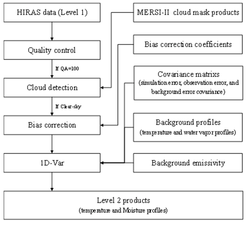
3. HIRAS Atmospheric Sounding System (HASS)

The HASS algorithm consists of four modules, as summarized below:

• A preliminary input quality control and the acquisition of various lookup tables;
• A cloud detection module using MERSI-II visible and infrared observations;
• An angle-dependence bias correction module for measurement spectrum;
• The infrared physical retrieval using 1D-Var.

Figure 3 describes the complete flow diagram of the HASS algorithm. The description of the forward model, lookup tables, cloud detection, bias correction, and 1D-Var algorithm are provided in this section.

3.1. Forward Model

A fast and accurate radiative transfer model is the key to physical retrieval methodology. In this study, the community radiative transfer model (CRTM) was employed, which was developed by the U.S. Joint Center for Satellite Data Assimilation in the early 2000s [29,30] and is a sensor-based radiative transfer model. Based on methods proposed by McMillin and Fleming [31], we developed a fast transmittance model for HIRAS in CRTM. The performance of the HIRAS fast transmittance model can be seen in a previous report [32].

3.2. Lookup Tables

In the HASS algorithm, the lookup tables consist of the background temperature and water vapor profiles, background emissivity, observation and background error matrix, and bias correction coefficients.

The background profiles and their background covariance (see Figure 4a–c) were inherited from MIRS, which represent the mean state of climatological databases and their cross-correlations among the state vectors, and are generated using the European Center for Medium-Range Weather Forecasts (ECMWF) 60-layer sample dataset, the ECMWF analyses, and the model output fields from the Penn State/NCAR Mesoscale Model 5 [33].

The background emissivity, observation error, and bias correction coefficients depend on the simulated spectrum of matched clear-sky analysis dataset between the HIRAS and ERA5 data. The emissivity for a rough sea surface was calculated by an improved model [34]. The average emissivity for every selected channel can be seen in Figure 4d. The observation error is composed of the instrument error and the forward model error. The instrument error (see Figure 5a) is extracted from the theoretical noise equivalent differential temperature, while the forward model error (see Figure 5b) is calculated by the statistical analysis of differences between the observed spectrum and simulated spectrum [35]. For simplicity, the observation error matrix was assumed to be a diagonal matrix. The detail of the bias correction coefficients can be found in Section 3.4.

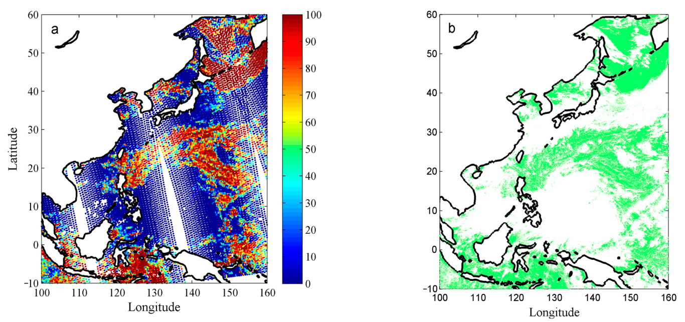
3.3. Cloud Detection

Cloud has a strong effect on infrared radiance [36]. In order to minimize the impact of cloud, only data under clear-sky conditions are used. A cloud detection method has been built by using the difference of SW infrared (4.3 µm) and LW infrared (15 µm) CO₂ bands [37], however, we did not use this method because none of the SW infrared channels in HIRAS were chosen in this study. Instead, we used a collocated HIRAS and MERSI-II scheme for cloud detection. MERSI-II has a synchronous measurement of 16 visible and near-infrared wavebands and nine infrared wavebands with HIRAS, and has high accuracy cloud mask products similar to VIIRS [38,39]. The cloud-detection method consists of two main steps:

• Collocating the geographical coordinates of HIRAS and MERSI-II.
• Calculating the clear fraction of each HIRAS pixel according to the ratio of clear MERSI-II pixels in all of the MERSI-II pixels located in this HIRAS pixel.

In order to evaluate the feasibility of this cloud detection method, a case on 12 September 2018 is displayed in Figure 6. The left-hand panel is the clear fraction of HIRAS pixels, and the right-hand panel is the MERSI-II cloud mask products. The results showed that the areas of high clear fraction in HIRAS and clear-sky in MERSI-II had a good consistency. For more reliable retrieval, only HIRAS pixels with a 100% clear fraction were selected in this study.

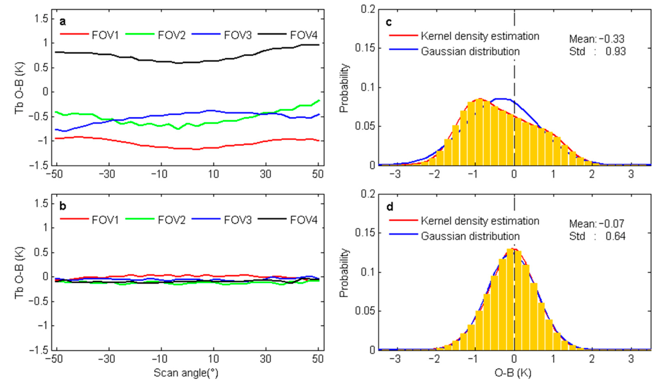
3.4. Bias Correction

All physical methods are based on the assumption that observation errors between the observed radiance and simulated radiance are unbiased and Gaussian [40]. In fact, the observation errors are always biased and non-Gaussian because of the approximate calculation of simulated radiance. Therefore, this bias should be corrected. The research shows that that satellite radiance biases always varied with time, geographic location, satellite zenith angle, and scene temperature [41]. Currently, we only considered the angle-dependent biases in this study. Figure 7 shows the mean bias variation and the probability density distribution of biases at 688.125 cm⁻¹ before and after bias correction. The results show that the original bias distribution is asymmetric along the scan angle, indicating a significant angle-dependent bias for this channel. After bias correction, the mean bias is close to zero, and the bias distribution is more unbiased and Gaussian. It is worth noting that the mean bias variation of the four FOVs showed significant differences and a similar situation occurred in their forward model errors. Thus, the four FOVs should be treated independently in the retrieval.

3.5. 1D-Var Algorithm

The earlier 1D-Var method was mainly applied to data assimilation in numerical weather prediction models [42], but it has been extended to the retrieval of atmospheric profiles from microwave and infrared instruments [43].

The 1D-Var algorithm in this work was developed based on the Microwave Integrated Retrieval System (MIRS) and Microwave Remote Sensing Testbed (MRT), which have been proven to perform well in retrieving the atmospheric temperature and moisture profiles from the Advanced Microwave Sounding Unit (AMSU) and Advanced Technology Microwave Sounder (ATMS), respectively [6,44,45]. The 1D-Var algorithm is performed by minimizing the cost function J, which can be expressed as

$$J=\frac{1}{2}{\left(x-x^b\right)}^T\times B^{-1}\times \left(x-x^b\right)+\frac{1}{2}{\left(H\left(x\right)-I\right)}^T\times E^{-1}\times \left(H\left(x\right)-I\right)$$

where x and x^b are the retrieval and background state vectors, and H(x) and I represent the simulated radiance vectors and observed radiance vectors, respectively. B is the background error covariance matrix, and E is the observation error covariance matrix. The superscript T and −1 indicate the transpose and inverse of a matrix. The first term represents the penalty for departing from a priori information, while the second term indicates the same, but from the measurements. Assuming the forward operator is locally linear, the following iteration can minimize the cost function:

$$\Delta x_{n+1}=\left[{\left(B^{-1}+K_n^T{E}^{-1}{K}_n\right)}^{-1}{K}_n^T{E}^{-1}\right]\left[I^0-H\left(x_n\right)+K_n\Delta x_n\right]$$

where Δx_n and Δx_n+1 represent the departure from the background vectors at iteration index n and n + 1, respectively. K is the Jacobian of H(x_n) with respect to x_n. A detailed flowchart of the 1D-Var algorithm is provided in Figure 8.

The minimization process was performed in the EOF space in this study, which means that the state vectors will be projected back and forth between the geophysical space and the reduced EOF space at every iteration [6]. Note that only a few major eigenvectors/eigenvalues are kept in our retrieval process in order to reduce the unexpected instability and save iteration times. For every state vector, the specific number of eigenvectors/eigenvalues are determined based on how many channels are sensitive to that parameter. In this study, 11 and 20 EOFs were considered for the temperature and humidity retrievals, respectively. Statistically, the average number of iterations for gaining convergence was about 2–3, and those profiles that did not converge after five iterations were marked as questionable profiles and were not included in our assessment.

4. HIRAS Atmospheric Sounding System (HASS)

In order to assess the performance of the 1D-Var algorithm, extensive and ongoing validation is needed. A group of retrieval experiments using the HIRAS hyperspectral data in June, August, September, November and December 2018, and February, March and May 2019, was performed. Due to the lack of matching sounding data when satellite passing in the Western Pacific, ERA5 reanalysis data with a horizontal resolution of 0.25 × 0.25° and vertical resolution of 91 levels as well as the radio occultation (RO) observational data from multiple satellites (including COSMIC, KOMPSAT-5, Metop-A, Metop-B, PAZ, TanDEM-X and TerraSAR-X) were used to validate the precision and accuracy of the HASS algorithm [46,47]. In these experiments, only data under clear-sky conditions and over ocean located in the rectangular region (100°–160°E, 10°S–60°N) were retrieved, to reduce the effects of cloud, surface emissivity, and the geographic-dependent biases. In comparison, the temperature and moisture profiles from ERA5 and RO were assumed as the truth, and the standard deviation error (RMSE) and bias between the retrieval results and valid profiles were calculated. Note that the unit of moisture in the retrieval algorithm is the water vapor mixing ratio (g/kg). To facilitate the comparison of the moisture retrieval results, the water vapor mixing was converted to relative humidity.

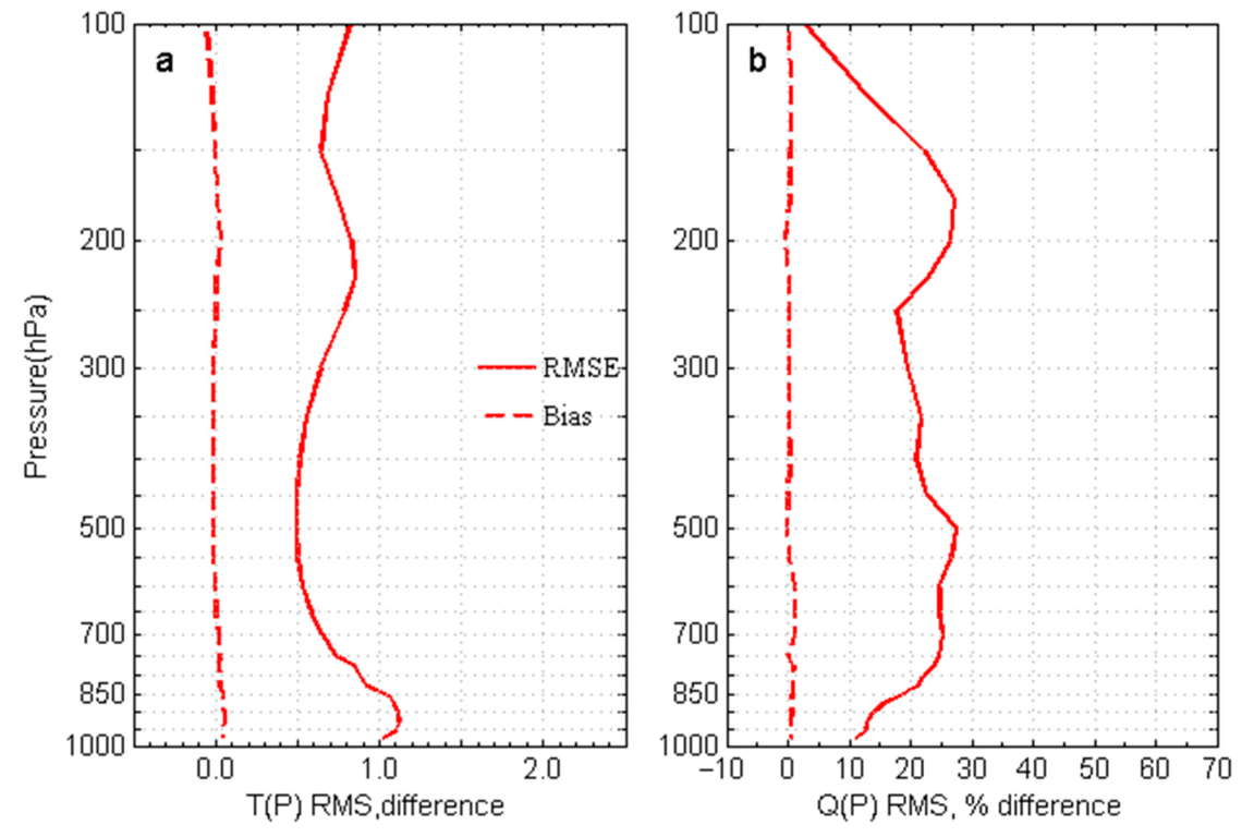
4.1. Validation with ERA5 Reanalysis Data

To minimize the mismatch error between the retrieval results and ERA5 reanalysis data, a stringent spatiotemporal collocation criterion with a temporal difference ≤15 min and spatial distance ≤8 km was applied. Finally, 106,334 samples under clear-sky conditions were used for the retrieval experiments, and the spatial distribution of the density, defined as the number of samples per 100 km², of the retrieval samples and their latitudinal counts are shown in Figure 9. It can be seen that high latitudes had fewer samples than the middle and low latitudes due to the small sea area, and the samples in the middle and low latitudes were relatively well-distributed. Figure 10 shows the RMSE and bias of the temperature and relative humidity profiles between the retrieval results and the ERA5 data. The absolute bias of temperature in the layer above 700 hPa was less than 0.1 K and increased to 0.2 K at 950 hPa, while the bias of relative humidity varied between −3.0% and 1.7%. The RMSE of temperature was about 1 K between 300 hPa and 600 hPa and increased upward and downward, reaching a maximum value of 1.8 K at around 900 hPa. The minimum RMSE of relative humidity was 18.0% at 950 hPa, after which it increased with decreasing pressure, and the maximum amount was 53.4% at around 175 hPa. This may be attributable to the fact that the weighting functions of the water vapor channels were concentrated below 300 hPa (Figure 2d), leading to an increasing RMSE above this level. For better accuracy assessment, the whole atmosphere was divided into three broad layers—the lower level (600–1000 hPa), middle level (300–600 hPa), and upper level (100–300 hPa). The RMSE of temperature and relative humidity for the three broad layers were 1.5 K, 1.0 Km and 1.3 K, and 22.3%, 33.2%, and 38.5%, respectively (displayed in

Table 2. The RMSE and bias of temperature and relative humidity between the retrieval results and ERA5 data in three broad layers.

	Layer Range
	Surface to 600 hPa	600 hPa to 300 hPa	300 hPa to 100 hPa
Temperature (K)	1.5	1.0	1.3
Moisture (%)	22.3	33.2	38.5

). The uncertainty was close to the combined infrared and microwave inversion in AIRS/AMSU algorithm and slightly worse than the inversion in NUCAPS, but still better than the JPSS Level 1 performance requirements for the temperature and moisture profiles [16,48].

To further evaluate the performance of the 1D-Var algorithm, Figure 11 shows the RMSE and bias of the temperature and relative humidity profiles between the retrieval results and the ERA5 data for different FOVs. Although the vertical structures of RMSE were similar, there were still differences of about 0.3 K in temperature and 2.7% in relative humidity between them at the lower level (displayed in

Table 3. The mean RMSE of the temperature and relative humidity between the retrieval results and the ERA5 data for different FOVs in three broad layers.

		Layer Range
		Surface to 600 hPa	600 hPa to 300 hPa	300 hPa to 100 hPa
Temperature (K)	FOV1	1.5	1.0	1.2
	FOV2	1.3	1.0	1.3
	FOV3	1.3	0.9	1.2
	FOV4	1.6	1.0	1.3
Moisture (%)	FOV1	22.6	33.5	38.6
	FOV2	21.1	31.8	37.7
	FOV3	21.2	31.9	38.2
	FOV4	23.8	34.7	39.0

). This FOV difference can also be spotted in the bias distribution. FOV2 and FOV3 tend to have better retrieval results, with the RMSE and bias lower than that from FOV1 and FOV4, especially below mid-troposphere levels. These results indicate that a slight independent post-processing correction is still needed for different FOVs.

Geographic-dependent and temperature-dependent biases have not been applied in the bias correction of satellite radiance, and fixed background profiles are used for the algorithm input. These factors may cause some spatial retrieval errors. To evaluate their effects on the retrieval results, Figure 12 shows the RMSE and bias of the temperature and relative humidity profiles between the retrieval results and ERA5 data in different latitudinal bands. The results at high latitude (40°–60°N) are not shown in Figure 6 due to the decrease in sample size. The results showed that the RMSE and bias differences among the latitudinal bands were higher than those among the FOVs (displayed in

Table 4. The mean RMSE and bias of temperature and relative humidity between the retrieval results and ERA5 data in different latitudinal bands in three broad layers.

		Layer Range
		Surface to 600 hPa	600 hPa to 300 hPa	300 hPa to 100 hPa
Temperature (K)	0°–10°N	1.2	0.9	1.1
	10°–20°N	1.3	1.0	1.1
	20°–30°N	1.4	1.0	1.2
	30°–40°N	1.5	1.0	1.4
Moisture (%)	0°–10°N	15.8	26.8	35.4
	10°–20°N	20.4	35.9	38.4
	20°–30°N	23.7	36.0	40.2
	30°–40°N	26.7	33.0	39.5

), with the temperature RMSE differences reaching about 0.5 K at 950 hPa and the relative humidity RMSE differences about 15.0% at around 800 hPa. Moreover, the RMSE of the temperature and relative humidity increased with the increasing latitude. These variations indicate that geographic-dependent and temperature-dependent biases and fixed background profiles have essential effects on the retrieval results when climatological profiles are used as the first guess.

4.2. Validation with GNOS RO Data

The collocation criterion of the RO observational data is relaxed (due to the sparseness of samples) to a time difference of ≤2 h and a horizontal spatial separation of <200 km. Following this, 867 samples under clear-sky conditions were selected in this study, and the spatial distribution of samples and their latitudinal counts are shown in Figure 13. Figure 14 shows the RMSE and bias of the temperature and relative humidity profiles between the retrieval results and the RO data. Compared with the ERA5 data validation, the RMSE and bias of temperature exhibited a significant increase, with the RMSE below 125 hPa varying from 1.5 K to 2.1 K and the bias range increasing to −0.7 K and 1.6 K. The RMSE of relative humidity between 200 hPa and 600 hPa also increased. The mean RMSE of the temperature and relative humidity for the three broad layers were 1.7 K, 1.8 K, and 1.9 K, and 28.2%, 53.6%, and 43.7%, respectively (displayed in

Table 5. The RMSE and bias of the temperature and relative humidity between the retrieval results and ERA5 data in three broad layers.

	Layer Range
	Surface to 600 hPa	600 hPa to 300 hPa	300 hPa to 100 hPa
Temperature (K)	1.7	1.8	1.9
Moisture (%)	28.2	53.6	43.7

). Compared to Table 2, the maximal RMSE increase in the temperature and relative humidity were both in the middle level, at 0.8 K and 20.4%, respectively.

5. Conclusions

This paper reports the development of the HASS algorithm for the retrieval of atmospheric temperature and moisture profiles based on HIRAS hyperspectral observations. The ‘information entropy’ method was used to select 67 temperature channels, 177 moisture channels, and 30 surface channels. Furthermore, climatological databases were used as the first guess profiles, which can reflect the greater information of satellite observation. A group of retrieval experiments based on the HIRAS observations in June, August, September, November, and December 2018, and February, March and May 2019 were independently performed for different FOVs. The ERA5 reanalysis data and RO observational data were used to perform the assessment. The results showed that this algorithm performed excellently overall, as verified by the ERA5 data, with the RMSE of the temperature and relative humidity for three broad layers being 1.5 K, 1.0 K, and 1.3 K, and 22.3%, 33.2% and 38.5%, respectively. The temperature results were better than those from the AIRS Science Team Version 5 retrieval algorithm and other retrieval algorithms [49,50,51]. However, the corresponding values increased to 1.7 K, 1.8 K, and 1.9 K, and 28.2%, 53.6%, and 43.7%, respectively, in the RO data verification, which may be caused by a larger temporal and spatial matching error. It is worth noting that the RMSE and bias varied with the FOV and latitudinal band, which indicates that the current bias correction method and background profiles still have deficiencies. Furthermore, a sensitivity test using ERA5 profiles as the first guess was performed, and the bias and RMSE of the temperature and relative humidity were significantly reduced (shown in Figure 15 and

Table 6. The RMSE and bias of the temperature and relative humidity between the retrieval results and ERA5 data in three broad layers when the ERA5 data were used as the first guess.

	Layer Range
	Surface to 600 hPa	600 hPa to 300 hPa	300 hPa to 100 hPa
Temperature (K)	0.9	0.5	0.8
Moisture (%)	19.9	23.1	18.7

), which reflects the influence of the prior profile on inversion to some extent.

According to the analysis above, our current HASS algorithm has shown great potential in the atmospheric retrievals of FY-3D/HIRAS. Nonetheless, the following work should be carried out in the future toward an inversion with higher precision. First, an independent post-processing correction should be applied to different FOVs. Second, geographic- and temperature-dependent bias correction and space-adaptive background profiles should be used instead of the current angle-dependent bias correction and fixed background profiles.

References

1. Güldner, J.; Spänkuch, D. Remote Sensing of the Thermodynamic State of the Atmospheric Boundary Layer by Ground-Based Microwave Radiometry. J. Atmos. Ocean. Technol. 2001, 18, 925–933. [Google Scholar] [CrossRef] [Green Version]
2. Rodgers, C.D. Series on Atmospheric Oceanic and Planetary Physics. In Inverse Methods for Atmospheric Sounding–Theory and Practice, 2nd ed.; World Science: Singapore, 2000. [Google Scholar]
3. Susskind, J.; Barnet, C.; Blaisdell, J.; Iredell, L.; Keita, F.; Kouvaris, L. Early results from AIRS/AMSU/HSB. In Proceedings of the SPIE Annual Meeting, San Diego, CA, USA, 3 August 2003. [Google Scholar] [CrossRef] [Green Version]
4. Goldberg, M.; Qu, Y.; McMillin, L.; Wolf, W.; Zhou, L.; Divarkarla, M. Real time operational products from AIRS. Opt. Remote Sens. 2003. [Google Scholar] [CrossRef] [Green Version]
5. Liu, Q.H.; Weng, F.Z. A microwave polarimetric two-stream radiative transfer model. J. Atmos. Sci. 2002, 59, 2396–2402. [Google Scholar] [CrossRef]
6. Seemann, S.W.; Li, J.; Menzel, W.P.; Gumley, L.E. Operational Retrieval of Atmospheric Temperature, Moisture, and Ozone from MODIS Infrared Radiances. J. Appl. Meteor. 2003, 42, 1072–1091. [Google Scholar] [CrossRef]
7. Zhang, L.; Qiu, C.; Huang, J. A three-dimensional satellite retrieval method for atmospheric temperature and moisture profiles. Adv. Atmos. Sci. 2008, 25, 897–904. [Google Scholar] [CrossRef]
8. Milstein, A.B.; Blackwell, W.J. Neural network temperature and moisture retrieval algorithm validation for AIRS/AMSU and CrIS/ATMS. J. Geophys. Res. Atmos. 2016, 121, 1414–1430. [Google Scholar] [CrossRef] [Green Version]
9. Thompson, O.E.; Eom, J.K.; Wagenhofer, J.R. On the Resolution of Temperature Profile Finestructure by the NOAA Satellite Vertical Temperature Profile Radiometer. Mon. Weather Rev. 1976, 104, 117–126. [Google Scholar] [CrossRef] [Green Version]
10. High Resolution Infrared Radiation Sounder/Mod 2 (HIRS/2). Available online: https://ntrs.nasa.gov/api/citations/19800024547/downloads/19800024547.pdf (accessed on 22 June 2021).
11. Aumann, H.H.; Chahine, M.T.; Gautier, C.; Goldberg, M.D.; Kalnay, E.; McMillin, L.M.; Susskind, J. AIRS/AMSU/HSB on the aqua mission: Design, science objectives, data products, and processing systems. IEEE Trans. Geosci. Remote Sens. 2003, 41, 253–264. [Google Scholar] [CrossRef] [Green Version]
12. Klaes, K.D.; Cohen, M.; Buhler, Y.; Schlussel, P.; Munro, R.; Luntama, J.P.; Schmetz, J. An introduction to the EUMETSAT Polar System. Bull. Am. Meteorol. Soc. 2007, 88, 1085–1096. [Google Scholar] [CrossRef]
13. Smith, A.; Atkinson, N.; Bell, W.; Doherty, A. An initial assessment of observations from the Suomi-NPP satellite: Data from the Cross-track Infrared Sounder (CrIS). Atmos. Sci. Lett. 2015, 16, 260–266. [Google Scholar] [CrossRef]
14. High Resolution GLAS on the MCIDAS. Available online: https://ntrs.nasa.gov/citations/19840013994 (accessed on 22 June 2021).
15. Li, J.; Wolf, W.; Menzel, W.; Zhang, W.; Huang, H.-L.; Achtor, T. Global Soundings of the Atmosphere from ATOVS Measurements: The Algorithm and Validation. J. Appl. Meteorol. 2000, 39, 1248–1268. [Google Scholar] [CrossRef]
16. Susskind, J.; Barnet, C.; Blaisdell, J.; Iredell, L.; Keita, F.; Kouvaris, L.; Chahine, M. Accuracy of geophysical parameters derived from Atmospheric Infrared Sounder/Advanced Microwave Sounding Unit as a function of fractional cloud cover. J. Geophys. Res. -Atmos. 2006, 111, D09S17. [Google Scholar] [CrossRef] [Green Version]
17. Gambacorta, A.; Nalli, N.R.; Tan, C.; Iturbide-Sanchez, F.; Wilson, M.; Zhang, K.; Goldberg, M. Status of the NPP and J1 NOAA Unique Combined Atmospheric Processing System (NUCAPS): Recent algorithm enhancements geared toward validation and near real time users applications. In Proceedings of the AGU Fall Meeting, San Francisco, CA, USA, 12–16 December 2016. [Google Scholar]
18. Rosenkranz, P.W. Retrieval of water vapor from AMSU-A and AMSU-B measurements. In Proceedings of the IEEE 2000 International Geoscience and Remote Sensing Symposium, Honolulu, HI, USA, 24–28 July 2000. [Google Scholar] [CrossRef]
19. Goldberg, M.; Barnet, C.; Wolf, W.; Zhou, L.; Divakarla, M. Distributed real-time operational products from AIRS. In Proceedings of the SPIE Atmospheric and Environmental Remote Sensing Data Processing and Utilization: An End-to-End System Perspective, Denver, CO, USA, 4–6 August 2004. [Google Scholar] [CrossRef]
20. Chahine, M. Remote Sounding of Cloudy Atmospheres. I. The Single Cloud Layer. J. Atmos. Sci. 1974, 31, 233–243. [Google Scholar] [CrossRef] [Green Version]
21. Zhang, P.; Chen, L.; Di, X.; Xu, Z. Recent progress of Fengyun meteorology satellites. China J. Space Sci. 2018, 38, 788–796. [Google Scholar]
22. Lee, L.; Zhang, P.; Qi, C.L.; Hu, X.Q.; Gu, M.J. HIRAS noise performance improvement based on principal component analysis. Appl. Opt. 2019, 58, 5506–5515. [Google Scholar] [CrossRef]
23. Qi, C.; Yang, Z.; Zhang, P.; Wu, C.; Hu, X.; Xu, H.; Shao, C. High Spectral Infrared Atmospheric Sounder (HIRAS): System Overview and On-Orbit Performance Assessment. IEEE Trans. Geosci. Remote Sens. 2020, 58, 4335–4352. [Google Scholar] [CrossRef]
24. Wu, C.; Qi, C.; Hu, X.; Gu, M.; Yang, T.; Xu, H.; Zhang, P. FY-3D HIRAS Radiometric Calibration and Accuracy Assessment. IEEE Trans. Geosci. Remote Sens. 2020, 58, 3965–3976. [Google Scholar] [CrossRef]
25. Han, Y.; Revercomb, H.; Cromp, M.; Gu, D.G.; Johnson, D.; Mooney, D.; Zavyalov, V. Suomi NPP CrIS measurements, sensor data record algorithm, calibration and validation activities, and record data quality. J. Geophys. Res. Atmos. 2013, 118, 12734–12748. [Google Scholar] [CrossRef]
26. Rodgers, C.D. Information content and optimisation of high spectral resolution remote measurements. Adv. Space Res. 1998, 21, 361–367. [Google Scholar] [CrossRef]
27. Rabier, F.; Fourrié, N.; Chafäi, D.; Prunet, P. Channel selection methods for Infrared Atmospheric Sounding Interferometer radiances. Q. J. R. Meteorol. Soc. 2002, 128, 1011–1027. [Google Scholar] [CrossRef] [Green Version]
28. Collard, A.D. Selection of IASI channels for use in numerical weather prediction. Q. J. R. Meteorol. Soc. 2007, 133, 1977–1991. [Google Scholar] [CrossRef]
29. Weng, F.; Liu, Q. Satellite Data Assimilation in Numerical Weather Prediction Models. Part I: Forward Radiative Transfer and Jacobian Modeling in Cloudy Atmospheres. J. Atmos. Sci. 2003, 60, 2633–2646. [Google Scholar] [CrossRef]
30. Weng, F.Z. Advances in radiative transfer modeling in support of satellite data assimilation. J. Atmos. Sci. 2007, 64, 3799–3807. [Google Scholar] [CrossRef]
31. McMillin, L.; Fleming, H. Atmospheric transmittance of an absorbing gas—A computationally fast and accurate transmittance model for absorbing gases with constant mixing ratios in inhomogeneous atmospheres. Appl. Opt. 1976, 15, 358. [Google Scholar] [CrossRef]
32. Weng, F.; Yu, X.; Duan, Y.; Yang, J.; Wang, J. Advanced Radiative Transfer Modeling System (ARMS): A New-Generation Satellite Observation Operator Developed for Numerical Weather Prediction and Remote Sensing Applications. Adv. Atmos. Sci. 2020, 37, 131–136. [Google Scholar] [CrossRef] [Green Version]
33. Boukabara, S.A.; Garrett, K.; Chen, W.C.; Iturbide-Sanchez, F.; Grassotti, C.; Kongoli, C.; Meng, H. MiRS: An All-Weather 1DVAR Satellite Data Assimilation and Retrieval System. IEEE Trans. Geosci. Remote Sens. 2011, 49, 3249–3272. [Google Scholar] [CrossRef]
34. Wu, X.; Smith, W.L. Emissivity of rough sea surface for 8 13 m: Modeling and verification. Appl. Opt. 1997, 36, 2609–2619. [Google Scholar] [CrossRef]
35. Crow, W. Estimating Model and Observation Error Covariance Information for Land Data Assimilation Systems. In Land Surface Observation, Modeling and Data Assimilation; Liang, S., Ed.; Springer: Berlin/Heidelberg, Germany, 2012; pp. 171–205. [Google Scholar]
36. Geer, A.J.; Migliorini, S.; Matricardi, M. All-sky assimilation of infrared radiances sensitive to mid- and upper-tropospheric moisture and cloud. Atmos. Meas. Tech. 2019, 12, 4903–4929. [Google Scholar] [CrossRef] [Green Version]
37. Lin, L.; Zou, X.L.; Weng, F.Z. Combining CrIS double CO2 bands for detecting clouds located in different layers of the atmosphere. J. Geophys. Res. Atmos. 2017, 122, 1811–1827. [Google Scholar] [CrossRef]
38. Qu, J.; Yan, J.; Xxue, J.; Guo, X. Research on the cloud detection model of FY3D/MERSI and EOS/MODIS based on deep learning. J. Meteorol. Environ. 2019, 35, 87–93. [Google Scholar]
39. Kopp, T.J.; Thomas, W.; Heidinger, A.K.; Botambekov, D.; Frey, R.A.; Hutchison, K.D.; Reed, B. The VIIRS Cloud Mask: Progress in the first year of S-NPP toward a common cloud detection scheme. J. Geophys. Res. Atmos. 2014, 119, 2441–2456. [Google Scholar] [CrossRef]
40. Weng, F.; Zou, X.; Wang, X.; Yang, S.; Goldberg, M.D. Introduction to Suomi national polar-orbiting partnership advanced technology microwave sounder for numerical weather prediction and tropical cyclone applications. J. Geophys. Res. Atmos. 2012, 117. [Google Scholar] [CrossRef]
41. Saunders, R.W.; Blackmore, T.A.; Candy, B.; Francis, P.N.; Hewison, T.J. Monitoring Satellite Radiance Biases Using NWP Models. IEEE Trans. Geosci. Remote Sens. 2013, 51, 1124–1138. [Google Scholar] [CrossRef]
42. Weng, F.Z.; Zhu, T.; Yan, B.H. Satellite data assimilation in numerical weather prediction models. Part II: Uses of rain-affected radiances from microwave observations for hurricane vortex analysis. J. Atmos. Sci. 2007, 64, 3910–3925. [Google Scholar] [CrossRef] [Green Version]
43. Liu, Q.H.; Weng, F.Z. One-dimensional variational retrieval algorithm of temperature, water vapor, and cloud water profiles from Advanced Microwave Sounding Unit (AMSU). IEEE Trans. Geosci. Remote Sens. 2005, 43, 1087–1095. [Google Scholar]
44. Han, Y.; Weng, F.Z. Remote Sensing of Tropical Cyclone Thermal Structure from Satellite Microwave Sounding Instruments: Impacts of Optimal Channel Selection on Retrievals. J. Meteorol. Res. 2018, 32, 804–818. [Google Scholar] [CrossRef]
45. Hu, H.; Weng, F.Z.; Han, Y.; Duan, Y.H. Remote Sensing of Tropical Cyclone Thermal Structure from Satellite Microwave Sounding Instruments: Impacts of Background Profiles on Retrievals. J. Meteorol. Res. 2019, 33, 89–103. [Google Scholar] [CrossRef]
46. Palmer, P.I.; Barnett, J.J.; Eyre, J.R.; Healy, S.B. A nonlinear optimal, estimation inverse method for radio occultation measurements of temperature, humidity, and surface pressure. J. Geophys. Res. Atmos. 2000, 105, 17513–17526. [Google Scholar] [CrossRef] [Green Version]
47. Zhang, W.; Zhang, H.; Liang, H.; Lou, Y.; Cai, Y.; Cao, Y.; Liu, W. On the suitability of ERA5 in hourly GPS precipitable water vapor retrieval over China. J. Geod. 2019, 93, 1897–1909. [Google Scholar] [CrossRef]
48. Nalli, N.; Gambacorta, A.; Liu, Q.; Barnet, C.; Tan, C.; Iturbide-Sanchez, F.; Morris, V. Validation of Atmospheric Profile Retrievals From the SNPP NOAA-Unique Combined Atmospheric Processing System. Part 1: Temperature and Moisture. IEEE Trans. Geosci. Remote Sens. 2017, 56, 180–190. [Google Scholar] [CrossRef]
49. Susskind, J.; Blaisdell, J.M.; Iredell, L.; Keita, F. Improved Temperature Sounding and Quality Control Methodology Using AIRS/AMSU Data: The AIRS Science Team Version 5 Retrieval Algorithm. IEEE Trans. Geosci. Remote Sens. 2011, 49, 883–907. [Google Scholar] [CrossRef] [Green Version]
50. Smith, W.L.; Weisz, E.; Kireev, S.V.; Zhou, D.K.; Li, Z.L.; Borbas, E.E. Dual-Regression Retrieval Algorithm for Real-Time Processing of Satellite Ultraspectral Radiances. J. Appl. Meteorol. Climatol. 2012, 51, 1455–1476. [Google Scholar] [CrossRef]
51. Zhang, K.; Wu, C.Q.; Li, J. Retrieval of Atmospheric Temperature and Moisture Vertical Profiles from Satellite Advanced Infrared Sounder Radiances with a New Regularization Parameter Selecting Method. J. Meteorol. Res. 2016, 30, 356–370. [Google Scholar] [CrossRef]
Figure 1. The HIRAS ground footprints from (a) one single scan line, (b) the central FORs of the scan line.
Remotesensing 14 03882 g001
Figure 2. (a) The blacklist (grey shaded area) and (b) the perturbations of temperature, water vapor, ozone, and surface temperature in the HIRAS LW and MW bands. (c) The wavenumbers and (d) the weighting functions of all of the selected channels. Red, blue, green, and pink represent the temperature, water vapor, surface temperature and ozone, respectively.
Remotesensing 14 03882 g002
Figure 3. The complete flow chart of the HASS algorithm.
Remotesensing 14 03882 g003
Figure 4. The Temperature (a) and water vapor (b) background profiles as well as the covariance matrix (c) used in the 1D-Var algorithm. Note that the covariance matrix has been converted to a correlation matrix to highlight the connection among variables. (d) The background emissivity for all of the selected channels.
Remotesensing 14 03882 g004
Figure 5. The instrument error (a) and simulation error (b) of the selected channels.
Remotesensing 14 03882 g005
Figure 6. The spatial distribution of the (a) clear fractions within HIRAS FOVs, and the (b) MERSI-II cloud mask products on 12 September 2018. Green in the right-hand panel represents clear-sky.
Remotesensing 14 03882 g006
Figure 7. The mean variation of biases with a scan angle of four FOVs (a,c), and the probability density distribution of biases at 688.125 cm−1 (b,d) before and after bias correction.
Remotesensing 14 03882 g007
Figure 8. A flow chart of the 1D-VAR algorithm.
Remotesensing 14 03882 g008
Figure 9. (a) The spatial distribution of the density of the retrieval samples (/100 km2) between the HIRAS and ERA5 data. (b) The count of retrieval samples in the 1° latitudinal bands. (c) The count of retrieval samples in the 10° latitudinal bands.
Remotesensing 14 03882 g009
Figure 10. The RMSE and bias of temperature (a) and relative humidity (b) profiles between the retrieval results and ERA5 data.
Remotesensing 14 03882 g010
Figure 11. The RMSE and bias of temperature (a) and relative humidity (b) profiles between the retrieval results and the ERA5 data for different FOVs.
Remotesensing 14 03882 g011
Figure 12. The RMSE and bias of the temperature (a) and relative humidity (b) profiles between the retrieval results and ERA5 data in different 10° latitudinal bands.
Remotesensing 14 03882 g012
Figure 13. (a) The spatial distribution of retrieval samples between the HIRAS and RO data. (b) The count of retrieval samples in 10° latitudinal bands.
Remotesensing 14 03882 g013
Figure 14. The RSE and bias of the temperature (a) and relative humidity (b) profiles between the retrieval results and RO data.
Remotesensing 14 03882 g014
Figure 15. The RMSE and bias of the temperature (a) and relative humidity (b) profiles between the retrieval results and ERA5 data when the ERA5 data were used as the first guess.
Remotesensing 14 03882 g015