Analysis of the Influence of Attitude Error on Underwater Positioning and Its High-Precision Realization Algorithm

Abstract

GNSS/INS can provide position, attitude, and velocity (PAV) information for shipborne platforms. However, if the ship has a long-term linear motion or a stationary state, and is under the combined actions of sea surface swells, there will be a situation of sideslip and drift; if the ship is traveling slowly or shaking violently, the attitude calculation will not be completed. In the above situation, the traditional single-antenna GNSS/INS measurement mode is not suitable, and the attitude observability is poor; the heading angle attitude information, especially, will gradually diverge. Unreliable information will directly lead to a significant increase in underwater positioning errors. In this paper, a multi-antenna GNSS/INS combination algorithm is developed and used to provide high-precision PAV information, and is thereby able to obtain high-precision underwater positioning results. The experimental results show that the method has improved the acquisition of position and velocity in the horizontal direction and the accuracy of navigation attitude measurement. In particular, the attitude measurement accuracy in the 3 degrees of freedom (DoF) are improved by 10.1% (roll), 8.6% (pitch), and 29.3% (yaw).

1. Introduction

The ocean is an important space for sustainable human development, and ocean security is an important part of national sovereignty [1]. Underwater positioning and navigation are indispensable parts of the development of an integrated PNT (positioning, navigation, and timing) system [2]. Safe navigation for the laying of underwater oil pipelines, prediction of potential marine disasters, and tracking of underwater vehicles/robots are all inseparable from the basic information of one’s position in the deep ocean [3]. GNSS/A (global navigation satellite system—acoustic) technology has been widely used in underwater positioning, which can achieve centimeter-level positioning accuracy [4].

GNSS-A is a technology that can realize the transmission of the reference. Its principle is to use the GNSS technology to complete the calibration and measurement of the surface survey ships/buoys, and then realize the positioning of an underwater target through the measurements of the distances by the acoustic signals. Among them, underwater positioning is to achieve positioning through distance intersection on the basis of measuring the distance between the transducer installed on the ship and the transponder on the seabed. In this process, there are many factors that affect high-precision underwater positioning. For instance, the ranging of acoustic signals requires high-precision time measurement and sound velocity field observation [5]. Systematic errors in hardware may lead to inaccurate timing, while sound velocity measurement errors are among the most important error sources affecting underwater positioning. Sound velocity is a complex function of water temperature, salinity, and pressure, and has temporal and spatial variation characteristics. It is difficult to measure accurately [6]. In addition, to achieve high-precision underwater positioning, high-precision PAV information of the surface ship is necessary. Researchers have discussed the influence of the ship’s attitude measurement error on the accuracy of multi-beam bathymetry [7]. In addition to the attitude error, Jin et al. also considers the coupling effect with the sound ray bending error and deduces the position of the bottom sounding point and the sounding reduction model [8].

GNSS can provide low sampling rate position, velocity, and time information. The performance of real-time kinematic (RTK) positioning technology is affected by the spatial correlation of various errors as the distance increases. Generally, the valid operating distance should not exceed 15 km, so accurate positioning cannot be achieved in the remote sea positioning scenario. PPP (precise point positioning) technology can provide centimeter-level position and velocity information for users in the remote sea [9]. The dual-antenna RTK/PPP receiver of the commercial product ‘Vector VS1000’ can measure the attitude accuracy of 0.01° RMS and supports antenna separations up of 10 m. INS (inertial navigation system) can measure the triaxial accelerations and angular velocities of the platform, with the characteristics of high sampling rate, and is not affected by the environment [10]. However, as the observation time increases, the measurement errors of the individual INS gradually accumulate. After a period of time, the PVA determination results are seriously shifted. Therefore, integrated GNSS/INS navigation and positioning technology has been developed rapidly. It can provide high-precision PVA information and has been widely used in different vehicle/ship/airborne platforms. Due to the complexity of the marine environments, the correlation between the attitude parameters of the ship-borne motion platform caused by the low velocity, large shaking and zero bias parameters of the gyroscope decreases rapidly. The multi-antenna GNSS/INS mode greatly enhances the ability to resist complex environments. It can provide high-precision three-axis attitude of the carrier, and greatly improve the output capability of high-frequency navigation information [11]. The technology of single-antenna GNSS/INS integrated navigation has matured. However, the single-antenna mode ignores the side-slip angle of the carrier and the influence of the carrier motion when the motion is low, so it cannot accurately measure the heading angle, and therefore the application is limited [12]. In the conventional dual-antenna GNSS/INS combined attitude measurement, the differential equation of the Euler angle is mostly used as the state equation. This method is incompatible with the basic model of the GNSS/INS combination and cannot integrate the attitude measurement information synchronously.

The three-antenna-assisted GNSS/INS integrated navigation system cannot only provide position and velocity but also three-dimensional attitude information to cope with the complex and changeable marine environment. It compensates for the attitude of the marine survey measurement platform to improve the acquisition of the platform’s PVA information. At present, the application and discussion of this method are mostly seen in vehicle-mounted land systems; the discussion about ocean observation platforms is poor and the impact on underwater positioning is even less discussed.

2. Materials and Methods

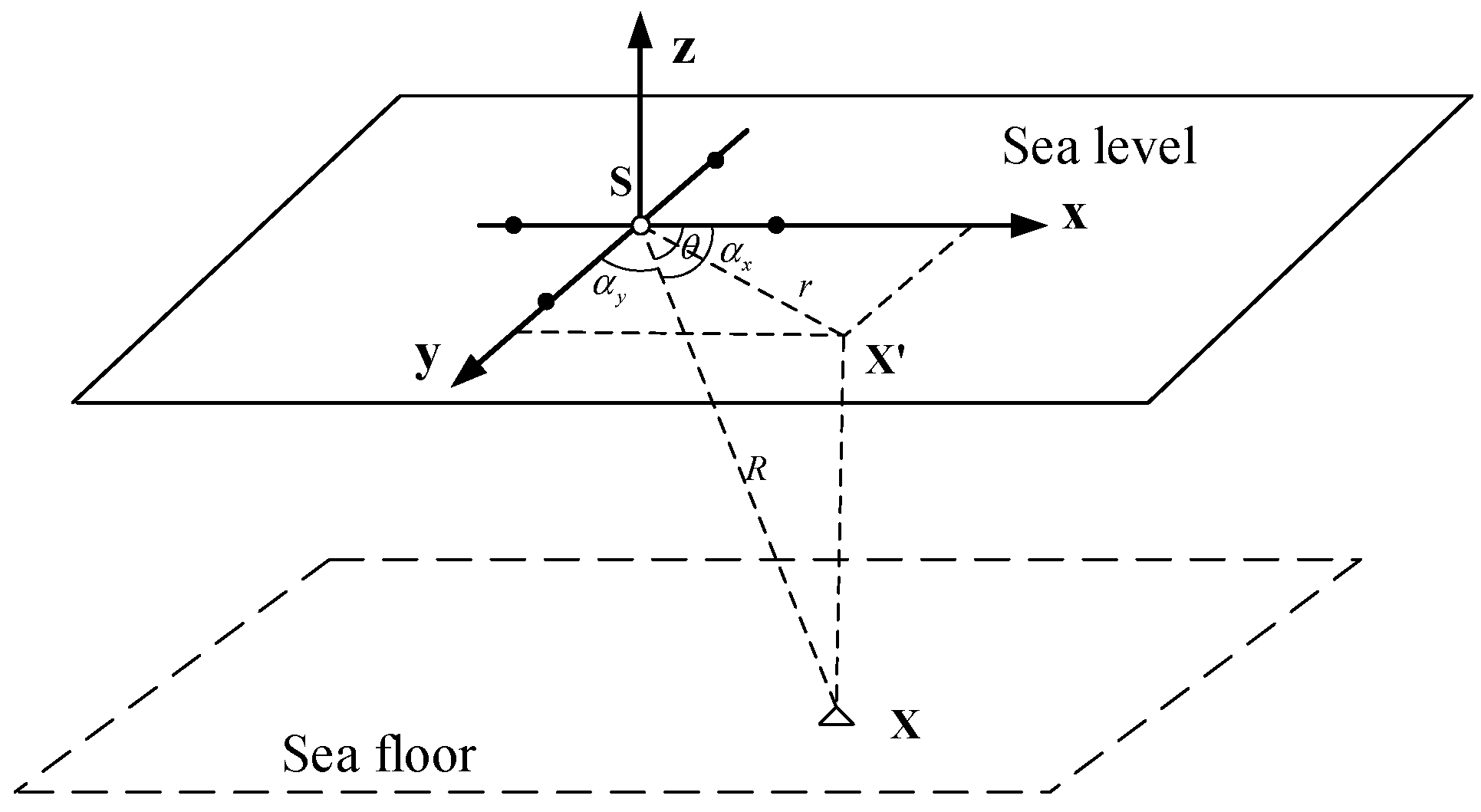
2.1. The Principle of GNSS-A Positioning

GNSS-A technology links GNSS and acoustic positioning methods to accurately co-locate the position of the seafloor datum point [13,14]. As shown in Figure 1, we installed the acoustic array transducer on the bottom of the ship and obtained the position information of the underwater transponder by measuring the phase delay or time delay. This technique is called ultra-short baseline localization (USBL). Its significant advantage is that the hardware is small in size and easy to operate. The GNSS technology can be used to determine their three-dimensional (3D) coordinates. Assuming that the underwater target is located at $\mathrm{X}\left(x,y,z\right)$.

Suppose the target radius vector is $\overline{\mathrm{S}\mathrm{X}}$, and its direction cosine is [15]:

$$\cos {\alpha }_x=\frac{x}{R}$$

(1)

$$\cos {\alpha }_y=\frac{y}{R}$$

(2)

$$R=\sqrt{x^2+y^2+z^2}$$

(3)

where ${\alpha }_x$ is the angle between $\overline{\mathrm{S}\mathrm{X}}$ and the x axis; ${\alpha }_y$ is the angle between $\overline{\mathrm{S}\mathrm{X}}$ and the y axis; and $R$ is the slope distance.

$$\theta ={\tan }^{-1}\frac{\cos {\alpha }_y}{\cos {\alpha }_x}$$

(4)

$$r=\sqrt{x^2+y^2}$$

(5)

$$z=-\sqrt{R^2-r^2}$$

(6)

where $\theta$ is the angle between $\overline{S{X}^{\prime }}$ and the x axis; $r$ is the horizontal slope distance of the target, and $z$ is the depth of the target. Based on the time-delayed measurement observations, we have:

$$\{\begin{array}{c}{\tau }_x=\frac{L\cos {\alpha }_x}{c}\\ {\tau }_y=\frac{L\cos {\alpha }_y}{c}\end{array}$$

(7)

where $c$ is the sound speed. $L$ is the array element spacing. ${\tau }_x$ and ${\tau }_y$ are the time-delayed measurements. Based on the above discussion, the plane position $\left(x,y\right)$ of the target can be calculated estimation with Equation (8):

$$\{\begin{array}{c}x=\frac{c{\tau }_{x}R}{L}\\ y=\frac{c{\tau }_{y}R}{L}\end{array}$$

(8)

Note in particular that the actual observed values are ${\tau }_x$ and ${\tau }_y$. In addition, R is calculated with the transponder time measurement, and the influence of the sound velocity error must be considered in practical application. The acoustic tracing algorithms are commonly used to solve this problem.

Due to the time and space characteristics of the marine environment, especially the complexity of the deep-sea area, the impact of observation noise cannot be ignored. For the USBL positioning system, the interaction of various errors causes its positioning error to diverge after more than a few hundred meters. It is very fast, so the effective positioning distance cannot be far, which affects the application of USBL in deep-sea operations [16]. To improve the positioning accuracy of USBL, the key lies in the analysis and correction of positioning errors.

Similar to GNSS positioning error analysis, the error sources of GNSS-A positioning can be divided into four categories, which can be expressed as:

$${\epsilon }_{GNSS-A}={\epsilon }_{td}+{\epsilon }_{tp}+{\epsilon }_e+{\epsilon }_{other}$$

(9)

where ${\epsilon }_{td}$ is the errors related to the surface transducer, including the positioning error of the GNSS to the surface ship, the attitude error of the ship, etc.; ${\epsilon }_{tp}$ is the errors related to the seafloor transponder, mainly referring to the time measurement system error caused by the hardware; ${\epsilon }_e$ is the errors related to the travel path, and it is the most important one is the error caused by inaccurate sound velocity measurement; and ${\epsilon }_{other}$ is other relevant errors, such as the positioning error caused by the poor geometry of the sea surface control points and the error caused by the observation altitude angle.

2.2. Influence of Sea Surface Control Point Error on Underwater Positioning

From the discussion of the error composition in the previous section, it can be seen that the error associated with the transducer must be discussed and corrected. It is well-known that oceanographic measurements are always carried out in a dynamic environment, and transducer sensors are installed on ships/buoys sailing on the sea surface. The transducer is usually installed on the bottom of the ship by means of fixed connection. Although the initial installation process is relatively complicated, once the installation is completed, it can be positioned and measured at any time [17]. Not only does it eliminate the need for array deployment and recovery during each test, but also improves the system measurement accuracy to a certain extent. The coordinate transformation process is show in Figure 2.

Since the measurement carrier is affected by disturbance factors such as wind, current, and swell, it is inevitable that motions such as roll, pitch, and yaw will occur. This undoubtedly increases the influence of errors on high-precision positioning, so the influence of measurement errors caused by the dynamic effects of the ocean must be considered. The problem of position reduction of the sea surface control point is the common problem that needs to be solved first, that is, the eccentricity problem caused by the inconsistency between the acoustic signal transmitting transducer and the center of the equipment antenna. Under the dynamic effect of the ocean, the position correction will change with the navigation change and swaying amplitude of the measurement carrier, which has obvious time variations [18].

It is assumed that during the positioning process, the origin of the matrix coordinate system is stationary relative to the geodetic coordinate system, and there is a constant deviation $\Delta \mathbf{X}=(\Delta x,\Delta y,\Delta z{)}^T$ between the origins of the two coordinate systems. Then assume that the matrix coordinate system is $oxyz$, and the geodetic coordinate system is $OXYZ$. The matrix first rotates around the Z-axis by $\psi$ (heading angle), then rotates around the Y-axis by $\theta$ (roll angle), and then rotates around the X-axis by $\varphi$ (pitch angle). The positions of the target in the geodetic coordinate system and the matrix coordinate system are $X_E$ and $X_B$, respectively.

The rotation matrix from the ship coordinate system to the earth coordinate system is $R_s^e=f\left(\varphi ,\theta ,\psi \right)$.

$$R_s^e=\left(\begin{array}{ccc}\cos \theta \cos \varphi & \cos \theta \sin \varphi & \sin \theta \\ -\cos {\psi }^{\prime }\sin \varphi -\sin {\psi }^{\prime }\sin \theta \cos \varphi & \cos {\psi }^{\prime }\cos \varphi -\sin {\psi }^{\prime }\sin \theta \sin \varphi & \sin {\psi }^{\prime }\cos \theta \\ \sin {\psi }^{\prime }\sin \varphi -\cos {\psi }^{\prime }\sin \theta \cos \varphi & -\sin {\psi }^{\prime }\cos \varphi -\cos {\psi }^{\prime }\sin \theta \sin \varphi & \cos {\psi }^{\prime }\cos \theta \end{array}\right)$$

(10)

where ${\psi }^{\prime }=ac\sin (\sin \psi /\cos \theta )$. At the same time, we assume that the rotation matrix from the base matrix coordinate system to the ship coordinate system is $R_b^s=f\left(\alpha ,\beta ,\gamma \right)$. Then the coordinates of the target in the geodetic coordinate system $X_E$ is [15]:

$$X_E=X_G+R_s^e\cdot R_b^s\cdot X_B+R_s^e\cdot \Delta X$$

(11)

where $X_G$ is the phase center coordinates of the GNSS antenna.

In fact, the measured target position is often relative to the north coordinate system centered on the array. Therefore, it can be assumed that the origin of the matrix coordinate system is stationary relative to the geodetic coordinates during the measurement process, and the origin of the two coordinate systems is considered to be the same or have a fixed offset, so that only the rotation of the matrix around the coordinate axis is considered.

It can be seen from Equation (11) that the accuracy of GNSS positioning determines whether $X_G$ is accurate. If it has measurement error, it will be directly transmitted to the position error of the transponder in the geodetic coordinate system.

$$\partial X_E=\partial X_G$$

(12)

Due to the influence of the hydroacoustic environment and the sway of the survey ship, the attitude of the underwater system measurement array is not fixed. The real-time attitude of the transducer must be corrected, and the target position measured by the system relative to the transducer coordinate system must be converted to the ship coordinates or even the geodetic coordinates to truly draw the actual position of the underwater target.

From Equation (11), it can be known that the attitude error is related to $R_s^e·R_b^s·X_B$ and $R_s^e·\Delta X$. We assume that:

$$\{\begin{array}{l}{L}_{X_E}={\left(\begin{array}{ccc}{L}_{x_E}& L_{y_E}& L_{z_E}\end{array}\right)}^T=R_s^e·R_b^s·X_B\hfill \\ K_{X_E}={\left(\begin{array}{ccc}{K}_{x_E}& K_{y_E}& K_{z_E}\end{array}\right)}^T=R_s^e·\Delta X\hfill \end{array}$$

(13)

The total differentiation with respect to $L_{x_E}$ is:

$$\Delta L_{x_E}=\frac{\partial L_{x_E}}{\partial \varphi }\Delta \varphi +\frac{\partial L_{x_E}}{\partial \theta }\Delta \theta +\frac{\partial L_{x_E}}{\partial \psi }\Delta \psi$$

(14)

In the same way, we can find the total differential of $L_{y_E},L_{z_E},K_{x_E},K_{y_E},K_{z_E}$. Assume:

$$\Delta {\varphi }^2=\Delta {\theta }^2=\Delta {\psi }^2={\sigma }_{att}^2$$

(15)

The relative errors can be expressed as:

$$\frac{\sqrt{\Delta L_E^2}}{R}=\frac{\sqrt{\Delta L_{x_E}^2+\Delta L_{y_E}^2+\Delta L_{z_E}^2}}{R}=\sqrt{2}·{\sigma }_{att}$$

(16)

$$\frac{\sqrt{\Delta K_E^2}}{R}=\frac{\sqrt{\Delta K_{x_E}^2+\Delta K_{y_E}^2+\Delta K_{z_E}^2}}{R}=\sqrt{2}·\frac{\Delta R}{R}{\sigma }_{att}$$

(17)

Then, the total influence of the ship’s attitude error on the positioning is:

$${\mathsf{\Omega }}_{att}=\frac{\sqrt{\Delta L_E^2}}{R}+\frac{\sqrt{\Delta K_E^2}}{R}=\sqrt{2}\left(1+\frac{\Delta R}{R}\right){\sigma }_{att}$$

(18)

In general, affected by the dynamic effect of the ocean, there are some measurement errors in the position and attitude of the measuring ship, which in turn causes the inaccuracy of the underwater positioning results. Therefore, it is necessary to find a method to improve the accuracy of the PAV information. Below is a multi-antenna assisted GNSS/INS integrated navigation and positioning method, which is expected to effectively improve the PAV accuracy.

This paper discusses the influence of the ship’s PAV information on the positioning of fixed underwater targets. In fact, we still focus on the impact of this information on underwater dynamic target navigation. For example, the navigation of underwater AUV (autonomous underwater vehicle) usually adopts a combination of multi-sensors. A high-precision IMU (inertial measurement unit), DVL (doppler velocity log) and USBL will be installed on the carrier to obtain PAV.

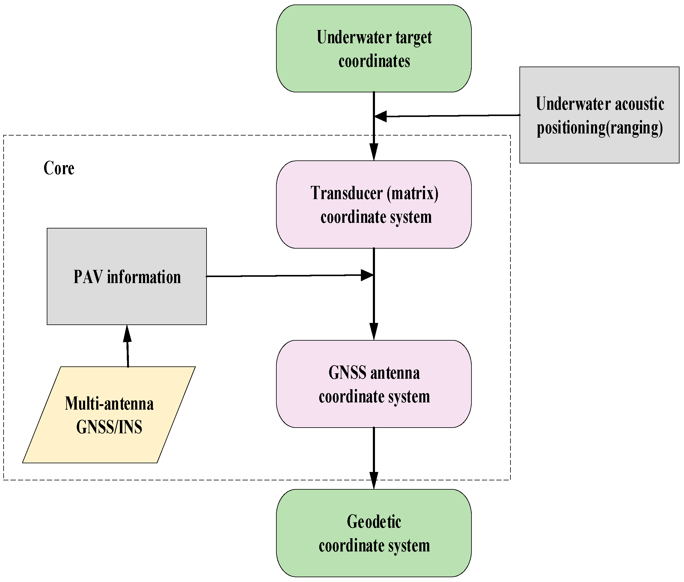
2.3. Multi-Antenna GNSS/INS Positioning Method

Through the discussion in Section 2.2, we have reached a consensus in theory; that is, due to the influence of ocean dynamic effect, the ship’s position and attitude measurements will be inaccurate, which will greatly affect the accuracy of underwater acoustic positioning results.

At present, in the special case of the remote sea, the PAV information of the survey ship is generally obtained through the output of GNSS and INS sensors. PPP technology can provide centimeter-level position and velocity information for users in this special case, and the dual-antenna RTK/PPP receiver of the commercial product ‘Vector VS1000’ can measure the attitude accuracy of 0.01° RMS and supports antenna separations up of 10 m. In particular, it is pointed out that the influence of multi-path error is very significant when GNSS alone is used for positioning at sea, which also affects the positioning accuracy to a certain extent. INS can observe the triaxial acceleration and triaxial angular velocity of the carrier with high sampling rate, which has the characteristics of a high sampling rate and is not affected by the environment. However, as the observation time increases, the measurement errors of the individual INS gradually accumulate. If the high precision of the INS is required, for example, the zero-bias error of the gyroscope reaches 0.01°/h, then the price of the sensor would be very expensive.

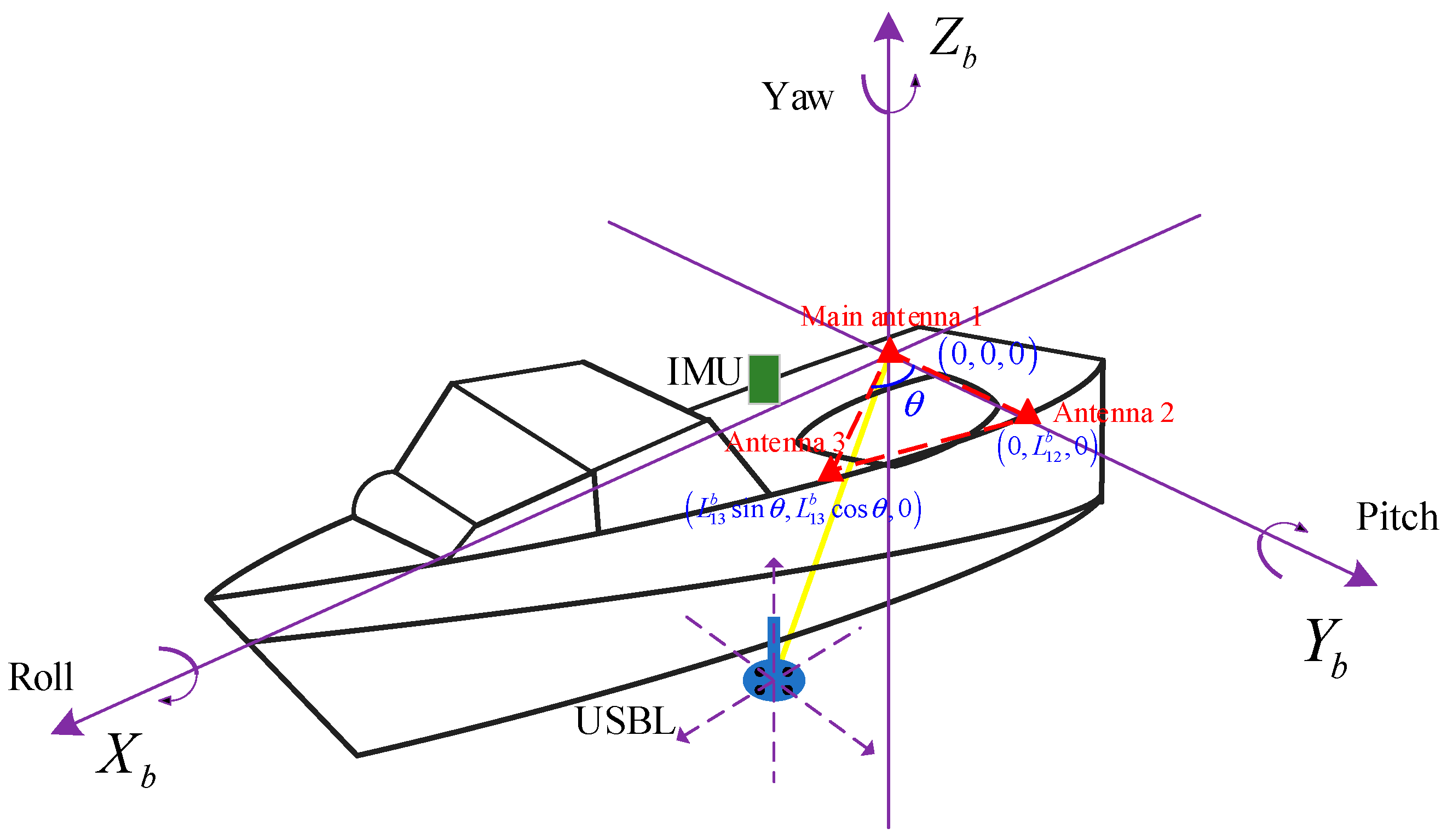
2.3.1. Multi-Antenna Attitude Measurement Method

The relationship between the position vector of the same baseline in the carrier coordinate system and the navigation coordinate system reflects the relationship of the rotation transformation between them. Using this relationship, the attitude information of the carrier can be obtained. The baseline vector of the antenna in the carrier coordinate system can be obtained through installation and calibration experiments in advance; that is, the baseline vector in the carrier coordinate system is considered to be known. Therefore, how to calculate the baseline vector in the navigation coordinate system is the focus of attitude calculation research [19].

In the GNSS attitude measurement operation, multiple GNSS receivers are required to form a small baseline attitude measurement network, and the attitude measurement based on the baseline method only requires two baselines formed by three antennas. Figure 3 shows the three-antenna installation diagram. Assuming that the main antenna coordinate is the origin of the carrier coordinate system, the coordinates of antenna 2 and 3 are ${\mathit{l}}_{12}^b=(0,L_{12}^b,0)$ and ${\mathit{l}}_{13}^b=(L_{13}^b\sin \theta ,L_{13}^b\cos \theta ,0)$, respectively; and ${\mathit{l}}_{13}^n$ are baseline vectors in the navigation coordinate system. The relationship between the two baseline vectors in the carrier coordinate system and navigation coordinate system is:

$$\left[\begin{array}{c}{\mathit{l}}_{12}^n\\ {\mathit{l}}_{13}^n\end{array}\right]={\mathit{C}}_b^n\left[\begin{array}{c}{\mathit{l}}_{12}^b\\ {\mathit{l}}_{13}^b\end{array}\right]$$

(19)

Combined with the knowledge of attitude rotation matrix, the heading angle is:

$$\psi =\arctan \left(\frac{x_{12}^n}{y_{12}^n}\right)$$

(20)

Pitch angle is:

$$\theta =\arctan \left(\frac{z_{12}^n}{\sqrt{{\left(x_{12}^n\right)}^2+{\left(y_{12}^n\right)}^2}}\right)$$

(21)

Rolling angle is:

$$\varphi =-\arctan \left(\frac{-x_{13}^n\sin \theta \sin \psi -y_{13}^n\sin \theta \cos \psi +z_{13}^n\cos \theta }{x_{13}^n\cos \psi -y_{13}^n\sin \psi }\right)$$

(22)

In fact, especially in the marine application, to ensure the safety of data quality and the reliability of results, the number of GNSS antennas will be more than three. Then there are redundant observations, the attitude angles can be regarded as unknowns, and its optimal estimated value can be obtained by the least square iteration method.

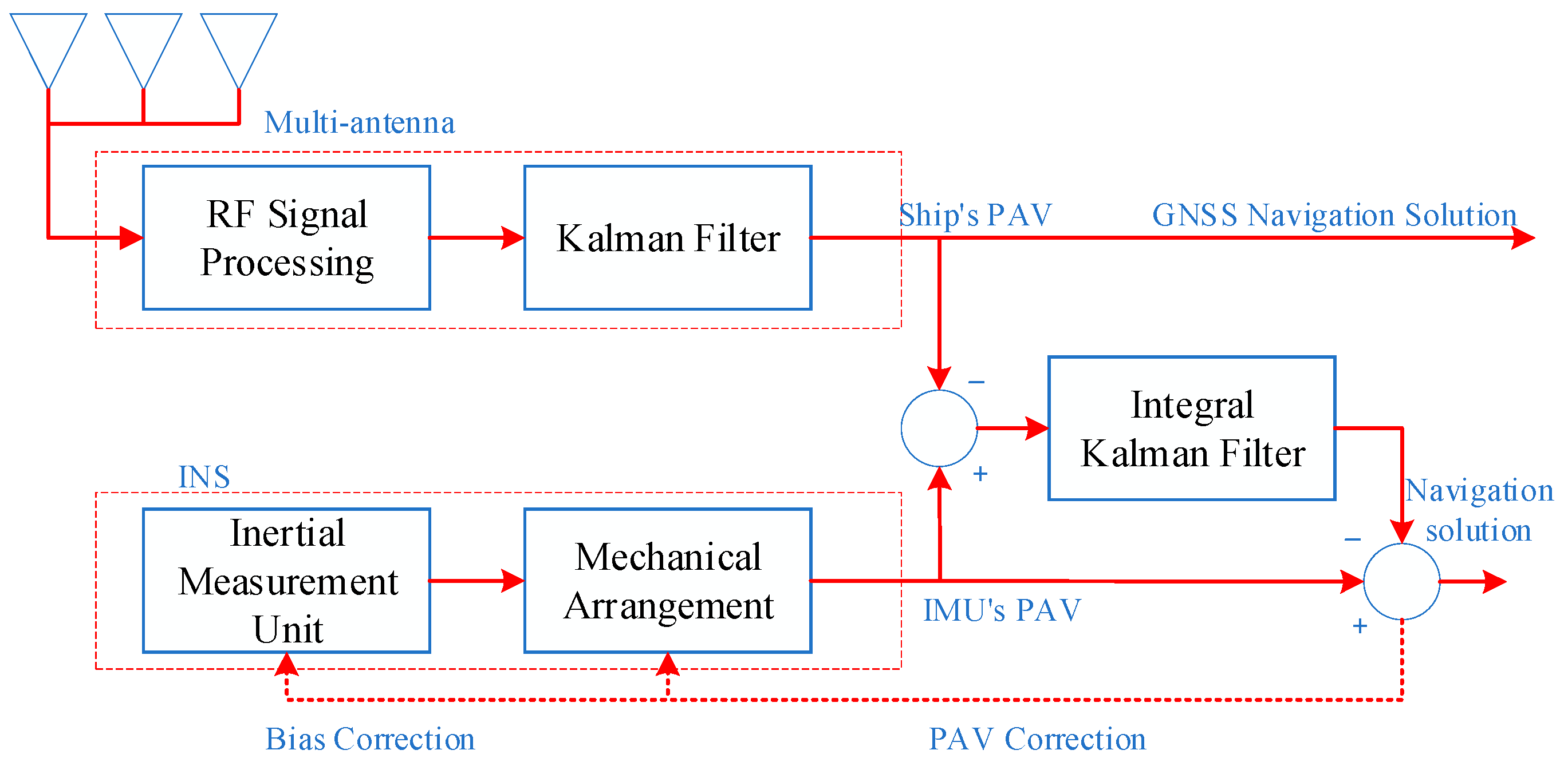
2.3.2. Multi-Antenna GNSS/INS Loose Combination Algorithm

The main idea of the multi-antenna GNSS/INS loose combination algorithm is given. First, we calculate the PAV information in the multi-antenna GNSS system and the INS system, respectively [20]. Then we use the difference between the results as the input value of the linear Kalman filter (KF) and perform parameter estimation, which is a closed estimation method, as shown in Figure 4. The ship’s sailing speed is relatively slow and linear KF can be used to deal with this problem. It should be noted that the fast and accurate ambiguity fix is also important for solving the multi-antenna attitude measurement problem, which is also one of the two main tasks that a PPP-RTK needs to accomplish [21,22].

We can construct the continuity dynamics equation of the multi-antenna GNSS/INS loose combination, which can be expressed as:

$$\dot{\mathit{X}}=F\mathit{X}+G{W}^b$$

(23)

where $\mathit{X}={\left[\begin{array}{ccccc}{\mathit{\varphi }}^{\mathrm{T}}& {(\delta v^n)}^{\mathrm{T}}& {(\delta p)}^{\mathrm{T}}& {({\epsilon }^b)}^{\mathrm{T}}& {({\mathit{\nabla }}^b)}^T\end{array}\right]}^T$ and represents misalignment error, velocity error, position error, gyroscope drift, and accelerometer bias. After discretizing the above equation, we get the equation:

$${\mathit{X}}_k={\Phi }_{k,k-1}{\mathit{X}}_{k-1}+G_k{W}_k{}^{}$$

(24)

where ${\Phi }_{k,k-1}$ is the state transition matrix, $G_k$ is the state noise allocation matrix, $W_k{}^{}$ is the state noise, and its size generally depends on the performance parameters of the IMU.

$${\Phi }_{k,k-1}\approx \exp \left(F_k\Delta t\right)=I+F_k\Delta t+\frac{1}{2}{F}_k^2\Delta t^2+\cdots$$

(25)

where $\exp (•)$ is expressed as the Taylor expansion formula.

The attitude angle error is the difference between the attitude angle estimated by the SINS system in real time and the real angle, expressed as:

$$\left[\begin{array}{c}\delta \varphi \\ \delta \theta \\ \delta \psi \end{array}\right]=\left[\begin{array}{c}{\varphi }^{\prime }-\varphi \\ {\theta }^{\prime }-\theta \\ {\psi }^{\prime }-\psi \end{array}\right]$$

(26)

where $\begin{array}{ccc}{\varphi }^{\prime }& {\theta }^{\prime }& {\psi }^{\prime }\end{array}$ are the attitude angles calculated by the strapdown inertial navigation system, and $\begin{array}{ccc}\varphi & \theta & \psi \end{array}$ are the true attitude angles. In the multi-antenna GNSS/INS integrated navigation system, the attitude information measured by GNSS is used as the real attitude angle.

The attitude angle error and the platform misalignment angle are both tiny quantities, and the second-order tiny quantities are directly ignored in the calculation process. At this time, the mathematical relationship between the attitude angle error and the platform misalignment angle error is as follows:

$$\left[\begin{array}{c}\delta \varphi \\ \delta \theta \\ \delta \psi \end{array}\right]=\frac{1}{\cos \varphi }\left[\begin{array}{ccc}-\cos \psi \cos \varphi & -\cos \varphi \sin \psi & 0\\ \sin \psi & -\cos \psi & 0\\ -\sin \varphi \sin \psi & \sin \varphi \cos \psi & -\cos \varphi \end{array}\right]·\left[\begin{array}{c}{\varphi }_E\\ {\varphi }_N\\ {\varphi }_U\end{array}\right]+v$$

(27)

where $v$ is the attitude error of multi-antenna GNSS measurement. The observation equation for velocity and position are expressed as:

$$\delta v={\tilde{v}}_{GNSS}^n-{\widehat{v}}_{GNSS}^n$$

(28)

where ${\tilde{v}}_{GNSS}^n$ is the speed of the antenna phase center calculated by INS under the local navigation system and ${\widehat{v}}_{GNSS}^n$ is the true value of GNSS antenna speed under local navigation system.

$$\delta r={\tilde{r}}_{GNSS}^n-{\widehat{r}}_{GNSS}^n$$

(29)

where ${\tilde{r}}_{GNSS}^n$ is the position of the antenna phase center calculated by INS under the local navigation system and ${\widehat{r}}_{GNSS}^n$ is the true value of GNSS antenna phase center under local navigation system.

Based on the above discussion, the GNSS/INS loose combination observation equation is established:

$$Z=\left[\begin{array}{c}{\tilde{a}}_{\mathrm{INS}}^n-{\tilde{a}}_{\mathrm{GNSS}}^n\\ {\tilde{v}}_{\mathrm{INS}}^n-{\tilde{v}}_{\mathrm{GNSS}}^n\\ {\tilde{p}}_{\mathrm{INS}}-{\tilde{p}}_{\mathrm{GNSS}}\end{array}\right]=H\mathit{X}+V$$

(30)

where $V={\left[\begin{array}{ccc}{V}_a& V_v& V_p\end{array}\right]}^T$ is the measurement noise,

$$H=\left[\begin{array}{cc}\begin{array}{cccc}{H}_{aa}& & 0_{3\times 12}& \\ -(w_{in}^n)(l_{GNSS}^n\times )-(C_b^n(l_{GNSS}^n\times w_{ib}^b))\times & I_{3\times 3}& 0_{3\times 3}& C_b^n(l_{GNSS}^b\times )\\ C_b^n(l_{GNSS}^b\times )& 0_{3\times 3}& I_{3\times 3}& 0_{3\times 6}\end{array}& 0_{3\times 3}\end{array}\right]$$

(31)

After the multi-antenna GNSS/INS loose combination model is established, we can accurately calculate the PAV information of the survey ship and reduce the influence of related errors on the positioning. Next, we will verify the influence of attitude error on the USBL positioning through experiments and test the attitude measurement effect of this model through a set of experiments.

3. Results

3.1. Influence of Attitude Angle Error on USBL

To analyze the influence of attitude error on underwater positioning, we adopted a set of USBL experiments conducted in Qingdao, China in December 2017. In this experiment, we selected the USBL array with the model “HEUUSBL6000”, and its array element spacing was 0.26 m. We chose “Applanix-POSMV 320” as the attitude sensor, and its data output frequency was up to 200 HZ. In addition, “RTK-HiPer IIG” and sound velocity profile (SVP) were installed on the surveying ship. After the relevant sensors were installed and calibrated, the navigation track was a circle with a radius of about 200 m. The experiment lasted about an hour and was completed at 6 pm. The experimental data includes GPS time, time delay measured by USBL, ship’s longitude, latitude, and elevation, ship’s, roll, pitch, and yaw, XYZ coordinates of the array, and SVP.

A total of four groups of SVP were measured in the experiment. Due to the influence of sea conditions, the sound velocity measurement data is unstable. We chose one group of relatively satisfactory SVP to use. The positioning experiment was conducted between 5 pm and 6 pm, and the measurement of SVP occurred half an hour to one hour before the beginning of the experiment. The change of the SVP in the observed sea area is shown in Figure 5. The vertical axis is the depth value (unit: m), the upper horizontal axis is the temperature (unit: degrees Celsius), and the lower horizontal axis represents the sound velocity (unit: m/s). It can be seen from Figure 5 that there is an obvious jump in the sound velocity in the same period, and it is related to the water temperature. Affected by the sea breeze within 5 m of the surface layer, the temperature is low and the sound velocity is slow, about 1447 m/s; the water temperature below 7.5 m of the surface layer gradually rises, and the sound velocity is stable at a higher position, about 1455 m/s. There is a sonic jump of about 2.5 m between 5~10 m on the surface, and the sound velocity increases rapidly. The cause of this phenomenon may be the problem of the SVP, or it may be that the ship’s disturbance to the water body is greater than the natural disturbance, which needs to be further determined.

The attitude information of the measuring ship over time can be obtained through POSMV as shown in Figure 6.

From the analysis of Figure 6, it can be seen that the roll angle of the measuring ship is between $\left(-1^{\mathrm{o}}\sim -5^{\mathrm{o}}\right)$, the pitch angle is between $\left(2^{\mathrm{o}}\sim 5^{\mathrm{o}}\right)$, and the reason for the large variation range of the heading angle is that the measuring ship is sailing in a circle.

To provide real-time RTK positioning services, we set up a GNSS reference station on Lingshan Island, and recorded and saved the raw GNSS observation data for post-processing and analysis. Post-processing using the software POS PAC, the RMS in the horizontal direction remained within 2 cm, and the results in the vertical direction were slightly less stable, but their RMS remained within 4 cm.

The positioning of the beacon is realized by the USBL algorithm, and the position of the target is integrated with the trajectory of the ship. To make it easier for readers to understand this Figure 7a, we have simplified the horizontal and vertical coordinates; that is, both X and Y have their mean values subtracted. The figure shows the corresponding results. To see the positioning results more clearly, we make a separate picture (b) of the USBL positioning results.

In Figure 7b, the red triangle Δ indicates that all the positioning results are averaged. From the results, the mean of the positioning results is almost at the origin.

Since we do not know the true value, we take the result of the experiment as the true value. To verify the influence of attitude error, we can artificially add some systematic random errors to the attitude information measured by POSMV. Using the data with the attitude observation error to perform the USBL calculation, and comparing the results with the results without the error, we can clearly see the influence of the attitude error on the positioning, thus verifying our previous discussion.

According to practical experience, we add a set of random errors to the pitch angle and roll angle respectively. We generate a set of random numbers in the range [−1, 1], and then multiply this set of random numbers by 0.1. for the heading angle, except that the random number we add to the heading angle is not multiplied by 0.1.

So, we obtained a new positioning result and compared the results of the two tests before and after as shown in Figure 8.

In Figure 8, the blue points represent the positioning results obtained when the attitude error is not included, and the red points represent the positioning results obtained after the error is added. From the results, the obvious red points are more divergent than the blue ones; the fact that the edge points are basically red further illustrates this situation; that is, the positioning results with attitude errors are worse.

We subtract the results from the two experiments to get Figure 9, where red represents the difference in the X direction, and blue represents the Y direction. Their difference bounces around 0 and ranges between [−5, 5].

Through the above experiments, we can draw a conclusion that the existence of attitude error will significantly reduce the accuracy of underwater positioning, resulting in inaccurate positioning results. Therefore, to perform high-precision positioning at sea, the attitude information must be accurately measured. Next, we will demonstrate through experiments that the multi-antenna GNSS/INS combination algorithm can achieve accurate attitude measurement.

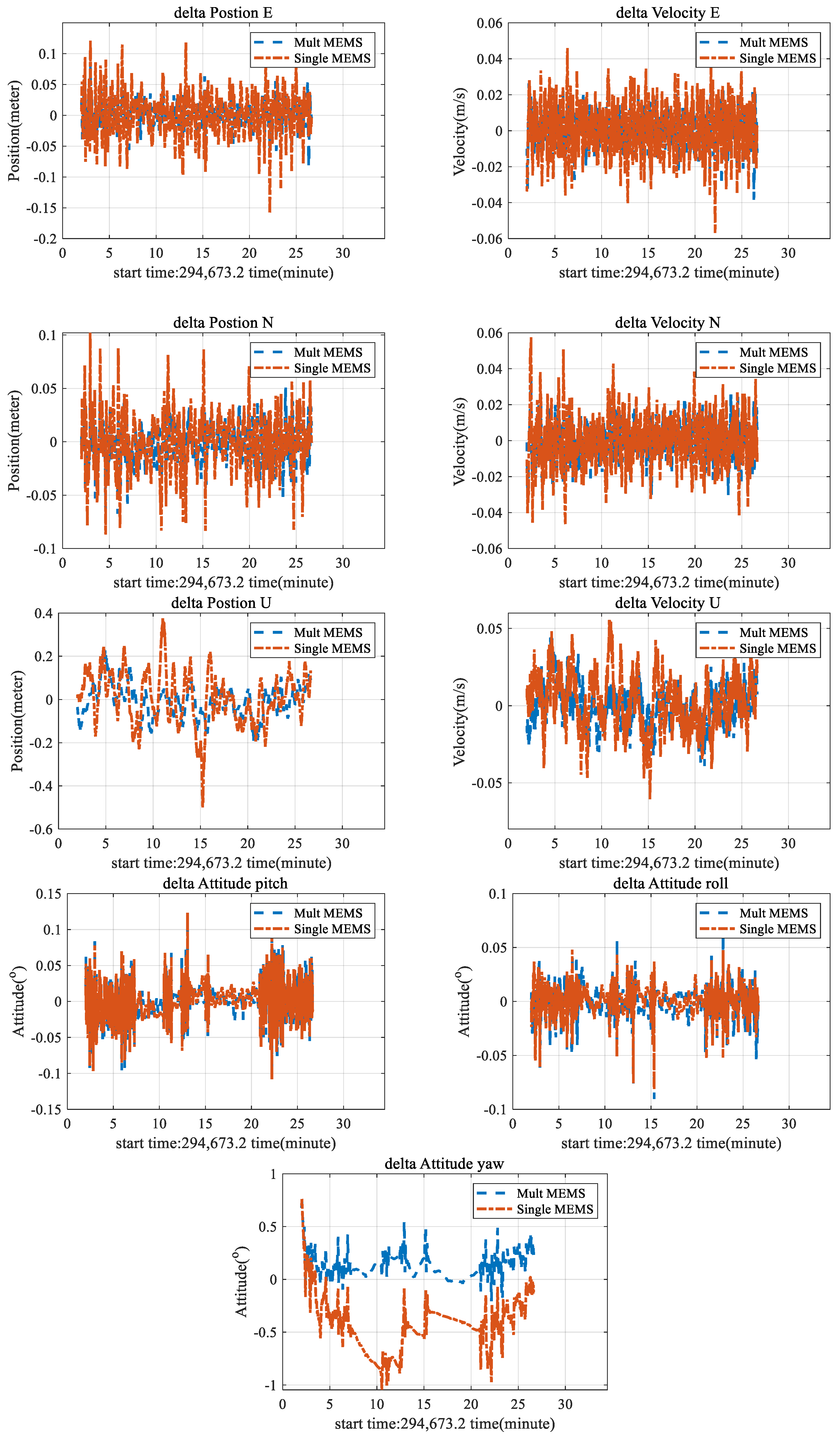
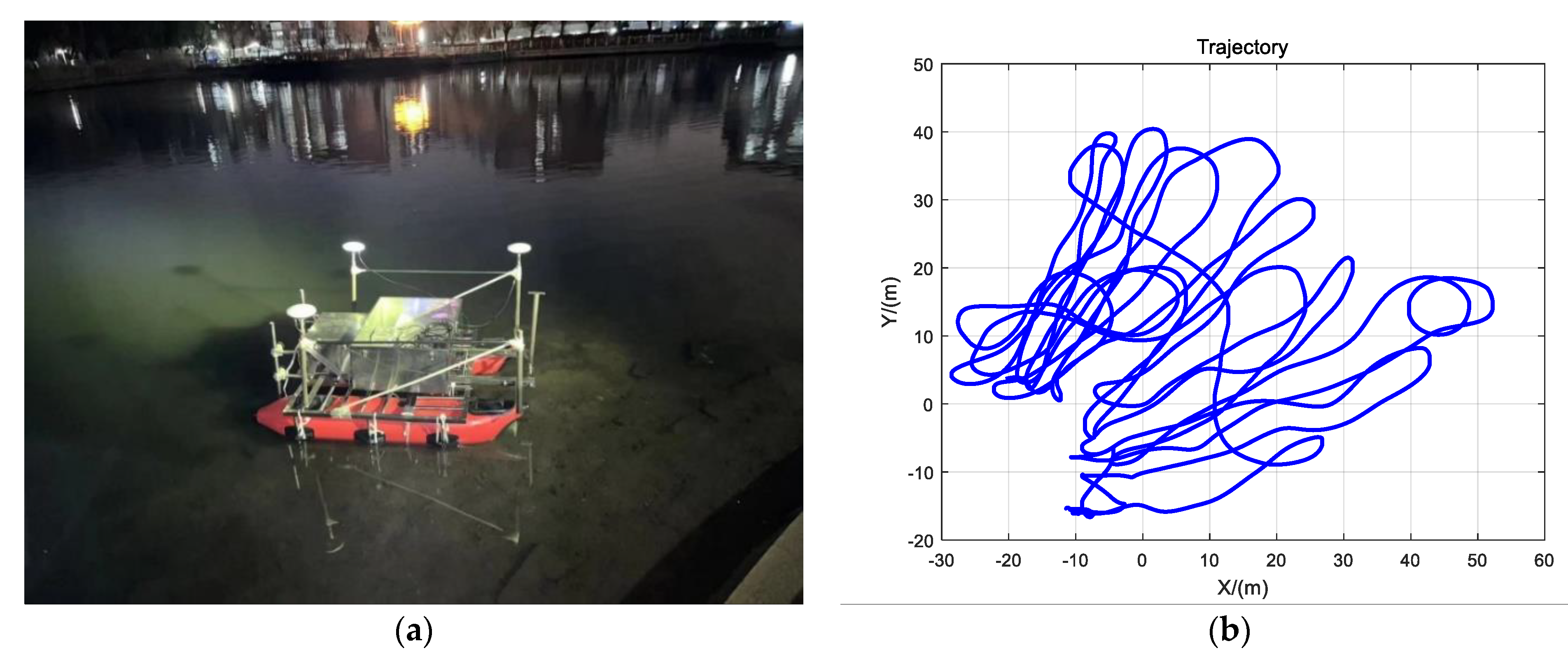
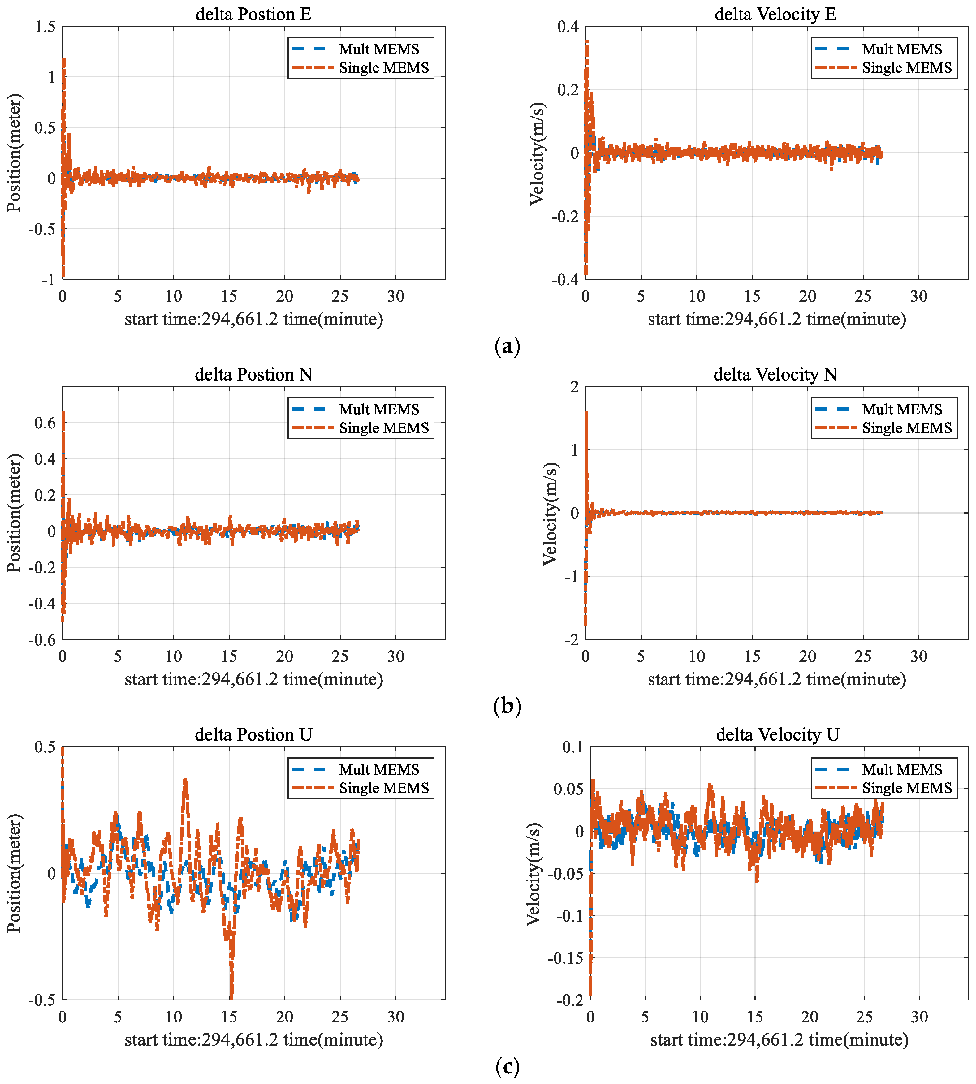
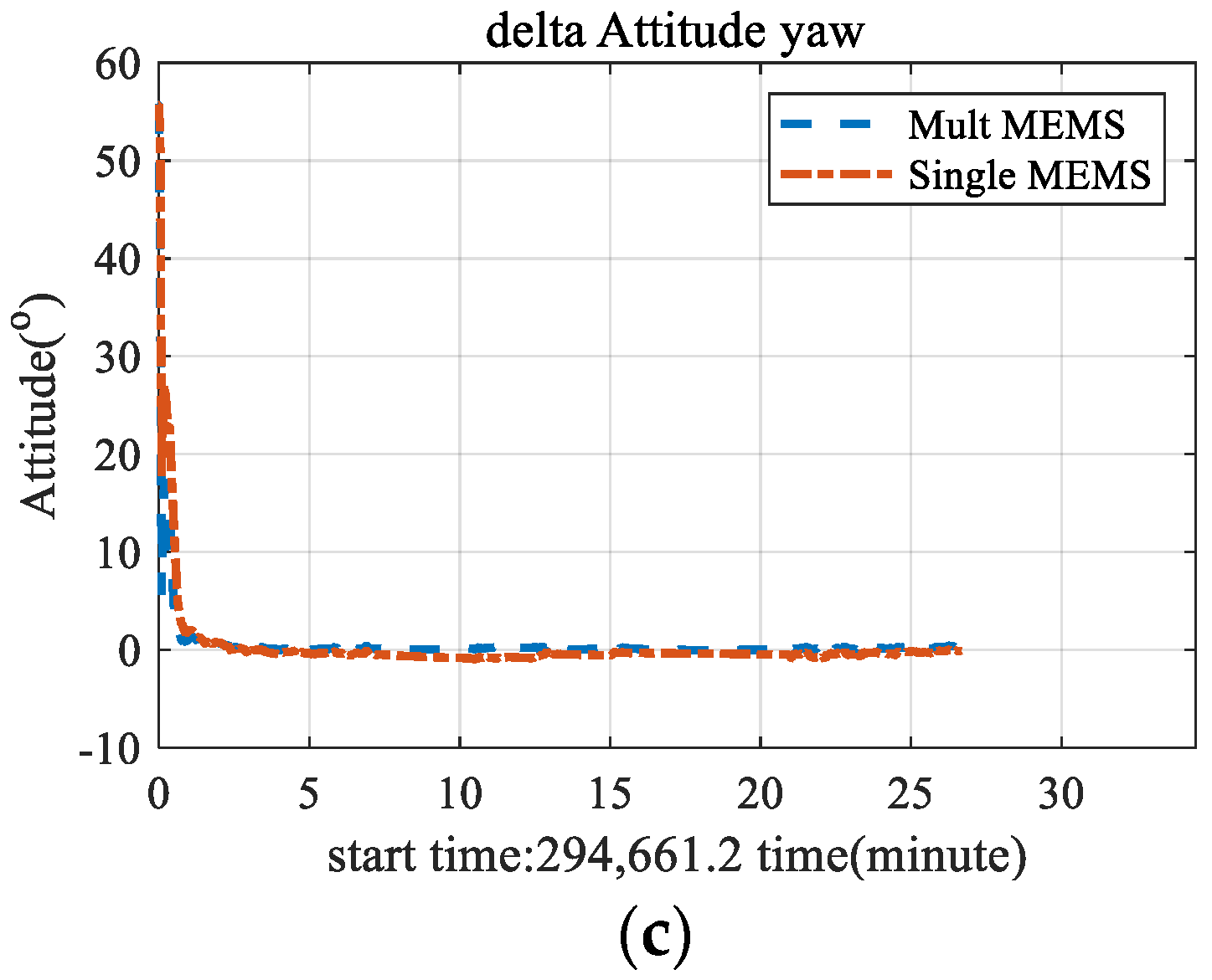
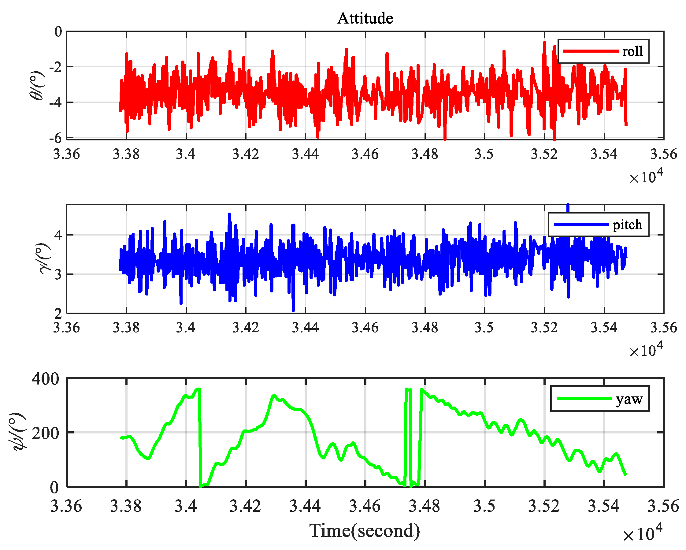
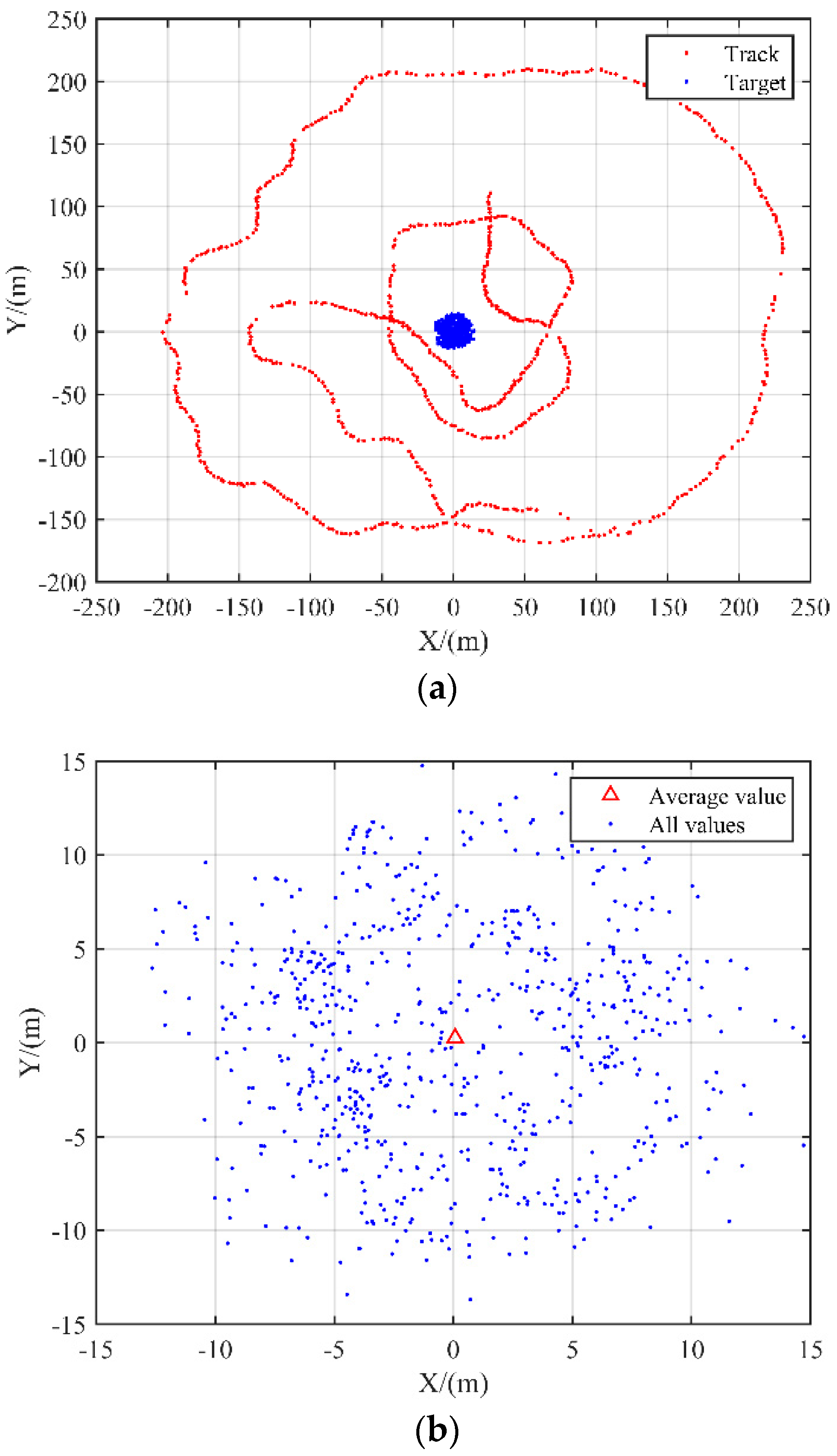
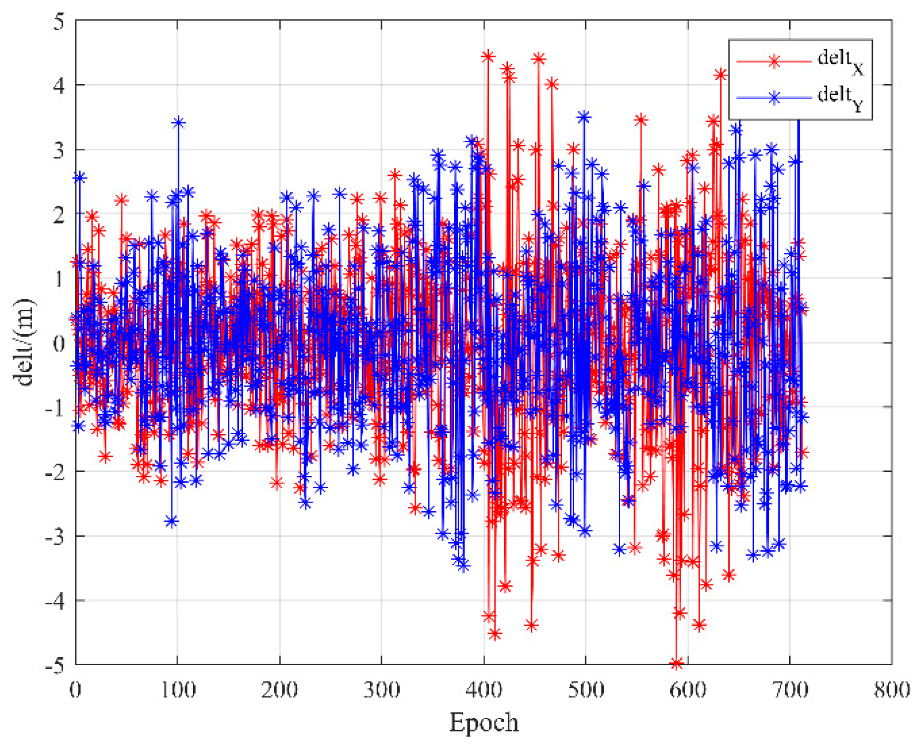
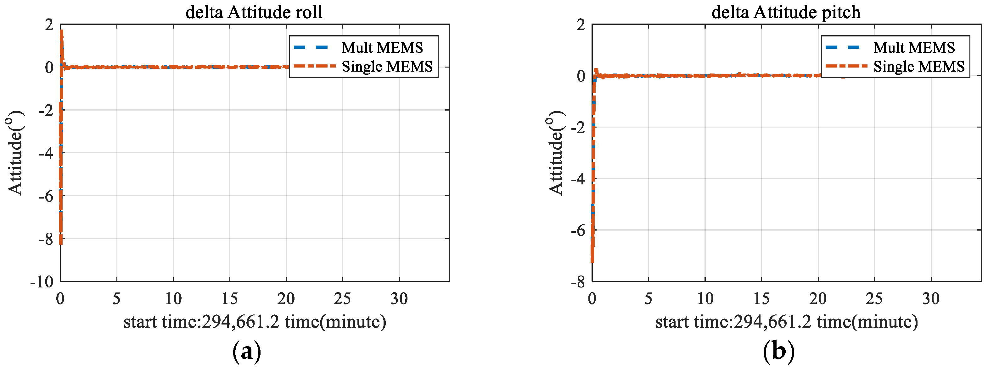
3.2. Multi-Antenna GNSS/INS Attitude Measurement Test

The experiment was conducted in a lake at Shandong University of Science and Technology in Qingdao, China. The RTK mode is used to locate a small, unmanned ship and the reference station is placed on the roof of a teaching building with a wide view. Three GNSS antennas and HG-4930 MEMS sensors are installed on the ship. For comparative tests, the LCI’s fiber-optic IMU was also installed on it. The HG-4930 MEMS sensors, gyro range is −325°/s to +325°/s. Gyro stability is up to 0.3°/h. Accelerometer random walk is 100 ug/sqrt (Hz). Sampling frequency is 100 HZ. The integrated navigation system is independently developed by our team. Positioning accuracy is 5 cm. Velocity accuracy is 5 cm/s. Attitude measurement is 1° (under the constraints of multiple antennas, the attitude accuracy can reach 0.05°). In addition, multi-antennas are installed on the iron frame by fixed connection, and the distance relationship between them is accurately measured by the total station.

The unmanned ship stayed stationary at the shore for a period of time to reserve data for the static initial alignment. At the beginning of the experiment, the unmanned ship moved around a graphic trajectory of 8. Then the unmanned ship dynamically ran around the test site. Restricted by the size of the lake, the unmanned ship could not travel in a straight line for a long time, so the main navigation trajectory is an arc. Figure 10 shows the navigation trajectory of the ship and, to make the figure easier to read, we subtracted their own mean from both X and Y. The results are obtained by Inertial Explorer 8.7.

Both GNSS and INS can output position, velocity, and attitude information. A loose combination model based on multi-antenna GNSS/INS is constructed according to the discussion in Section 2.3.2. The state parameters are obtained by the ARKF (adaptive robust Kalman filtering) solution considering the motion characteristics of the offshore platform, and the result of the LCI output was solved by Inertial Explorer 8.7 as the true value. In particular, ARKF uses the prediction residual to improve the weight matrix of the prediction state vector to make an optimal estimate for the system calculation. Compare the results of single/multi-antenna GNSS/INS loose combination algorithm with the true value, the variation relationship of the deviation value with time can be obtained by subtraction, as shown in Figure 11 and Figure 12.

In particular, the attitude error of the three-axis is relatively large at the beginning because the baseline vector value used for the three-antenna attitude at this time is a floating-point solution, which has a great influence on the solution result. This also results in the attitude results of the three antennas not being optimal at the beginning. When the ambiguity is fixed, the accuracy of the attitude solution results quickly converges, and the accuracy is improved significantly.

To make the results in Figure 11 and Figure 12 clearer, we removed the pre-convergence results so that the values are shown around 0. We put the new figures in Appendix A, from Figure A1, which can more clearly show the experimental results and verify the previous conclusions.

4. Discussion

According to Figure 11 and Figure 12,

Table 1. Comparison of position, velocity, and attitude accuracy between single-antenna model and multi-antenna model.

		Multi Antenna	Single Antenna
	E	0.0423	0.0377
Position (m)	N	0.0524	0.0558
	U	0.1225	0.1084
	E	0.0746	0.0709
Velocity (m/s)	N	0.0243	0.0238
	U	0.0195	0.0182
	Roll	0.2705	0.3008
Attitude (°)	Pitch	0.2833	0.3100
	Yaw	2.5639	3.6273

and Appendix A, from the analysis of E and N directions, compared with the single-antenna GNSS/INS loose combination algorithm, the multi-antenna GNSS/INS loose combination algorithm has no obvious advantages. From the analysis of the U direction, the deviation value under the multi-antenna model is smaller. For the attitude information analysis, the multi-antenna mode improves the heading angle accuracy by about 29.3% compared to the single-antenna mode. It can be seen that the measurement accuracy of the multi-antenna model in the heading angle direction is greatly improved; the measurement accuracy of pitch and roll angles is slightly improved, mainly because of the small changes in pitch and roll angles during the test.

If the ship has a long-term linear motion or a stationary state, and is under the combined actions of sea surface swells, there will be a situation of sideslip and drift; if the ship is traveling slowly or shaking violently, the attitude calculation will not be completed. The multi-antenna GNSS/INS loose combination algorithm has unique advantages in solving this problem.

5. Conclusions

The traditional single-antenna GNSS/INS measurement mode may have good results in vehicle positioning on land, but it is not suitable for marine environments. From the experiment we can learn that the roll angle of the measuring ship is between $\left(-1^{\mathrm{o}}\sim -5^{\mathrm{o}}\right)$, the pitch angle is between $\left(2^{\mathrm{o}}\sim 5^{\mathrm{o}}\right)$, and the range of change in heading angle will be larger. Experiments show that we add small error disturbances to the attitude angles, resulting in more than 5 m of deviation by USBL positioning. Figure 9 shows that the deviation in the X and Y directions is between [−5, 5]. Especially if the ship is traveling slowly or shaking violently, the attitude calculation will not be challenging, and the traditional single-antenna GNSS/INS measurement mode is not suitable.

We get better PAV results with the multi-antenna GNSS/INS loose combination algorithm. Compare the results of the single/multi-antenna GNSS/INS loose combination algorithm with the true value, and the variation relationship of the deviation value with time can be obtained by subtraction, as shown in Figure 11 and Figure 12. Combined with the results in Table 1, we find that for the E and N directions, the output results of the multi-antenna model are better, but due to the impact of the test environment, its significance is slightly poor; for the attitude information analysis, the multi-antenna mode improves the heading angle accuracy by about 29.3% compared to the single-antenna mode.

To sum up, the multi-antenna GNSS/INS loose combination algorithm can output higher-precision PAV information. In particular, the attitude measurement accuracy in the three DoF are improved by 10.1% (roll), 8.6% (pitch), and 29.3% (yaw), thereby reducing the influence of system errors on USBL positioning results and improving the reliability and robustness of underwater acoustic positioning.

References

1. Yang, Y.; Liu, Y.; Sun, D.; Xu, T.; Xue, S.; Han, Y.; Zeng, A. Seafloor geodetic network establishment and key technologies. Sci. China Earth Sci. 2020, 63, 1188–1198. [Google Scholar] [CrossRef]
2. Yang, Y. Concepts of comprehensive PNT and Related Key Technologies. Acta Geod. Cartogr. Sin. 2016, 45, 505–510. [Google Scholar] [CrossRef] [Green Version]
3. Liu, Y.; Lu, X.; Xue, S.; Wang, S. A new underwater positioning model based on average sound speed. J. Navig. 2021, 74, 1009–1025. [Google Scholar] [CrossRef]
4. Fujita, M.; Ishikawa, T.; Mochizuki, M.; Sato, M.; Toyama, S.; Katayama, M.; Kawai, K.; Matsumoto, Y.; Yabuki, T.; Asada, A.; et al. GPS/Acoustic seafloor geodetic observation: Method of data analysis and its application. Earth Planet Space 2006, 58, 265–275. [Google Scholar] [CrossRef] [Green Version]
5. Zhao, S.; Wang, Z.; He, K.; Ding, N. Investigation on Underwater Positioning Stochastic Model Based on Acoustic Ray Incidence Angle. Appl. Ocean Res. 2018, 77, 69–77. [Google Scholar] [CrossRef]
6. Liu, Y.; Xue, S.; Qu, G.; Lu, X.; Qi, K. Influence of the ray elevation angle on seafloor positioning precision in the context of acoustic ray tracing algorithm. Appl. Ocean Res. 2020, 105, 102403. [Google Scholar] [CrossRef]
7. Kussat, N.H.; Chadwell, C.D.; Zimmerman, R. Absolute positioning of an autonomous underwater vehicle using GPS and acoustic measurements. IEEE J. Ocean. Eng. 2005, 30, 153–164. [Google Scholar] [CrossRef]
8. Jin, S.; Liu, G.; Sun, W.; Bian, G.; Cui, Y. The Research on Depth Reduction Model of Multibeam Echosounding Considering Ship Attitude and Sound Ray Bending. Hydrogr. Surv. Charting 2019, 39, 5. [Google Scholar] [CrossRef]
9. Fund, F.; Perosanz, F.; Testut, L.; Loyer, S. An Integer Precise Point Positioning technique for sea surface observations using a GPS buoy. Adv. Space Res. 2013, 51, 1311–1322. [Google Scholar] [CrossRef]
10. Gao, Z.; Zhang, H.; Ge, M.; Niu, X.; Shen, W.; Wickert, J.; Schuuh, H. Tightly coupled integration of multi-GNSS PPP and MEMS inertial measurement unit data. GPS Solut. 2017, 21, 377–391. [Google Scholar] [CrossRef]
11. Eling, C.; Zeimetz, P.; Kuhlmann, H. Development of an instantaneous GNSS/MEMS attitude determination system. GPS Solut. 2013, 17, 129–138. [Google Scholar] [CrossRef]
12. Chai, Y.; Hu, F.; Zhong, S. Analysis on Results of Multi-antenna GNSS/INS. In Proceedings of the 12th China Satellite Navigation Annual Conference—S09, User Terminal Technology, Nanchang, China, 26–28 May 2021; pp. 146–150. [Google Scholar] [CrossRef]
13. Yang, W.; Xue, S.; Liu, Y. P-Order Secant Method for Rapidly Solving the Ray Inverse Problem of Underwater Acoustic Positioning. Mar. Geod. 2021, 1–13. [Google Scholar] [CrossRef]
14. Chen, G.; Liu, Y.; Liu, Y.; Liu, J. Improving GNSS-acoustic positioning by optimizing the ship’s track lines and observation combinations. J. Geod. 2020, 94, 61. [Google Scholar] [CrossRef]
15. Zheng, C. Application of USBL Positioning Technology on Underwater Submersible InterCall; Harbin Engineering University: Harbin, China, 2008. [Google Scholar]
16. Zheng, C.; Li, Z.; Sun, D. Study on the calibration method of USBL system based on ray tracing. Oceans IEEE 2013, 1–4. [Google Scholar] [CrossRef]
17. Wu, Y. Study on Theory and Method of Precise LBL Positioning and Development of Positioning Software System; Wuhan University: Wuhan, China, 2013. [Google Scholar]
18. Zhao, J.; Liu, J.; Zhang, H. The Analysis of Vessel Attitude and the Effect for Multibeam Echo Sounding. Geomat. Inf. Sci. Wuhan Univ. 2001, 26, 144–149. [Google Scholar] [CrossRef]
19. Zhao, Y.; Zou, J.; Zhang, P.; Guo, J.; Wang, X.; Huang, G. An Optimization Method of Ambiguity Function Based on Multi-Antenna Constrained and Application in Vehicle Attitude Determination. Micromachines 2022, 13, 64. [Google Scholar] [CrossRef] [PubMed]
20. Cai, X.; Hsu, H.; Chai, H.; Ding, L.; Wang, Y. Multi-antenna GNSS and INS Integrated Position and Attitude Determination without Base Station for Land Vehicles. J. Navig. 2019, 72, 342–358. [Google Scholar] [CrossRef]
21. Zhang, B.; Hou, P.; Zha, J.; Liu, T. Integer-estimable FDMA model as an enabler of GLONASS PPP-RTK. J. Geod. 2019, 95, 91. [Google Scholar] [CrossRef]
22. Zhang, B.; Chen, Y.; Yuan, Y. PPP-RTK based on undifferenced and uncombined observations: Theoretical and practical aspects. J. Geod. 2019, 93, 1011–1024. [Google Scholar] [CrossRef]
Figure 1. The positioning geometry principle with ultra-short baseline.
Remotesensing 14 03878 g001
Figure 2. The coordinate transformation process.
Remotesensing 14 03878 g002
Figure 3. Three-antenna installation diagram.
Remotesensing 14 03878 g003
Figure 4. Multi-antenna GNSS/INS loose combination algorithm model.
Remotesensing 14 03878 g004
Figure 5. SVP (depth, sound velocity, and temperature).
Remotesensing 14 03878 g005
Figure 6. Changes of the three attitude angles.
Remotesensing 14 03878 g006
Figure 7. (a) Ship’s trajectory and USBL positioning results; (b) enlarged view of USBL positioning results and the mean value of all the results.
Remotesensing 14 03878 g007
Figure 8. Comparison of the results of the two experiments.
Remotesensing 14 03878 g008
Figure 9. Comparison of deviation values in X and Y directions.
Remotesensing 14 03878 g009
Figure 10. (a) Unmanned ship carrier platform for testing; (b) the trajectory of the unmanned ship.
Remotesensing 14 03878 g010
Figure 11. Deviation of position and velocity. (a) Position deviation and velocity deviation in the E direction. (b) Position deviation and velocity deviation in the N direction. (c) Position deviation and velocity deviation in the U direction.
Remotesensing 14 03878 g011
Figure 12. Comparison of attitude deviation under two models. (a) Deviation of roll. (b) Deviation of pitch. (c) Deviation of yaw.
Remotesensing 14 03878 g012aRemotesensing 14 03878 g012b