Monitoring Heat Extremes across Central Europe Using Land Surface Temperature Data Records from SEVIRI/MSG

Abstract

The frequency and intensity of extreme hot events have increased worldwide, particularly over the past couple of decades. Europe has been affected by unprecedented mega heatwaves, namely the events that struck Western Europe in 2003 and Eastern Europe in 2010. The year 2018 was also reported as an unusually hot year, with record-breaking temperatures in many parts of Europe during spring and summer, associated with severe and unusual wildfires and significant crop losses in central and northern Europe. We show the ability of Land Surface Temperature (LST), retrieved from the Spinning Enhanced Visible and Infrared Imager (SEVIRI) onboard Meteosat Second Generation (MSG) to monitor heat extremes, using the 2018 European event as a showcase. The monitoring approach relies on monthly anomalies performed as departures from the median and the monthly number of hot days (NHD), both computed for satellite LST derived from MSG and MODIS, and for 2 m air temperature (T2m) from ERA5 reanalysis, using as threshold the 90th percentiles. Results show strong monthly LST anomalies during the spring and summer of 2018 extending over central and north Europe. Over a vast region in Central and Northern Europe, LST reached the last 15 years high record. Moreover, those outstanding warm LSTs persisted for more than four months. Results obtained using MODIS LST and ERA5 T2m show similar patterns, which, although slightly less intense, corroborate the exceptionality of the heat extremes observed over central and northern Europe during 2018. The spatial pattern of the number of monthly record high anomalies over the MSG observations period clearly depicts the regions in Northern and Central Europe affected by the complex phenomena that occurred in 2018, which resulted from the combined effect of an extreme heatwave in spring and summer with extensive dry conditions. Therefore, the results highlighted the suitability of MSG LST to evaluate and monitor heat extremes alone or combined with dry and bright conditions and prompts the potential of other climate data records from geostationary satellites to characterize these climate extremes that could become the norm in the near future over central and northern Europe.

1. Introduction

In 2018, record-breaking temperatures were observed during spring and summer simultaneously throughout the world, namely in Europe, North America, and Asia [1]. Europe experienced an outstanding warm and dry year, with late spring and summer temperatures 1 °C warmer than 1981–2010 normal values. Exceptional temperatures were observed over Scandinavia, Central Europe, the Iberian Peninsula, and the British Isles, affecting different regions during different months/weeks [2]. As a result, the 2018 summer was classified as the warmest since 1500, surpassing the previous events of 2003 and 2010, with an area affected by extreme drought far larger than the ones observed during 2003 and 2010 [2,3,4]. Summer heat and precipitation deficits both contributed, although unevenly within the affected areas, to the extreme 2018 European summer drought. In particular, the quick move from a wet spring to dry summer conditions, combined with strong temperature and radiation anomalies in the previous spring, has been pointed to as a trigger of the summer extreme drought event [4]. Therefore, land–atmosphere feedbacks play an active role in amplifying extremely high temperatures by previous and concurrent dry conditions in Northern and Central Europe [5,6] and vice versa [4].

The devastating impacts of the recent heat and dry extremes have been reported to disturb several sectors of society and natural ecosystems. During the 2003 summer period, 70,000 additional deaths were recorded in Europe, while no harvesting disturbance was observed in the months following August 2003 [7]. Conversely, the 2010 Russian heatwave had overwhelming impacts on a wide range of areas. These impacts were mainly associated with thousands of casualties, significant crop losses, millions of hectares of burnt areas, and enormous economic losses [8]. The 2018 warm temperatures and precipitation deficits align with the observed increase in intensity and frequency of extremely hot and dry events over many regions [9,10]. Between May and July 2018, 13 European countries reported heat-related impacts covering different sectors [1]. Devastating fires destroyed large areas of intact forests, not only in countries with a long tradition of wildfires, such as Portugal, Spain, and Greece but also in countries with less history of large fires, such as Sweden, Norway, Finland, and Latvia. The hot temperatures have also triggered crop loss of up to 50% in Switzerland, British Isles, Russia, and Germany and contributed to power shortages and power production decrease in France, Switzerland, and Germany. The rails bucked and the roads melted in the British Isles and the Netherlands [1,3].

Several authors have analyzed the dynamical mechanisms behind the recent heat and dry extremes using different datasets of in situ and modeled data [1,2,3,4,11,12,13,14]. An unprecedented climate extreme was reported in Northern and Eastern Europe due to a compounding of extreme conditions: a particularly dry spring and exceptionally persistent warm spring temperatures, together with an outstanding dry and hot summer [3,11]. The growing season and wheat development were constrained by the compound warm and dry conditions that led to yield and quality losses, a factor that can have severe impacts on food security [12]. According to future scenarios, the intensity and frequency of heat and dry extremes are projected to increase significantly [12,15] highlighting the need for the continuous monitoring of these extreme events, separately or compounded.

In recent years, remote sensing data records have become valuable data sources that cover large areas with high temporal resolution and are now available for extended periods (some data records have been available now for over 40 years, such as those based on observations made by the Advanced Very High-Resolution Radiometer, AVHRR). Since the early 21st century, new products to characterize surface radiation balance have been available for sensors onboard polar and geostationary satellites. Land Surface Temperature (LST) may be regarded as the radiative skin temperature of the land surface that emits IR radiance [16], as measured in the direction of the sensor. LST obtained from the Spinning Enhanced Visible and Infrared Imager (SEVIRI) onboard Meteosat Second Generation (MSG) has been generated operationally since 2005 and disseminated, in near-real time, with a temporal sampling of 15 min, by LSA-SAF (Satellite Application Facility on Land Surface Analysis) as part of the EUMETSAT (European Organization for the Exploitation of Meteorological Satellites) Ground Segment. In recent years, the generation of a long-term dataset has been envisaged, and therefore, LST obtained from SEVIRI/MSG (hereafter called MSG LST) was reprocessed with a temporal sampling of 15 min from 2004 to 2015, which warrants a highly homogeneous and consistent dataset (i.e., with no changes to the retrieval algorithm and its inputs throughout the whole period).

The validation of LST remote sensing products using in situ observations is not straightforward, given the high spatial and temporal variability of LST. The LSA-SAF LST data have gone through extensive quality assessment studies to evaluate the accuracy and precision of estimates in comparisons with reference measurements/products over a wide range of surface conditions and using well-established methodologies (e.g., [17]). On top of those, the products’ temporal stability is also checked through the analysis of changes in time of possible biases against those reference measurements/products. The validation of the MSG LST product against ground observations, following a careful assessment of the representativeness of each station at the pixel scale, suggests overall accuracies of 0.33 °C [18]. Better matches are usually found for nighttime observations, highlighting the influence of LST spatial and temporal variability and sensor view angle on satellite daytime estimates. Overall, the MSG LST dataset is consistent and meets high accuracy standards [18]. Results from the evaluation of decadal stability of the reprocessed data record of MSG LST performed using ECMWF ERA Interim skin temperature, and Modis LST Level-2 v006 MOD11_L2 and MYD11_L2 from Terra and Aqua satellites show very good results in achieving the target stability requirement of 0.4 K/decade over several places [19].

In recent years, the availability of satellite-derived datasets updated in near-real time (NRT) and covering almost two decades of information opens a window of opportunity for flexible and simple strategies for the monitoring and characterization of climate extreme events. In this context, the main objective of the present work is to show the ability to use LST from SEVIRI on MSG to monitor heat extremes, specifically by (i) assessing the consistency between LSTs derived from MSG/SEVIRI and MODIS; (ii) characterizing the monthly evolution of MSG LST over the European region during the hot 2018 year; (iii) comparing the ability of MSG LST and LST-MODIS to monitor the heat extreme event of 2018; and (iv) comparing the results using remote sensing data with more traditional methods using 2 m air temperature from ERA5 reanalysis. In this work, LST is used to evaluate the exceptional character of the 2018 heat extreme; however, due to its radiometric character, which is mainly related to the radiation budget and moisture at the surface, an integrated vision of the impact of the extreme conditions during spring and summer conditions is foreseen. Therefore, we expect to demonstrate the usefulness of remote sensing data to monitor in near-real time the evolution of heat extremes such as the ones that occurred in 2018, specifically by computing climate indices such as the number of hot days [18].

2. Materials and Methods

2.1. Data

2.1.1. MSG LST

LSA-SAF retrieves LST from cloud-screened SEVIRI/MSG measurements in the thermal infrared, with a temporal frequency of 15 min and at the original spatial resolution-geostationary grid with a 3 km sampling distance at the satellite nominal sub-satellite point at 0° longitude. The LSA-SAF uses a split-window algorithm where LST is derived from top-of-atmosphere brightness temperatures of the SEVIRI split-window channels (centered at 10.8 and 12.0 micro-m, respectively) and assuming the surface emissivity to be determined by combining SEVIRI fraction of vegetation cover (also provided by the LSA-SAF) and the land-cover classification assigned to each pixel—please see further details in [20]. The MSG LST dataset is freely available at (https://landsaf.ipma.pt/en/, accessed on 14 July 2022) for two “subset” datasets: (i) the so-called Near-Real Time (NRT) product (LSA-004), which is generated operationally and disseminated with a temporal sampling of 15 min and (ii) the so-called Climate Data Record (CDR) product (LSA-050), reprocessed in 2017 for the period between 2004 to 2015 also with a temporal sampling of 15 min, using the same algorithm version in place for the NRT product. Several validation exercises using in situ observations were performed on LST NRT and CDR products and show that the MSG LST dataset is consistent and meets high accuracy standards [18,19,20,21,22]. Ground observations are routinely used to validate LST-MSG products, considering the representativeness of each station at the pixel scale. Results from the in situ satellite comparisons show overall accuracy of 0.13 °C and a root mean square error (RMSE) of about 1.9 °C [18]. Nighttime observations usually correspond to better matches with an accuracy of 0.05 K and RMSE of 1.7 °C, while daytime MSG LST values reveal an overall accuracy of 0.34 °C and RMSE of about 2.0 °C [18]. These results show that the LST-MSG dataset is consistent and meets high accuracy requirements while highlighting the effect of LST spatial and temporal variability and of sensor view angle on the higher uncertainty of satellite daytime estimates.

2.1.2. LST-MODIS

MODIS is a passive imaging instrument flying onboard Terra and Aqua polar-orbiting satellites, acquiring information in 36 spectral bands. Both orbits are sun-synchronous, and Terra’s orbit passes from north to south across the Equator in the morning (10:30, local solar time), whereas Aqua passes south to north in the afternoon (1:30, local solar time). Terra MODIS and Aqua MODIS revisiting times are about 1 to 2 days. Although there are some well-known problems with some MODIS bands, each collection/version of their products mitigates those problems with newer calibration coefficients (e.g., [23]).

MODIS LST retrieves LST from cloud-screened MODIS-Aqua imagery. As obtained through validation field campaigns and radiance-based studies, the accuracy of MODIS LST products is generally better than 1 K [24]. Arid regions exhibit higher errors due to emissivity values and heavy dust aerosol loads. The contamination by clouds and heavy aerosols may lead to errors from 4 to 11 K [24]. The latest version of the product (used in this validation exercise) mitigates some of these deficiencies [25]. Data from the Level 3 v006 MYD11 (MODIS-Aqua) collection between 2004 and 2019 were used. These datasets are available per tile of a global sinusoidal projection in daily files, containing both daytime and nighttime data.

2.1.3. ERA5

The ERA5 reanalysis is produced by the European Centre for Medium-Range Weather Forecasts (ECMWF) within the Copernicus Climate Service (C3S) framework. ERA5 encompasses hourly data from 1979 onwards (preliminary data from 1950 onwards is already available on the Climate Data Store portal) on a 31 km resolution grid. ERA5 reanalysis builds upon the ERA Interim reanalysis, which spanned 1979 onwards on a grid of approximately 80 km spatial resolution, four times a day (00, 06, 12, and 18 UTC). ERA5 re-forecast analyses show a gain of up to one day in skill compared to ERA Interim [26].

The ERA5 2 m Air Temperature (T2m) corresponds to the air temperature at 2 m above the surface over land, sea, or inland waters. This temperature is computed by interpolating between the temperatures from Earth’s surface and the lowest model level, considering the atmospheric conditions. T2m is commonly used in climate studies, specifically to compute climate indices, such as the number of hot/cold days (NHD/NCD) [5].

2.1.4. International Geosphere–Biosphere Program (IGBP) Land-Cover Classification

The International Geosphere–Biosphere Program (IGBP) land-cover classification scheme [27] consists of 17 land-cover classes that meet the needs of IGBP core science projects and, at the same time, are compatible with the classification systems used for environmental modeling. The IGBP land-cover map is re-gridded to the same grid used to compare the MSG LST product. Due to their similar behavior in terms of LST, some IGBP classes are aggregated to simplify the analysis: evergreen/deciduous and needleleaf/broadleaf forests were classified as forests; open shrublands, woody savannas, and savannas as savannas; croplands and croplands/natural vegetation mosaics as croplands.

2.2. Methods

Remotely sensed LST estimates are highly sensitive to characteristics of the measuring instrument, specifically the spatial sampling and viewing geometries, as well as to the algorithms and auxiliary data used in the retrievals—most notably, assumptions about surface emissivity (e.g., [18]). For this reason, we first compare MSG LST to MODIS LST (MYD11) over a large spatial domain (15°W–25°E, 20°N–60°N) encompassing the Europe and North Africa regions for the reprocessing period (2004–2015). The comparison is performed for January and July (and day and night times, respectively). Only data from MODIS-Aqua are used since its day overpassing time roughly corresponds to the daily temperature maximum, which is used to compute the number of hot days. Both datasets are resampled to a 0.05° × 0.05° regular grid by averaging all valid matchups (i.e., valid pairs of MSG and MODIS LST pixels used for comparison for the same location) falling into each grid cell. A statistical analysis of the difference between MSG LST and MODIS LST is performed for the main IGBP land-cover types over the European region. Figure 1 shows the median differences between MSG LST and MODIS LST for day/night and January/July cases. MSG LST generally yields higher temperatures than MODIS LST, with a few exceptions. Northern Europe is dominated by negative values of the difference between the two LST in the nighttime, particularly in July. Systematic cooler MYD11 LST values are also seen over Northern Africa, likely a consequence of different emissivity values used by these products [24]. Conversely, Mediterranean regions are generally warmer as measured by MSG LST even in the nighttime, while desert regions are colder. MSG LST is significantly warmer than MODIS LST in the daytime, with differences over 3.5 K in some Mediterranean regions.

A larger scattering of differences is observed over more heterogeneous areas such as savannas, grasslands, and urban areas (Figure 2). The LST differences are particularly high for pixels classified as snow/ice. Within the area of interest, these pixels tend to lie over mountain regions (e.g., Alps, Pyrenees), where the coarser MSG observations may contribute to level down LST estimates, by smoothing higher peaks, and therefore further increasing the warm MSG bias. Median differences decrease in July for all land covers except for grasslands and, to a lesser extent, closed shrublands and barren, becoming negative in July over wetlands. The land surface emissivity used by both products is actually closer in July than in January (for the area of interest), explaining the overall smaller discrepancies during the summer months. In the nighttime, median differences are much smaller and less scattered. Over some land covers, the MODIS LST product is warmer than MSG LST in the nighttime (especially in July). Despite the systematic differences between the two datasets, these are unlikely to significantly affect the LST anomalies that are used later in this work. The same applies to the analysis of “hot days” since these are defined taking into account each LST distribution per pixel and not static thresholds.

To accomplish the characterization and monitoring of the 2018 heat extremes, we consider here the whole available MSG LST dataset provided by the LSA-SAF for our period of interest, encompassing the 15-year period CDR (2004–2015) and the Near-Real Time product up to 2019. Although recognizing that the length of the time-series is not enough to perform climate studies in the classical sense, the ability of the available datasets to monitor climate extremes, namely hot extremes, is assessed. The analysis of heat extremes during 2018 is performed monthly.

Therefore, the exceptionality of 2018 is evaluated using the three datasets: two datasets of radiometric surface temperature (MSG and MODIS) and one dataset of near-surface air temperature (ERA5). Monthly mean values and anomalies are computed for the period 2004–2019 for MSG LST and MODIS LST. MSG LST monthly mean values were computed using the 15-min data, considering the monthly mean diurnal cycle, whereas MODIS LST was obtained by average day and night MODIS-Aqua. To highlight the usefulness of using near-real-time high-resolution satellite LST to monitor hot extremes, the 2 m air temperature assessment is also performed for the available ERA5 40-years of data (1979–2019). However, the results for the 40-years period are only shown in Supplementary as the main objective is to evaluate the performance of satellite data for the available period of remotely sensed data. The spatial patterns of monthly anomaly values were computed as the departure from their median values, which were previously calculated for the most extended available period of data. Monthly anomaly values are also obtained as a departure from the median climatological value for each month.

The number of months in 2018 corresponding to record-breaking monthly anomalies in the whole satellite period considered here is also computed. The monthly number of hot days (NHD) is calculated considering the 90th percentile of daily maximum temperature values of each month in the considered analysis period. In the case of SEVIRI, a daily LSTmax is first derived from 15-min data, while for MODIS, the analysis is limited to the afternoon swaths (at around 13:30 UTC). This has implications in the results, namely in the more limited spatial coverage of the latter. T2m daily maximum is obtained from hourly temperature values.

3. Results

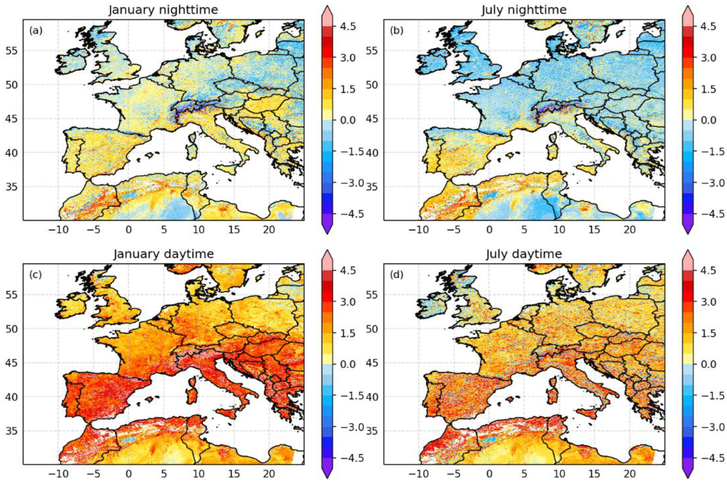
3.1. Monitoring 2018 Monthly Heat Extremes Using MSG LST

Spatial patterns of monthly anomaly values of MSG LST during 2018 over Europe are shown in Figure 3. High positive anomaly values are observed over Northern and Central Europe for all the months of 2018, except February and March which exhibited a spatial pattern of strong negative anomaly values over all of Europe (Turkey and part of the Balkans being exceptions); more specifically, the higher values over central and Northeastern Europe in March and Northern, Eastern Europe and alpine regions in February. Although with weaker values, negative anomaly values are also present in Eastern European countries during November and December. Conversely, it is interesting to see the slightly negative anomalies observed over the Iberian Peninsula from February to July. Indeed, Figure 3 clearly shows that while the Iberian Peninsula were characterized by a relatively cool spring, Northern and Central European countries were affected by above-normal LST values from the beginning of spring up to mid-autumn. On the other hand, strong positive anomalies are observed in January, April, August, and October over the entire European region.

The pattern of positive anomaly values is persistent throughout the year, with higher and more persistent anomalies over Northern and Central Europe. Figure 4 shows the number of months that recorded the highest monthly MSG LST anomaly value between January and December 2018, from 2004 to 2019. A large spatial pattern shows more than four months (out of 12) with MSG LST monthly anomaly values which were record-breaking for the considered period. This pattern is observed over Estonia, Latvia, Lithuania, Poland, Germany, Check Republic, Sweden, British Isles, France, Switzerland, Austria, Slovakia, and Hungary, with hotspots of 7 months over Latvia and Lithuania. A large but sparse spatial pattern with 5 and 6 anomalous LST months covers Poland, Germany, Switzerland, and the Check Republic.

Figure 5 shows the monthly Number of Hot Days (NHD) for each month in 2018, computed using MSG LST over Europe. More than seven hot days are recorded over northern countries in May, June, and July; from July to October over Central Europe; and over Southeastern Europe in April. A lower number of hot days (up to 5, depending on the pixel) were observed over Southern Europe, namely the Iberian Peninsula in January, February, September, October, and December 2018. Although several months do present intense values (Figure 3) in terms of temperature anomalies, hot extremes occurred within a relatively short period. However, a highlight should be added for the fact that the determined NHD does not oblige the consecutiveness of the hot days.

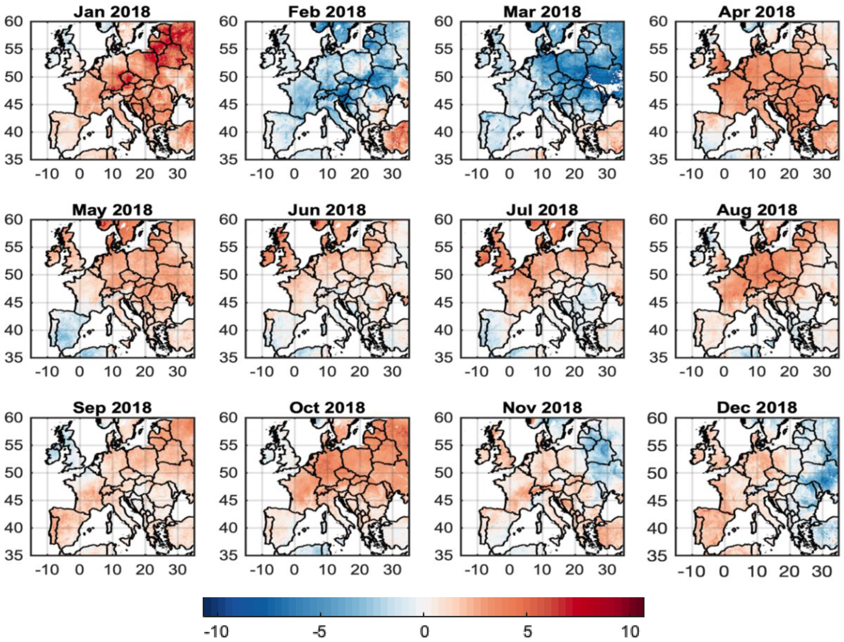
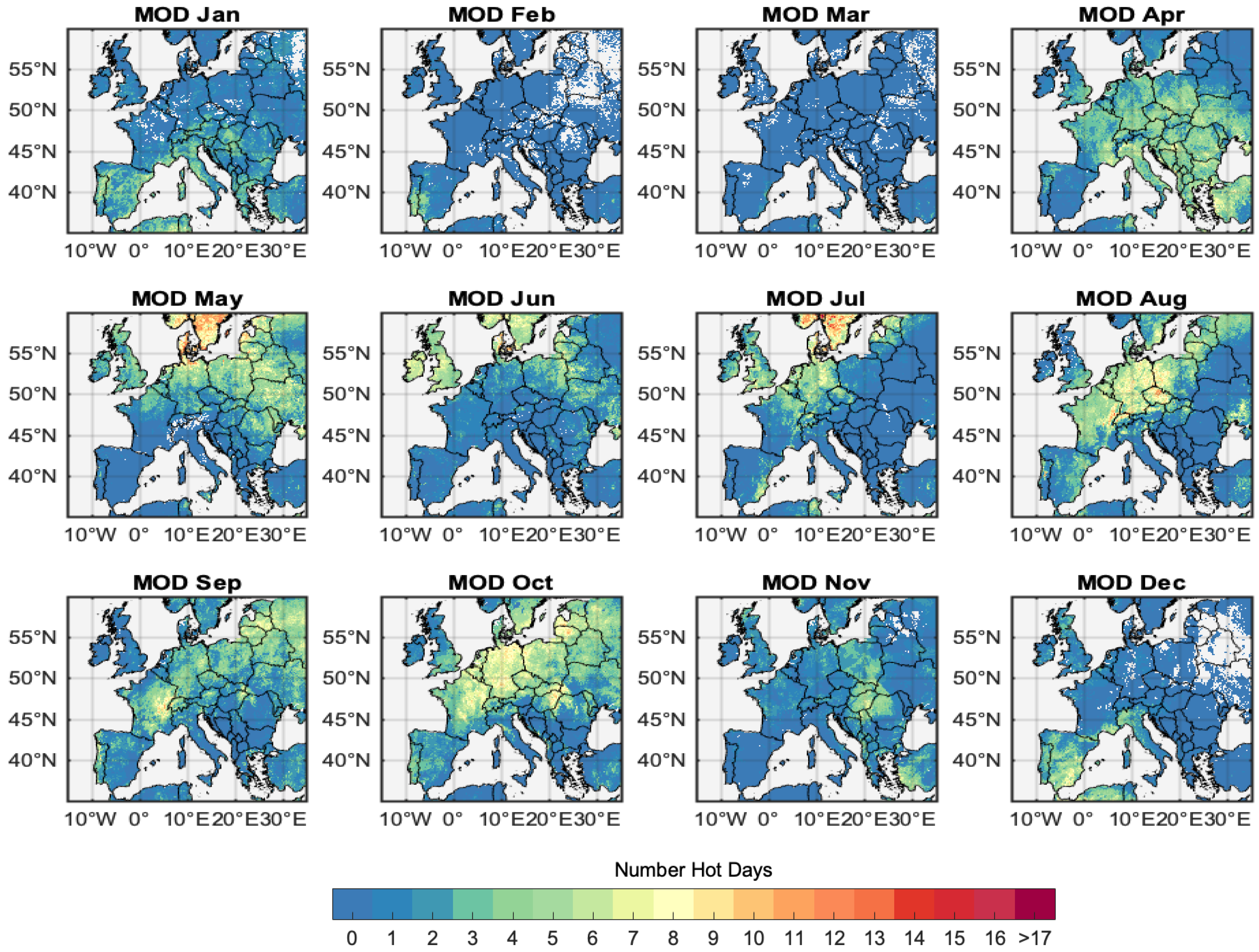
3.2. Monitoring 2018 Monthly Heat Extremes Using MODIS LST

A similar analysis is performed using MODIS LST. Figure 6 shows the monthly LST anomalies, using the full MYD11 data record, showing similar general patterns observed as when using LST from MSG. Strong positive LST anomalies over Central Europe, with notable exceptions for February and March; the same pattern of negative anomalies over Iberia before the summer months and the same pattern of West–East anomaly gradient in December. However, there are a few notable differences, namely: (1) there are more pixels with missing values for MODIS data since these are based on roughly two overpasses per day, while the higher sampling of MSG allows for better sampling in this case, increasing the probability of obtaining clear-sky observations over any given region (particularly relevant in areas with high cloud cover); (2) MSG LST also shows relatively higher anomalies in January over Central and Northeastern Europe. In February and March, some differences appear over regions with significant negative anomalies, which could indicate different treatment of snow or cloudy pixels over snow for each dataset. In July and August, the region of high LST anomalies seems more widespread over Central Europe for MSG LST when compared to the MODIS maps.

The number of months in 2018 with average MODIS LSTs corresponding to the highest anomaly across the whole data record is shown in Figure 7. Again, as with to Figure 4, record-breaking LST anomalies were reached in 4 months over large areas of Northern Europe, with some pixels over the Baltic countries and Poland showing record-breaking LSTs over five months. In the Mediterranean regions, the overall pattern is more scattered, showing regions where no record-breaking LSTs were measured and others where 2018 obtained the highest values in 2–3 months.

Finally, the NHD (i.e., number of days where LST exceeded the 90th percentile for that pixel) are shown in Figure 8. Similar to the results obtained with MSG, a few hot days (up to 5, depending on the pixel) were observed over Southern Europe in January and February, particularly over Iberia.

It should be noted that the number of missing values is again higher in the latter maps when compared to those in Figure 5, which can be explained by the fact that daily values from MSG are obtained from 15-min data, while MODIS (MYD11) usually relies on two measurements per day. Very high NHD (between 7 and 12) were observed in May and July over Northern Europe, whereas, over Central Europe, relatively high numbers were observed from April to October (although with some relief in June).

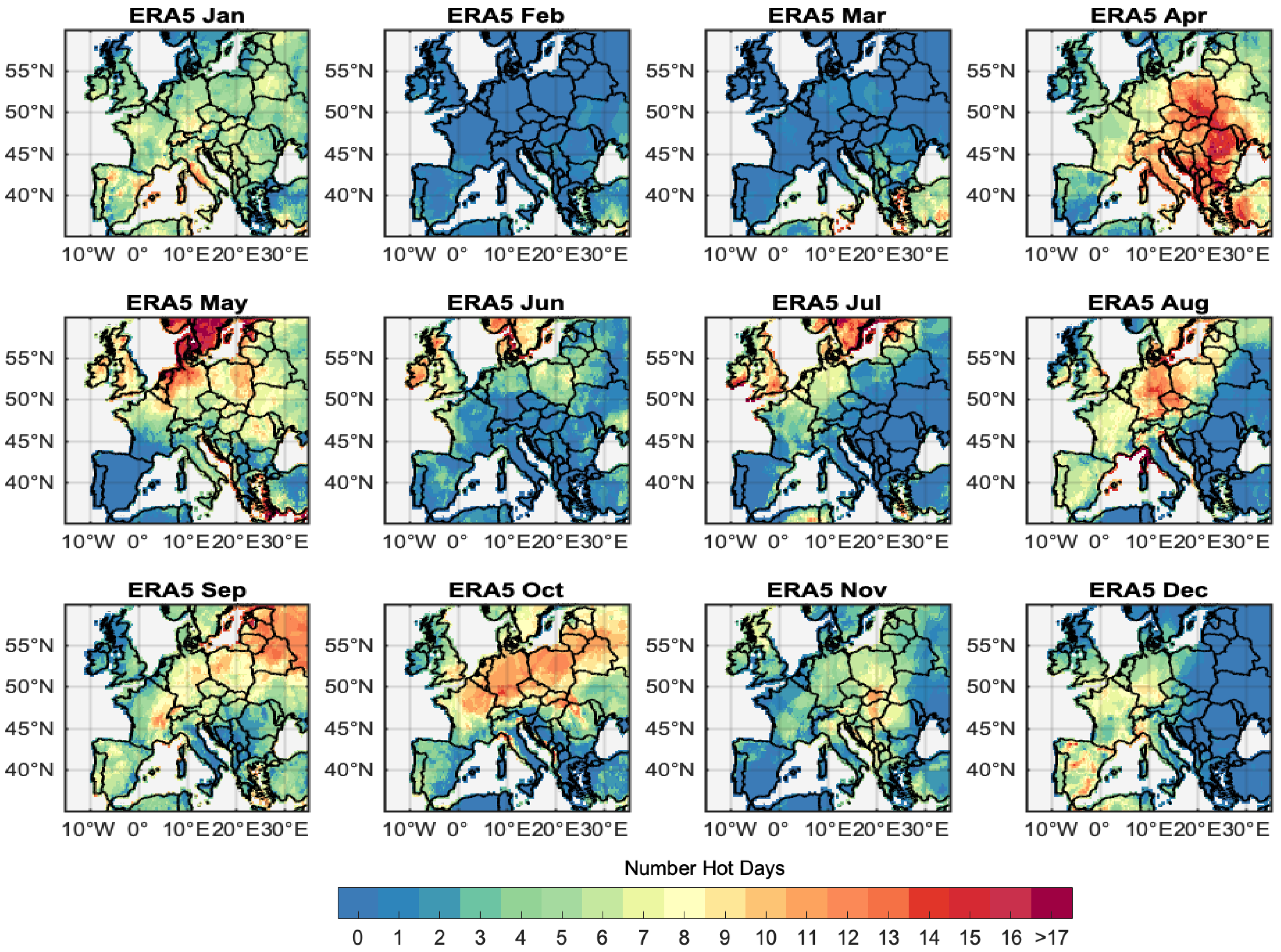
3.3. Monitoring 2018 Monthly Hot Extremes Using ERA5 T2m

The spatial patterns of monthly anomaly values of 2 m air temperature (T2m) from ERA5 during 2018, considering as reference period the one used for the MSG LST dataset (i.e., 2004–2019), are shown in Figure 9. For a better visual comparison with LST maps, the values over the ocean were masked. The spread pattern of negative anomaly values during February and March is evident, as well as the local minima in Eastern Northern Europe in November and December. On the other hand, spread patterns of high positive anomaly values are observed in January, April, and May, except over Iberia. Smaller but positive monthly anomaly values are observed from June to September. Results considering the 40-year period of T2m (1979–2019) exhibit very similar patterns (Figure S1), showing slightly higher positive anomaly values and lower negative anomaly values, in November and December, respectively.

The number of months in 2018 with monthly T2m corresponding to the highest anomaly in the common period is shown in Figure 10. Record-breaking T2m anomalies were reached in 3 months over wide Northern and Central Europe areas. In the Mediterranean regions, the overall pattern is more scattered with regions where no record-breaking LSTs were measured to areas where it occurred 1–2 months (Figure S2). The spatial pattern obtained when considering the full (40-year) reanalysis period is very similar, despite showing, as expected, relatively smaller areas with three months of record-breaking temperature anomalies. Southern Europe presents a large pattern of almost no record-breaking monthly temperature anomalies.

Finally, the NHDs obtained using T2m are shown in Figure 11. Large patterns of more than eight hot days per month were observed over Northern and Central Europe from April to October. April shows the most widespread maxima strongly affecting the Southeastern European countries. The lowest number of hot days (up to 6) were observed over Southern Europe, namely the Iberian Peninsula, in January, August, September, and December 2018.

Finally, the NHD obtained using T2m are shown in Figure 11. Large patterns of more than eight hot days per month were observed over Northern and Central Europe from April to October. April shows the most widespread maxima strongly affecting the Southeastern European countries. The lowest number of hot days (up to 6) were observed over Southern Europe, namely the Iberian Peninsula, in January, August, September, and December 2018. When the 40-year period was analyzed (Figure S3), similar patterns were observed, with large areas with more than nine hot days per month in central and northern European countries in April, August, and September, and up to 6 days in southern countries, namely in October and winter months.

4. Discussion

Climate monitoring applications rely mainly on in situ observations and reanalysis [27,28,29], due to the availability of long temporal coverage. However, time-series obtained from high-quality satellite imagery are reaching temporal spans compatible with climate studies. Nevertheless, the accuracy and precision of remote sensing products and the data records’ high decadal stability are crucial factors to account for if we aim to use such datasets to monitor climate extremes, such as heat/cold waves, and droughts, among others.

The consistency between the MSG LST and MODIS LST datasets was assessed for the LST reprocessing period (2014–2015) by comparing the two datasets over a spatial domain including Europe and North Africa regions (15°W–25°E, 20°N–60°N) for January and July (day and night times). In general, MSG LST is warmer than MODIS LST. MSG LST values in Northern Europe are mostly colder in the nighttime, particularly in July. In contrast, MSG LST in Mediterranean regions is generally warmer even in the nighttime (exception for desert regions), with differences exceeding 3 K over some areas in daytime. The differences could be related to several factors, namely differences in the prescribed surface emissivity [30]. On the other hand, viewing geometry from MODIS changes in each overpass, while SEVIRI is mainly in the same position all the time, meaning that it views the same scene with mostly the same viewing angle from the south and therefore favoring the measurement of LST over sun-illuminated surfaces. There are many reasons why infrared-based LST estimates may differ: uncertainties in the retrievals tend to increase with viewing angle, on one hand, while the surface emissivity and the actual temperature of the surface change with viewing and illumination geometry; on the other hand, the use of different surface emissivities may introduce systematic errors (e.g., [18]). In this case, the differences in the seasonal representation of surface emissivity in MODIS and MSG products may explain the higher bias in January compared with July. The more recently released MYD21 product comprises LST and emissivity derived from MODIS onboard Aqua retrieved using the Temperature Emissivity Separation (TES) algorithm [31]. Preliminary results have shown that MYD21 LST estimates tend to be closer to those estimated by the LSA-SAF from MSG. However, the purpose of this work is to demonstrate the use of satellite-based LST products to identify and monitor the signature of heatwaves at regional-to-continental scales: both MYD11 and MYD21 could be used for that purpose. However, the use of product anomalies or other statistics defined by each product distribution allows the use of both climate monitoring and the assessment of extreme warm events, as considered here.

CDRs are produced and maintained to provide a long and homogeneous time-series of relevant climate monitoring variables. Conventional in situ data, gridded datasets, and reanalysis are still of utmost usefulness for climate studies. Their intrinsic characteristics, however, limit them. For instance, well-maintained in situ weather stations have provided the longest reliable time-series datasets. Their spatial coverage and representativity are always limited, especially for highly varying parameters such as surface temperature or precipitation. There are also much more of these stations within the most developed countries than in less developed countries [32]. Gridded datasets have been developed to overcome the spatial coverage limitation of individual stations [33]. However, interpolation of near-surface meteorological fields is always tricky, as their spatial variability is modulated not only by each synoptic situation but also by environmental factors such as land cover, orography, and distance to water bodies or urban areas, among others. Several such datasets have been discussed in the literature and used for climate studies (e.g., the ECAD-EOBS dataset, [32]). These datasets may be multi-variable, which is helpful for process studies. Reanalysis datasets overcome most of the limitations in these simpler gridded datasets, not only through the assimilation of all sorts of measurements (e.g., collected by conventional in situ stations, satellites, airplanes, ships, GNSS) while minimizing their relative differences, but also because they make use of a physically constrained model which allows filling in those grid boxes/timeslots where fewer observations were available.

Although acknowledging the relevance of reanalysis in providing a consistent dataset of atmospheric and surface variables, through the assimilation of observations from numerous sources, there is a growing interest in the development of high-quality observational datasets [34] that are independent and free of the necessary assumptions made in models. This is particularly the case for land surface variables, including temperature, moisture, or surface fluxes, as these are strongly influenced by the representation of surface characteristics in model land schemes (e.g., [35]).

This kind of issue puts the satellite CDRs into a privileged position, as they can provide comprehensive spatial coverage while minimizing the dependence on model parameters (and thus decreasing uncertainty due to model deficiencies). However, given the opacity of clouds to infrared radiation, infrared remote sensors can only measure surface parameters over clear-sky conditions, i.e., all satellite LST products considered here are available under clear sky conditions only. Compared to other datasets, this is a major caveat since it reduces spatial coverage and increases the uncertainty due to the misclassification of cloudy pixels. It introduces the so-called clear-sky bias [36], which is related to the fact that surface temperatures below clouds are generally very different from surrounding pixels that are under clear skies (e.g., [37]). The bias values are about 2–8 K in the mid-latitudes in the daytime (due to increased solar radiation over a clear sky) and −2 K in the nighttime due to the greenhouse effect below clouds leading to less radiative cooling of the surface. This effect needs to be accounted for when using MSG LSTs for climate monitoring. However, it expected a very low, even negligible, impact of the clear-sky bias on heat extremes assessment, as over Europe a heatwave is usually associated with high values of solar radiation and therefore very low cloud cover. Therefore, what is shown in Figure 3, Figure 4, Figure 5, Figure 6, Figure 7, Figure 8, Figure 9, Figure 10 and Figure 11 is that, apart from some small differences, the general patterns are very similar. The same analysis was also applied to other important heat extremes over Europe, namely 2006, 2015 and 2017 years, with very good results. However, we have chosen the 2018 heat extremes to be analyzed here, because of the exceptionally wide area and total duration of the positive temperature anomalies observed that year: a large spatial pattern of pixels was affected by extreme surface temperature values for more than 5 months.

Several datasets retrieved from reanalysis, models, and satellite information have been used to evaluate the role of temperature, precipitation, evapotranspiration, soil moisture, and radiation on vegetation productivity and crop yields [1,2,3,4,11,12,13,14]. LST is a radiative skin temperature of the land surface and is sensitive to surface soil water content due to its influence on the surface heating process [38]. On the other hand, several authors have shown the role played by soil moisture in the partition of energy into sensible and latent heat fluxes and consequently in its control of evapotranspiration [39,40,41]. Moreover, this effect depends on vegetation cover [41], and given its role in the surface energy balance, it has been shown that infrared LST daily amplitude is very closely linked to the surface energy partition and evaporative regimes [34]. Due to their different physical nature, LST and T2m are significantly different in terms of the response to atmospheric conditions and the diurnal cycle. However, a good agreement is found in some circumstances when the spatial and temporal variability is similar, and the significant patterns of T2m and LST are consistent at large spatial scales [42]. The agreement between LST and T2m is better during the night due to the negligible effect of shortwave radiation on the thermal infrared signal. In contrast, the complex energy balance at the surface increases the difference between T2m and LST during the day as LST responds almost instantaneously to the excess net radiation, while the air above it has a slower response, mainly through the sensible heat flux and from the absorption of longwave radiation, both coming from the surface.

Several authors have studied the extreme conditions in 2018 in Europe. Proxy-based seasonal paleoclimate reconstructions allow identifying only nine extreme summer conditions comparable with 2018: one in 2003, three in the 12th century, and five in the 16th century [3]. The exceptionality of the 2018 year was assessed here using monthly anomalies and the number of heat days (NHD) using LST from satellite (MSG and MODIS) and 2m temperature from ERA5 (T2m). Spatial patterns of positive monthly anomalies, record-breaking anomalies, and NHD obtained using LST Data Records from MSG LST are in good agreement with the ones obtained with MODIS LST and T2m ERA5 datasets. In general, the monthly anomalies obtained with MSG LST are higher than those obtained using MODIS LST and T2m, namely the number of record-breaking observed anomalous values. The main differences may be related to the use of 15-min MSG LST data to obtain monthly LST values compared to the daily observation of MODIS LST (obtained close to 13:30 UTC) and the spatial resolution of the T2m reanalysis dataset (0.25 degrees). The presence of clouds may also have a higher impact on MODIS LST estimation of monthly LST compared with MSG LST due to the large differences in the temporal sampling and, therefore, in the number of potentially clear-sky observations.

Results using MSG LST also pointed out the exceptional temperatures observed over Scandinavia, Central Europe during most of the year (except February and March), over the British Isles from April to August and over the Iberian Peninsula from August to December, as also demonstrated by [2]. However, slightly negative anomalies were found over the Iberian Peninsula from February to July. The area affected by more than four months showing record-breaking LST values in the 2004–2019 period is very large, emphasizing how extreme, widespread, and temporally persistent the observed temperatures were, which is in accordance with previous studies that highlight the exceptional character of the 2018 summer that surpassed the 2003 and 2010 heatwave events [2,3,4]. Central and Eastern Europe were struck by a major heatwave in spring and summer and concurrent extreme dry and brightening conditions, whereas, in Southern Europe, some precipitation occurred [11]. The authors in [4] distinguish the 2018 summer heatwave from the 2010 and 2003 events and related the difference with the legacy effect of the extreme warming and brightening, although only moderately dry spring and with the quick transition between a wet winter to an extremely dry summer. In contrast, Southern Europe experienced one of the wettest summers and one of the two wettest springs since 1950 [11], particularly the anomalous wet conditions in March associated with a persistent negative North Atlantic Oscillation pattern [43]. Regional asymmetries in summer ecosystem carbon fluxes were also found mainly associated with the legacy impact of spring growth and water use efficiency linked with vegetation types. However, a clear positive impact on vegetation productivity was found in Southern Europe, where summer was wetter than usual [4].

The exceptional and prolonged heat extremes were associated with crop losses of up to 50% in Switzerland, the British Isles, Russia, and Germany; with the unusual cases of rails buckling and roads melting in British Isles and the Netherlands [1,3]. In 2018, Northern and Eastern Europe experienced significant crop failures associated with extremely dry conditions combined with high temperatures between March and August [11]. The adverse impact of hot and dry summers on vegetation may be impaired by a soil moisture deficit in previous months and the early onset of the growing season in spring. Low precipitation and/or high temperature and shortwave radiation in spring increase evaporation rate leading to soil moisture deficit. Hot and dry springs can increase the sensitivity of vegetation to heat and dry extremes [12]. Bad seasons for wheat yield in France and Germany are linked with low precipitation, high maximum temperature, and high vapor pressure deficit in the growing season (May–July). It should be noted that in the growing season, crop development is constrained by the compound warm and dry conditions that lead to yield and quality losses. Therefore, the compounding effect of meteorological conditions during the growing season is an essential driver for European wheat losses and may severely influence food security [12]. In contrast, higher than usual crop yields were recorded in Southern Europe, mainly associated with favorable spring wet conditions [11]. However, the positive anomaly values and NHD observed in Southern European countries, namely in summer and fall, were associated with the exceptional 2018 fire season that struck Portugal, Spain, and Greece. However, the intensity and relevance of the observed early August Iberian heatwave were masked by relatively wet and cool conditions in June–July 2018 that resulted in near-average seasonal mean temperature anomalies over the region [44]. However, exceptional absolute temperatures were recorded, mainly over Portugal, where all-time records were broken in many places, including most of those standing since the 2003 mega heatwave [44,45]. Consequently, large areas of intact forests were destroyed by devastating fires [2]. Exceptional fire activity was observed in countries with no history of large fires, such as Sweden, Norway, Finland, and Latvia [46].

The assessment of extreme heat events, based on NHD and consequently relying on maximum air temperature and LST, presents different features compared with the monthly median anomalies and when considering other datasets. In fact, the high number of monthly NHD values is evident mainly from May to August in Northern European countries. The NHD is also high in April, September, and October, respectively, over Southeastern, France, and Central Europe. The spatial patterns of exceptional heat events using monthly anomalies and maximum (used to estimate the NHD) temperatures are not exactly equal, as expected due to the different mean and maximum temperature behavior. On the other hand, the monthly NHD seems higher for the reanalysis dataset. This difference may be related to the different daily moments when the temperature peak is obtained in the case of radiometric temperatures (LST) and air temperature [47].

The complex relationship between air temperature, soil moisture, evapotranspiration, radiation, and vegetation productivity that makes the extreme 2018 year so exceptional seems to be better captured when using LST monthly anomalies derived from a geostationary satellite that allows characterizing the diurnal cycle than to use MODIS LST or T2m. The number of monthly record anomalies obtained using MSG LST in 2018 (with respect to the 2004–2019 period) is higher than for MODIS LST or for ERA5 T2m, and the spatial pattern allows identifying the more severely affected regions in Northern and Central Europe mentioned in the above works, therefore highlighting the combined effect of drought and heat extremes. The encouraging results on monitoring heat extremes during 2018 highlight the ability and usefulness of MSG LST for this purpose. The added value of using these satellite datasets has assumed a higher role in the last decade, due to the increase in the frequency and intensity of heat extremes over the past few decades in Europe [29,48,49,50,51] and the need to follow the evolution of such events in near-real time. Moreover, due to the projected increase of these extreme events [29,50,51], combined with larger exposure, an exceptional risk increase to humans and ecosystems is expected [52].

Finally, we would like to highlight the importance of considering the interplay between different climate extremes when analyzing the impacts on other sectors, such as crop losses and wildfires in Europe. The availability of other CDRs, such as vegetation parameters (e.g., Leaf Area Index, LAI), evapotranspiration, radiation, and heat fluxes from MSG with Near-Real Time updating opens a large opportunity to develop tools to monitor the evolution of extreme heat events alone or compounding with other extreme events and allow decision-makers to anticipate and adopt strategies to prevent future losses.

5. Conclusions

Over the European domain, MSG LST generally yields higher temperatures than the MODIS LST product considered in this study, the MYD11 (collection 6). Some exceptions were also found. Northern Europe is dominated by negative values of the difference between the two LST products in the nighttime, particularly in July. On the other hand, Mediterranean regions are generally warmer as measured by MSG LST even in the nighttime, while desert regions are colder. MSG LST surpasses MODIS LST in the daytime, with differences over 4 K in some Mediterranean areas. In the daytime, median differences decrease in July for all land covers except for grasslands and, to a lesser extent, closed shrublands and barren, whereas, in the nighttime, median differences are much smaller and less scattered. However, such systematic discrepancies will not have a significant impact on the use of LST anomalies, of any of those products, to assess the extent of record hot events.

Spatial patterns of positive monthly anomalies, record-breaking anomalies, and the NHD obtained using MSG LST agree with the ones obtained with MODIS LST and T2m ERA5 datasets and with previous studies. In general, the monthly anomalies obtained with MSG LST are higher than those obtained using MODIS LST and T2m, namely the number of anomalous values observed. On the other hand, the monthly NHD seems higher for the reanalysis dataset.

The spatial pattern of the number of monthly record anomalies (considering the 2004–2019 reference period) obtained using MSG LST permits identifying the regions in Northern and Central Europe affected by the complex phenomena that occurred in 2018, which resulted from the combined effect of an extreme heatwave in spring and summer with extensive dry conditions. This result reinforces the idea that climate data records of vegetation parameters, radiation, and heat fluxes obtained from geostationary satellites, and now available for almost 20 years, seem to be suitable data sources for evaluating single, combined, or cascading climate extremes.

The near-real-time availability of satellite data to monitor and evaluate heat extremes and the potential impacts on agricultural, human health, and other social sectors enables a faster application of measures to mitigate those impacts. Therefore, the encouraging results on monitoring heat extremes during 2018 highlight the ability and usefulness of MSG LST for heat extremes analysis.

References

1. Vogel, M.M.; Zscheischler, J.; Wartenburger, R.; Dee, D.; Seneviratne, S.I. Concurrent 2018 hot extremes across Northern Hemisphere due to human-induced climate change. Earth’s Future 2019, 7, 692–703. [Google Scholar] [CrossRef]
2. Barriopedro, D.; Sousa, P.M.; Trigo, R.M.; García-Herrera, R.; Ramos, A.M. The exceptional Iberian heatwave of summer 2018. Bull. Am. Meteorol. Soc. 2020, 101, S29–S34. [Google Scholar] [CrossRef] [Green Version]
3. Toreti, A.; Belward, A.; Perez-Dominguez, I.; Naumann, G.; Manfron, G.; Jürg, L.; Cronie, O.; Seguini, L.; Manfron, F.; Lopez-Lozano, R.; et al. The exceptional 2018 European water seesaw calls for action on adaptation. Earth’s Future 2019, 7, 652–663. [Google Scholar] [CrossRef]
4. Bastos, A.; Ciais, P.; Friedlingstein, P.; Sitch, S.; Pongratz, J.; Fan, L.; Wigneron, J.P.; Weber, U.; Reichstein, M.; Fu, Z.; et al. Direct and seasonal legacy effects of the 2018 heat wave and drought on European ecosystem productivity. Sci. Adv. 2020, 6, eaba2724. [Google Scholar] [CrossRef]
5. Russo, A.; Gouveia, C.M.; Dutra, E.; Soares, P.M.M.; Trigo, R.M. The synergy between drought and extremely hot summers in the Mediterranean. Environ. Res. Lett. 2019, 14, 014011. [Google Scholar] [CrossRef]
6. Ribeiro, A.F.S.; Russo, A.; Gouveia, C.M.; Pires, C.A.L. Drought-related hot summer: A joint probability analysis in the Iberian Peninsula. Weather Clim. Extrem. 2020, 30, 100279. [Google Scholar] [CrossRef]
7. Robine, J.M.; Cheung, S.L.; Le Roy, S.; Van Oyen, H.; Griffiths, C.; Michel, J.P.; Herrmann, F.R. Death toll exceeded 70,000 in Europe during the summer of 2003. C. R. Biol. 2008, 331, 171–178. [Google Scholar] [CrossRef]
8. Barripedro, D.; Fisher, E.M.; Lutherbacher, J.; Trigo, R.M.; Garcia-Herrera, R. The hot summer of 2010: Redrawing the temperature record map of Europe. Science 2011, 332, 220–224. [Google Scholar] [CrossRef] [Green Version]
9. Seneviratne, S.; Donat, M.G.; Mueller, B.; Alexander, L.V. No pause in the increase of hot temperature extremes. Nat. Clim. Change 2014, 4, 161–163. [Google Scholar] [CrossRef]
10. Christidis, N.; Ciavarella, A.; Stott, P.A. Different ways of framing event attribution questions: The example of warm and wet winters in the United Kingdom similar to 2015/16. J. Clim. 2018, 31, 4827–4845. [Google Scholar] [CrossRef]
11. Beillouin, D.; Schauberger, B.; Bastos, A.; Ciais, P.; Makowski, D. Impact of extreme weather conditions on European crop production in 2018. Philos. Trans. R. Soc. B 2020, 375, 20190510. [Google Scholar] [CrossRef] [PubMed]
12. Bevacqua, E.; De Michele, C.; Manning, C.; Couasnon, A.; Ribeiro, A.F.; Ramos, A.M.; Vignotto, E.; Bastos, A.; Blesić, S.; Durante, F.; et al. Guidelines for studying diverse types of compound weather and climate events. Earth’s Future 2021, 9, e2021EF002340. [Google Scholar] [CrossRef]
13. Drouard, M.; Kornhuber, K.; Woollings, T. Disentangling dynamic contributions to summer 2018 anomalous weather over Europe. Geophys. Res. Lett. 2019, 46, 12537–12546. [Google Scholar] [CrossRef] [Green Version]
14. Liu, X.; He, B.; Guo, L.; Huang, L.; Chen, D. Similarities and differences in the mechanisms causing the European summer heatwaves in 2003 2010, and 2018. Earth’s Future 2020, 8, e2019EF001386. [Google Scholar] [CrossRef] [Green Version]
15. Christidis, N.; Jones, G.S.; Stott, P.A. Dramatically increasing chance of extremely hot summers since the 2003 European heatwave. Nat. Clim. Change 2015, 5, 46–50. [Google Scholar] [CrossRef]
16. Norman, J.M.; Becker, F. Terminology in thermal infrared remote sensing of natural surfaces. Agric. For. Meteorol. 1995, 77, 153–166. [Google Scholar] [CrossRef]
17. Guillevic, P.; Göttsche, F.; Nickeson, J.; Hulley, G.; Ghent, D.; Yu, Y.; Trigo, I.; Hook, S.; Sobrino, J.A.; Remedios, J.; et al. Land Surface Temperature Product Validation Best Practice Protocol: Version 1.0. In Best Practice for Satellite-Derived Land Product Validation; Guillevic, P., Göttsche, F., Nickeson, J., Román, M., Eds.; Land Product Validation Subgroup (WGCV/CEOS): Washington, DC, USA, 2017; p. 60. [Google Scholar] [CrossRef]
18. Trigo, I.F.; Ermida, S.E.; Martins, J.P.M.; Gouveia, C.M.; Göttsche, F.-M.; Freitas, S.C. Validation and consistency assessment of land surface temperature from geostationary and polar orbit platforms: SEVIRI/MSG and AVHRR/Metop. ISPRS J. Photogramm. Remote Sens. 2021, 175, 282–297. [Google Scholar] [CrossRef]
19. Gouveia, C.; Martins, J.P.A.; Trigo, I.F.; Coelho, S.; Göttsche, F.; Olesen, F. Validation Report Land Surface Temperature (LSA-050); Satellite Application Facility on Land Surface Analysis (LSA SAF), EUMETSAT: Darmstadt, Germany, 2018; (SAF/LAND/IM/VR_MLST-R/1.0). [Google Scholar]
20. Freitas, S.C.; Trigo, I.F.; Bioucas-Dias, J.M.; Goettsche, F.-M. Quantifying the Uncertainty of Land Surface Temperature Retrievals from SEVIRI/Meteosat. IEEE Trans. Geosci. Remote Sens. 2010, 48, 523–534. [Google Scholar] [CrossRef] [Green Version]
21. Goettsche, F.-M.; Olesen, F.-S.; Trigo, I.F.; Bork-Unkelbach, A.; Martin, M.A. Long term validation of land surface temperature retrieved from MSG/SEVIRI with continuous in-situ measurements in Africa. Remote Sens. 2016, 8, 410. [Google Scholar] [CrossRef] [Green Version]
22. Trigo, I.F.; Peres, L.F.; DaCamara, C.C.; Freitas, S.C. Thermal land surface emissivity retrieved from SEVIRI/Meteosat. IEEE Trans. Geosci. Remote Sens. 2008, 46, 307–315. [Google Scholar] [CrossRef]
23. Madhavan, S.; Brinkmann, J.; Wenny, B.N.; Wu, A.; Xiong, X. Evaluation of VIIRS and MODIS Thermal Emissive Band Calibration Stability Using Ground Target. Remote Sens. 2016, 8, 158. [Google Scholar] [CrossRef] [Green Version]
24. Wan, Z.; Zhang, Y.; Zhang, Y.Q.; Li, Z.-L. Validation of the land-surface temperature products retrieved from Moderate Resolution Imaging Spectroradiometer data. Remote Sens. Environ. 2002, 83, 163–180. [Google Scholar] [CrossRef]
25. Wan, Z. New refinements and validation of the collection-6 MODIS land-surface temperature/emissivity product. Remote Sens. Environ. 2014, 140, 36–45. [Google Scholar] [CrossRef]
26. Hersbach, H.; Bell, B.; Berrisford, P.; Hirahara, S.; Horányi, A.; Muñoz-Sabater, J.; Nicolas, J.; Peubey, C.; Radu, R.; Schepers, D.; et al. The ERA5 global reanalysis. Q. J. R. Meteorol. Soc. 2020, 146, 1999–2049. [Google Scholar] [CrossRef]
27. Baldi, M.; Dalu, G.; Maracchi, G.; Pasqui, M.; Cesarone, F. Heat waves in the Mediterranean: A local feature or a larger-scale effect? Int. J. Climatol. 2006, 26, 1477–1487. [Google Scholar] [CrossRef] [Green Version]
28. Perkins-Kirkpatrick, S.E.; Lewis, S.C. Increasing trends in regional heatwaves. Nat. Commun. 2020, 11, 3357. [Google Scholar] [CrossRef]
29. Russo, S.; Sillmann, J.; Fischer, E. Top ten European heatwaves since 1950 and their occurrence in the coming decades. Environ. Res. Lett. 2015, 10, 124003. [Google Scholar] [CrossRef]
30. Qian, Y.G.; Li, Z.L.; Nerry, F. Evaluation of land surface temperature and emissivities retrieved from MSG/SEVIRI data with MODIS land surface temperature and emissivity products. Int. J. Remote Sens. 2013, 34, 3140–3152. [Google Scholar] [CrossRef]
31. Hulley, G.; Veraverbeke, S.; Hook, S. Thermal-based techniques for land cover change detection using a new dynamic MODIS multispectral emissivity product (MOD21). Remote Sens. Environ. 2014, 140, 755–765. [Google Scholar] [CrossRef]
32. Cornes, R.; van der Schrier, G.; van den Besselaar, E.J.M.; Jones, P.D. An Ensemble Version of the E-OBS Temperature and Precipitation Datasets. J. Geophys. Res. Atmos. 2018, 123, 9391–9409. [Google Scholar] [CrossRef] [Green Version]
33. Herrera, S.; Cardoso, R.M.; Soares, P.M.; Espírito-Santo, F.; Viterbo, P.; Gutiérrez, J.M. Iberia01: A new gridded dataset of daily precipitation and temperatures over Iberia. Earth Syst. Sci. Data 2019, 11, 1947–1956. [Google Scholar] [CrossRef] [Green Version]
34. Feldman, A.F.; Gianotti, D.J.S.; Trigo, I.F.; Salvucci, G.D.; Entekhabi, D. Land-atmosphere drivers of landscape-scale plant water content loss. Geophys. Res. Lett. 2020, 47, e2020GL090331. [Google Scholar] [CrossRef]
35. Nogueira, M.; Boussetta, S.; Balsamo, G.; Albergel, C.; Trigo, I.F.; Johannsen, F.; Miralles, D.G.; Dutra, E. Upgrading land-cover and vegetation seasonality in the ECMWF coupled system: Verification with FLUXNET sites, METEOSAT satellite land surface temperatures, and ERA5 atmospheric reanalysis. J. Geophys. Res. Atmos. 2021, 126, e2020JD034163. [Google Scholar] [CrossRef]
36. Ermida, S.L.; Trigo, I.F.; DaCamara, C.C.; Jiménez, C.; Prigent, C. Quantifying the Clear-Sky Bias of Satellite Land Surface Temperature Using Microwave-Based Estimates. J. Geophys. Res. Atmos. 2019, 124, 844–857. [Google Scholar] [CrossRef]
37. Martins, J.P.A.; Trigo, I.F.; Ghilain, N.; Jimenez, C.; Göttsche, F.-M.; Ermida, S.L.; Olesen, F.-S.; Gellens-Meulenberghs, F.; Arboleda, A. An All-Weather Land Surface Temperature Product Based on MSG/SEVIRI Observations. Remote Sens. 2019, 11, 3044. [Google Scholar] [CrossRef] [Green Version]
38. Zhao, W.; Li, Z.L. Sensitivity Study of Soil Moisture on the Temporal Evolution of Surface Temperature over Bare Surfaces. Int. J. Remote Sens. 2013, 34, 3314–3331. [Google Scholar] [CrossRef]
39. Boulet, G.; Mougenot, B.; Lhomme, J.P.; Fanise, P.; Lili-Chabaane, Z.; Olioso, A.; Bahir, M.; Rivalland, V.; Jarlan, L.; Merlin, O.; et al. The SPARSE model for the prediction of water stress and evapotranspiration components from thermal infra-red data and its evaluation over irrigated and rainfed wheat. Hydrol. Earth Syst. Sci. 2015, 19, 4653–4672. [Google Scholar] [CrossRef] [Green Version]
40. Gokmen, M.; Vekerdy, Z.; Verhoef, A.; Verhoef, W.; Batelaan, O.; Tol, C.V.D. Remote Sensing of Environment Integration of soil moisture in SEBS for improving evapotranspiration estimation under water stress conditions. Remote Sens. Environ. 2012, 121, 261–274. [Google Scholar] [CrossRef]
41. Ait Hssaine, B.; Merlin, O.; Ezzahar, J.; Ojha, N.; Er-Raki, S.; Khabba, S. An evapotranspiration model self-calibrated from remotely sensed surface soil moisture, land surface temperature and vegetation cover fraction: Application to disaggregated SMOS and MODIS data. Hydrol. Earth Syst. Sci. 2020, 24, 1781–1803. [Google Scholar] [CrossRef] [Green Version]
42. Jin, M.; Dickinson, R.E. Land surface skin temperature climatology: Benefitting from the strengths of satellite observations. Environ. Res. Lett. 2010, 5, 044004. [Google Scholar] [CrossRef] [Green Version]
43. Ayarzagüena, B.; Barriopedro, D.; Garrido-Perez, J.M.; Abalos, M.; Cámara, A.; García-Herrera, R.; Calvo, N.; Ordóñez, C. Stratospheric connection to the abrupt end of the 2016/2017 Iberian drought. Geophys. Res. Lett. 2018, 45, 12639–12646. [Google Scholar] [CrossRef] [Green Version]
44. Sousa, P.M.; Barriopedro, D.; Ramos, A.M.; García-Herrera, R.; Espírito-Santo, F.; Trigo, R.M. Saharan air intrusions as a relevant mechanism for Iberian heatwaves: The record breaking events of August 2018 and June 2019. Weather Clim. Extrem. 2019, 26, 100224. [Google Scholar] [CrossRef]
45. IPMA—Instituto Português do Mar e da Atmosfera, I.P. Resumo Climatológico—Agosto de 2018; IPMA: Lisbon, Portugal, 2018. [Google Scholar]
46. Yiou, P.; Cattiaux, J.; Faranda, D.; Kadygrov, N.; Jézéquel, A.; Naveau, P.; Ribes, A.; Robin, Y.; Thao, S.; van Oldenborgh, G.J.; et al. Analyses of the Northern European summer heatwave of 2018. Bull. Am. Meteorol. Soc. 2020, 101, S35–S40. [Google Scholar] [CrossRef] [Green Version]
47. Good, E.J. An in situ-based analysis of the relationship between land surface “skin” and screen-level air temperatures. J. Geophys. Res. Atmos. 2016, 121, 8801–8819. [Google Scholar] [CrossRef]
48. Spinoni, J.; Naumann, G.; Vogt, J.; Barbosa, P. Meteorological Droughts in Europe: Events and Impacts—Past Trends and Future Projections; EUR 27748 EN; Publications Office of the European Union: Luxembourg, 2016; Available online: https://op.europa.eu/en/publication-detail/-/publication/a99deb15-d92e-11e5-8fea-01aa75ed71a1/language-en (accessed on 14 July 2022).
49. Sánchez-Benítez, A.; García-Herrera, R.; Barriopedro, D.; Sousa, P.M.; Trigo, R.M. June 2017: The earliest European summer mega-heatwave of reanalysis period. Geophys. Res. Lett. 2018, 45, 1955–1962. [Google Scholar] [CrossRef]
50. Turco, M.; Jerez, S.; Augusto, S.; Tarín-Carrasco, P.; Ratola, N.; Jiménez-Guerrero, P.; Trigo, R.M. Climate drivers of the 2017 devastating fires in Portugal. Sci Rep. 2019, 9, 13886. [Google Scholar] [CrossRef]
51. Lionello, P.; Scarascia, L. The relation of climate extremes with global warming in the Mediterranean region and its north versus south contrast. Reg. Environ. Chang. 2020, 20, 31. [Google Scholar] [CrossRef]
52. Seneviratne, S.I.; Nicholls, N.; Easterling, D.; Goodess, C.M.; Kana, S.; Kossin, J.; Luo, Y.; Marengo, J.; McInnes, K.; Rahimi, M.; et al. Changes in climate extremes and their impacts on the natural physical environment. In Managing the Risks of Extreme Events and Disasters to Advance Climate Change Adaptation: A Special Report of Working Groups I and II of the Intergovernmental Panel on Climate Change (IPCC); Chapter 3; Field, C.B., Barros, V., Stocker, T.F., Qin, D., Dokken, D.J., Ebi, K.L., Mastrandrea, M.D., Mach, K.J., Plattner, G.K., Allen, S.K., et al., Eds.; Cambridge University Press: Cambridge, UK, 2012; pp. 109–230. [Google Scholar]
Figure 1. The median difference between MSG LST and MODIS LST (in K) for (a) January—nighttime; (b) July—nighttime; (c) January—daytime, and (d) July—daytime for the period between 2004 and 2015.
Remotesensing 14 03470 g001
Figure 2. Statistics of the MSG LST-MODIS LST differences by land-cover type for January and July. Accuracy μ is represented with dots, and precision σ is represented as whiskers. Data for January is represented in purple, and for July in green. Separate statistics were computed for daytime (a) and nighttime (b). The numbers above the x-axis represent the number of matchups (i.e., MSG LST-MODIS LST valid pairs) used in January and June over each land-cover, respectively.
Remotesensing 14 03470 g002
Figure 3. Monthly anomaly values of MSG LST during 2018 over Europe, with respect to 2004–2019.
Remotesensing 14 03470 g003
Figure 4. Spatial patterns of the number of months in 2018 which recorded the highest monthly MSG LST anomaly value regarding the 2004 to 2019 period.
Remotesensing 14 03470 g004
Figure 5. Monthly number of hot days (NHD) during 2018 over Europe, with respect to the period from 2004–2019.
Remotesensing 14 03470 g005
Figure 6. As in Figure 3 but considering MODIS LST (MYD11).
Remotesensing 14 03470 g006
Figure 7. As in Figure 4 but considering MODIS LST (MYD11).
Remotesensing 14 03470 g007
Figure 8. As in Figure 5 but considering MODIS LST (MYD11).
Remotesensing 14 03470 g008
Figure 9. As in Figure 3 but considering T2m from ERA5 for 2004–2019.
Remotesensing 14 03470 g009
Figure 10. As in Figure 4 but considering T2m from ERA5 for 2004–2019.
Remotesensing 14 03470 g010
Figure 11. As in Figure 5 but considering T2m from ERA5 for 2004–2019.
Remotesensing 14 03470 g011
Publisher’s Note: MDPI stays neutral with regard to jurisdictional claims in published maps and institutional affiliations.