Article

Towards Understanding the Influence of Vertical Water Distribution on Radar Backscatter from Vegetation Using a Multi-Layer Water Cloud Model

1
Department of Water Management, Delft University of Technology, Stevinweg 1, 2628 CN Delft, The Netherlands
2
Department of Geoscience and Remote Sensing, Delft University of Technology, Stevinweg 1, 2628 CN Delft, The Netherlands
3
Center for Remote Sensing, Agricultural and Biological Engineering Department, University of Florida, Gainesville, FL 32611, USA
*
Author to whom correspondence should be addressed.
Remote Sens. 2022, 14(16), 3867; https://doi.org/10.3390/rs14163867
Submission received: 20 June 2022 / Revised: 19 July 2022 / Accepted: 25 July 2022 / Published: 9 August 2022
(This article belongs to the Section Remote Sensing in Agriculture and Vegetation)

Abstract

:
For a good interpretation of radar backscatter sensitivity to vegetation water dynamics, we need to know which parts of the vegetation layer control that backscatter. However, backscatter sensitivity to different depths in the canopy is poorly understood. This is partly caused by a lack of observational data to describe the vertical moisture distribution. In this study, we aimed to understand the sensitivity of L-band backscatter to water at different heights in a corn canopy. We studied changes in the contribution of different vertical layers to total backscatter throughout the season and during the day. Using detailed field measurements, we first determined the vertical distribution of moisture in the plants, and its seasonal and sub-daily variation. Then, these measurements were used to define different sublayers in a multi-layer water cloud model (WCM). To calibrate and validate the WCM, we used hyper-temporal tower-based polarimetric L-band scatterometer data. WCM simulations showed a shift in dominant scattering from the lowest 50 cm to 50–100 cm during the season in all polarizations, mainly due to leaf and ear growth and corresponding scattering and attenuation. Dew and rainfall interception raised sensitivity to upper parts of the canopy and lowered sensitivity to lower parts. The methodology and results presented in this study demonstrate the importance of the vertical moisture distribution on scattering from vegetation. These insights are essential to avoid misinterpretation and spurious artefacts during retrieval of soil moisture and vegetation parameters.

1. Introduction

Multiple experimental studies have demonstrated that radars operating at different frequencies show substantial temporal differences in their backscatter from vegetated land, both on seasonal timescales [1,2,3] and sub-daily timescales [2,4]. Higher frequencies generally show lower sensitivity to soil moisture under the foliage because of higher attenuation by the vegetation layer [5,6,7]. This depends to a great extent on the presence of moisture in the vegetation layer. It has been shown that these frequency-dependent differences in penetration depth could potentially be used to disentangle soil and vegetation contributions to the backscatter signal with multi-frequency radars [8]. Moreover, recent studies argue that multi-frequency radars have the potential to be used for determining water content across different heights in the canopy [9]. However, the link between variations in backscatter and water dynamics in vegetation is still poorly understood.
Much of what we know about scattering from vegetation and how it varies with frequency, polarization and viewing geometry has been obtained by physical forward model simulations. These models are developed to understand the signal received by a sensor and predict this signal based on a particular set of input parameters. The semi-empirical water cloud model (WCM), for example, simulates backscatter as the incoherent sum of the contributions from canopy and ground. This model needs to be calibrated using observed backscatter data and information about soil and vegetation and is widely used because of its simplicity and limited number of input parameters. More sophisticated models are available, such as the Tor Vergata model [10] and MIMICS [11]. However, these models require a detailed description of the geometry and dielectric properties of the soil and vegetation, which is seldom available.
None of these widely-used electromagnetic models have yet been able to account for a realistic vertical distribution of moisture in vegetation. Both the Tor Vergata and MIMICS model are able to distinguish between leaf and stem water content. In addition, some versions of these models divide the vegetation into two layers [11,12] to account for different types and densities of scatterers in the sublayers, e.g., trunk and crown layer. However, a (realistic) vertical distribution of moisture in vegetation has not been introduced. This also holds for the semi-empirical water cloud model (WCM) [13], which assumes that the vegetation layer can be represented as a single cloud with uniform volume scattering and attenuation properties.
Some studies aimed to account for the vertical heterogeneity of moisture in the WCM. A study by Ulaby et al. [14], for example, divided the cloud of a corn canopy into a top layer containing all the leaves and a bottom layer containing the stalks. From the simulations, it was concluded that most of the seasonal variations in backscatter from 8.6–35.6 GHz frequencies could be explained by variations in leaf area index (LAI) alone. Hoekman [15] proposed a multi-layer WCM after analyzing the effect of height deviations on the pulse returned from a poplar stand. Substantial differences in backscatter originating from different heights in the canopy were found. Liu et al. [16] modified the WCM and included a parameter that describes the moisture distribution between the top-half and bottom-half of a soybean canopy. Their results showed that backscatter simulations were significantly affected by building in vertical inhomogeneous layers. Although these studies provided useful insights in the importance of vertical inhomogeneity of moisture on scattering, their analyses were limited by the availability of observational data to describe the vertical moisture distribution in a canopy.
Previous studies have demonstrated that the moisture distribution in a corn canopy is non-uniform and changes during the season [17,18]. Inspired by these findings, the objective of the current study is to better understand which parts of the vegetation layer are controlling the backscatter dynamics by accounting for a realistic vertical moisture distribution. We focused on a corn canopy from emergence to harvest and the L-band frequency. Using detailed destructive sampling, we quantified the vertical distribution of moisture in the vegetation and its variations during the season, during the day and under dew and rainfall conditions. These data were used to define different layers for a multi-layer WCM. The WCM was calibrated using hyper-temporal tower-based polarimetric L-band scatterometer data and used to quantify the contribution of the individual layers to total backscatter.

2. Materials and Methods

2.1. Experimental Sites

The measurements for this study were mainly conducted as part of our field campaign in Florida (FL), USA, in 2018. The experiments were conducted in Citra (29.410N, 82.179W) at the Plant Science Research and Education Unit (PSREU) of the University of Florida and the Institute of Food and Agricultural Sciences (UF|IFAS). Sweet corn was planted on 13 April, and harvested on 18 June for human consumption. We measured vertical profiles of internal vegetation water content (VWC) throughout the season by destructive sampling (Section 2.2.1) and surface canopy water (SCW) using leaf wetness sensors (Section 2.2.2). Moreover, we collected L-band backscatter observations from this field using a tower-based scatterometer (Section 2.3).
To determine the extent to which the vertical distribution of VWC changes during the day, we sampled multiple times per day during a follow-up campaign in Reusel (51.319N, 5.173E), the Netherlands in 2019, see [19]. In Reusel, the field corn is allowed to ripen in the field, so the growing season extends into September. Details of both experimental sites are given in Table 1. The development of both crops, as well as the weather conditions during both seasons, are described in more detail in [19,20].

2.2. Vertical Distribution of Moisture

2.2.1. Internal Vegetation Water Content

Samples were taken from designated sampling areas just beyond the radar footprint. During each sampling event, eight plants were selected and cut from the base of the stem. The number of samples is a trade-off between (a) collecting as many samples as possible to obtain a field-representative average, (b) limiting the time between sampling and weighing the samples to determine aboveground fresh biomass, and (c) oven space to dry the samples properly. Since (b) and (c) also prevented measuring within-field variability, we focused on ensuring that the samples were field-representative. This was accomplished by first choosing the samples from an area with field-representative plant density (∼7–8 plants per meter in a row). Then, taking the two plants with average plant height from that meter and without anomalous properties (such as ear rot). This sampling protocol was repeated four times at four different locations, and is in line with protocols used by the SMAP cal/val community [21,22,23,24].
Leaves, tillers, tassel and ears were separated from the stems, and any surface water was removed with paper towels. Stems were cut in sections of 10 cm and numerically labelled from the base (0–10 cm) to the top (e.g., 170–180 cm). The sections with the same labels were collected in paper bags and weighed to determine average fresh biomass ( m f ). Then, the bags were oven-dried at 60 °C for 4–7 days, depending on growth stage, and weighed again to determine average dry biomass ( m d ). Plant density ( ρ p l a n t ) was used to estimate the field-average VWC per stem section (Equation (1)).
VWC = ( m f m d ) ρ p l a n t
Gravimetric water content (GWC), which is the mass of water per unit mass of fresh biomass, was calculated by Equation (2):
GWC = m f m d m f
The same procedure was followed for leaves, tillers, tassels and ears. Leaves were numerically labelled from the bottom leaf (leaf 1) to the top leaf (e.g., leaf 15). Because the bottom leaves die and fall off from the stem elongation stage onward, monitored leaf heights were used to ensure a leaf was assigned to the correct label and to ensure consistency through the season. Ears were labelled based on the leaf they were attached to. Tassels and any existing tillers were measured as whole organs.

2.2.2. Surface Canopy Water

Dielectric leaf wetness sensors (PHYTOS 31, METER Group) were installed to estimate surface water on the canopy. These sensors mimic thermodynamic and surface properties of actual leaves, which means that the presence of liquid water films and droplets on the sensors and leaves closely match [25]. The sensors measure the dielectric constant of the sensor’s upper surface, which is altered by the presence of water. The output signal [mV] was recorded by an EM50 logger every 15 min, including the number of minutes water was detected on the sensor. To estimate the mass of water on the sensor surface [g], we used the default calibration [26] for sensor outputs recorded with EM50 loggers.
Three sensors were installed after plant emergence, mounted to a wooden pole in the early season and attached to plants once the stems were strong enough. Sensor heights were regularly adjusted as the canopy grew to ensure that there was one sensor representing each 1/3 of the plant and that no sensor was touched by a leaf. We adjusted the angles of the sensors to correspond with the angles of neighbouring leaves. Data from the middle sensor were omitted from this study because its performance deteriorated as the season progressed.
It was assumed that the water droplets on other constituents were negligible compared to the water droplets on the leaves. Consequently, quantitative estimations of surface water on the plants were made using the estimated mass of water on the sensor surface [g], calculations of leaf areas ( A l e a f ) and distance between leaves and sensors. Leaf areas were estimated by regularly measuring the leaf lengths (l) and leaf widths (w) of multiple plants, averaging them and assuming an elliptical shape (Equation (3)).
The distance between leaf height ( H l e a f ) and sensor height ( H s ) was used to calculate a weighting factor ( f w ) between 0 and 1 for the lower sensor ( s 1 ) and the upper sensor ( s 2 ), see Equation (4). This factor is used to determine how much each sensor should contribute to the estimation of leaf surface water (Equation (5)). The ratio between leaf area and sensor area ( A s ) was used to convert the mass of water on the sensor ( M w ) to the mass of water on a leaf. Finally, the resulting mass of water on a leaf [g] was multiplied by the plant density ( ρ p l a n t ) to estimate SCW l e a f in [kg m 2 ] (Equation (5)).
A l e a f = π l w 4
f w ( s 1 ) = 1 , if H l e a f H s 1 0 , if H l e a f H s 2 1 H l e a f H s 1 H s 2 H s 1 , if H s 1 < H l e a f < H s 2
f w ( s 2 ) = 1 f w ( s 1 )
SCW l e a f = ( f w M w ( s 1 ) A l e a f A s + f w M w ( s 2 ) A l e a f A s ) ρ p l a n t

2.3. Backscatter Data

Radar backscatter observations ( σ 0 ) were made with the University of Florida L-band Automated Radar System (UF-LARS). UF-LARS is a tower-based scatterometer which operates at a centre frequency of 1.25 GHz. The system is designed to acquire data at four combinations of vertically (V) and horizontally (H) polarized microwaves (VV, HH, VH and HV) with a dual polarization horn antenna, e.g., VH represents vertical transmit and horizontal receive. Since VH and HV observations were similar, these were averaged and are referred to here as cross-polarized backscatter ( σ X P 0 ), or simply XP. The system was mounted on a Genie manlift and lifted to a height of 14m above the ground. From there, the cornfield was scanned with a fixed incidence angle of 40°. Each acquisition is an average of 27 independent samples; nine for each of the three azimuthal scans at −9°, 0°, and +9°. There are, on average, 32 acquisitions per day for most of the season. The last eight days of the season, the daily observation frequency was lowered to 16 to avoid radio frequency interference with other microwave sensors. The radar footprint was free of human and material disturbance. UF-LARS system specifications are described in Table 2. More details about the observations and system specifications can be found in [20,27,28], respectively.

2.4. Water Cloud Model

2.4.1. Original Model

The water cloud model (WCM), developed by [13], simulates the power backscattered from a vegetated area ( σ 0 ) as the incoherent sum of the contributions from the vegetation layer and the underlying soil (see Equation (6)). The backscatter contribution from the vegetation layer ( σ v e g 0 ) is simulated using Equation (7), where W represents the volumetric water content of the vegetation layer, H the height of the vegetation layer, θ the incidence angle, and C and D are empirically-determined model parameters. In the derivation of this equation, it is assumed that the water in the vegetation layer can be represented as a cloud with identical water droplets, uniformly distributed over the vegetation layer [13].
σ 0 = σ v e g 0 + τ 2 σ s o i l 0
σ v e g 0 = C c o s ( θ ) ( 1 e x p ( 2 D W H / c o s ( θ ) ) )
τ 2 = e x p ( 2 D W H / c o s ( θ ) )
Parameter C is a function of the radar cross section and the total attenuation cross section for one single water particle. Parameter D relates to the total attenuation cross section for a unit of mass of water. Because all particles are assumed to be identical, parameters C and D are assumed to be frequency-dependent constants. W H equals VWC [kg m 2 ]. Since VWC is laborious or difficult to measure, other vegetation descriptors are often used as a substitute, such as vegetation indices from the optical and microwave domain (e.g., [29,30]).
The potential backscatter from the underlying soil ( σ s o i l 0 in Equation (6)), is typically simulated using a simple linear relation between volumetric soil moisture (SSM) backscatter and empirically found parameters [18,31]. Alternatively, a physical model such as the Integral Equation Method (IEM) [32] is used. The extent to which σ s o i l 0 is attenuated by the vegetation is modelled by a factor representing the two-way transmission through the vegetation layer ( τ 2 ) and depends on the VWC (Equation (8)).

2.4.2. A Multi-Layer WCM

The original single-layer WCM does not allow us to consider the sensitivity of total backscatter to contributions from different levels in the canopy. Based on Hoekman [15], we built in n discrete vertical layers in the water cloud and estimated the contribution from each layer to total σ v e g 0 (see Equation (9), where index n refers to the top layer and index 1 refers to the bottom layer). The vegetation scattering from the top layer n, σ n 0 , can be estimated using Equation (7) and replacing W H by VWC of layer n only. Each layer below is affected by the attenuation from the layer(s) above, which is estimated by Equation (10). The number of layers and height of each layer were specified based on the vertical moisture profiles found by destructive sampling (Section 3.1).
σ v e g 0 = σ n 0 + τ n σ n 1 0 + τ n τ n 1 σ n 2 0 + + τ n τ n 1 τ 2 σ 1 0
τ i = e x p ( 2 D V W C i / c o s ( θ ) )

2.4.3. Calibration and Validation

The WCM was calibrated for each polarization to find parameters C and D. We assumed that the type of scatterers in the various layers are the same, i.e., C and D are identical for each layer. Data inputs for the calibration were the measurements of total plant VWC, backscatter observations ( σ o b s 0 ) and surface soil moisture (SSM). To increase the robustness of the calibration, VWC was estimated for the days between sampling days using linear interpolation between the measurements and included in the data set. To exclude the effect of SCW, we only considered the observation times with negligible SCW. However, the presence of dew was generally at its maximum around predawn sampling times (06:00), which would exclude a lot of data points. From a previous study [19], we know that predawn VWC (around 6:00) should be more or less stable between 21:00 and 06:00. Therefore, we used the SCW and radar observations between 21:00 and the predawn sampling time with minimal SCW. If the plants were wet the night before due to rainfall, we used the first acquisitions for which dew was (almost) dissipated, around 09:00. This time should be closest to the 6:00 VWC sample without dew. If both were not an option and the vegetation was wet all the time, we removed the day from the data set. This was the case for five days in May and one day in June. To reduce the random variability of backscatter observations, backscatter was averaged over 2–4 acquisitions within 1–1.5 h, depending on the observation frequency. This resulted in three time series (one for each polarization) with 49 observations of σ o b s 0 , VWC and SSM from crop emergence until harvest.
For each polarization, two-thirds of each time series was used to calibrate the WCM. The remaining third was reserved for validation; σ s o i l 0 was found by the Integral Equation Method (IEM) proposed by [32]. The IEM is a physically based radiative transfer backscattering model which provides site-independent relationships between backscatter and soil moisture. Moreover, it covers the range of surface roughness values encountered with agricultural soils. The input parameters for the IEM were the frequency, incidence angle and polarization (Section 2.3), surface roughness parameters defined as the standard deviation of the surface heights and the surface correlation length [20], the exponential autocorrelation function and the dielectric constant of the soil media, which is calculated using SSM measurements and Mironov’s soil dielectric model [33]. Footprint-averaged SSM was estimated using two calibrated EC-5 sensors installed at a 5 cm depth and 40 m apart [20].
Finally, the time series of σ o b s 0 , σ s o i l 0 and VWC were used to calibrate parameters C and D using Equations (6)–(8). C and D were optimized by maximizing the Kling–Gupta Efficiency (KGE; [34]), see Equation (11), using the basinhopping optimization algorithm of the scipy.optimize Python package.
KGE = 1 ( r 1 ) 2 + ( α 1 ) 2 + ( β 1 ) 2
where r is the linear correlation coefficient (Pearson R) between simulated and observed σ 0 , α is the ratio between the standard deviations of simulated and observed σ 0 , i.e., a measure of the relative variability in the simulated and observed values, and β is the ratio between the mean simulated and mean observed σ 0 , i.e., the bias [34]. KGE is a measure for the goodness-of-fit, with KGE = 1 indicating perfect agreement between simulations and observations, and is used in previous studies for calibrating the WCM as well [35].
For cross-pol (XP), a two-step optimization was necessary to avoid unrealistic values of D due to the limited sensitivity of total backscatter to D. A sensitivity analysis showed that when VWC is at its seasonal maximum (∼4 kg m 2 ), σ s i m 0 is mainly determined by parameter C once D > 0.1 . For that reason, the first step was to optimize parameter C for the period between 25 May and 13 June, assuming D = 0.2. Then, this fixed value for C was used to optimize parameter D for the entire data set.
The performance of the calibration was evaluated by first simulating σ s i m 0 for the validation data using the calibrated C and D parameters and then calculating the Root Mean Squared Error (RMSE) of σ s i m 0 with respect to σ o b s 0 .

3. Results and Discussion

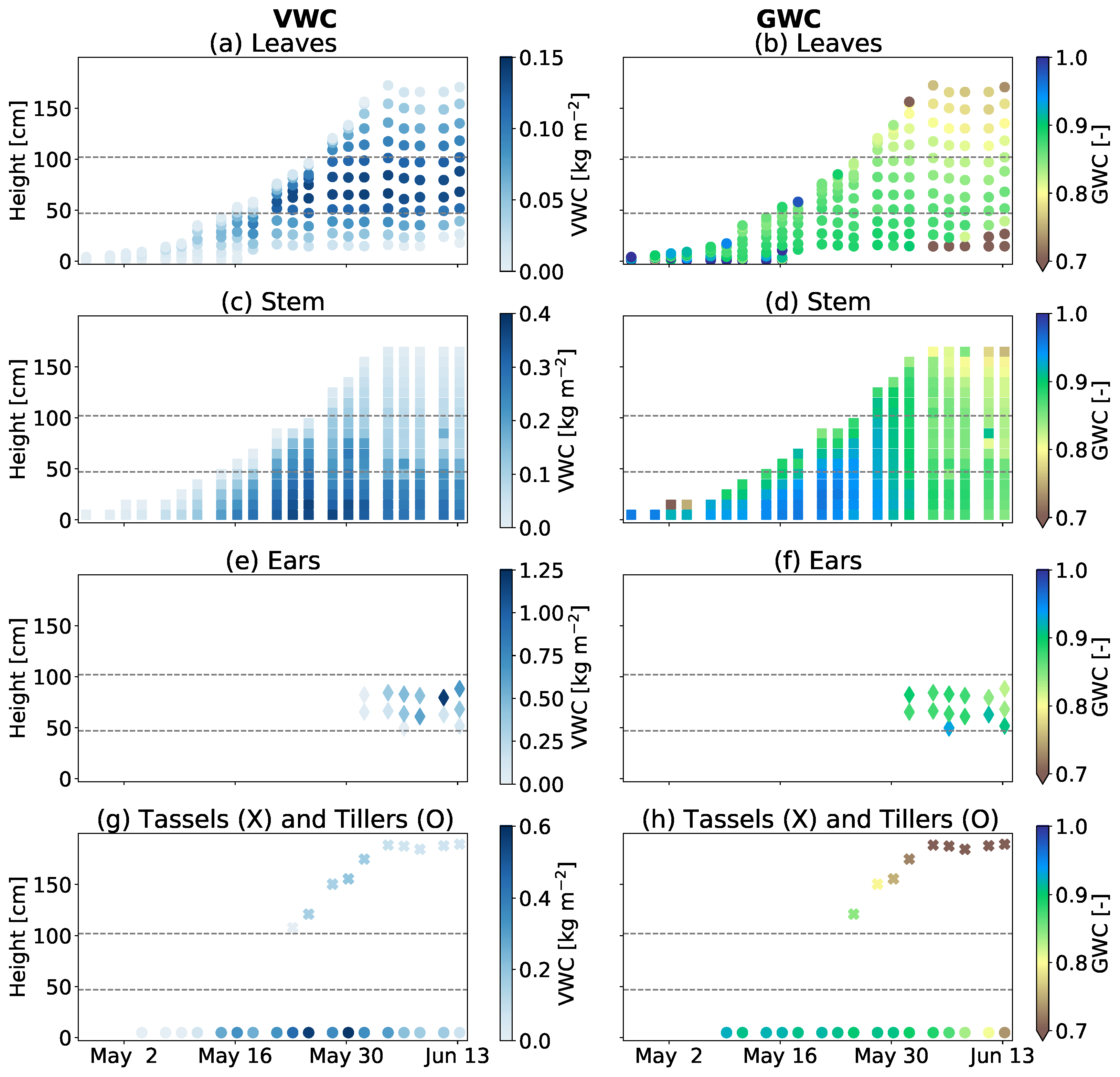
3.1. Seasonal Changes of Internal Vegetation Water Distribution

Figure 1 shows the vertical distribution of VWC (a,c,e,g) and GWC (b,d,f,h) for the different plant constituents and their development during the season. The distribution of VWC is first of all determined by the plant’s structure. Stem water content is, for example, concentrated in the lowest and thickest part of the stem. The first 50 cm of the stems contained 100% (early season) to 60% (late season) of total stem VWC. The four biggest leaves, located between 50 and 100 cm, contained 60% of total leaf VWC in mid- to late season. Attached to these big leaves are the ears, which stored up to 25% of total plant VWC in the late season.
In addition, the aging of the plants has an important effect on the distribution of moisture. The GWC in most of the plant tissue slowly decreases after the first emergence of tassels (25 May), and this drop accelerates after the emergence of ears (1 June; Figure 1b,d,f,h). Leaf senescence starts when the ears separate from the stem (4 June). It starts from the ground up with the lowest leaves, followed by the top leaves from which it progresses down. The largest leaves in the middle of the plant dry out last. Simultaneously, the upper stem dries out. Because this senescence does not occur simultaneously across the vertical profile, variation in moisture across the profile increases from mid- to late season.
Finally, a plant’s moisture content is determined by external factors, such as availability of root zone soil moisture and evaporative demand of the atmosphere, in combination with the hydraulic strategy of the plant. For our corn plants, the effect of these external factors was mainly visible on a sub-daily timescale (see Section 3.2).
Roughly, we can divide the canopy into three vertical layers marked with horizontal dashed lines in Figure 1 and further visualized in Figure 2. The lowest layer, hereafter referred to as layer 1, contains the entire plant in the early season. During the mid- and late season, 60 to 90% of the VWC in the lower layer is stem water, respectively. The amount of water the tillers contained is significant in the mid-season, with 20–25% of total plant VWC in this layer. Compared to the other two layers, layer 1 contains most water until 4 June (Figure 2b).
Layer 2 contains the four biggest leaves, the ears and 50 cm of stem in mid- to late season (Figure 2). The leaf water content in this layer is relatively stable between 21 May and 13 June and is about 0.5 kg m 2 . The relative contributions to total VWC in layer 2 change from 70% leaf and 30% stem on May 18 to 40% leaf and 60% stem on 28 May, just before ear formation, to 25% leaf, 25% stem, and 50% ear on 13 June. From 4 June onward, layer 2 contains most water (Figure 2b).
The upper layer, layer 3, is up to twice as thick as the lower layers and has the lowest water content (Figure 2. It contains the tassels, four leaves and the thinnest part of the stem. Once the layer water content reaches its peak on 30 May, it stays relatively constant (Figure 2b). Despite the decrease of their GWC, leaf and stem VWC remains 0.2 and 0.3 kg m 2 , respectively. This can be explained by the growth of the leaves and stems in this layer and the distribution of water over increasing biomass. Tassel VWC decreased from 0.15 kg m 2 on 25 May to 0.06 kg m 2 on 13 June.

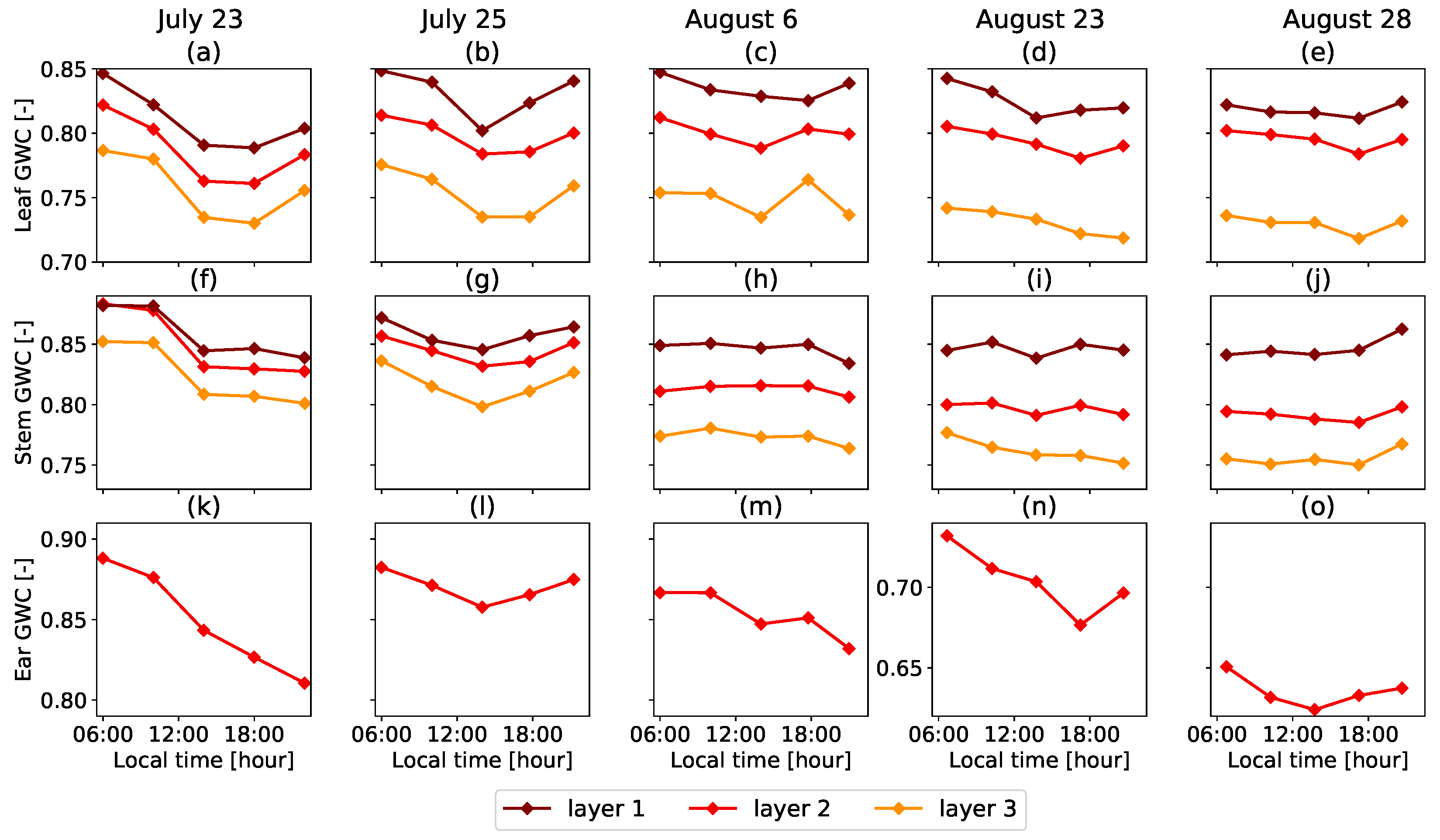
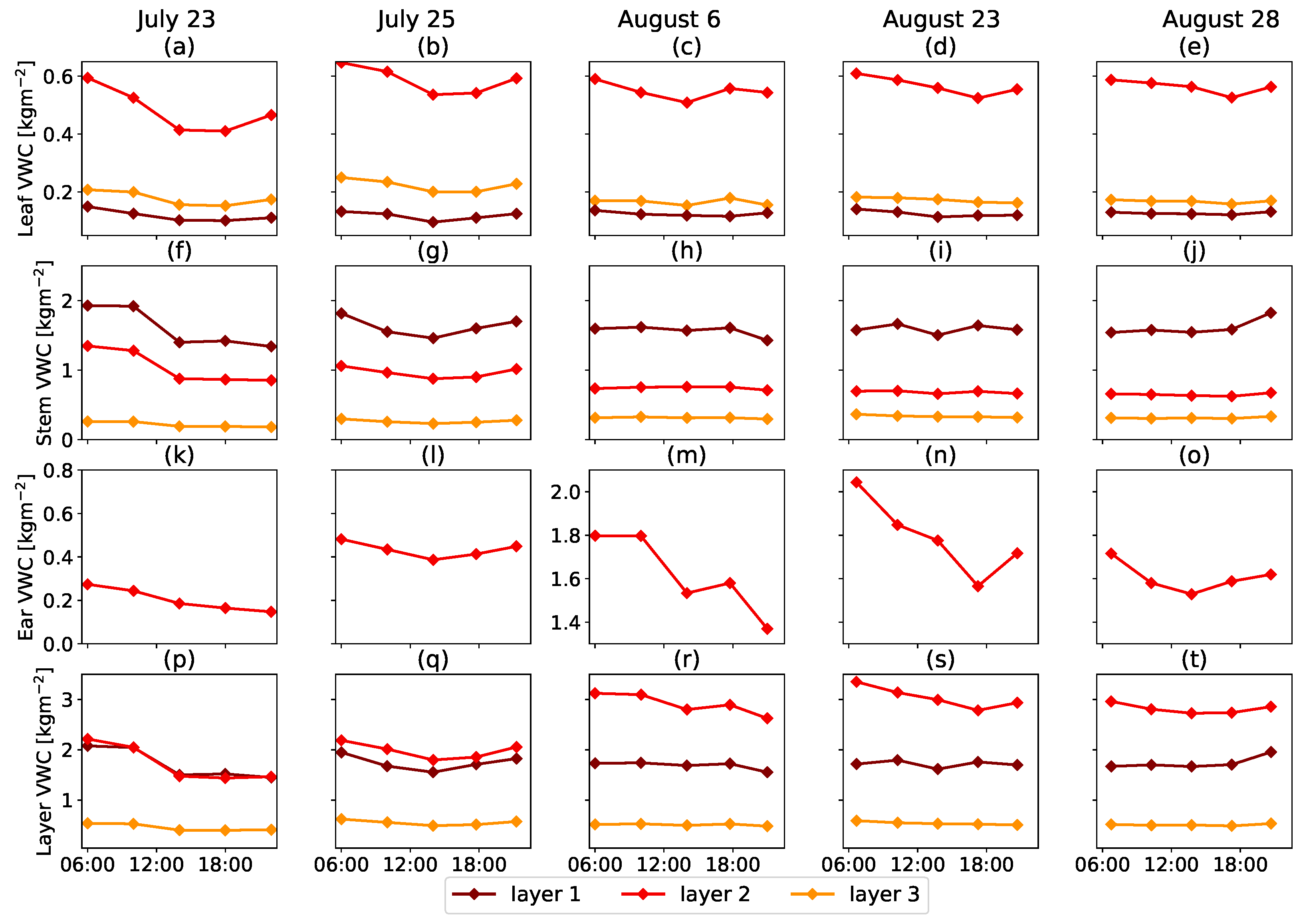
3.2. Sub-Daily Changes of Internal Vegetation Water Distribution

The architecture of a plant also plays a role when it comes to diurnal variations in moisture distribution. It determines which leaves are more or less exposed to solar radiation and wind, the temperature gradient within the canopy and consequently the extent to which the leaves participate in photosynthesis and transpire water [36]. The diurnal patterns in Figure 3 and Figure 4 are the results of sub-daily destructive sampling from field corn in our 2019-campaign in the Netherlands. Figure 3 shows a slightly larger diurnal variability in leaf (a–e) and stem GWC (f–j) in layer 3 on most days, which confirms the role of architecture. However, differences between the layers are minor. Moreover, Figure 4p–t shows that the diurnal variations in layer 3 are limited and that most of the diurnal variation is in the lower two layers.
External factors, such as soil moisture availability and evaporative demand also affect the diurnal variability of VWC. On 23 July, we observed leaf ‘rolling’, a mechanism for drought-stressed corn plants to reduce the leaf area exposed for transpiration [19]. In Figure 3a,f,k, we see that for this day, per constituent, the diurnal GWC pattern of all layers is similar in response to the water deficit. However, leaves, stems and ears respond differently. Where leaves recharge in the evening (a), the water content in the stems stays more or less constant (f), and ear water content still drops (k). From the VWC cycles of 23 July (Figure 4a,f,k), we see that stem VWC dominated layer 1, and, to a lesser extent, also layer 2. The diurnal VWC patterns of layer 1 and 2 are therefore similar (Figure 4p).
Similar to the sweet corn plants (Figure 2; 4 June 2018), we observed a shift in the contribution of the lower two layers to total plant VWC in these field corn plants: after 23 July 2019, layer 2 contains more water than layer 1. In both years, this shift corresponded with the growth of ears. For the diurnal cycles in Figure 4, this means that in July, the diurnal cycles in layer 2 were still dominated by stems and leaves. VWC in layer 2 was lower than (23 July) or equal to (25 July) VWC in layer 1. In August, the ears determined the shape of the diurnal VWC cycle in layer 2 to a great extent.

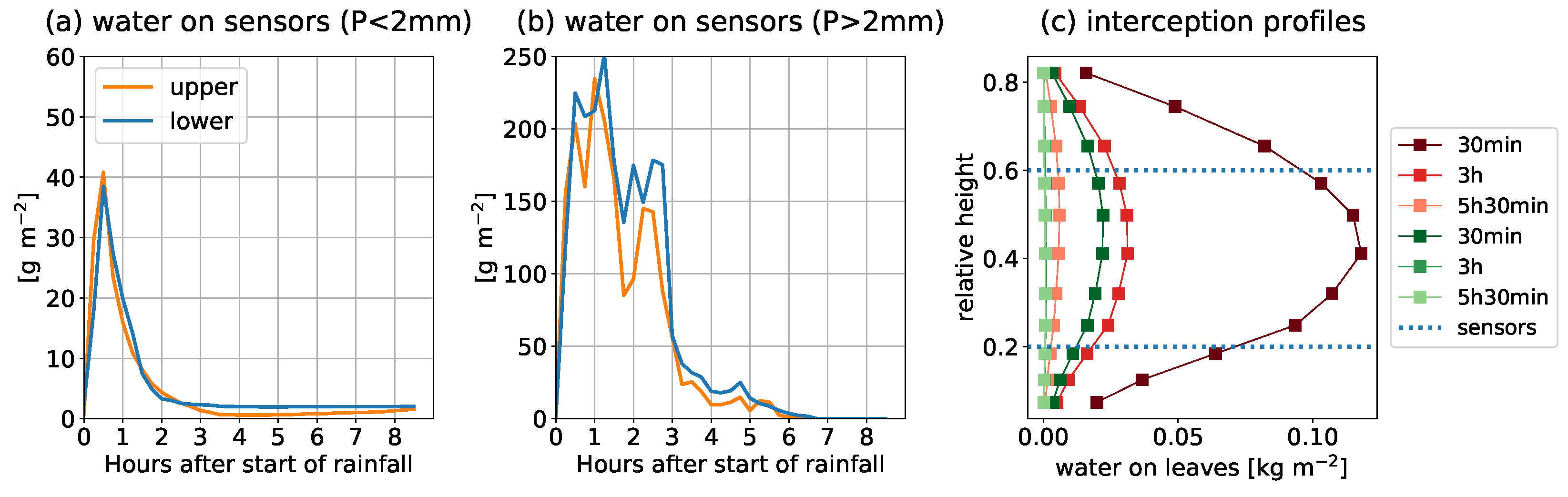
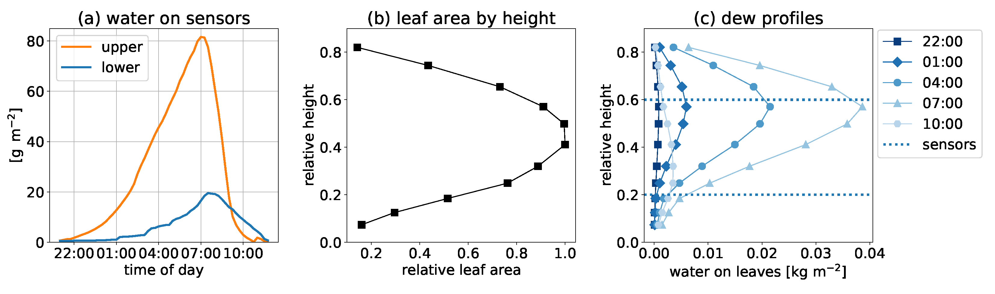
3.3. Distribution of Surface Water: Dew and Rainfall Interception

Figure 5a shows the difference between the mass of dew detected by the upper and lower sensors, Atzema et al. [37] found that 95% of the measured dew could be attributed to dewfall and only 5% to dew-rise, which is the upward soil water vapour flux into the atmosphere during the night. This difference was explained by the fact that a tall and dense crop reduces the amplitude of the daily temperature wave in the non-saturated soil (e.g., [38]) and therefore reduces the dew-rise. However, in the case of a well-watered soil and a stable atmosphere above the canopy, dew-rise will increase as a result of the unstable air between the cooling upper canopy and the heat supply from the soil [37,39,40].
Unlike dew, both sensors detected similar amounts of water during rainfall (Figure 6). This suggests that raindrops penetrated the entire canopy, even during light rain events. The distribution of raindrops through the cascade system of the foliage is a complex process, depending on form, texture and angle of the surface, canopy architecture and density and the number of layers in the cascade [41,42]. However, given the minor differences between the sensor outputs, our estimated interception profiles (Figure 6c) strongly reflect the vertical distribution of leaf area (Figure 5b).

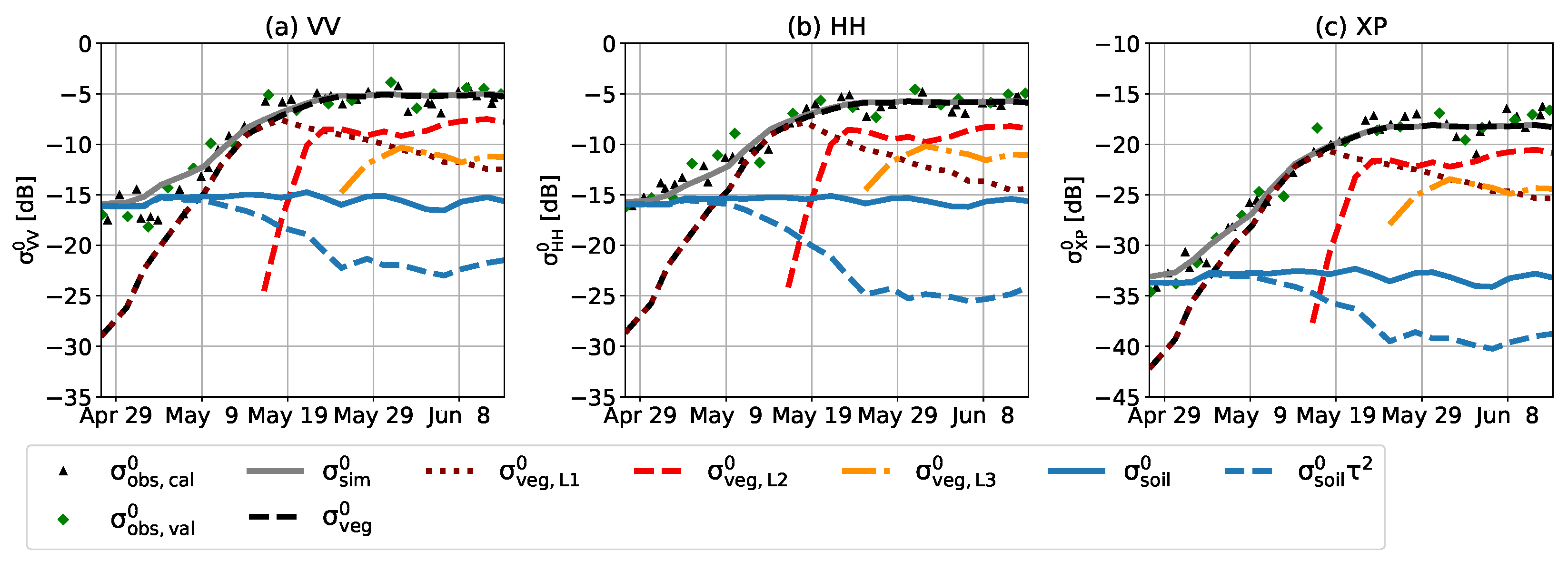
3.4. Multi-Layer WCM: Seasonal Variations

Table 3 shows the WCM calibration results, including the RMSEs of the simulations with respect to the observations as a measure of the model performance.
Figure 7 shows the results from the three-layer WCM, and the observed L-band backscatter ( σ o b s 0 ) for VV (a), HH (b) and cross-pol (c). The contribution from the different layers to total σ v e g 0 changes during the season. In early season, σ v e g 0 equals the contribution from the lowest layer, σ v e g , L 1 0 ; σ v e g , L 1 0 decreases with increasing vegetation growth above this layer. Rapid accumulation of VWC in layer 2 (Figure 2) resulted in a dominant contribution from layer 2 when VWC > 1 kg m 2 (from 23 May onward; Figure 2b and Figure 7), in all polarizations. The simulations showed similar sensitivity of σ v e g 0 to layers 1 (lowest 50 cm) and 3 (upper 100 cm) for VV-pol and cross-pol in the last two weeks of the season. In HH-pol, layer 3 is more dominant in this phase than layer 1. Finally, the simulations showed negligible sensitivity to the attenuated soil moisture signal ( σ s o i l 0 τ 2 ) for co-pols (from VWC > 1 kg m 1 onward) and cross-pols (from VWC > 0.5 kg m 1 onward).
Figure 8 shows the simulated transmissivity ( τ ) decreasing over time and depth in the vegetation layer. The transmissivity in VV-pol (a) and cross-pol (c) is largely similar. For HH-pol, the model found lower transmissivity (and thus higher attenuation). Transmissivity is directly related to Vegetation Optical Depth (VOD; [43]). Consequently, Figure 8 shows that dynamics in a VOD estimate would largely be due to dynamics in layer 1 in the early season and in layer 2 in the late season. This demonstrates the potential value for a multi-layer WCM to interpret VOD estimates.
So far, little research has been conducted on the relative importance of different vertical layers on the backscatter signal. However, we could compare the findings of our modelling study with the results from a recent tomography study by Joerg et al. [44] on field corn. They estimated 3D backscatter profiles from field corn for VV, HH and HV at different frequencies, including L-band, for two growth stages: (1) just before fruit development, and (2) just after fruit development. In our modelling study, we found that the VV and cross-pol scattering contributions from layers 1 and 2 are equally dominant just before fruit development (around 29 May) and more dominant than scattering from layer 3 (Figure 7). In HH-pol, scattering from layer 2 was already most dominant. At this stage, model simulations showed negligible scattering from the ground. Joerg et al. [44] found that at this stage the maximum scattering in all polarizations is centred at ground-level, despite a plant height of 1.9 m. This means scattering from the lowest vegetation layer and the ground. After fruit development (around 13 June), we found dominant scattering from layer 2 in all polarizations. Joerg et al. [44] found that at this stage the maximum return in L-band VV-pol came from scattering at 1/2 to 1/3 of the crop height, which would also be equivalent to layer 2. In addition, they found that the maximum return in HH-pol and HV-pol came from scattering at about 1/4 of the crop height, which would be equivalent to the boundary between layers 1 and 2. This is lower than at VV-pol and also slightly lower than our modelling results.
Compared to previous findings [19], simulations from the WCM used here underestimate the sensitivity to surface soil moisture in the mid- and late season. An important explanation could be that vegetation–ground interactions are not included in the WCM. Previous studies have shown that this term could be considered an important scattering mechanism in corn (e.g., [45,46]). It is expected that considering a vegetation–ground scattering term would increase the sensitivity to surface soil moisture and also might influence the attenuation from the vegetation layer simulated by the WCM.

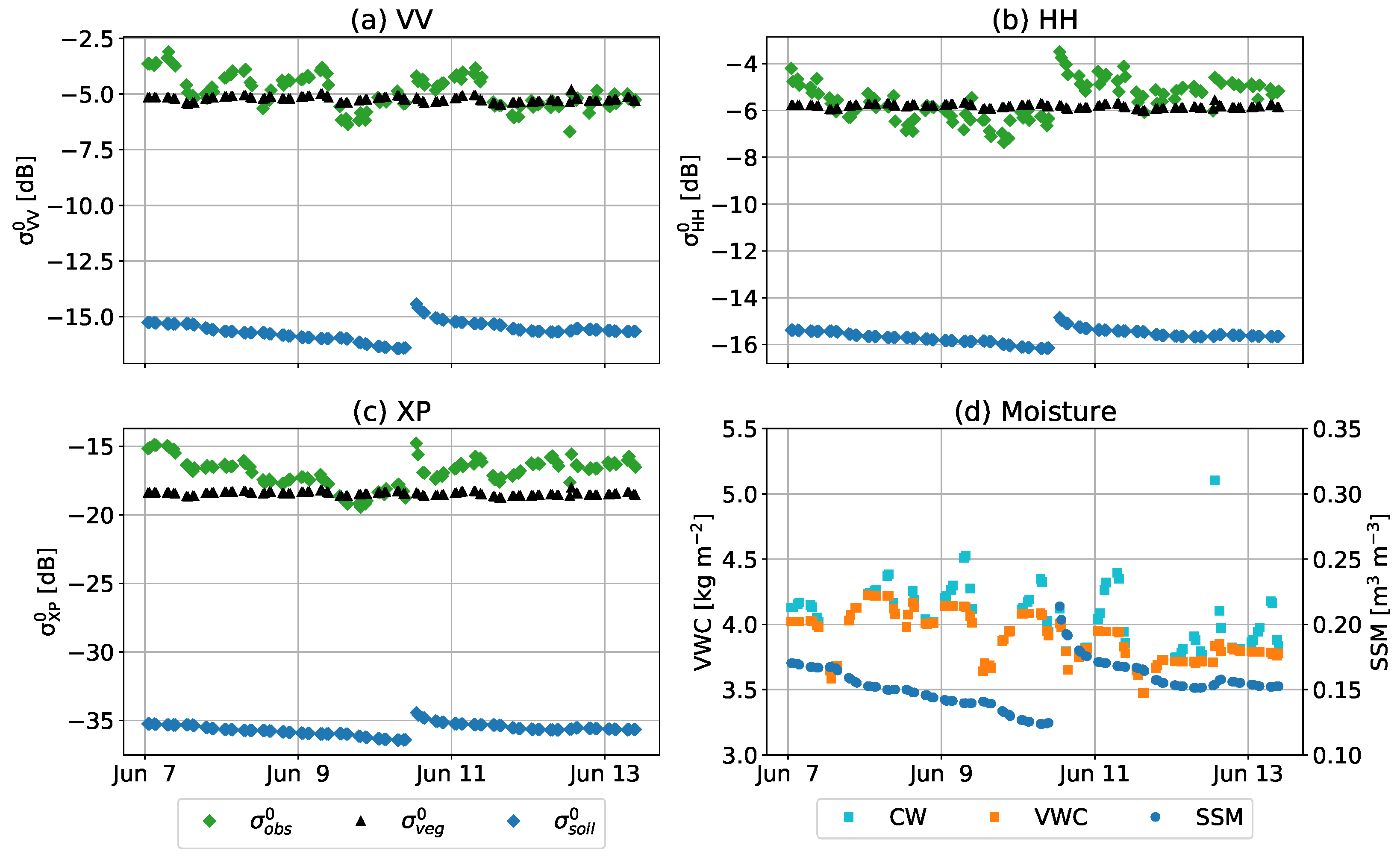
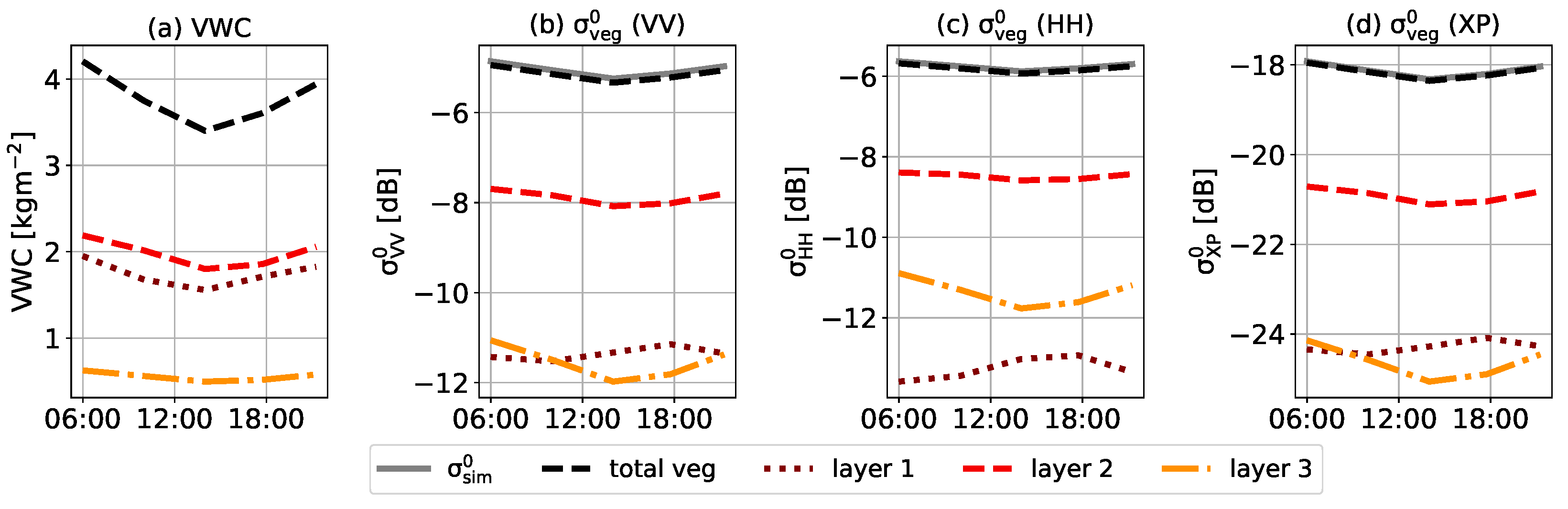
3.5. Multi-Layer WCM: Sub-Daily Variations

The effect of free SCW on variations in layer contributions to σ 0 was estimated by treating SCW as part of the water cloud. In other words, the SCW in a given layer, shown in Figure 9a and Figure 10a, is added to the internal VWC of this layer. The VWC is assumed to be constant in each layer for the model simulations to isolate the effect of SCW. For simplicity, we assumed that parameters C and D, which were calibrated for dry situations, are also valid in these wet situations and that any geometry-related effect accounted for in C and D remains the same regardless of whether the water is VWC or SCW.
Figure 9 and Figure 10 show the effects of dew and rainfall interception on the variations in layer contributions to σ 0 , respectively. Observed σ 0 from dew events could be aggregated and was added to the figure. This was not possible for σ 0 from interception events due to the difference in backscatter acquisition timing since the start of the events. From Figure 9a, it can be seen that nocturnal dew accumulation mainly occurs in layers 2 and 3. When using these estimates as inputs for the WCM, a significant increase in backscatter from layer 3 was found. However, scattering from layer 2 was almost constant or even had a counterbalancing effect (HH) on σ 0 . The latter also holds for layer 1 in all polarizations. The effect of all layers combined was a simulated σ 0 variation of 0.15 dB (VV), 0.10 dB (HH) and 0.16 dB (cross-pol). The fact that dew affects cross-pol and VV-pol more than HH-pol σ 0 is consistent with the observations and previous findings [19]. Both VV- (b) and cross-pol (d) σ o b s 0 show a gradual increase corresponding to dew accumulation and a sharp drop corresponding to dew dissipation. This behaviour was not observed in HH-pol (c). However, the amplitude of the simulated nocturnal ‘cycle’ is much smaller than what is observed in VV-pol and cross-pol. For rainfall interception (Figure 10), we found similar dynamics, except that there was simply more surface water from interception, particularly in layer 2. As a consequence, backscattering from layer 2 had a stronger effect on variation in σ s i m 0 , which was 0.3 dB (VV), 0.2 dB (HH) and 0.3 dB (XP).
Figure 11a shows the layer contribution to diurnal VWC variation for 25 July 2019. Total plant VWC and distribution of moisture between the layers is comparable to that of early June sweet corn in 2018 (Figure 2b). Hence, measurements of this date were used as input for the sweet-corn-calibrated model. It can be seen from Figure 11b–d that σ 0 is dominated by scattering from layer 2 in all polarizations, also with significant contributions from layers 1 and 3. Simulated σ 0 varied with 0.38 dB (b; VV), 0.25 dB (c; HH) and 0.40 dB (d; XP). However, results from [19] suggest that diurnal variations in σ 0 should be in the order of 2 dB as a result of these changes in VWC. Together with differences between observed and simulated σ 0 during dew events (Figure 9), this suggests that sub-daily variations in the WCM simulations are highly underestimated. This is further illustrated in Figure 12. Figure 12a–c shows the observed and simulated VV, HH and XP backscatter variations in the last six days of the season, respectively. Variations in VWC, SCW and SSM are shown in Figure 12d. The sum of SCW and VWC was considered the moisture input for the WCM. Since the difference between simulated σ 0 and σ v e g 0 was negligible at this stage, only σ v e g 0 is depicted. From the analysis in three previous studies [19,20,47], we found that variations in VWC, SCW and SSM affected σ 0 significantly at this stage of the season.
Here, ignoring the vegetation–ground scattering term in the WCM could also play a role. Moreover, high attenuation prevents sub-daily backscattering variations from being captured, which becomes for example apparent from the difference in backscatter contributions from layers 2 and 3 in Figure 9. Comparable amounts of dew were added to layers 2 and 3, but because of much higher attenuation in layer 2 (see Figure 8), we found no nocturnal cycle of σ v e g , L 2 0 compared to a strong nocturnal cycle of σ v e g , L 3 0 . It could be that the WCM simulations overestimated attenuation by the vegetation layer.

4. Conclusions

The aim of this study was to better understand which parts of the vegetation layer control the L-band backscatter dynamics from a corn canopy. Destructive sampling and sensor-based measurements were conducted to illustrate the dynamic vertical distribution of both internal and surface canopy water, respectively, throughout the season. This information was used to define three layers for a multi-layer WCM and simulate the individual layer contributions to total backscatter.
We found that the vertical moisture distribution of VWC is highly dynamic in time. Seasonal changes were mainly affected by the plant’s architecture and age. The bulk of the VWC changed from the lowest 50 cm of the plants, mainly due to stem water storage, to 50–100 cm after ear growth. Diurnal changes were mainly affected by moisture demand and availability. Diurnal dynamics in gravimetric water content were similar across different heights in the canopy. However, the lower parts of the stem and the biggest leaves governed the diurnal VWC cycle together with the ears from mid-season onward. Dew was mainly found in the upper and middle part of the canopy, while rainfall penetrated the entire canopy.
This heterogeneity in moisture distribution means that the contribution of the different vertical layers to total σ v e g 0 varies during the season. Water cloud model simulations showed maximum scattering from the layer with the biggest leaves and the ears in mid-to-late season. The contribution to σ 0 from the lowest 50 cm, which contains most water and mainly from stems, was comparable to the contribution from the top 100 cm for VV- and cross-pol in this phase of the season. HH-pol simulations found more sensitivity to the top 100 cm than to the lowest 50 cm due to slightly higher attenuation. On a sub-daily timescale, variations in σ 0 are sensitive to different parts of the canopy, depending on whether they are caused by dew, interception or fluctuations in VWC. However, variations simulated σ 0 are highly underestimated. This may be explained by overestimated attenuation of the vegetation layers by the WCM or by the importance of the missing vegetation–ground scattering term. Nevertheless, the simulations presented here provide valuable insight into the influence of the changing vertical distribution of moisture in the simplest of radar backscatter models. Sensitivity studies using more sophisticated models that include the ground–vegetation interaction terms are recommended. That said, it is important to note that the WCM is widely used in many applications of microwave remote sensing for vegetation.
This study provides new and unique insights into the contribution of different ’depths’ in a canopy on radar backscatter. Modeling studies, together with other techniques such as tomography, can provide useful insights into the sensitivity of σ 0 to scattering from distinct vertical levels. Our results demonstrate the potential importance of accounting for the vertical moisture distribution when understanding and interpreting backscatter dynamics or products such as vegetation optical depth (VOD).
An important task for future research is to modify the WCM or other electromagnetic models in such a way that they are able to capture sub-daily backscatter dynamics. It is expected that this will improve the estimates of layer contributions to total backscatter. Moreover, considering ground–vegetation scattering should improve the simulated contributions from the different layers. Moreover, future research should focus on the scattering mechanisms related to surface canopy water. The interactions between microwaves with free water on the canopy surfaces (dew, rainfall interception) are still poorly understood. For future field experiments, it is recommended to install a denser network of leaf wetness sensors. This is expected to improve the field-average estimate, and the representation of the uncertainty in the estimates.
To properly understand the potential of using multiple frequencies to determine water content across different heights, it is advised to repeat this experiment with a multi-frequency radar. In addition, shifting the type of vegetation to trees could be interesting. Backscattering from different levels in the canopy may be even more relevant in complex forest systems. A challenge for future research is to understand the backscatter dependence on moisture distribution in forests. The methodology and results presented in this paper contribute to increased interpretation capability of the scattering mechanisms in canopies.

Author Contributions

P.C.V. and S.C.S.-D. were responsible for the conceptualization, methodology, formal analysis, investigation, visualization and writing (original draft preparation); J.J. provided resources (scatterometer data); P.C.V. and S.K. conducted the ground measurements. P.C.V., S.C.S.-D., S.K., V.K. and J.J. contributed to writing (review and editing). All authors have read and agreed to the published version of the manuscript.

Funding

This project was supported by Vidi Grant 14126 from the Dutch Technology Foundation TTW, which is part of The Netherlands Organisation for Scientific Research (NWO), and which is partly funded by the Ministry of Economic Affairs. Support for the field experiment in Florida was obtained from NASA-THP Award #NNX16AQ24G and Center for Remote Sensing, University of Florida.

Acknowledgments

The experiment in 2018 was made possible by infrastructural and technical support from the Agr. and Biol. Eng. Dept. and PSREU at the University of Florida. The authors wish to acknowledge the help from Daniel Preston, Patrick Rush, Eduardo Carrascal, Karin Bremer, and James Boyer and his team in particular. The experiment in 2019 was made possible by infrastructural and technical support from Jacob van den Borne, Paul van Zoggel and their team. Karin Bremer contributed to the design of Figure 2.

Conflicts of Interest

The authors declare no conflict of interest.

References

  1. Kim, Y.; Jackson, T.; Bindlish, R.; Lee, H.; Hong, S. Radar Vegetation Index for Estimating the Vegetation Water Content of Rice and Soybean. IEEE Geosci. Remote Sens. Lett. 2012, 9, 564–568. [Google Scholar] [CrossRef]
  2. Monteith, A.R.; Ulander, L.M.H. Temporal Survey of P- and L-Band Polarimetric Backscatter in Boreal Forests. IEEE J. Sel. Top. Appl. Earth Obs. Remote Sens. 2018, 11, 3564–3577. [Google Scholar] [CrossRef]
  3. Inoue, Y.; Kurosu, T.; Maeno, H.; Uratsuka, S.; Kozu, T.; Dabrowska-Zielinska, K.; Qi, J. Season-long daily measurements of multifrequency (Ka, Ku, X, C, and L) and full-polarization backscatter signatures over paddy rice field and their relationship with biological variables. Remote Sens. Environ. 2002, 81, 194–204. [Google Scholar] [CrossRef]
  4. Brisco, B.; Brown, R.J.; Koehler, J.A.; Sofko, G.J.; McKibben, M.J. The diurnal pattern of microwave backscattering by wheat. Remote Sens. Environ. 1990, 34, 37–47. [Google Scholar] [CrossRef]
  5. Bouman, B.A.M.; Hoekman, D.H. Multi-temporal, multi-frequency radar measurements of agricultural crops during the Agriscatt-88 campaign in The Netherlands. Int. J. Remote Sens. 1993, 14, 1595–1614. [Google Scholar] [CrossRef]
  6. Ferrazzoli, P.; Paloscia, S.; Pampaloni, P.; Schiavon, G.; Solimini, D.; Coppo, P. Sensitivity of microwave measurements to vegetation biomass and soil moisture content: A case study. IEEE Trans. Geosci. Remote Sens. 1992, 30, 750–756. [Google Scholar] [CrossRef]
  7. Narayan, U.; Lakshmi, V.; Njoku, E.G. Retrieval of soil moisture from passive and active L/S band sensor (PALS) observations during the Soil Moisture Experiment in 2002 (SMEX02). Remote Sens. Environ. 2004, 92, 483–496. [Google Scholar] [CrossRef]
  8. Mengen, D.; Brogi, C.; Jakobi, J. The SARSense Campaign: Air-and Space-Borne C-and L-Band SAR for the Analysis of Soil and Plant Parameters in Agriculture. Remote Sens. 2021, 13, 825. [Google Scholar] [CrossRef]
  9. Konings, A.G.; Saatchi, S.S.; Frankenberg, C.; Keller, M.; Leshyk, V.; Anderegg, W.R.L.; Humphrey, V.; Matheny, A.M.; Trugman, A.; Sack, L.; et al. Detecting forest response to droughts with global observations of vegetation water content. Glob. Chang. Biol. 2021, 27, 6005–6024. [Google Scholar] [CrossRef]
  10. Bracaglia, M.; Ferrazzoli, P.; Guerriero, L. A fully polarimetric multiple scattering model for crops. Remote Sens. Environ. 1995, 54, 170–179. [Google Scholar] [CrossRef]
  11. Ulaby, F.T.; Sarabandi, K.; McDonald, K.; Whitt, M.; Dobson, M.C. Michigan microwave canopy scattering model. Int. J. Remote Sens. 1990, 11, 1223–1253. [Google Scholar] [CrossRef]
  12. Link, M.; Jagdhuber, T.; Ferrazzoli, P.; Guerriero, L.; Entekhabi, D. Relationship Between Active and Passive Microwave Signals Over Vegetated Surfaces. IEEE Trans. Geosci. Remote Sens. 2022, 60, 5301715. [Google Scholar] [CrossRef]
  13. Attema, E.P.W.; Ulaby, F.T. Vegetation modeled as a water cloud. Radio Sci. 1978, 13, 357–364. [Google Scholar] [CrossRef]
  14. Ulaby, F.T.; Allen, C.T.; Eger, G.; Kanemasu, E. Relating the microwave backscattering coefficient to leaf area index. Remote Sens. Environ. 1984, 14, 113–133. [Google Scholar] [CrossRef]
  15. Hoekman, D.H. Measurements of the backscatter and attenuation properties of forest stands at X-, C- and L-band. Remote Sens. Environ. 1987, 23, 397–416. [Google Scholar] [CrossRef]
  16. Liu, L.; Shao, Y.; Li, K.; Gong, H. A two layer water cloud model. In Proceedings of the 2012 IEEE International Geoscience and Remote Sensing Symposium, Munich, Germany, 22–27 July 2012; pp. 5840–5843. [Google Scholar] [CrossRef]
  17. Casanova, J.J.; Judge, J.; Jang, M. Modeling Transmission of Microwaves through Dynamic Vegetation. IEEE Trans. Geosci. Remote Sens. 2007, 45, 3145–3149. [Google Scholar] [CrossRef]
  18. Steele-Dunne, S.C.; McNairn, H.; Monsivais-Huertero, A.; Judge, J.; Liu, P.W.; Papathanassiou, K. Radar Remote Sensing of Agricultural Canopies: A Review. IEEE J. Sel. Top. Appl. Earth Obs. Remote Sens. 2017, 10, 2249–2273. [Google Scholar] [CrossRef] [Green Version]
  19. Vermunt, P.C.; Steele-Dunne, S.C.; Khabbazan, S.; Judge, J.; van de Giesen, N.C. Extrapolating continuous vegetation water content to understand sub-daily backscatter variations. Hydrol. Earth Syst. Sci. 2022, 26, 1223–1241. [Google Scholar] [CrossRef]
  20. Vermunt, P.C.; Khabbazan, S.; Steele-Dunne, S.C.; Judge, J.; Monsivais-Huertero, A.; Guerriero, L.; Liu, P.W. Response of Subdaily L-Band Backscatter to Internal and Surface Canopy Water Dynamics. IEEE Trans. Geosci. Remote Sens. 2020, 59, 7322–7337. [Google Scholar] [CrossRef]
  21. McNairn, H.; Jackson, T.J.; Wiseman, G.; Bélair, S.; Berg, A.; Bullock, P.; Colliander, A.; Cosh, M.H.; Kim, S.B.; Magagi, R.; et al. The Soil Moisture Active Passive Validation Experiment 2012 (SMAPVEX12): Prelaunch Calibration and Validation of the SMAP Soil Moisture Algorithms. IEEE Trans. Geosci. Remote Sens. 2015, 53, 2784–2801. [Google Scholar] [CrossRef]
  22. Cosh, M.H.; White, W.A.; Colliander, A.; Jackson, T.J.; Prueger, J.H.; Hornbuckle, B.K.; Hunt, E.R.; McNairn, H.; Powers, J.; Walker, V.A.; et al. Estimating vegetation water content during the Soil Moisture Active Passive Validation Experiment 2016. J. Appl. Remote Sens. 2019, 13, 014516. [Google Scholar] [CrossRef]
  23. Panciera, R.; Walker, J.P.; Jackson, T.J.; Gray, D.A.; Tanase, M.A.; Ryu, D.; Monerris, A.; Yardley, H.; Rüdiger, C.; Wu, X.; et al. The Soil Moisture Active Passive Experiments (SMAPEx): Toward Soil Moisture Retrieval from the SMAP Mission. IEEE Trans. Geosci. Remote Sens. 2014, 52, 490–507. [Google Scholar] [CrossRef]
  24. Judge, J.; Liu, P.W.; Monsiváis-Huertero, A.; Bongiovanni, T.; Chakrabarti, S.; Steele-Dunne, S.C.; Preston, D.; Allen, S.; Bermejo, J.P.; Rush, P.; et al. Impact of vegetation water content information on soil moisture retrievals in agricultural regions: An analysis based on the SMAPVEX16-MicroWEX dataset. Remote Sens. Environ. 2021, 65, 112623. [Google Scholar] [CrossRef]
  25. METER Group, Inc. PHYTOS 31, Dielectric Leaf Wetness Sensor, Product Manual; METER Group, Inc.: Pullman, WA, USA, 2019. [Google Scholar]
  26. Cobos, D.R. Predicting the Amount of Water on the Surface of the LWS Dielectric Leaf Wetness Sensor; Application Note; Decagon Devices, Inc.: Pullman, WA, USA, 2013. [Google Scholar]
  27. Nagarajan, K.; Liu, P.; DeRoo, R.; Judge, J.; Akbar, R.; Rush, P.; Feagle, S.; Preston, D.; Terwilleger, R. Automated L-Band Radar System for Sensing Soil Moisture at High Temporal Resolution. IEEE Geosci. Remote Sens. Lett. 2014, 11, 504–508. [Google Scholar] [CrossRef]
  28. Liu, P.W.; Judge, J.; DeRoo, R.D.; England, A.W.; Bongiovanni, T.; Luke, A. Dominant backscattering mechanisms at L-band during dynamic soil moisture conditions for sandy soils. Remote Sens. Environ. 2016, 178, 104–112. [Google Scholar] [CrossRef]
  29. El Hajj, M.; Baghdadi, N.; Zribi, M.; Belaud, G.; Cheviron, B.; Courault, D.; Charron, F. Soil moisture retrieval over irrigated grassland using X-band SAR data. Remote Sens. Environ. 2016, 176, 202–218. [Google Scholar] [CrossRef] [Green Version]
  30. Li, J.; Wang, S. Using SAR-Derived Vegetation Descriptors in a Water Cloud Model to Improve Soil Moisture Retrieval. Remote Sens. 2018, 10, 1370. [Google Scholar] [CrossRef] [Green Version]
  31. Khabazan, S.; Hosseini, M.; Saradjian, M.R.; Motagh, M.; Magagi, R. Accuracy Assessment of IWCM Soil Moisture Estimation Model in Different Frequency and Polarization Bands. J. Indian Soc. Remote Sens. 2015, 43, 859–865. [Google Scholar] [CrossRef]
  32. Fung, A.K. Microwave Scattering and Emission Models and Their Applications; Artech House: Norwood, MA, USA, 1994. [Google Scholar]
  33. Mironov, V.; Dobson, M.; Kaupp, V.; Komarov, S.; Kleshchenko, V. Generalized refractive mixing dielectric model for moist soils. IEEE Trans. Geosci. Remote Sens. 2004, 42, 773–785. [Google Scholar] [CrossRef]
  34. Gupta, H.V.; Kling, H.; Yilmaz, K.K.; Martinez, G.F. Decomposition of the mean squared error and NSE performance criteria: Implications for improving hydrological modelling. J. Hydrol. 2009, 377, 80–91. [Google Scholar] [CrossRef] [Green Version]
  35. Modanesi, S.; Massari, C.; Gruber, A.; Lievens, H.; Tarpanelli, A.; Morbidelli, R.; De Lannoy, G.J.M. Optimizing a backscatter forward operator using Sentinel-1 data over irrigated land. Hydrol. Earth Syst. Sci. 2021, 25, 6283–6307. [Google Scholar] [CrossRef]
  36. Banerjee, T.; Linn, R. Effect of Vertical Canopy Architecture on Transpiration, Thermoregulation and Carbon Assimilation. Forests 2018, 9, 198. [Google Scholar] [CrossRef] [Green Version]
  37. Atzema, A.J.; Jacobs, A.F.G.; Wartena, L. Moisture distribution within a maize crop due to dew. Neth. J. Agric. Sci. 1990, 38, 117–129. [Google Scholar] [CrossRef]
  38. Yuan, G.; Zhang, L.; Liang, J.; Cao, X.; Guo, Q.; Yang, Z. Impacts of Initial Soil Moisture and Vegetation on the Diurnal Temperature Range in Arid and Semiarid Regions in China. J. Geophys. Res. Atmos. 2017, 122, 11568–11583. [Google Scholar] [CrossRef]
  39. Jacobs, A.F.G.; van Pul, W.A.J.; van Dijken, A. Similarity Moisture Dew Profiles within a Corn Canopy. J. Appl. Meteorol. Climatol. 1990, 29, 1300–1306. [Google Scholar] [CrossRef] [Green Version]
  40. Kabela, E.D.; Hornbuckle, B.K.; Cosh, M.H.; Anderson, M.C.; Gleason, M.L. Dew frequency, duration, amount, and distribution in corn and soybean during SMEX05. Agric. For. Meteorol. 2009, 149, 11–24. [Google Scholar] [CrossRef]
  41. Parker, G. Structure and microclimate of forest canopies. In Forest Canopies; Lowman, M., Nadkarny, N., Eds.; Academic Press: San Diego, CA, USA, 1995; Volume 19, pp. 73–106. [Google Scholar]
  42. De Moraes Frasson, R.P.; Krajewski, W.F. Rainfall interception by maize canopy: Development and application of a process-based model. J. Hydrol. 2013, 489, 246–255. [Google Scholar] [CrossRef]
  43. Frappart, F.; Wigneron, J.P.; Li, X.; Liu, X.; Al-Yaari, A.; Fan, L.; Wang, M.; Moisy, C.; Le Masson, E.; Aoulad Lafkih, Z.; et al. Global Monitoring of the Vegetation Dynamics from the Vegetation Optical Depth (VOD): A Review. Remote Sens. 2020, 12, 2915. [Google Scholar] [CrossRef]
  44. Joerg, H.; Pardini, M.; Hajnsek, I.; Papathanassiou, K.P. Sensitivity of SAR Tomography to the Phenological Cycle of Agricultural Crops at X-, C-, and L-band. IEEE J. Sel. Top. Appl. Earth Obs. Remote Sens. 2018, 11, 3014–3029. [Google Scholar] [CrossRef]
  45. Chauhan, N.; Le Vine, D.; Lang, R. Discrete scatter model for microwave radar and radiometer response to corn: Comparison of theory and data. IEEE Trans. Geosci. Remote Sens. 1994, 32, 416–426. [Google Scholar] [CrossRef]
  46. Monsivais-Huertero, A.; Judge, J. Comparison of Backscattering Models at L-Band for Growing Corn. IEEE Geosci. Remote Sens. Lett. 2011, 8, 24–28. [Google Scholar] [CrossRef]
  47. Khabbazan, S.; Steele-Dunne, S.C.; Vermunt, P.; Judge, J.; Vreugdenhil, M.; Gao, G. The influence of surface canopy water on the relationship between L-band backscatter and biophysical variables in agricultural monitoring. Remote Sens. Environ. 2022, 268, 112789. [Google Scholar] [CrossRef]
Figure 1. Vertical VWC (left) and GWC (right) profiles and their seasonal changes for sweet corn: with leaves (a,b); stems (c,d); ears (e,f); tillers (g); and tassels (g,h). Each marker is the average of 8 plants at a certain height from the ground. Note that the VWC-axes are different among the constituents. The horizontal dashed lines represent the separation of layers for the water cloud model.
Remotesensing 14 03867 g001
Figure 2. Canopy height divided into three layers including LAI (a); total plant VWC divided into three layers (b); and visualisations of the layer division in two different growth stages (c).
Remotesensing 14 03867 g002
Figure 3. Five days of diurnal leaf (ae); stem (fj); and ear (ko); GWC variations in field corn, and the difference between the three vertical layers in the canopy. The sampling was performed five times between sunrise and sunset in the 2019 campaign.
Remotesensing 14 03867 g003
Figure 4. Five days of diurnal leaf (ae); stem (fj); ear (ko); and layer (pt); VWC variations in field corn [kg m 2 ], and the difference between the three vertical layers in the canopy. Layer VWC is the sum of the moisture in all constituents within a certain layer. The sampling was performed five times between sunrise and sunset in the 2019 campaign.
Remotesensing 14 03867 g004
Figure 5. Vertical distribution of dew, with: (a) water detected on upper and lower sensors [g m 2 ] during dew accumulation and dissipation, averaged over 14 dew events; (b) averaged vertical profiles of leaf area for mid-to-late season, with leaf area relative to maximum leaf area and height relative to maximum plant height; and (c) resulting vertical dew profiles changing during the night, including relative heights of sensors.
Remotesensing 14 03867 g005
Figure 6. Vertical distribution of rainfall interception, with the averaged mass of water detected on upper and lower sensors [g m 2 ] during: (a) 6 light rain events (P < 2 mm); and (b) 4 heavy rain events (P > 2 mm) in the period between 1 June and 13 June; and (c) the resulting vertical interception profiles changing during light (green) and heavy (red) rain events, including relative heights of sensors. Note that the data are aggregated. Nocturnal rain events tend to lead to longer periods of canopy wetness, while rainfall interception during the day tends to evaporate rapidly.
Remotesensing 14 03867 g006
Figure 7. Seasonal variations in the contributions of the three different vegetation layers to total vegetation scattering ( σ v e g 0 ), simulated by the 3-layer water cloud model. The different polarizations are separated in: (a) VV; (b) HH; and (c) XP.
Remotesensing 14 03867 g007
Figure 8. Seasonal variations in the transmissivity ( τ ) at different depths of the vegetation layer, simulated by the 3-layer water cloud model. The different polarizations are separated in: (a) VV; (b) HH; and (c) XP.
Remotesensing 14 03867 g008
Figure 9. Averaged dew estimates from 2018 separated by layer (a); and the corresponding nocturnal variations in the layer contributions to total vegetation scattering ( σ v e g 0 ), simulated by the water cloud model and separated by VV (b); HH (c); and cross-polarization (d).
Remotesensing 14 03867 g009
Figure 10. Averaged heavy rainfall interception estimates from 2018 separated by layer (a); and the corresponding variations in the layer contributions to total vegetation scattering ( σ v e g 0 ), simulated by the water cloud model and separated by VV (b); HH (c); and cross-polarization (d).
Remotesensing 14 03867 g010
Figure 11. Diurnal VWC estimates for 25 July 2019 separated by layer (a); and the corresponding diurnal variations in the layer contributions to total vegetation scattering ( σ v e g 0 ), simulated by the water cloud model and separated by VV (b); HH (c); and cross-polarization (d).
Remotesensing 14 03867 g011
Figure 12. Six-day time series with observed backscatter ( σ o b s 0 ), simulated σ v e g 0 from the WCM, and simulated σ s o i l 0 from the IEM, for VV (a); HH (b); and cross-pol (c); moisture variations which served as inputs for the models are shown in (d); with surface soil moisture (SSM) as input for the IEM, VWC and CW, which is the VWC supplemented with dew or rainfall interception and is used as input for the WCM. Sub-daily VWC variations are based on [19].
Remotesensing 14 03867 g012
Table 1. Details of the experimental sites. Measurements from Reusel, the Netherlands (2019), were used for examining sub-daily variations in the vertical distribution of VWC only. For all other analyses, we used data from Citra, Florida (2018).
Citra (2018)Reusel (2019)
Type of cornsweet cornfield corn
Length of season66 days148 days
Plant density7.9 plants m 2 8 plants m 2
Peak dry biomass0.85 kg m 2 2.0 kg m 2
Peak VWC4.5 kg m 2 6.4 kg m 2
Max. height210 cm275 cm
Type of soil>90% sandsandy soil
Climatehumid subtropicaltemperate maritime
Table 2. UF-LARS system specifications.
Parameter UF-LARS
Frequency (GHz) 1.25
3 dB Beamwidth (deg)E-plane14.7
H-plane19.7
Bandwidth (MHz) 300
Antenna type Dual-polarization horn
Range resolution (m)HH/VV/XP8.5/6.2/6.2
Azimuth resolution (m)HH/VV/XP4.7/6.4/4.7
NE σ 0 (dB)HH/VV/XP−23.43/−25.58/−48.12
Error in σ 0 (dB)Systematic1.49
Random0.85
Incidence angle (deg) 40
Platform height (m) 14
Table 3. WCM calibration results.
CDRMSE [dB]
VVHHXPVVHHXPVVHHXP
0.510.390.0260.140.200.131.221.281.24
Publisher’s Note: MDPI stays neutral with regard to jurisdictional claims in published maps and institutional affiliations.

