Abstract
Observations of excited hydroxyl (OH*) emissions are broadly used for inferring information about atmospheric dynamics and composition. We present several analytical approximations for characterizing the excited hydroxyl layer in the Martian atmosphere. They include the OH* number density at the maximum and the height of the peak, along with the relations for assessing different impacts on the OH* layer under night-time conditions. These characteristics are determined by the ambient temperature, atomic oxygen concentration, and their vertical gradients. The derived relations can be used for the analysis of airglow measurements and the interpretation of their variations.
1. Introduction
Hydroxyl molecules in excited states (OH*) produce airglow in visible and near-IR bands. Excited hydroxyl in the vibrationally excited state originates from the reaction of ozone with atomic hydrogen; then, it can be deactivated by collisions with other molecules and atoms, chemically removed by reaction with atomic oxygen, or emit a photon by spontaneous emission. The distribution and abundances of hydroxyl are very sensitive to atmospheric dynamics, thermodynamics, and photochemistry. Therefore, airglow measurements provide a useful tool for studying these processes. In the terrestrial atmosphere, observations of emissions of OH* are broadly used to obtain information about tides [1,2], planetary waves [3,4], gravity waves [5,6,7], and quasi-biennial oscillation [8]. These emissions are also utilized for studying sudden stratospheric warming events [9,10]. Observations of OH* emissions have been used for retrieving temperature trends and variations induced by the solar cycle, e.g., [11,12,13,14,15], and chemical composition in the mesopause region [16,17,18].
Recently, hydroxyl emissions were found in the atmosphere of Venus [19,20,21,22,23] and on Mars [24]. Future observations open the possibility for similar applications of the emissions at these planets (for example, investigations of waves and tides by airglow observations and measurements of atomic oxygen concentrations). Commonly, complex photochemical and general circulation models (i.e., non-linear global with interactively coupled dynamics, chemistry, and radiation) are required for reproducing the behavior of the OH* layer, the main characteristics of which are the altitude, emission intensity, and the shape. When interpretating measurements, it is desirable to establish straightforward relations between these quantities and the ambient temperature, air density, and concentration of minor species involved in photochemical reactions and induced emissions. Since full solutions are complex, it is not easy to assess the impacts of individual processes and interpret the variabilities. Since the conditions differ between planets, we focus on Mars in this paper.
Satellite airglow measurements are not sufficiently precise and result in typical errors in the determination of the layer altitude ~2–3 km. Ground-based observations are restricted to local points and integrated volume emission, which leads to even larger errors in the determination of the altitude (on Earth, the OH* layer is commonly assumed at 87–88 km). In order to study the morphology and variability of the layer, we select the concentration of OH* at the peak, which is directly proportional to the volume emission, and the altitude of the maximum as the characteristics of interest. In the next section, we analytically derive several approximations for these parameters as well as for relative variations of the OH* layer. In Section 3, we present applications of the derived formulae based on the input from the Mars Climate Database (MCD) and determine their validity. Conclusions are given in Section 4.
2. Analytical Formulae Derivation
The list of photochemical reactions pertinent to hydroxyl in the Martian atmosphere, along with the corresponding rates, is given in Table 1.

Table 1.
List of reactions, nomenclature of reaction rates, quenching coefficients, and spontaneous emission coefficients used in the paper.
The table includes the source reaction for vibrationally excited hydroxyl (R1), the reaction of chemical removal (R4), the reactions for collisional deactivation (R5), and spontaneous emission (R6). Reactions R2 and R3 are related to the ozone balance equation, which will be used below. This list omits the reaction of hydroperoxy radicals (HO2) with atomic oxygen because they represent a negligible (or even non-existing) source for the population of vibrationally excited hydroxyl [30,31,32,33,34]. Thus, the starting point of our consideration is the almost complete set of equations for OH*.
Next, we assume that the excited hydroxyl is in a photochemical equilibrium at night [31]; hence, we can write its concentration as a ratio of production to the loss term. This allows us to explicitly express the concentration of excited hydroxyl at all excitation levels (v = 1, …, 9) in the form
where v is the vibrational number; fv are the nascent distributions; r1 and r4 are the reaction rates; and Avv′, Bvv′, Gvv′, and Dvv′ are the quenching coefficients by carbon dioxide, molecular oxygen, molecular nitrogen, and atomic oxygen, respectively. Hereafter, the square brackets denote the number density of a particular chemical constituent. Relation (1) can be simplified by only considering the main processes of production and relaxation, namely, the reaction of ozone with atomic hydrogen, quenching by carbon dioxide, molecular oxygen, and molecular nitrogen:
In (2), we neglected a spontaneous emission and quenching by atomic oxygen because these processes are weak on Mars. For example, the total spontaneous emission coefficients for vibrational levels OHv = 9 and OHv = 1 are E9 = 199.2495 s−1 and E1 = 17.62 s−1, respectively [30]. On the other hand, [CO2] ≥ 1015 cm−3 at 50 km, e.g., [35,36], the collisional removal rates A9 = 9.1 × 10⁻¹¹ cm3 s−1, and A1 = 2.9 × 10⁻¹³ cm3s−1 [29,31,37,38,39] yield the first term in the denominator in (1) exceeding 9 × 10⁴ s−1 and 2.9 × 10² s−1 for the corresponding vibrational numbers. Atomic oxygen concentrations at 50–60 km are around 109–1011 cm−3, e.g., [35,40,41]. Ref. [27] derived for reactive (O + OHv → O2 + H) and non-reactive (O + OHv → OHv′<v + O) quenching rates by atomic oxygen (at T = 160 K) the values 7.7 × 10⁻¹¹ cm3 s−1 and 6 × 10⁻¹¹ cm3 s−1 for v = 9 and 1, respectively. Hence, the corresponding collisional removal rate due to atomic oxygen is less than 8–6 s−1 for all the vibrational numbers and can be neglected.
Following the work of [31], we assume that ozone is in a photochemical equilibrium in the vicinity of the night-time OH* layer. Then, the balance equation for ozone can be represented as
The share of the reaction of ozone with atomic oxygen in total ozone loss is small since, for typical temperatures at 50–60 km (~150 K), the reaction rate r3 (~8.7 × 10⁻¹⁸ cm3 s−1) is about 106 times smaller than r1 (~6.1 × 10⁻¹² cm3 s−1), but the atomic hydrogen number density is smaller than that of atomic oxygen by no more than ~102–103 times in this region [31,35,36,40]. Therefore, the second term on the right-hand side of (3) can be neglected:
The substitution of (4) into the first term in the numerator in (2) gives
Molecular oxygen and molecular nitrogen number densities are linearly proportional to the concentration of carbon dioxide , where M is the air number density, and α, β, and χ are the proportionality coefficients at the heights of the OH* layer, e.g., [35,41]. In the current work, one will find such behavior below in Figure 1a. This allows us to exclude the dependencies on concentrations [O2] and [N2] and re-arrange (5):
where and .
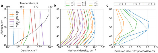
Figure 1.
Night-time zonal mean quantities averaged between 70°N and 90°N and over the period of solar longitudes Ls = 265°–320°: (a) O, O3, H, O2, CO2, N2, T from MCD; (b) OHv = 1,…,9, calculated with (1) (solid lines) and estimated with (7) (dashed lines); (c) volume emissions from (1) and (7) (solid and dashed lines, respectively) for vibrational transitions 1–0 (blue), 2–1 (green), and 2–0 (red).
Writing the numeric value of the reaction rate r2 explicitly and reorganizing (6), we can obtain
where and .
Note that the coefficient ε depends on r2 and, therefore, can vary. For example, refs. [29,31] utilized r2 = 1.2 × 10⁻²⁷ after the work in [42]. The other examples of r2 applied in previous studies include 2.7 × 10⁻³⁴∙3002.4 [40], 1.4 × 10⁻³⁴∙3002.4 [35], and 1.5 × 10⁻³⁴∙3002.4 [43]. Despite the differences, all the studies were in consensus that .
2.1. Peak Concentration of the Excited Hydroxyl Layer and Its Altitude
We now can derive an expression for the peak concentration of the hydroxyl layer OH* and its altitude. For that, we exclude air density M from (7) using the ideal gas law:
where the notation is used, p is pressure, and is the Boltzmann constant.
Differentiating (8) by pressure and equating the result to zero gives the pressure at the local maximum of OH* concentration:
Substituting (9) into (8), we obtain the value of the maximum concentration of the excited hydroxyl:
It is seen from (9) and (10) that the peak concentration of OH* and its height are explicitly determined by vertical profiles of temperature, the concentration of atomic oxygen, and the coefficient , which encompasses photochemical parameters. Note that the derivations above are valid only within a thin layer near the peak of the OH* layer because several assumptions were utilized that are only valid in this region.
2.2. Variations of the Excited Hydroxyl Layer
The hydroxyl layer is extremely variable. Therefore, it is desirable to link its relative variations to those of the observable background quantities. For that, we decompose the atomic oxygen number density, temperature, and air number density into the mean () and deviations (), where the bar denotes an appropriate (spatial, temporal, or both) averaging, and substitute them into (7):
Temperature variations are small, at least on Mars and other planets of the terrestrial group. This allows one to apply the Taylor series expansion to the term with temperature in (11). Cross-multiplying all terms yields
The excited hydroxyl concentration for a given vibrational number can be written in a more compact form:
where the following notations are used:
Hence, relative variations of OH* concentration due to linear parts (RV′) can be expressed in terms of the relative variations of temperature, atomic oxygen, and concentration of air:
The relative variations of the concentration due to second momenta (RV″) are
In the derivation of (14) and (15), namely, in handling the terms with air number density, we assumed that variations of the height of the OH* layer do not exceed the air density scale height. Therefore, the derived equations are only valid when the displacements of the OH* layer from the average altitude do not exceed the air density scale height. In the terrestrial atmosphere, this condition is fulfilled for day-to-day, intra-seasonal, gravity wave-induced variations and for annual cycles at latitudes where height deviations of the OH* layer are relatively small. Similar care should be taken when (14) and (15) are applied on Mars.
3. Calculations and Discussion
In this section, we test the applicability of the derived formulae. They contain photochemical parameters in the most general form. In particular, they assume multi-quantum relaxation for quenching and spontaneous emission processes, where transitions occur from all vibrational levels above to all levels below. To date, not all multi-quantum quenching coefficients for carbon dioxide and molecular nitrogen are known. Only the rates for the so-called collisional cascade quenching [33], where transitions take place to one level below, have been provided in the literature. The most recent update for these coefficients was presented by [28,29] for quenching by carbon dioxide and molecular nitrogen, respectively. We adopted these values in our calculations. Namely, we used the diagonal matrix for Avv′ and Gvv′ for transitions v → v − 1 with values of [28,29] and assigned the non-diagonal terms for other transitions to zero.
The input profiles of O, O3, H, O2, CO2, and N2 concentrations, and temperature, were taken from the Mars Climate Database (MCD), which is based on simulations with the Laboratoire de Météorologie Dynamique General Circulation Model (LMD-GCM) [44,45]. The MCD contains distributions of minor gases in the Martian atmosphere, including ozone [46], which is directly involved in OH* production; water vapor [47], which is the principal source of odd-hydrogens (H, OH, HO2); and variations of other long-lived species (carbon dioxide and molecular nitrogen) involved in quenching processes [48,49].
Figure 1a presents the input profiles of night-time O, O3, H, O2, CO2, and temperature T from the MCD averaged zonally between 70°N and 90°N and over the interval of solar longitudes Ls = 265°–320°. The averaging over this region and time period has been performed in order to provide a colocation with the observations [24]. The results of calculations for [OH*] using the general Formula (1) and approximated by (7) for OHv = 1,…,9 are shown in Figure 1b with solid and dashed lines, correspondingly.
The results illustrate good agreement between OH* concentrations and peak altitudes calculated with the full model (1) and the simplified formula (7). The best agreement occurs near the peaks at ~48–53 km. The differences below and above the maxima can be partially explained by deviations of ozone from photochemical equilibrium in the polar night region, where the ozone lifetime is prolonged under the condition of permanent night and downward transport of atomic oxygen [50].
The vertical separation of the hydroxyl layer depending on vibrational numbers is well-known in Earth’s atmosphere, e.g., [26,51]. It cannot be explained from (9) since v does not depend on p. This is the result of omitting quenching by atomic oxygen in the loss term for excited hydroxyl. The inclusion of this term produces a weak vertical separation by vibrational numbers (solid lines). Vertical distances between layers corresponding to different vibrational numbers are expected to be smaller on Mars than on Earth, as was found by [24]. This is because the atomic oxygen quenching, which is responsible for separation, is comparable with that of molecular oxygen near the Earth mesopause but is negligible compared to the CO2 quenching in the Martian atmosphere.
The increase in excited hydroxyl concentration with decreasing vibrational number was found from observations and modeling for the Earth’s atmosphere [26,28,32,33,51] and from modeling results for the Martian atmosphere [31]. To explain this fact, let us consider Equation (6). Direct population from the reaction of ozone with atomic hydrogen (first term in the numerator) is a slower process than population by quenching from the upper vibrational levels (second term in the numerator). The second term in the numerator (and therefore the whole numerator) increases with a decreasing vibrational number, whereas the denominator can only decrease with a decline in the vibrational number. Thus, the increase in the OH* concentration with a decreasing vibrational number becomes evident.
Volume emission is a measurable quantity that is proportional to the concentration of OH*. We calculated it with the full formula (1) and approximated it by (7) (both assume the photochemical equilibrium of excited hydroxyl) and plotted it in Figure 1c using solid and dashed lines, respectively. The colors indicate the main vibrational transitions: 1–0 (blue), 2–1 (green), and 2–0 (red). The figure shows that the locations of peaks (at ~48–53 km) and the corresponding volume emissions are in good agreement with the observations of [24] in terms of shape and magnitude.
Equations derived in Section 2 provide some predictions and can be applied for analysis in the future, which we illustrate below. The terrestrial OH* airglow layer demonstrates annual and semiannual variations [2,8,52,53]. Similar variations can be expected from the Martian OH* due to seasonal changes in atomic oxygen, air number density, and temperature.
Figure 2 shows time series of night-time one-month sliding averaged values at the peak of the OHv = 2 layer calculated with (1) at middle (40°N) latitudes: (a) the concentration [OHv = 2], (b) the height of the peak, (c) the atomic oxygen concentration, and (d) temperature. It is seen that the concentration and the height of the peak at the northern middle latitude vary seasonally, with the maxim concentrations and lowest height occurring during the first half of the year (Ls ≈ 0°–180°). The amplitude of the annual height variation on Mars is more than 20 km (Figure 2b), which by several times exceeds that near the Earth mesopause (~5–10 km). The figures show a clear anticorrelation between the OHv = 2 number density and the height of the peak, as also follows from (8). Since volume emission is linearly proportional to the hydroxyl concentration, this points to an anticorrelation between the emission and the height of the layer. A similar anticorrelation has also been observed on Earth, e.g., [8,54,55].
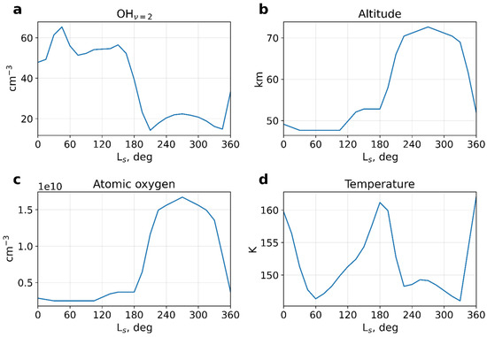
Figure 2.
Night-time mean one-month sliding averaged values at the peak of the OHv = 2 layer calculated with (1) at middle (40° N) latitudes: (a) concentration [OHv = 2], (b) the height of the peak, (c) atomic oxygen concentration, and (d) temperature.
Figure 2a,c demonstrates a correlation between the concentrations of atomic oxygen and excited hydroxyl. This correlation happens between Ls~210° and 340°, where the minor maximum of [OH*] coincides with the maximum of [O]. The correlation between the air number density and the peak altitude is even more robust because the magnitude of seasonal variations of the air density is larger than that of atomic oxygen. The effects of atomic oxygen and air number densities on the OH* layer oppose each other. When the OH* layer is low in summer, the air density is large, while the atomic oxygen concentration is small. The OH* layer moves higher in winter, and the air density decreases, but the atomic oxygen concentration rises. In the Earth’s mesosphere at high and middle latitudes, the behavior of the OH* layer is opposite: high altitude and low emission in summer, but a lower altitude and stronger emission in winter. This is because the main driver for the OH* layer on Earth is atomic oxygen, which is transported downward in winter and upward in summer. On Mars, the layer behavior is additionally determined by air density variations. Seasonal changes in temperature play a minor role in the annual cycle of OH* since it only varies by about 15 K over the year (Figure 2d).
In order to assess the sensitivity of the OH* layer to input parameters, we separately calculated the contributions of relative variations of atomic oxygen, temperature, and air density to variations of [OH*] or to the volume emission rate. We only considered the first half of the year (Ls = 0°–180°), during which displacements of the height of the layer did not exceed the air density scale height (~10 km). Thus, the overbar in (14) and (15) denotes a semiannual averaging, and primes are for deviations from the semiannual mean. As in Figure 2, we only considered night-time values at 40° N, which were smoothed with the one-month moving window averaging.
The results are plotted in Figure 3, with contributions from (14) and (15) shown by solid and dashed lines, respectively. The figure illustrates our notion above that temperature (red lines) plays a minor role in the hydroxyl layer variability. The main contribution comes from variations of atomic oxygen and the ambient air concentration acting in opposite phases. The first peak of [OH*] at Ls~40°–50° (Figure 2a) is primarily determined by the growth of the air number density (blue line) and, to a much lesser degree, by the declining temperature (red line, see also Figure 2d). The secondary peak of [OH*] around Ls~150° is mainly caused by the increase in the atomic oxygen concentration (green line), whereas the declining air density and rising temperature act in the opposite direction. The variations due to second momenta (dashed lines) are much weaker (do not exceed 10%).
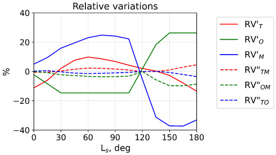
Figure 3.
Relative variations calculated over the first half of the Martian year with (14) (solid lines) and (15) (dashed lines) at 40°N.
4. Conclusions
We presented the derivation of the simplified formulae relating the height of the peak of the excited hydroxyl layer, its displacements, and the strength of emission with values that can be observed in the Martian atmosphere at night-time. The assumptions used in the derivation and relevant for Mars conditions include (1) the photochemical equilibrium of ozone near the peak of the layer and (2) that total quenching by carbon dioxide, molecular oxygen, and molecular nitrogen is greater than quenching by atomic oxygen and spontaneous emission.
Under these approximations, the night-time concentration of OH* near the peak is directly proportional to the concentration of atomic oxygen and pressure and inversely to the power of temperature. Since pressure drops with altitude, the hydroxyl emission, the major part of which is produced in the vicinity of the peak, anticorrelates with the height of the OH* layer.
Calculations using input parameters from the Mars Climate Database demonstrate annual variations of the OH* layer at middle latitude (40°N) resulting from the seasonal cycle of temperature, air number density, and atomic oxygen. We illustrated how relative variations of each of these quantities directly impact the relative variations of the concentration of the hydroxyl layer.
The presented approach and simplified formulae can be applied for the analysis and interpretation of future observations of hydroxyl emission on Mars. Coupled with observations of temperature and atomic oxygen (or ozone), airglow measurements can reveal additional information about the Martian atmosphere’s dynamics and composition.
Finally, we should note that Equations (9) and (10) introduce the possibility of inferring the altitudes of the OH* peak, the concentration at peak, the atomic oxygen concentration at peak, and the ground-state hydroxyl concentration (which is the key constituent for resolving the problem of the Martian (CO2) atmosphere stability due to catalytic recombination [56,57,58]), by surface-based or nadir observations of emissions from two vibrational transitions, accompanied by temperature observations from vibro-rotational transitions following [59].
The strength and advantage of full models are that they seek to most fully encompass processes occurring in a photochemical system. The advantage of an analytical approach is that it allows inferring, under certain conditions and assumptions, simple relations within this system. In this work, we did exactly the latter: derived simplified relations between OH* peak height and density and observable parameters of emission. They can/should motivate the development of future observations and help with interpretations when such observations become available.
Author Contributions
Conceptualization, M.G., D.S.S., A.S.M., G.R.S. and P.H.; methodology, M.G., D.S.S., A.S.M., G.R.S. and P.H.; software, M.G., D.S.S., A.S.M., G.R.S. and P.H.; validation, M.G., D.S.S., A.S.M., G.R.S. and P.H.; formal analysis, M.G., D.S.S., A.S.M., G.R.S. and P.H.; investigation, M.G., D.S.S., A.S.M., G.R.S. and P.H.; writing—original draft preparation, M.G., D.S.S., A.S.M., G.R.S. and P.H.; writing—review and editing, M.G., D.S.S., A.S.M., G.R.S. and P.H.; visualization, M.G., D.S.S., A.S.M., G.R.S. and P.H. All authors have read and agreed to the published version of the manuscript.
Funding
This research was partially funded by Russian Science Foundation grant 20-72-00110.
Data Availability Statement
The MCD data were obtained from the webpage (http://www-mars.lmd.jussieu.fr/, accessed on 12 October 2021). The results of calculations are stored at https://doi.org/10.5281/zenodo.5558814.
Acknowledgments
The authors are grateful to Francois Forget and Jean-Paul Huot for creating the open access Mars Climate Database and to all collaborators of LMD who worked on the database.
Conflicts of Interest
The authors declare no conflict of interest. The funders had no role in the design of the study; in the collection, analyses, or interpretation of data; in the writing of the manuscript, or in the decision to publish the results.
References
- Lopez-Gonzalez, M.J.; Rodríguez, E.; Shepherd, G.G.; Sargoytchev, S.; Shepherd, M.G.; Aushev, V.M.; Brown, S.; García-Comas, M.; Wiens, R.H. Tidal variations of O2 Atmospheric and OH(6-2) airglow and temperature at mid-latitudes from SATI observations. Ann. Geophys. 2005, 23, 3579–3590. [Google Scholar] [CrossRef]
- Xu, J.; Smith, A.K.; Jiang, G.; Gao, H.; Wei, Y.; Mlynczak, M.G.; Russell, J.M., III. Strong longitudinal variations in the OH nightglow. Geophys. Res. Lett. 2010, 37, L21801. [Google Scholar] [CrossRef]
- Buriti, R.A.; Takahashi, H.; Lima, L.M.; Medeiros, A.F. Equatorial planetary waves in the mesosphere observed by airglow periodic oscillations. Adv. Space Res. 2005, 35, 2031–2036. [Google Scholar] [CrossRef]
- Lopez-Gonzalez, M.J.; Rodríguez, E.; García-Comas, M.; Costa, V.; Shepherd, M.G.; Shepherd, G.G.; Aushev, V.M.; Sargoytchev, S. Climatology of planetary wave type oscillations with periods of 2–20 days derived from O2 atmospheric and OH(6-2) airglow observations at mid-latitude with SATI. Ann. Geophys. 2009, 27, 3645–3662. [Google Scholar] [CrossRef]
- Taylor, M.J.; Espy, P.J.; Baker, D.J.; Sica, R.J.; Neal, P.C.; Pendleton, W.R., Jr. Simultaneous intensity, temperature and imaging measurements of short period wave structure in the OH nightglow emission. Planet. Space Sci. 1991, 39, 1171–1188. [Google Scholar] [CrossRef]
- Shepherd, G.G.; Thuillier, G.; Cho, Y.-M.; Duboin, M.-L.; Evans, W.F.J.; Gault, W.A.; Hersom, C.; Kendall, D.J.W.; Lathuillère, C.; Lowe, R.P.; et al. The Wind Imaging Interferometer (WINDII) on the Upper Atmosphere Research Satellite: A 20 year perspective. Rev. Geophys. 2012, 50, RG2007. [Google Scholar] [CrossRef]
- Wachter, P.; Schmidt, C.; Wüst, S.; Bittner, M. Spatial gravity wave characteristics obtained from multiple OH(3-1) airglow temperature time series. J. Atmos. Sol. Terr. Phys. 2015, 135, 192–201. [Google Scholar] [CrossRef]
- Gao, H.; Xu, J.; Wu, Q. Seasonal and QBO variations in the OH nightglow emission observed by TIMED/SABER. J. Geophys. Res. 2010, 115, A06313. [Google Scholar] [CrossRef]
- Shepherd, M.G.; Cho, Y.-M.; Shepherd, G.G.; Ward, W.; Drummond, J.R. Mesospheric temperature and atomic oxygen response during the January 2009 major stratospheric warming. J. Geophys. Res. 2010, 115, A07318. [Google Scholar] [CrossRef]
- Shepherd, M.G.; Meek, C.E.; Hocking, W.K.; Hall, C.M.; Partamies, N.; Sigernes, F.; Manson, A.H.; Ward, W.E. Multi-instrument study of the mesosphere-lower thermosphere dynamics at 80°N during the major SSW in January 2019. J. Atmos. Sol. Terr. Phys. 2020, 210, 105427. [Google Scholar] [CrossRef]
- Bittner, M.; Offermann, D.; Graef, H.-H.; Donner, M.; Hamilton, K. An 18 year time series of OH rotational temperatures and middle atmosphere decadal variations. J. Atmos. Sol. Terr. Phys. 2002, 64, 1147–1166. [Google Scholar] [CrossRef]
- Espy, P.J.; Stegman, J.; Forkman, P.; Murtagh, D. Seasonal variation in the correlation of airglow temperature and emission rate. Geophys. Res. Lett. 2007, 34, L17802. [Google Scholar] [CrossRef]
- Pertsev, N.; Perminov, V. Response of the mesopause airglow to solar activity inferred from measurements at Zvenigorod, Russia. Ann. Geophys. 2008, 26, 1049–1056. [Google Scholar] [CrossRef]
- Dalin, P.; Perminov, V.; Pertsev, N.; Romejko, V. Updated long-term trends in mesopause temperature, airglow emissions, and noctilucent clouds. J. Geophys. Res. 2020, 125, e2019JD030814. [Google Scholar] [CrossRef]
- Perminov, V.I.; Pertsev, N.N.; Dalin, P.A.; Zheleznov, Y.A.; Sukhodoev, V.A.; Orekhov, M.D. Seasonal and Long-Term Changes in the Intensity of O2(b1Σ) and OH(X2Π) Airglow in the Mesopause Region. Geomagn. Aeron. 2021, 61, 589–599. [Google Scholar] [CrossRef]
- Russell, J.P.; Ward, W.E.; Lowe, R.P.; Roble, R.G.; Shepherd, G.G.; Solheim, B. Atomic oxygen profiles (80 to 115 km) derived from Wind Imaging Interferometer/Upper Atmospheric Research Satellite measurements of the hydroxyl and greenline airglow: Local time–latitude dependence. J. Geophys. Res. 2005, 110, D15305. [Google Scholar] [CrossRef]
- Mlynczak, M.G.; Hunt, L.A.; Mast, J.C.; Marshall, B.T.; Russell, J.M., III; Smith, A.K.; Siskind, D.E.; Yee, J.-H.; Mertens, C.J.; Martin-Torres, F.J.; et al. Atomic oxygen in the mesosphere and lower thermosphere derived from SABER: Algorithm theoretical basis and measurement uncertainty. J. Geophys. Res. 2013, 118, 5724–5735. [Google Scholar] [CrossRef]
- Mlynczak, M.G.; Hunt, L.A.; Marshall, B.T.; Mertens, C.J.; Marsh, D.R.; Smith, A.K.; Russell, J.M.; Siskind, D.E.; Gordley, L.L. Atomic hydrogen in the mesopause region derived from SABER: Algorithm theoretical basis, measurement uncertainty, and results. J. Geophys. Res. 2014, 119, 3516–3526. [Google Scholar] [CrossRef]
- Piccioni, G.; Drossart, P.; Zasova, L.; Migliorini, A.; Gérard, J.-C.; Mills, F.P.; Shakun, A.; García Muñoz, A.; Ignatiev, N.; Grassi, D.; et al. First detection of hydroxyl in the atmosphere of Venus. Astron. Astrophys. 2008, 483, L29–L33. [Google Scholar] [CrossRef]
- Gérard, J.-C.; Soret, L.; Saglam, A.; Piccioni, G.; Drossart, P. The distributions of the OH Meinel and O2(a1∆ − X3Σ) nightglow emissions in the Venus mesosphere based on VIRTIS observations. Adv. Space Res. 2010, 45, 1268–1275. [Google Scholar] [CrossRef]
- Soret, L.; Gérard, J.-C.; Piccioni, G.; Drossart, P. Venus OH nightglow distribution based on VIRTIS limb observations from Venus Express. Geophys. Res. Lett. 2010, 37, L06805. [Google Scholar] [CrossRef]
- Migliorini, A.; Piccioni, G.; Cardesín Moinelo, A.; Drossart, P. Hydroxyl airglow on Venus in comparison with Earth. Planet. Space Sci. 2011, 59, 974–980. [Google Scholar] [CrossRef]
- Migliorini, A.; Piccioni, G.; Capaccioni, F.; Filacchione, G.; Tosi, F.; Gérard, J.C. Comparative analysis of airglow emissions in terres-trial planets, observed with VIRTIS-M instruments on board Rosetta and Venus Express. Icarus 2013, 226, 1115–1127. [Google Scholar] [CrossRef]
- Clancy, R.T.; Sandor, B.J.; García-Muñoz, A.; Lefèvre, F.; Smith, M.D.; Wolff, M.J.; Montmessin, F.; Murchie, S.L.; Nair, H. First detection of Mars atmospheric hydroxyl: CRISM Near-IR measurement versus LMD GCM simulation of OH Meinel band emission in the Mars polar winter atmosphere. Icarus 2013, 226, 272–281. [Google Scholar] [CrossRef]
- Burkholder, J.B.; Sander, S.P.; Abbatt, J.; Barker, J.R.; Cappa, C.; Crounse, J.D.; Dibble, T.S.; Huie, R.E.; Kolb, C.E.; Kurylo, M.J.; et al. Chemical Kinetics and Photochemical Data for Use in Atmospheric Studies; Evaluation No. 19; JPL Publication 19-5; Jet Propulsion Laboratory: Pasadena, CA, USA, 2020. Available online: http://jpldataeval.jpl.nasa.gov (accessed on 12 October 2021).
- Adler-Golden, S. Kinetic parameters for OH nightglow modeling consistent with recent laboratory measurements. J. Geophys. Res. 1997, 102, 19969–19976. [Google Scholar] [CrossRef]
- Caridade, P.J.S.B.; Horta, J.-Z.J.; Varandas, A.J.C. Implications of the O + OH reaction in hydroxyl nightglow modeling. Atmos. Chem. Phys. 2013, 13, 1–13. [Google Scholar] [CrossRef]
- Makhlouf, U.B.; Picard, R.H.; Winick, J.R. Photochemical-dynamical modeling of the measured response of airglow to gravity waves. 1. Basic model for OH airglow. J. Geophys. Res. 1995, 100, 11289–11311. [Google Scholar] [CrossRef]
- Krasnopolsky, V.A. Nighttime photochemical model and night airglow on Venus. Planet. Space Sci. 2013, 85, 78–88. [Google Scholar] [CrossRef]
- Xu, J.; Gao, H.; Smith, A.K.; Zhu, Y. Using TIMED/SABER nightglow observations to investigate hydroxyl emission mechanisms in the mesopause region. J. Geophys. Res. 2012, 117, D02301. [Google Scholar] [CrossRef]
- García-Muñoz, A.; McConnell, J.C.; McDade, I.C.; Melo, S.M.L. Airglow on Mars: Some model expectations for the OH Meinel bands and the O2 IR atmospheric band. Icarus 2005, 176, 75–95. [Google Scholar] [CrossRef]
- Llewellyn, E.J.; Long, B.H.; Solheim, B.H. The quenching of OH* in the atmosphere. Planet. Space Sci. 1978, 26, 525–531. [Google Scholar] [CrossRef]
- McDade, I.C.; Llewellyn, E.J. Kinetic parameters related to sources and sinks of vibrationally excited OH in the nightglow. J. Geophys. Res. 1987, 92, 7643–7650. [Google Scholar] [CrossRef]
- Meriwether, J.W., Jr. A review of the photochemistry of selected nightglow emissions from the mesopause. J. Geophys. Res. 1989, 94, 14629–14646. [Google Scholar] [CrossRef]
- Krasnopolsky, V.A.; Lefèvre, F. Chemistry of the atmospheres of Mars, Venus, and Titan. In Comparative Climatology of Terrestrial Planets, 1st ed.; Mackwell, S.J., Simon-Miller, A.A., Eds.; University of Arizona: Tucson, AZ, USA, 2013; pp. 231–275. [Google Scholar] [CrossRef]
- Nair, H.; Allen, M.; Anbar, A.D.; Yung, Y.L.; Clancy, R.T. A Photochemical Model of the Martian Atmosphere. Icarus 1994, 111, 124–150. [Google Scholar] [CrossRef] [PubMed]
- Dodd, J.A.; Lipson, S.J.; Blumberg, W.A.M. Formation and vibrational relaxation of OH(X2Πi, v) by O2 and CO2. J. Chem. Phys. 1991, 95, 5752–5762. [Google Scholar] [CrossRef]
- Chalamala, B.R.; Copeland, R.A. Collision dynamics of OH(X2Π, v = 9). J. Chem. Phys. 1993, 99, 5807–5811. [Google Scholar] [CrossRef]
- Soret, L.; Gérard, J.-C.; Piccioni, G.; Drossart, P. The OH Venus nightglow spectrum: Intensity and vibrational composition from VIRTIS Venus Express observations. Planet. Space Sci. 2012, 73, 387–396. [Google Scholar] [CrossRef][Green Version]
- Krasnopolsky, V.A. Photochemistry of the martian atmosphere: Seasonal, latitudinal, and diurnal variations. Icarus 2006, 185, 153–170. [Google Scholar] [CrossRef]
- Krasnopolsky, V.A. Solar activity variations of thermospheric temperatures on Mars and a problem of CO in the lower atmosphere. Icarus 2010, 207, 638–647. [Google Scholar] [CrossRef]
- Lindner, B.L. Ozone on Mars: The effects of clouds and airborne dust. Planet. Space Sci. 1988, 36, 125–144. [Google Scholar] [CrossRef]
- Lefèvre, F.; Lebonnois, S.; Montmessin, F.; Forget, F. Three-dimensional modeling of ozone on Mars. J. Geophys. Res. 2004, 109, E07004. [Google Scholar] [CrossRef]
- Forget, F.; Hourdin, F.; Fournier, R.; Hourdin, C.; Talagrand, O.; Collins, M.; Lewis, S.R.; Read, P.L.; Huot, J.-P. Improved general circulation models of the Martian atmosphere from the surface to above 80 km. J. Geophys. Res. 1999, 104, 24155–24176. [Google Scholar] [CrossRef]
- Millour, E.; Forget, F.; Spiga, A.; Vals, M.; Zakharov, V.; Montabone, L.; Lefèvre, F.; Montmessin, F.; Chaufray, J.-Y.; López-Valverde, M.A.; et al. The Mars Climate Database (Version 5.3). In Proceedings of the Scientific Workshop: From Mars Express to ExoMars, ESAC, Madrid, Spain, 27–28 February 2018; Available online: https://ui.adsabs.harvard.edu/link_gateway/2018fmee.confE..68M/PUB_PDF (accessed on 12 October 2021).
- Lefèvre, F.; Bertaux, J.-L.; Clancy, R.T.; Encrenaz, T.; Fast, K.; Forget, F.; Lebonnois, S.; Montmessin, F.; Perrier, S. Heterogeneous chemistry in the atmosphere of Mars. Nature 2008, 454, 971–975. [Google Scholar] [CrossRef] [PubMed]
- Navarro, T.; Madeleine, J.-B.; Forget, F.; Spiga, A.; Millour, E.; Montmessin, F.; Määttänen, A. Global climate modeling of the Martian water cycle with improved microphysics and radiatively active water ice clouds. J. Geophys. Res. 2014, 119, 1479–1495. [Google Scholar] [CrossRef]
- Forget, F.; Hourdin, F.; Talagrand, O. CO2 Snowfall on Mars: Simulation with a General Circulation Model. Icarus 1998, 131, 302–316. [Google Scholar] [CrossRef]
- Forget, F.; Millour, E.; Montabone, L.; Lefevre, F. Non condensable gas enrichment and depletion in the Martian polar regions. In Proceedings of the 3rd Workshop Mars Atmosphere: Modeling and Observations, Williamsburg, VA, USA, 10–13 November 2008. [Google Scholar]
- Shaposhnikov, D.S.; Medvedev, A.S.; Rodin, A.V.; Hartogh, P. Seasonal water “pump” in theatmosphere of mars: Vertical transport to the thermosphere. Geophys. Res. Lett. 2019, 46, 4161–4169. [Google Scholar] [CrossRef]
- Swenson, G.R.; Gardner, C.S. Analytical models for the resposes of the mesospheric OH* and Na layers to atmospheric gravity waves. J. Geophys. Res. 1998, 103, 6271–6294. [Google Scholar] [CrossRef]
- Liu, G.; Shepherd, G.G.; Roble, R.G. Seasonal variations of the nighttime O(1S) and OH airglow emission rates at mid-to-high latitudes in the context of the large-scale circulation. J. Geophys. Res. 2008, 113, A06302. [Google Scholar] [CrossRef]
- Marsh, D.R.; Smith, A.K.; Mlynczak, M.G.; Russell, J.M., III. SABER observations of the OH Meinel airglow variability near the mesopause. J. Geophys. Res. 2006, 111, A10S05. [Google Scholar] [CrossRef]
- Liu, G.; Shepherd, G.G. An empirical model for the altitude of the OH nightglow emission. Geophys. Res. Lett. 2006, 33, L09805. [Google Scholar] [CrossRef]
- Mulligan, F.G.; Dyrland, M.E.; Sigernes, F.; Deehr, C.S. Inferring hydroxyl layer peak heights from ground-based measurements of OH(6–2) band integrated emission rate at Longyearbyen (78°N, 16°E). Ann. Geophys. 2009, 27, 4197–4205. [Google Scholar] [CrossRef][Green Version]
- McElroy, M.B.; Donahue, T.M. Stability of the Martian Atmosphere. Science 1972, 177, 986–988. [Google Scholar] [CrossRef] [PubMed]
- Parkinson, T.D.; Hunten, D.M. Spectroscopy and aeronomy of O2 on Mars. J. Atmos. Sci. 1972, 29, 1380–1390. [Google Scholar] [CrossRef]
- Olsen, K.S.; Lefèvre, F.; Montmessin, F.; Fedorova, A.A.; Trokhimovskiy, A.; Baggio, L.; Korablev, O.; Alday, J.; Wilson, C.F.; Forget, F.; et al. The vertical structure of CO in the Martian atmosphere from the ExoMars Trace Gas Orbiter. Nat. Geosci. 2021, 14, 67–71. [Google Scholar] [CrossRef]
- Conway, S. Methods for Deriving Temperature Profiles of Mars from OH Meinel Airglow Observations. Ph.D. Thesis, York University, Toronto, ON, Canada, March 2012. [Google Scholar]
Publisher’s Note: MDPI stays neutral with regard to jurisdictional claims in published maps and institutional affiliations. |
© 2022 by the authors. Licensee MDPI, Basel, Switzerland. This article is an open access article distributed under the terms and conditions of the Creative Commons Attribution (CC BY) license (https://creativecommons.org/licenses/by/4.0/).