Mapping Forest Stability within Major Biomes Using Canopy Indices Derived from MODIS Time Series

Abstract

Deforestation and forest degradation from human land use, including primary forest loss, are of growing concern. The conservation of old-growth and other forests with important environmental values is central to many international initiatives aimed at protecting biodiversity, mitigating climate change impacts, and supporting sustainable livelihoods. Current remote-sensing products largely focus on deforestation rather than forest degradation and are dependent on machine learning, calibrated with extensive field measurements. To help address this, we developed a novel approach for mapping forest ecosystem stability, defined in terms of constancy, which is a key characteristic of long-undisturbed (including primary) forests. Our approach categorizes forests into stability classes based on satellite-data time series related to plant water–carbon relationships. Specifically, we used long-term dynamics of the fraction of photosynthetically active radiation intercepted by the canopy (fPAR) and shortwave infrared water stress index (SIWSI) derived from the Moderate Resolution Imaging Spectroradiometer (MODIS) for the period 2003–2018. We calculated a set of variables from annual time series of fPAR and SIWSI for representative forest regions at opposite ends of Earth’s climatic and latitudinal gradients: boreal forests of Siberia (southern taiga, Russia) and tropical rainforests of the Amazon basin (Kayapó territory, Brazil). Independent validation drew upon high-resolution Landsat imagery and forest cover change data. The results indicate that the proposed approach is accurate and applicable across forest biomes and, thereby, provides a timely and transferrable method to aid in the identification and conservation of stable forests. Information on the location of less stable forests is equally relevant for ecological restoration, reforestation, and proforestation activities.

1. Introduction

Deforestation and forest degradation from anthropogenic impacts are now understood as a matter of global environmental concern [1]. Primary forests, which represent the most natural end of the forest ecological condition gradient, are under particular threat. According to the Food and Agriculture Organization (FAO) and the International Union for Conservation of Nature (IUCN), primary forests are defined as naturally regenerated forests of native species where there are no clearly visible indications of modern human land use activities and ecological processes dominate [2,3]. Primary forests typically have larger ecosystem carbon stocks, provide habitat for a wider range of species, yield cleaner water, and are overall more stable and resilient to external stressor, as well as have higher natural adaptive capacity, compared to degraded and secondary growth forest [4,5,6,7,8,9,10,11]. Therefore, the degradation of primary forests due to human land use and related impacts can result in loss of valued ecosystem services for climate change mitigation, biodiversity conservation, and sustainable livelihoods.

To date, deforestation (i.e., forest clearing) has been successfully monitored by using remote-sensing approaches [12,13,14]. On the other hand, quantifying forest degradation presents a major challenge because it typically results in subtler changes in structure, composition, and function of forest ecosystems [15,16]. The main approaches to characterize forest degradation include detection of changes in tree canopy cover and quantification of losses in above ground biomass [4,17,18,19,20]. Although high-resolution forest cover maps are now available globally (see Reference [21], for example) and provide spatial estimates of key forest canopy structural characteristics, a number of problems in their application to mapping forest degradation persist. First, these spatial layers are derived from machine learning by using satellite data trained on extensive networks of field-based measurements, which are expensive to obtain and represent a geographically limited sample of forest conditions. Secondly, wet tropical forests that are logged or cleared can quickly recover a closed canopy through pioneer and secondary successional growth. Thus, satellite-based sensors and modeled forest cover data are often unable to distinguish regrown canopies from those of primary forest [22]. A different issue arises in the temperate and boreal biomes since these forests are naturally subject to recurrent disturbances, including wildfire and insect outbreaks [23]. As a result, forest landscapes can comprise a rich mosaic of stands in different successional stages [24]. Consequently, it is difficult to differentiate between forests that have been disturbed by human land use, including logging from those that are the result of natural disturbance regimes [25]. The challenge here is to first delineate between undisturbed, degraded, and fully disturbed forests and then to attribute the latter to natural or human-induced processes.

Another issue when mapping forest loss and degradation is related to the spatial scale of analysis. Internationally recognized and used definitions of forest [3] are based on minimalistic structural criteria (land area ≥ 0.5 ha, tree crown cover ≥ 10%, and canopy height at maturity ≥ 5 m), and recent data products are available at 30 m, making use of the Landsat satellites. However, naturally regenerating wet tropical forests, as distinct from forest plantations (i.e., tree crops), represent dynamic landscape-scale phenomena reflecting multiple physical, ecological, and biological processes [26] and more typically have a canopy density ≥ 30% and tree height ≥ 20 m [27]. The landscape perspective is equally important in the boreal biome given the spatially varying patterning of forest ecosystem types and seral stages as the result of heterogeneity in topography, soil substrate, and natural disturbance regimes [28,29].

Here, we propose that the ecological concept of stability provides a useful theoretical framework for mapping forest degradation in both wet tropical and boreal forest biomes. Stability can be defined in terms of three properties: constancy (i.e., resistance), resilience, and persistence [30]. When assessed over an appropriate period of time, a forest with a high level of ecosystem stability will have a constant canopy condition (i.e., be resistant), recover to the reference state after a temporary disturbance (i.e., be resilient), and persist in the landscape through multiple disturbance cycles (i.e., be persistent). While constancy is the most relevant of these properties in the wet tropics, resilience and persistence also play an important role in the boreal ecosystems due to the inherit complexity of forest landscapes caused by mosaicked patchwork of seral stages following natural disturbances. However, given the natural extent of old-growth forests in the boreal biome [23], the constancy property of stability is still a pertinent feature to characterize undisturbed areas since long-lived trees respond slowly to transient changes in the system and maintain stability via dynamic equilibrium within defined bounds [31,32]. It follows that mapping stability requires the use of time-series data rather than a single ‘snapshot’ in time. Furthermore, the time-series analysis should be undertaken at a spatial resolution commensurate with the landscape-scale characteristics of tropical and boreal forest ecosystems. We also suggest that the need for extensive field data can be avoided by using metrics based on readily available satellite data which have a well-established ecological interpretation.

Here we examine the constancy property of stability in tropical and boreal forests by using a novel approach based on remote-sensing indices that are known to be correlated with ecophysiological processes driving plant water–carbon relationships [33], which, in turn, are related to vegetation structure [34]. Specifically, we use the fraction of photosynthetically active radiation intercepted by the sunlit canopy (fPAR) [35,36] and the shortwave infrared water stress index (SIWSI) derived from the Moderate Resolution Imaging Spectroradiometer (MODIS). Moreover, fPAR is related to both vegetation structure (leaf area and orientation) and primary productivity [37,38], and SIWSI is a robust indicator of plant water content in fine tissues [39], particularly in green leaves [40]. SIWSI time series can therefore be indicative of water stress dynamics and the microclimate buffering capacity of structurally intact forest canopies. The latter determines the extent to which below-canopy climatic conditions deviate from the climate outside forests. We developed a set of variables calculated from annual time series of fPAR and SIWSI for two representative forested regions at opposite ends of Earth’s climatic and latitudinal gradient: the boreal forests of Siberia (southern taiga, Russia) and tropical rainforests of the Amazon basin (Kayapó territory, Brazil). We validated our results by comparing them with several independent data sources (see Section 2.3 for more information) to ensure that our mapped stability categories equated to known distributions of disturbance and intact forest canopies (noting the inherent limitation of validating low stability forests, for which our method provides a first estimate).

2. Materials and Methods

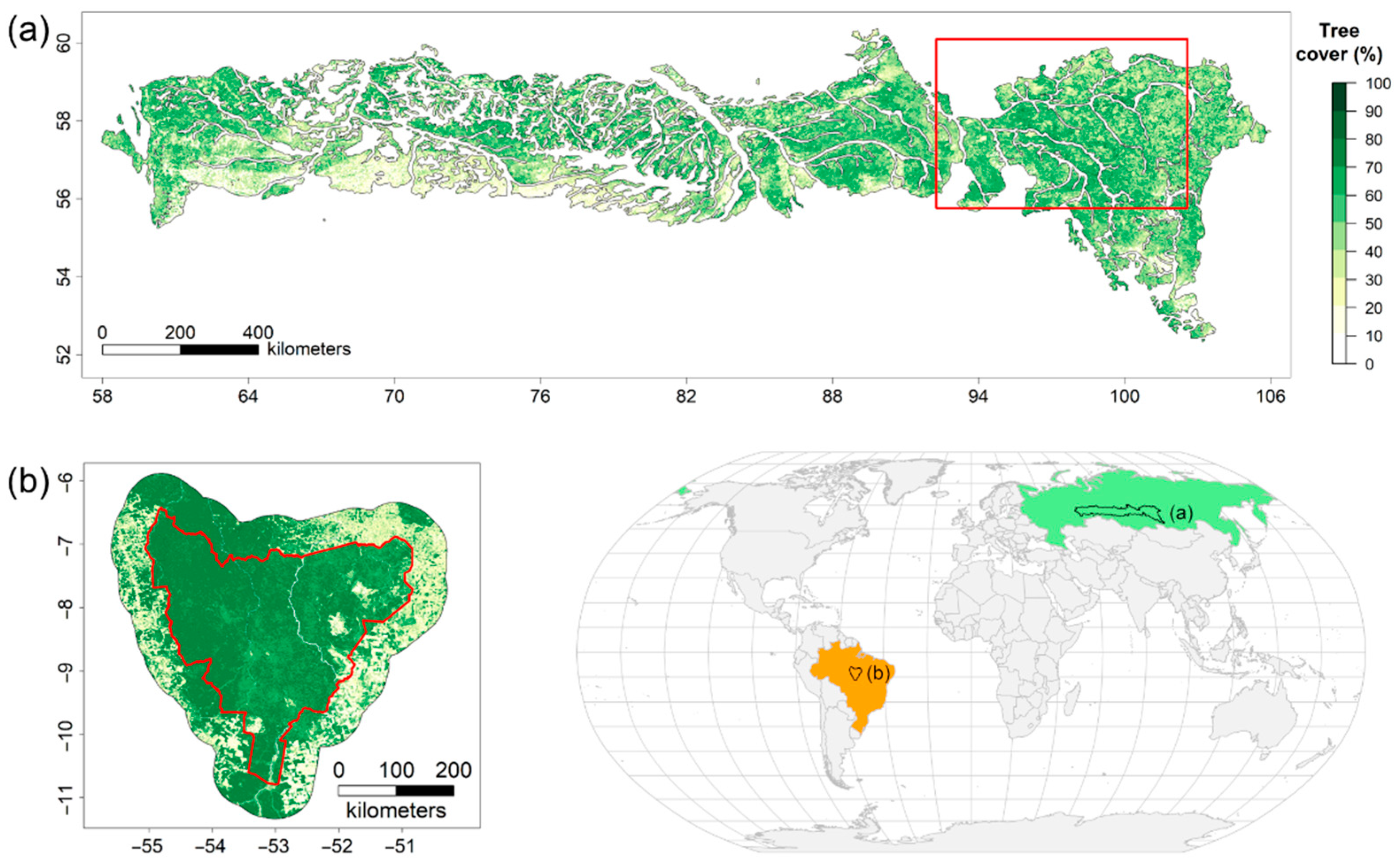
2.1. Study Regions

We focused on two case study regions in contrasting forest biomes from different continents: the boreal taiga (Eurasia) and the tropical rainforest (South America). Within these, we targeted the southern taiga ecoregion of Siberia (Russia) and the Kayapó indigenous territory within the Amazon basin (Brazil) (Figure 1). These regions are representative of the aforementioned biomes and contain the full spectrum of forest ecosystem conditions: significant areas of primary forests [3] and intact forest landscapes still exist [41], along with forests that are heavily managed for commodity production and forests cleared for agricultural use. Many areas within both regions have been heavily exploited since the mid-20th century, resulting in substantial fragmentation and degradation. Fires and intensifying industrial logging are major threats to the sustainability of these forests, with the majority of fire ignitions in both regions caused by humans [42,43]. Moreover, human activities are radically altering their natural fire dynamics owing to altered fuel loads, desiccation, and flammability within or in proximity to human-altered landscapes [44,45,46,47,48,49,50].

Climate differs markedly between these regions, particularly with respect to thermal regime, degree of seasonality and growing season length (Supplementary Table S1). Extreme continentality is characteristic of the southern taiga, with large daily and seasonal ranges of temperature, solar radiation, and day length. These fluctuations are far smaller in tropical forests. Such differences have profound implications for forest composition, structure, function, and dynamics.

For the southern taiga, we defined the study area based on ecoregion boundaries to facilitate the identification of forest stability classes relative to a broad ecosystem type. In this way, we controlled for the existing differences in vegetation structure and floristics (e.g., dominant species, maximum canopy height and density) across boreal Russia, since these are largely influenced by the predominant physical environmental conditions. We used an ecoregion division for Russia from previous studies [51,52] that includes—from west to east—the administrative territories of Sverdlovsk, Tyumen, Omsk, Novosibirsk and Tomsk oblasts, Krasnoyarsk krai, and Irkutsk oblast. For the Amazon rainforest, the study region coincided with the Kayapó indigenous territory in the Brazilian states of Pará and Mato Grosso. This is an extensive area of largely primary tropical forest. We added a buffer zone of 60 km around the perimeter of the Kayapó territory to include areas that have been disturbed, degraded, and cleared by modern land use. The total study area comprised 120 million ha and 22 million ha of southern taiga and tropical forest, respectively.

2.2. Data Analysis

2.2.1. Input Parameters

For each region, we used 16-year monthly time series (2003–2018) of (i) the fraction of photosynthetically active radiation intercepted by sunlit vegetation canopy (fPAR) and (ii) the shortwave infrared water stress index (SIWSI). Both metrics were obtained from MODIS satellite imagery at ~500 m (463 m) spatial resolution. Moreover, fPAR represents the fraction of incoming solar radiation between 400 and 700 nm absorbed by plant canopies and was taken from the MCD15A3H v6 Leaf Area Index/FPAR 4-day L4 global product [53]. SIWSI was derived from the near infrared (NIR; 841–876 nm) and the shortwave infrared (SWIR; 1628–1652 nm) bands, using the MOD09A1 v6 Terra Surface Reflectance 8-Day Global product, as follows [54]:

SIWSI = (SWIR − NIR)/(SWIR + NIR)

(1)

For both products, we identified pixels that were affected by cloud contamination or sensor errors, using quality flags provided with the MODIS imagery. Particularly, we excluded pixels that contained high aerosol levels (bit 3), cirrus (bit 4), clouds (bit 5), or cloud shadows (bit 6). We then generated a mean monthly time series of fPAR and SIWSI from 2003 to 2018. We limited our analysis to June–August, which corresponds to the growing season in the southern taiga and the dry season in the Amazon rainforest. For the southern taiga, this procedure was useful to minimize variation related to seasonal changes in ground cover (i.e., snow) and vegetation greenness (i.e., phenology of deciduous trees). In contrast, the natural variation in satellite-derived vegetation indices over tropical rainforests is relatively small throughout the year due to the presence of a dense evergreen tree canopy. Therefore, inter-annual changes in forest greenness and canopy water content were expected to be particularly pronounced during the dry season (especially July and August) in the Amazon rainforest [55]. Finally, we masked out non-vegetative pixels corresponding to water, permanent wetlands, barren land, and urban areas, as well as croplands and crop-natural vegetation mosaics, using the MCD12Q1 Land Cover Type product corresponding to the year 2018 [56].

To assess forest-ecosystem stability, per-pixel metrics were generated from image stacks of mean June–August fPAR and SIWSI values over the period 2003–2018. For each variable, we first calculated the 16-year mean time-series value (fPAR_mean and SIWSI_mean) and its coefficient of variation (fPAR_CV and SIWSI_CV). These metrics provide information on the long-term average canopy greenness (fPAR), vegetation water stress (SIWSI), and their inter-annual variability (for mean and CV, respectively). The minimum seasonal fPAR (fPAR_min) and maximum seasonal SIWSI (SIWSI_max) values of the 16-year time series were calculated to provide information about the poorest (e.g., most water-stressed) vegetation condition attained by each pixel over the study period. In addition, we calculated linear annual trends (slopes) of seasonal fPAR and SIWSI for each pixel, using nonparametric Theil–Sen regression models. Slopes were obtained in order to characterize linear changes in vegetation status. Here, we focused on absolute slope values, which were indicative of the presence or absence of temporal trends but not of the direction of the trend (i.e., ‘greening’ or ‘browning’). We considered a change in slope of both metrics as the direct result of forest disturbance due to either natural ecological processes, such as insect outbreaks, and/or human disturbances, such as logging and clearing. During the observation period, large positive slopes indicate forest succession following a prior disturbance, while large negative slopes indicate a disturbance during the time series. Areas with essentially no change were considered as those lacking alteration to surface features at the MODIS pixel scale (ca. 500 m).

2.2.2. k-Means Clustering of Pixels

Pixels with similar fPAR and SIWSI metric values were categorized into homogeneous classes by means of k-means clustering, which is an unsupervised algorithm that forms groups based on cluster centers. The use of an unsupervised algorithm has two main advantages compared to other approaches. First, it eliminates the need for extensive field-based observations to serve as training data for calibrating the remotely sensed metrics against surface features of interest. Second, this method is independent of particular environmental and forest characteristics, and, hence, it can be applied to any forested region, allowing for the application of a common approach to both boreal and tropical biomes. On the other hand, unsupervised algorithms require that great care is taken in selecting an appropriate area of interest and remotely sensed metrics to define the clusters since vague or inappropriate spectral grouping may not correspond to classes of interest. In addition, it demands a good knowledge of the ecosystems under evaluation to interpret unique classes produced during the classification, especially when they represent processes and not features on the ground [57].

All input variables underwent a two-step transformation prior to clustering. First, we tested whether the values of each variable were normally distributed through Shapiro–Wilk tests. If needed, the data were transformed to a new scale that better conformed to a normal distribution. The logarithmic transformation was used on all variables, except for slopes, where a cubic root transformation was applied. We then standardized the data to a uniform scale of 0–100, thereby allowing each variable to have the same weight in the clustering procedure. These procedures were performed at a biome scale for each region separately.

For the application of k-means, we defined 30 clusters (k = 30) that captured the natural variability at regional scales based on the previously defined parameters derived from fPAR and SIWSI time series, i.e., mean, minimum or maximum, CV, and absolute slopes for both fPAR and SIWSI. The k-value of 30 was chosen, as it provided a number of groups similar to the number of vegetation types described by the MCD12Q1 Land Cover Type product for both regions crossed with the three possible stability classes defined in our study (see details below). This number of groups was considered sufficient to distinguish between forest ecological conditions ranging from stable (including primary) forests to areas impacted by human land-use activities [11]. The clusters’ centers were obtained separately for each region based on a sample of 10,000 random pixels (out of 6,332,993 pixels for the entire southern taiga ecoregion and 886,945 pixels for the Kayapó territory). Afterwards, every pixel within a region was assigned to its closest centroid by using Euclidean distances. The assignment was based on the highest probability of membership to a particular group. For each input variable, we subsequently obtained the mean values of the resultant clusters. Principal component analysis (PCA) was applied to the resulting multivariate matrix of mean values in order to summarize the variability captured by k-means clustering independently for each region.

Based on these mean values, the 30 groups were reclassified into the following three main categories, using a hierarchical clustering approach (Ward method) [58]: (i) forests with a high level of stability (HS), which would be representative of primary and mature forests; (ii) forests with a low level of stability (LS), which would include early succession and degraded stands; and (iii) non-forest (NF) areas, which would comprise deforested or naturally treeless patches. Since the initial 30 clusters were defined based on a sample of the total population, these categories represent areas (i.e., group of pixels) with the highest probability of membership to a given class. We refer to them as high-stability, low-stability, and non-forest areas for the sake of clarity. Overall, and based on previous evidence [55,59], we expected the following:

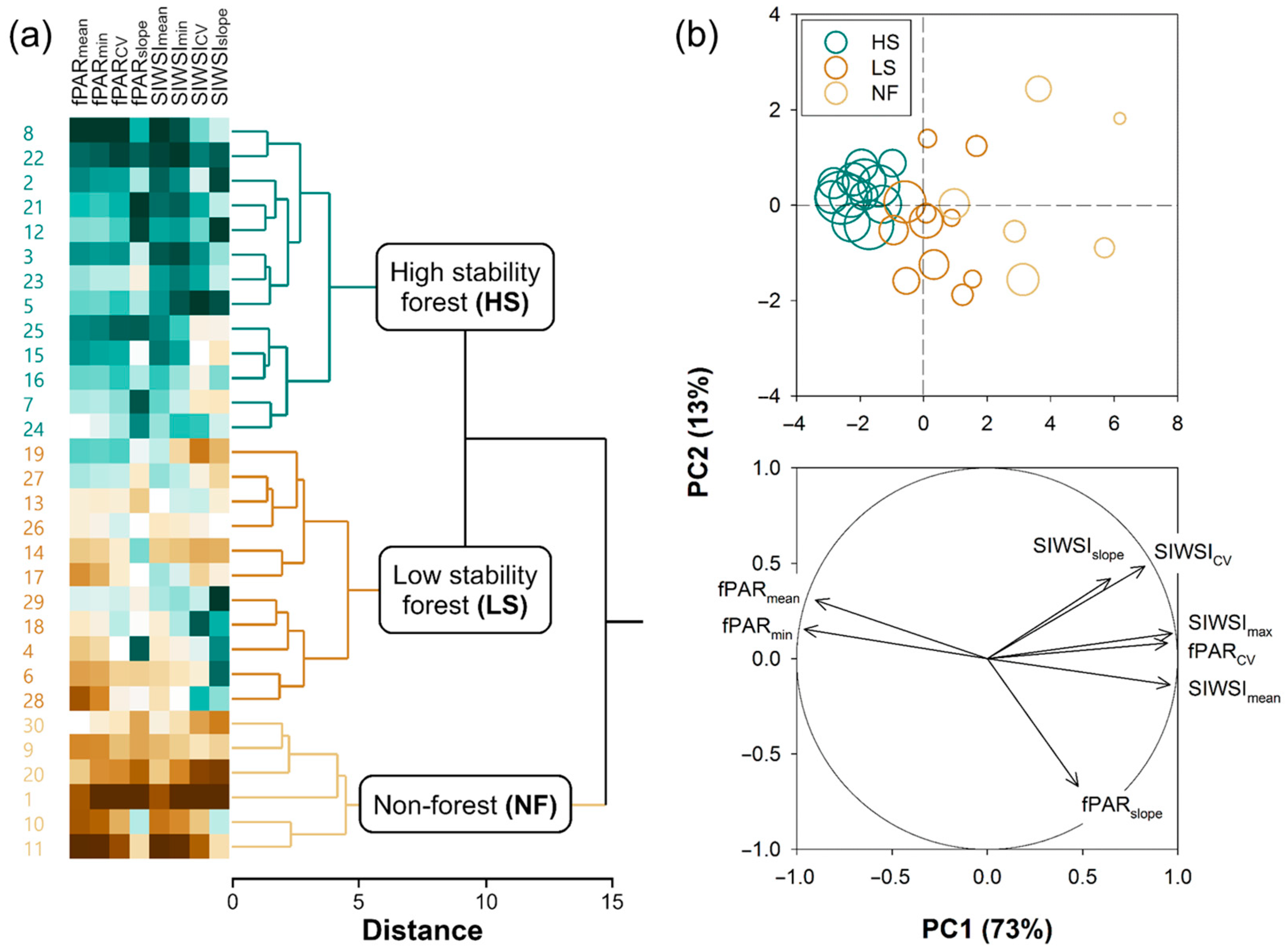
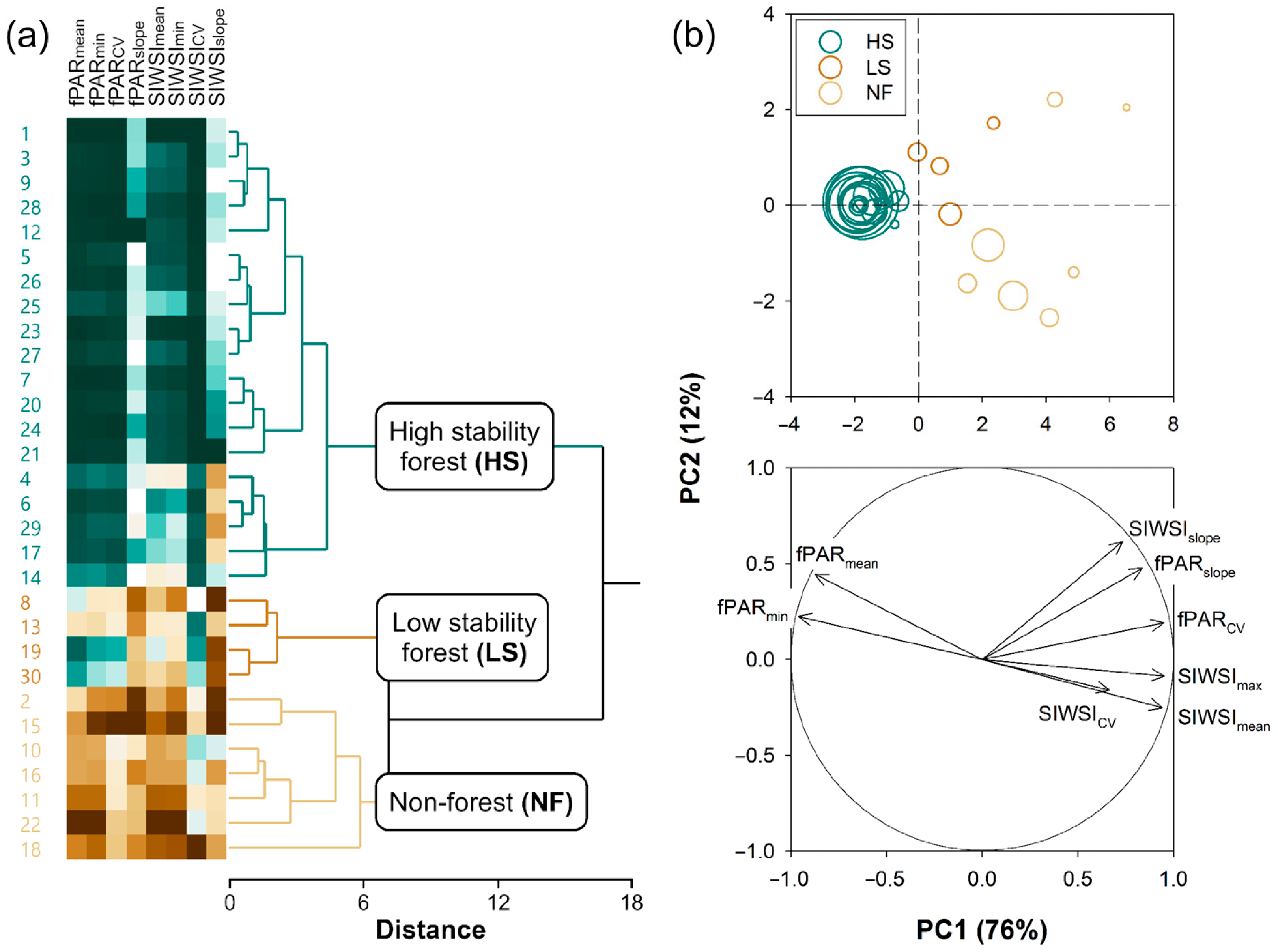
• HS forests to be characterized by high fPAR and low SIWSI mean values over the time series and fPAR minimum and SIWSI maximum values close to the means, with high temporal stability of these metrics, i.e., low CV and slope;
• LS forests to be characterized by lower fPAR and higher SIWSI mean values, more variable fPAR minimum and SIWSI maximum values, and less temporal stability, i.e., relatively high inter-annual fluctuation, high slope, or both; and
• NF areas to display the lowest fPAR and highest SIWSI mean values, and also highly variable fPAR minimum and SIWSI maximum values, together with a large temporal instability, i.e., high CV and/or slope.

Spatial analyses, including image processing, parameter calculation, and k-means clustering, were performed by using Google Earth Engine (GEE) Javascript API [60]. Hierarchical (Ward) clustering was performed by using the ‘stats’ package in R software [61]. A workflow of the methodological approach to mapping forest stability is provided in Supplementary Figure S1a.

2.3. Validation Framework

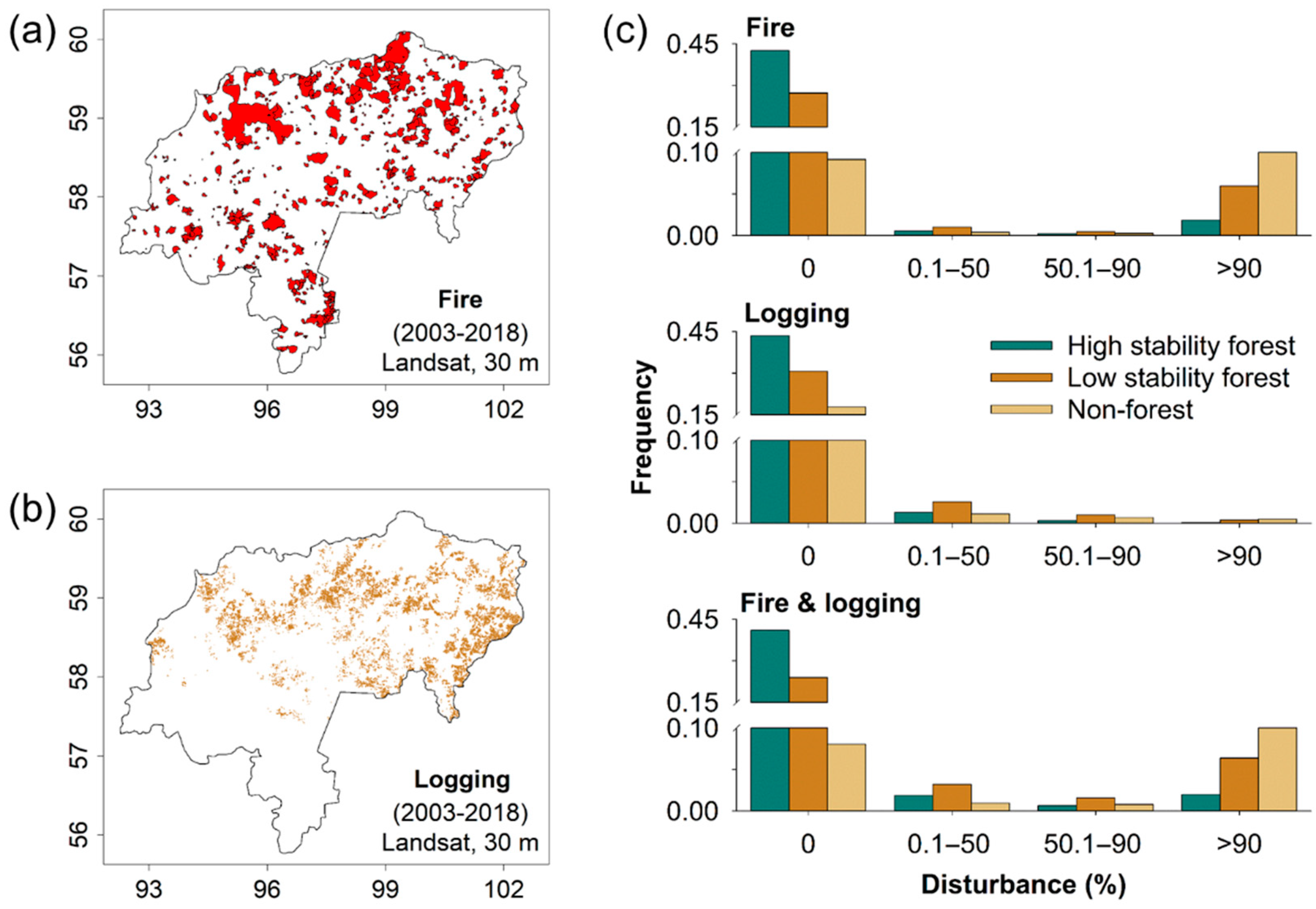
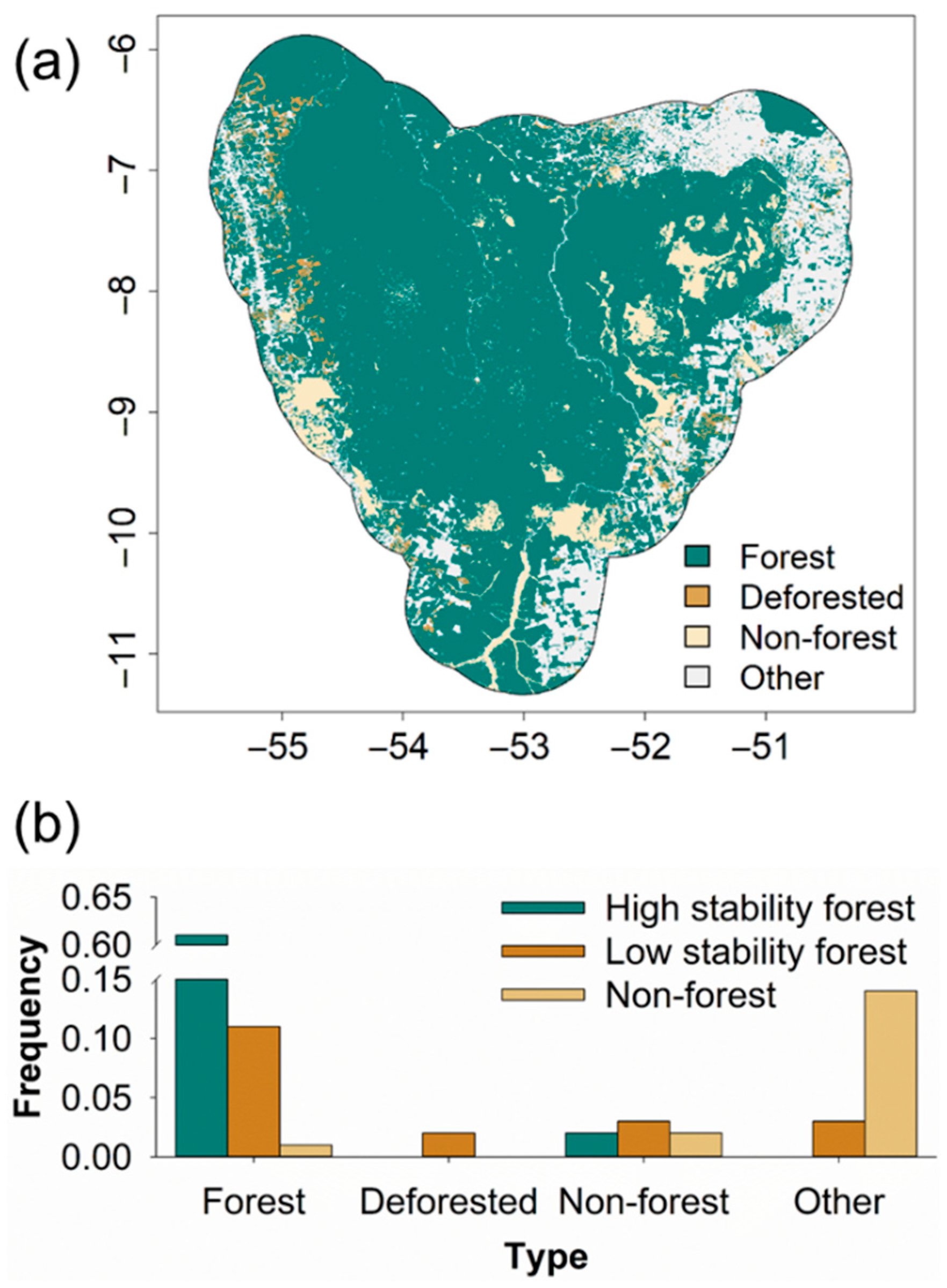
We validated our forest ecosystem stability spatial data layer for each study region with three independent sources of data and approaches. It is important to note, however, that currently available data products did not allow us to directly validate the low-stability (LS) class, precisely because our method is the first to categorize LS forests at landscape scales, using remote-sensing time series. First, the accuracy of our product was visually assessed against time series of remotely sensed reference imagery at randomly sampled locations within the study regions [62]. The reference dataset consisted of Landsat TM/ETM+/OLI imagery, which was used by an independent expert to establish whether a forest area within a MODIS pixel footprint had been disturbed during the past several decades [63]. This analysis covered the period from 1984 to 2018 and enabled tracking forest disturbances before (1984–2002) and during the study period (2003–2018). Poor pixels with low image quality or high cloud and shadow contaminations, which resulted in an insufficient level of certainty given by the expert (<50%), were removed from the analysis. The validation analysis focused on detecting changes in forest structure (i.e., tree canopy cover) to differentiate stable forests from forests with altered conditions. Areas of stable or disturbed forests were validated by using a probability-based stratified random sampling per biome. Our forest stability maps were used to create two major sub-strata per biome: no change, which corresponded to high stability forests (HS); and change, which was defined as highly disturbed, deforested, or non-forest (NF) areas. Low-stability (LS) forests were excluded from this analysis since this class represents more subtle changes in remotely sensed metrics of fPAR and SIWSI and often do not correspond to features that are visually detectable by using optical imagery (hence emphasizing the benefit of our approach). In total, 545 and 320 pixels were evaluated for the Southern Siberian taiga and the Kayapó territory. Image interpretation of time-series imagery was performed by using the Google Earth Timelapse app (https://earthengine.google.com/timelapse/; accessed on 19 November 2021).

Next, we compared stability classes with stand-disturbance history retrieved from a number of independent datasets over the period 2003–2018, as described below. For the southern taiga, we manually digitized areas with substantial forest-cover change corresponding to two major disturbances (fire and logging) over the period 2003–2018, using high-resolution Landsat imagery (ca. 30 m spatial resolution). The geographic area for validation comprised the Angara region, a deforestation hot spot in Siberia resulting from timber harvest and recurrent fires [50] that covers 12.7 million ha (i.e., ~10% of the study region). We used 30 m resolution data in order to retrieve information at a MODIS sub-pixel level, with the purpose of characterizing the relatively small areas of cut blocks and the heterogeneity of fire impacts. Fractions of MODIS pixels affected by either timber harvest or fire were generated separately. Thresholds of 10% and 90% were applied to these pixel fractions in order to identify areas with varying disturbance intensities: (i) undisturbed areas (<10% of each pixel affected by fire or logging), (ii) moderately disturbed areas (between 10% and 90%), and (iii) highly disturbed areas (>90%).

For the Kayapó territory, we used a recently updated deforestation spatial layer from the Brazilian space agency (PRODES and INPE), which is based on analysis of the Landsat archive (30 m spatial resolution) and provides information on the distribution of primary forests, degraded forests (mainly due to logging) and non-forest areas [64]. Using these data, we estimated the proportion of each of these categories within each MODIS pixel.

Finally, we evaluated the extent to which the mapped forest stability classes in both regions were consistent with estimates of tree canopy cover change, as reported in Reference [65]. This dataset provides information on areas experiencing tree cover loss or gain globally at ca. 30 m resolution. We evaluated the proportion of cumulative forest change over the period 2003–2018 within each MODIS pixel across the study regions. We applied the following threshold values: no change in tree cover (<10% of each pixel showing tree cover change), moderate change (between 10% and 90%), and substantially altered tree-cover areas (>90%). A summary of the datasets used for validation of the final forest stability maps is provided in Supplementary Figure S1b.

3. Results

The hierarchical clustering approach identified three classes based on MODIS time series of fPAR and SIWSI metrics for the southern taiga in Siberia (Figure 2a) and the Amazon rainforest in the Kayapó territory (Figure 3a). These classes captured 65% and 71% of the total variability present in the 30 k-means groups for Siberia and Kayapó, respectively. A PCA performed on the 30 k-means groups returned two principal components (PCs), which accounted for 86% and 88% of the total variance for the Southern Siberian taiga (Figure 2b) and the Kayapó territory (Figure 3b), respectively. These analyses unequivocally led to the definition of distinct classes of forest stability in both regions that are well illustrated by the loadings of each classificatory variable in the biplots shown in Figure 2b and Figure 3b. Particularly, high-stability (HS) forests were characterized by conditions representative of productive and stable forest ecosystems: high fPAR (mean and min), low SIWSI (mean and max), low CVs, and low absolute slopes (Figure 2 and Figure 3;

Table 1. Mean (±SD) values of variables derived from the fraction of photosynthetically active radiation intercepted by sunlit vegetation canopy (fPAR) and the shortwave infrared water stress index (SIWSI) across different forest stability classes for southern taiga ecoregion (Siberia, Russia) and Kayapó territory (Amazon basin, Brazil). The values were obtained from mean June–August fPAR and SIWSI values over the period 2003–2018. Slope (abs) denotes absolute slope values indicative of the presence or absence of temporal trends for both metrics. HS = high-stability forests; LS = low-stability forests; NF = non-forest areas.

	fPAR *				SIWSI
	Mean	Min	CV	Slope (abs)	Mean	Max	CV	Slope (abs)
Southern taiga ecoregion (Russia)
HS	86.77 ± 2.40	81.41 ± 3.12	0.03 ± 0.01	0.11 ± 0.09	−0.35 ± 0.03	−0.28 ± 0.05	0.05 ± 0.02	0.002 ± 0.002
LS	79.42 ± 6.01	72.67 ± 6.33	0.04 ± 0.01	0.24 ± 0.16	−0.29 ± 0.05	−0.18 ± 0.06	0.07 ± 0.02	0.003 ± 0.003
NF	72.65 ± 8.78	60.53 ± 10.73	0.08 ± 0.03	0.61 ± 0.42	−0.21 ± 0.07	−0.05 ± 0.10	0.10 ± 0.03	0.008 ± 0.006
Kayapó territory (Brazil)
HS	89.83 ± 0.26	89.03 ± 0.75	0.004 ± 0.002	0.56 ± 0.51	−0.35 ± 0.02	−0.33 ± 0.02	−0.03 ± 0.01	0.014 ± 0.012
LS	87.82 ± 2.01	84.30 ± 5.27	0.02 ± 0.02	3.48 ± 6.53	−0.26 ± 0.07	−0.17 ± 0.10	−0.22 ± 0.23	0.077 ± 0.084
NF	65.15 ± 8.14	56.62 ± 8.72	0.08 ± 0.03	17.36 ± 20.43	−0.09 ± 0.09	−0.01 ± 0.10	−0.64 ± 1.35	0.178 ± 0.206

* Scale factor of 100 applied to fPAR values.

). In contrast, low-stability (LS) forests were characterized by conditions of lower productivity and stability, including lower fPAR (mean and min), higher SIWSI (mean and max), higher CVs, and higher slope magnitudes (moderately higher in Siberia and much higher in Brazil; Figure 2 and Figure 3; Table 1). Finally, non-forested (NF) areas displayed the lowest fPAR (mean and min), the highest SIWSI (mean and max), and were much less stable than HS (higher CVs and slope magnitudes; Figure 2 and Figure 3; Table 1). Examples of representative time series of mean fPAR and SIWSI over the period 2003–2018 within each stability class and region are shown in Supplementary Figure S2.

The resulting regional forest stability layers revealed distinct spatial patterns that were consistent with other geospatial products, including higher-resolution imagery, digitized disturbance data, regional and global land-cover maps, and layers of tree-cover changes (see Section 2.3 for details). In particular, a visual comparison of forest stability maps with higher-resolution satellite images revealed a high level of agreement between stable forest canopies and areas clearly affected by human impacts (Figure 4c,d). The results of the visual expert assessment of structural changes in tree canopy cover over the period 1984–2018 showed a high accuracy of characterization of forest stability classes in both biomes (

Table 2. Estimated error matrix for expert validation of the resultant forest stability maps for southern taiga ecoregion (Siberia, Russia) and Kayapó territory (Amazon basin, Brazil). The validation is based on expert knowledge of the forested landscapes through the visual interpretation of changes in forest cover by using high-resolution imagery over the period 1984–2018. Forest stability classes are in rows, while the reference classes are in columns. This visual assessment was performed by using the Google Earth Timelapse app. All pixels for which expert certainty was low (<50%) were removed from the analysis. HS = high-stability forests; LS = low-stability forests; NF = non-forest areas.

Classified Data	Reference Data			User’s Accuracy (%)	Producer’s Accuracy (%)	Overall Accuracy (%)
	HS	NF	Total
Southern taiga ecoregion (Russia)
HS	381	3	384	99	91	92
NF	38	123	161	76	98
Total	419	126	545
Kayapó territory (Brazil)
HS	251	2	253	99	100	99
NF	1	66	67	99	97
Total	252	68	320

). In the southern taiga, the lowest user’s accuracy of 76%, reflecting commission error, was found in NF areas, and the lowest producer’s accuracy of 91%, reflecting omission error, was found for HS forests. In the Kayapó territory, both user’s and producer’s accuracies were above 97%. The overall accuracy was 92% for the boreal and 99% for the tropical biomes (Table 2). It is worth noting that our approach was able to capture the long-term effect of past disturbances occurring up to two decades before the study period (i.e., 1984–2002 period).

Importantly, a pixel-by-pixel comparison of our stability map to ten alternative runs of our approach by using different seeds for the random pixels used to train the k-means algorithm yielded consistent outputs (Supplementary Figure S3). Particularly, the lowest probability of a pixel to be assigned to a particular stability class was above 60% in both regions. Overall, the degree of agreement between our stability map and the alternative maps was 93% and 98% in the southern taiga and the Kayapó territory, respectively. Among the three stability classes, the highest degree of agreement was found for the high-stability forests (HS; 96% in the southern taiga and 99% in the Kayapó territory), followed by non-forest (NF) area (89% in the southern taiga and 100% in the Kayapó territory) and low-stability (LS) forest (90% in both regions).

Validation data on known fire and logging disturbances further confirmed the accuracy of the approach for the Angara region in Siberia (Figure 5). The majority of pixels classified as HS corresponded to a total lack of disturbance by either fire (79%) or logging (92%) during the study period. Pixels with intermediate levels of disturbance (up to 90%) corresponded mainly to LS (50%), and pixels showing high disturbance (>90%) were mainly represented by NF (56%). In the Kayapó territory, the vast majority of area mapped as primary forests according to the PRODES deforestation data was classified as HS (Figure 6), whereas areas mapped as deforested, non-forest, and other were dominated by LS and NF stability classes.

For additional validation, we compared our forest stability classes to a widely used dataset of global changes in tree canopy cover [65]. Consistent with our other comparisons, a majority of areas mapped as low forest loss or gain were classified as HS (58% and 72% for the southern taiga and Kayapó territory, respectively), whereas areas mapped as substantial forest loss or gain (change detected for >50% of a single MODIS pixel) were classified primarily as LS (30% and 60%) or NF (54% and 40%) (Supplementary Figure S4).

Overall, the HS class corresponded to forest patches having a relatively high tree canopy cover with minimal disturbance, which was the most prevalent category in Southern Siberia (54% of total land; Figure 4a) and in the Kayapó territory (63% of total land; Figure 4b). LS encompassed both degraded forests impacted by fires and human activity (e.g., logging, mining, or agricultural practices) over the study period (Figure 5 and Figure 6 and Supplementary Figure S3), as well as areas with naturally sparse vegetation cover. The latter was the case for the rear (i.e., southernmost) edge of the Southern Siberian taiga, which was characterized by a relatively low tree-cover density in the ecotone between the southernmost taiga and the forest steppe (Supplementary Figure S5a,c). LS accounted for 30% of the area in Southern Siberia and 19% in Kayapó. NF targeted areas with very low tree-cover density (Figure 1). These included natural treeless patches (e.g., grasslands or rocky areas) or, alternatively, deforested zones resulting from land conversion to agricultural fields, clear-cut or severe fires (Figure 5 and Figure 6 and Supplementary Figures S3 and S4), resulting in significant temporal (e.g., fires or logging) or permanent losses of tree cover (e.g., infrastructure development or agriculture). NF pixels accounted for 16% of the total area in Southern Siberia (Figure 4a) and 18% in Kayapó (Figure 4b).

4. Discussion

Here we defined forest stability classes derived from remote-sensing time-series data related to photosynthetic activity (fPAR) and water stress (SIWSI). These metrics are closely associated with ecophysiological processes that are indicative of photosynthetic activity and vegetation structure at the forest-stand and landscape levels [55,59], and the source data are readily available globally. The selection and interpretation of the metrics are informed by ecological theories of resource optimization, microclimate buffering, biological redundancy, and adaptive capacity [66,67]. We focused on representative regions of boreal and tropical forest because the majority of remaining primary forests are located in these biomes [68,69].

A large-scale validation dataset against which to measure the accuracy of our stability maps is not yet available, and particularly based on long-term ground truth data. Thus, to evaluate the accuracy of our approach, a few comparisons were made with other existing regional or global datasets which employed high-resolution data sources. Although these cannot fully substitute for validation data, they help to characterize the maps by yielding a degree of agreement between products that were derived entirely independently from one another. The results of the validation analyses suggest that our approach is applicable and sufficiently accurate to map forest stability (in terms of constancy) within boreal and tropical forest ecoregions. Both spatial and temporal assessments of forest stability classes showed consistent performance of our approach. The distinction between high-stability forests and non-forest areas showed a high level of agreement with other sources. On the other hand, the low stability class is, by its nature, difficult if not impossible to independently verify using existing products and optical imagery. This forest class is not necessarily subject to large-scale or intense disturbance but is, instead, more variant in time and susceptible to changing environmental conditions. Such dynamics can only be detected using long-term time series, a benefit of our approach compared to existing methods focused on distinct periods in time. It should also be noted that our digitized fire polygons in Siberia may represent either stand-replacing or non-stand-replacing fires, and that future work could further explore the impact of different fire severity levels on forest stability.

Our approach complements other approaches to assessing forest conditions globally. These include mapping intact forest landscapes [41], human pressure indicators [70,71,72,73], habitat fragmentation [74], tropical hinterland forests [22,75], and vegetation structural condition [76,77]. Each of these mapping techniques has its own advantages and limitations. For example, existing intact forest landscape layers provide information on globally consistent forested landscapes with little to no human interference [41], but they are intended to identify large forest masses (i.e., the associated patch size thresholds exclude valuable primary forests smaller than 50,000 ha), and the identified patches include non-forest land cover. Global evaluations of forest loss using standardized definitions can be used at a pixel level and can be useful for a wide variety of applications [65]. However, such definitions, based on tree canopy cover without complementary analysis of forest ecological conditions, equate heavily managed forests and tree plantations with primary forests, leading to potential misinterpretations and misuse [78].

Our approach to mapping forest stability bypasses some of these limitations by not relying on proxies of human influence, not requiring intensive machine-learning parameterization and training, and integrating multi-year information on time-series dynamics. It is also applicable across forest biomes and allows for the mapping of both large tracts and small patches of stable forests at any scale down to a minimum area consistent with that found necessary to maintain forest interior micro-environmental conditions (generally 500–2000 m) [79,80]. Smaller areas of stable forest constitute a substantial proportion of the natural forest cover in many regions [81], which are of considerable conservation value, including refugia habitat, biodiversity, and source populations for landscape restoration, among other ecosystem services [82,83,84,85,86].

While MODIS satellite imagery has coarser spatial resolution as compared with widely used Landsat data, we argue that this scale is appropriate for a landscape-level analysis of forest stability. By mapping the constancy property at a 500 m pixel resolution (~25 ha), we capture gradients in stability caused by edge effects, which have been estimated at over 1000 m for wet tropical forests (suggesting an absolute minimum area for a patch of undisturbed forest to be around 100 ha) [13,55] and 100–400 m for boreal and temperate forests (and a minimum patch of undisturbed forest being 1–16 ha) [87,88,89]. Boreal forest landscapes are naturally characterized by patches of different forest ecosystem types, including multiple seral stages following wildfire [90] which have been found to range in size from 2 to 650 ha. The spatial resolution of our analysis, therefore, is commensurate with the scaling of forests with a high level of stability in tropical biomes and for larger sized patches in boreal biomes. Likewise, by leveraging multi-year time series, we were able to capture the temporal dimension of forest degradation, which can take several years to manifest [91].

Our approach is limited in a number of important aspects that require further attention. The stability metric used was designed to address only the constancy property of stability, defined here as no major changes in forest canopy condition over a 16-year period (2003–2018). To evaluate the other two stability properties of resilience and persistence [30], consideration needs to be given to analyzing multi-patch dynamics and landscape-level metrics over a longer time series. For example, the available data are unable to represent resilience following state-altering disturbances and the potential for ecosystems to return to their pre-disturbed state or the optimum operating point given prevailing conditions (see Reference [92], for example). This is particularly relevant to boreal forests, where recurrent wildfires are part of their natural disturbance regime, and resilience needs to be considered from a landscape-wide perspective to take into account the shifting mosaic of seral stages over time. This is in contrast to tropical forests, which are characterized by a continuous closed canopy (i.e., projected foliage cover >70%) [93]. Thus, an expanse of structurally intact boreal forest canopy is unequivocally a stable forest, but patches of disturbed seral stages may be the result of either natural disturbances, especially wildfire, or human land-use impacts. On the other hand, loss of a structurally intact canopy in the wet tropics is a more reliable indicator of human rather than natural disturbance (notwithstanding impacts from large blowdowns [94] and tropical storms [95]).

Our stability metric did not distinguish between natural and anthropogenic disturbances. These contrasting dynamics could potentially be characterized by broken-line (segmented) regression methods [96], especially if progressively long time series of remotely sensed data are available. Uptrends and downtrends can also be used to help differentiate between vegetation greening and browning. In the tropics, longer series may particularly aid in disturbance detection since wet forests can reach a closed tree canopy within a few decades after disturbance. In the boreal, however, a second stage of analysis using finer spatial resolution satellite data and object-based image classification techniques [97] could potentially tease out human land-use impacts based upon their characteristic spatial patterning compared to those arising from natural disturbances [98]. Therefore, our approach is a first step towards mapping all three stability properties at a landscape scale [99].

Within a given ecoregion, our method also tends to classify naturally low-canopy-cover ecosystems as low stability compared with neighboring, relatively closed-canopy forests. The high-stability class is oriented, therefore, towards the more closed-canopy forests at an ecoregion level. Although the total area of lower-canopy ecosystems is minor in the southern taiga, possible variants of this methodology could employ metrics of habitat quality tailored to specific ecological units (e.g., land cover types), decouple fPAR magnitudes from stability metrics, or be mapped at a higher spatial resolution relevant to local-scale assessments, including through fusing of MODIS data with higher-spatial-resolution imagery, such as Landsat and Sentinel-2 (see Reference [100], for example). Finally, we note that this work has focused on two case-study forests that are typical of boreal and wet tropical forest ecosystems. Thus, further testing of the approach is needed in temperate and seasonally dry tropical forests.

Information on stable forests—including the constancy metric applied here—is relevant to national and international policies concerning biodiversity conservation and climate-change mitigation. At a national level, information about high-stability forests can be used to inform systematic conservation planning [101]. Information on the location of less stable forests is also relevant for ecological restoration, reforestation, and proforestation activities [102,103,104,105,106], or forestry intensification to alleviate logging pressure on primary forests [7,8,105]. Moreover, from a spatial ecology perspective, patches of disturbed forests are an inherent component of most temperate and boreal forest landscapes (see Reference [107], for example) and are valuable for biodiversity and the persistence of particular species dependent on early successional communities. In general, as long as enough of the surrounding forests are stable (i.e., resilient to disturbances—be they natural or anthropogenic), such ecosystems are sustainable [108].

5. Conclusions

Our methodology represents an ecophysiologically based approach to monitor and map ecosystem stability, as showcased for two contrasting forest biomes with the potential to be applied elsewhere. If upscaled and implemented globally, it would provide a uniform, objective source of information on a key property of forest ecosystems that is consistent with widely accepted definitions of primary forests. Recognizing the limitations of the approach, the data generated could be used as an independent source to cross-validate other local or global forest assessments. Because it is designed to be repeatable based on objective statistics with minimal expert intervention, assessments of global forest stability could be regularly updated by extending the time series as new satellite data become available. The information could be used to inform national and international policy settings that aim to prioritize conservation investments targeting stable forest ecosystems to maximize outcomes for biodiversity conservation, carbon storage, and other ecosystem services. Ecoregions that are still relatively free from the damaging impacts of large-scale human activities are rapidly disappearing, yet they provide valuable ecosystem service benefits to people. Because effective restoration can be costly and requires long-term management, identifying actions that can retain stable forests, including primary forests and intact forest landscapes, is a recommended strategy for advancing international commitments for conservation, biodiversity, and climate mitigation. Our approach, which maps the ecosystem stability of forests in terms of their constancy, contributes to the growing information based on the condition of forest ecosystems that remains an underassessed component of current global data layers.

References

1. FAO (Food and Agriculture Organization). The State of the World’s Forests 2020: Forests, Biodiversity and People; FAO: Rome, Italy, 2020. [Google Scholar] [CrossRef]
2. IUCN (International Union for Conservation of Nature). IUCN Policy Statement on Primary Forests Including Intact Forest Landscapes. In International Union for Conservation of Nature; IUCN: Glan, Switzerland, 2020; Available online: http://forestsandclimate.org.au/cms/wp-content/uploads/iucn-pf-ifl-policy-2020-approved-version-2-1.pdf (accessed on 13 July 2022).
3. FAO (Food and Agriculture Organization). Global Forest Resources Assessment 2020: Terms and Definitions. In Forest Resources Assessment Working Paper 188; FAO: Rome, Italy, 2020; Available online: http://www.fao.org/3/I8661EN/i8661en.pdf (accessed on 13 July 2022).
4. Thompson, I.D.; Guariguata, M.R.; Okabe, K.; Bahamondez, C.; Nasi, R.; Heymell, V.; Sabogal, C. An operational framework for defining and monitoring forest degradation. Ecol. Soc. 2013, 18, 20. [Google Scholar] [CrossRef]
5. Mackey, B.; DellaSala, D.A.; Kormos, C.; Lindenmayer, D.; Kumpel, N.; Zimmerman, B.; Hugh, S.; Young, V.; Foley, S.; Arsenis, K.; et al. Policy options for the world’s primary forests in multilateral environmental agreements. Conserv. Lett. 2015, 8, 139–147. [Google Scholar] [CrossRef] [Green Version]
6. Roche, P.K.; Campagne, C.S. From ecosystem integrity to ecosystem condition: A continuity of concepts supporting different aspects of ecosystem sustainability. Curr. Opin. Environ. Sustain. 2017, 29, 63–68. [Google Scholar] [CrossRef]
7. Kormos, C.F.; Mackey, B.; Della Sala, D.A.; Kumpe, N.; Jaeger, T.; Mittermeier, R.A.; Filardi, C. Primary forests: Definition, status and future prospects for global conservation. In Encyclopedia of the Anthropocene; DellaSala, D.A., Goldstein, M.I., Eds.; Elsevier: Oxford, UK, 2018; Volume 2, pp. 31–41. [Google Scholar] [CrossRef]
8. Watson, J.E.M.; Evans, T.; Venter, O.; Williams, B.; Tulloch, A.; Stewart, C.; Thompson, I.; Ray, J.C.; Murray, K.; Salazar, A.; et al. The exceptional value of intact forest ecosystems. Nat. Ecol. Evol. 2018, 2, 599–610. [Google Scholar] [CrossRef]
9. Funk, J.M.; Aguilar-Amuchastegui, N.; Baldwin-Cantello, W.; Busch, J.; Chuvasov, E.; Evans, T.; Griffin, B.; Harris, N.; Ferreira, M.N.; Petersen, K.; et al. Securing the climate benefits of stable forests. Clim. Policy 2019, 19, 845–860. [Google Scholar] [CrossRef] [Green Version]
10. Thom, D.; Golivets, M.; Edling, L.; Meigs, G.W.; Gourevitch, J.D.; Sonter, L.J.; Galford, G.L.; Keeton, W.S. The climate sensitivity of carbon, timber, and species richness covaries with forest age in boreal–temperate North America. Glob. Chang. Biol. 2019, 25, 2446–2458. [Google Scholar] [CrossRef]
11. Mackey, B.; Kormos, C.F.; Keith, H.; Moomaw, W.R.; Houghton, R.A.; Mittermeier, R.A.; Hole, D.; Hugh, S. Understanding the importance of primary tropical forest protection as a mitigation strategy. Mitig. Adapt. Strateg. Glob. Chang. 2020, 25, 763–787. [Google Scholar] [CrossRef] [Green Version]
12. Asner, G.; Knapp, D.E.; Broadbent, E.N.; Oliveira, J.C.; Keller, M.; Silva, J.N. Selective logging in the Brazilian Amazon. Science 2005, 310, 480–482. [Google Scholar] [CrossRef]
13. Broadbent, E.N.; Asner, G.P.; Keller, M.; Knapp, D.E.; Oliveira, P.J.C.; Silva, J.N. Forest fragmentation and edge effects from deforestation and selective logging in the Brazilian Amazon. Biol. Conserv. 2008, 141, 1745–1757. [Google Scholar] [CrossRef]
14. Tyukavina, A.; Hansen, M.C.; Potapov, P.V.; Stehman, S.V.; Smith-Rodriguez, K.; Okpa, C.; Aguilar, R. Types and rates of forest disturbance in Brazilian Legal Amazon, 2000–2013. Sci. Adv. 2017, 3, e1601047. [Google Scholar] [CrossRef] [Green Version]
15. Herold, M.; Román-Cuesta, R.M.; Mollicone, D.; Hirata, Y.; van Laake, P.; Asner, G.P.; Souza, C.; Skutsch, M.; Avitabile, V.; MacDicken, K. Options for monitoring and estimating historical carbon emissions from forest degradation in the context of REDD+. Carbon Balance Manag. 2011, 6, 13. [Google Scholar] [CrossRef] [Green Version]
16. Gao, Y.; Skutsch, M.; Paneque-Gálvez, J.; Ghilardi, A. Remote sensing of forest degradation: A review. Environ. Res. Lett. 2020, 15, 103001. [Google Scholar] [CrossRef]
17. Lambin, E.F. Monitoring forest degradation in tropical regions by remote sensing: Some methodological issues. Glob. Ecol. Biogeogr. 1999, 8, 191–198. [Google Scholar] [CrossRef]
18. Berenguer, E.; Ferreira, J.; Gardner, T.A.; Aragao, L.E.O.C.; de Camargo, P.B.; Cerri, C.E.; Durigan, M.; Cosme De Oliveira, R.J.; Guimarães Vieira, I.C.; Barlow, J. A large-scale field assessment of carbon stocks in human-modified tropical forests. Glob. Chang. Biol. 2014, 20, 3713–3726. [Google Scholar] [CrossRef] [Green Version]
19. Baccini, A.; Walker, W.; Carvalho, L.; Farina, M.; Sulla-Menashe, D.; Houghton, R.A. Tropical forests are a net carbon source based on aboveground measurements of gain and loss. Science 2017, 358, 230–233. [Google Scholar] [CrossRef] [Green Version]
20. Mitchell, A.L.; Rosenqvist, A.; Mora, B. Current remote sensing approaches to monitoring forest degradation in support of countries measurement, reporting and verification (MRV) systems for REDD+. Carbon Balance Manag. 2017, 12, 9. [Google Scholar] [CrossRef] [Green Version]
21. Potapov, P.; Li, X.; Hernandez-Serna, A.; Tyukavina, A.; Hansen, M.C.; Kommareddy, A.; Pickens, A.; Turubanova, S.; Tang, H.; Silva, C.E.; et al. Mapping and monitoring global forest canopy height through integration of GEDI and Landsat data. Remote Sens. Environ. 2020, 253, 112165. [Google Scholar] [CrossRef]
22. Turubanova, S.; Potapov, P.V.; Tyukavina, A.; Hansen, M.C. Ongoing primary forest loss in Brazil, Democratic Republic of the Congo, and Indonesia. Environ. Res. Lett. 2018, 13, 074028. [Google Scholar] [CrossRef] [Green Version]
23. Bergeron, Y.; Fenton, N.J. Boreal forests of eastern Canada revisited: Old growth, nonfire disturbances, forest succession, and biodiversity. Botany 2012, 90, 509–523. [Google Scholar] [CrossRef]
24. Martin, M.; Morin, H.; Fenton, N.J. Secondary disturbances of low and moderate severity drive the dynamics of eastern Canadian boreal old-growth forests. Ann. For. Sci. 2019, 76, 108. [Google Scholar] [CrossRef]
25. Senf, C.; Pflugmacher, D.; Hostert, P.; Seidl, R. Using Landsat time series for characterizing forest disturbance dynamics in the coupled human and natural systems of Central Europe. ISPRS J. Photogramm. Remote Sens. 2017, 130, 453–463. [Google Scholar] [CrossRef] [PubMed]
26. Levin, S.A.; Grenfell, B.; Hastings, A.; Perelson, A.S. Mathematical and computational challenges in population biology and ecosystems science. Science 1997, 275, 334–343. [Google Scholar] [CrossRef] [Green Version]
27. Carnahan, J.A. Mapping Australia’s vegetation—200 years of change. Cartography 1990, 19, 1–6. [Google Scholar] [CrossRef]
28. Gauthier, S.; De Grandpré, L.; Bergeron, Y. Differences in forest composition in two boreal forest ecoregions of Quebec. J. Veg. Sci. 2000, 11, 781–790. [Google Scholar] [CrossRef]
29. Chávez, V.; Macdonald, S.E. The influence of canopy patch mosaics on understory plant community composition in boreal mixedwood forest. For. Ecol. Manag. 2010, 259, 1067–1075. [Google Scholar] [CrossRef]
30. Grimm, V.; Wissel, C. Babel, or the ecological stability discussions: An inventory and analysis of terminology and a guide for avoiding confusion. Oecologia 1997, 109, 323–334. [Google Scholar] [CrossRef]
31. Hughes, J.B.; Ives, A.R.; Norberg, J. Do species interactions buffer environmental variation (in theory)? In Biodiversity and Ecosystem Functioning. Synthesis and Perspectives; Loreau, M., Naeem, S., Inchausti, P., Eds.; Oxford University Press: Oxford, UK, 2002; pp. 92–101. [Google Scholar]
32. Loreau, M.; Downing, A.; Emmerson, M.; Gonzalez, A.; Hughes, J.; Inchausti, P.; Joshi, J.; Norberg, J.; Sala, O. A new look at the relationship between diversity and stability. In Biodiversity and Ecosystem Functioning. Synthesis and Perspectives; Loreau, M., Naeem, S., Inchausti, P., Eds.; Oxford University Press: Oxford, UK, 2002; pp. 79–91. [Google Scholar]
33. Roderick, M.L.; Berry, S.L.; Noble, I.R. A framework for understanding the linkage between environment and vegetation based on the surface area to volume ratio of leaves. Funct. Ecol. 2000, 14, 423–437. [Google Scholar] [CrossRef]
34. Migliavacca, M.; Musavi, T.; Mahecha, M.D.; Nelson, J.A.; Knauer, J.; Baldocchi, D.D.; Perez-Priego, O.; Christiansen, R.; Peters, J.; Anderson, K.; et al. The three major axes of terrestrial ecosystem function. Nature 2021, 598, 468–472. [Google Scholar] [CrossRef]
35. Sellers, P.J. Canopy reflectance, photosynthesis and transpiration. Int. J. Remote Sens. 1985, 6, 1335–1372. [Google Scholar] [CrossRef]
36. Berry, S.; Mackey, B.; Brown, T. Potential applications of remotely sensed vegetation greenness to habitat analysis and the conservation of dispersive fauna. Pac. Conserv. Biol. 2007, 13, 120–127. [Google Scholar] [CrossRef]
37. Tucker, C.J.; Sellers, P.J. Satellite remote sensing of primary production. Int. J. Remote Sens. 1986, 7, 1395–1416. [Google Scholar] [CrossRef]
38. Prince, S.D. A model of regional primary production for use with course resolution satellite data. Int. J. Remote Sens. 1991, 12, 1313–1330. [Google Scholar] [CrossRef]
39. Sims, D.A.; Gamon, J.A. Estimation of vegetation water content and photosynthetic tissue area from spectral reflectance: A comparison of indices based on liquid water and chlorophyll absorption features. Remote Sens. Environ. 2003, 84, 526–537. [Google Scholar] [CrossRef]
40. Peñuelas, J.; Filella, I.; Biel, C.; Serrano, L.; Save, R. The reflectance at the 950–970 nm region as an indicator of plant water status. Int. J. Remote Sens. 1993, 14, 1887–1905. [Google Scholar] [CrossRef]
41. Potapov, P.; Hansen, M.C.; Laestadius, L.; Turubanova, S.; Yaroshenko, A.; Thies, C.; Smith, W.; Zhuravleva, I.; Komarova, A.; Minnemeyer, S.; et al. The last frontiers of wilderness: Tracking loss of intact forest landscapes from 2000 to 2013. Sci. Adv. 2017, 3, e1600821. [Google Scholar] [CrossRef] [Green Version]
42. Achard, F.; Mollicone, D.; Stibig, H.J.; Aksenov, D.; Laestadius, L.; Li, Z.; Potapov, P.; Yaroshenko, A. Areas of rapid forest-cover change in boreal Eurasia. For. Ecol. Manag. 2006, 237, 322–334. [Google Scholar] [CrossRef]
43. Cochrane, M.A.; Laurance, W.F. Synergisms among fire, land use, and climate change in the Amazon. AMBIO J. Hum. Environ. 2008, 37, 522–527. [Google Scholar] [CrossRef] [PubMed]
44. Cochrane, M.A.; Laurance, W.F. Fire as a large-scale edge effect in Amazonian forests. J. Trop. Ecol. 2002, 18, 311–325. [Google Scholar] [CrossRef] [Green Version]
45. Cochrane, M.A. Fire science for rainforests. Nature 2003, 421, 913–919. [Google Scholar] [CrossRef]
46. Achard, F.; Eva, H.D.; Mollicone, D.; Beuchle, R. The effect of climate anomalies and human ignition factor on wildfires in Russian boreal forests. Philos. Trans. R. Soc. B Biol. Sci. 2008, 363, 2331–2339. [Google Scholar] [CrossRef] [Green Version]
47. Kukavskaya, E.A.; Buryak, L.V.; Ivanova, G.; Conard, S.; Kalenskaya, O.; Zhila, S.V.; McRae, D.J. Influence of logging on the effects of wildfire in Siberia. Environ. Res. Lett. 2013, 8, 045034. [Google Scholar] [CrossRef]
48. Matricardi, E.A.T.; Skole, D.L.; Costa, O.B.; Pedlowski, M.A.; Samek, J.H.; Miguel, E.P. Long-term forest degradation surpasses deforestation in the Brazilian Amazon. Science 2020, 369, 1378–1382. [Google Scholar] [CrossRef] [PubMed]
49. Garrett, R.D.; Cammelli, F.; Ferreira, J.; Levy, S.A.; Valentim, J.; Vieira, I. Forests and Sustainable Development in the Brazilian Amazon: History, Trends, and Future Prospects. Annu. Rev. Environ. Resour. 2021, 46, 625–652. [Google Scholar] [CrossRef]
50. Shvetsov, E.G.; Kukavskaya, E.A.; Shestakova, T.A.; Laflamme, J.; Rogers, B.M. Increasing fire and logging disturbances in Siberian boreal forests: A case study of the Angara region. Environ. Res. Lett. 2021, 16, 115007. [Google Scholar] [CrossRef]
51. Alexeyev, V.A.; Birdsey, R.A. Carbon Storage in Forests and Peatlands of Russia; General Technical Report NE-244; USDA Forest Service: Radnor, PA, USA, 1998. [Google Scholar] [CrossRef]
52. Soja, A.J.; Cofer, W.R.; Shugart, H.H.; Sukhinin, A.I.; Stackhouse, P.W., Jr.; McRae, D.J.; Conard, S.G. Estimating fire emissions and disparities in boreal Siberia (1998–2002). J. Geophys. Res. 2004, 109, D14S06. [Google Scholar] [CrossRef]
53. Myneni, R.; Knyazikhin, Y.; Park, T. MCD15A3H MODIS/Terra + Aqua Leaf Area Index/FPAR 4-Day L4 Global 500 m SIN Grid V006 [Data Set]; NASA EOSDIS LP DAAC: Sioux Falls, SD, USA, 2015. [Google Scholar] [CrossRef]
54. Fensholt, R.; Sandholt, I. Derivation of a shortwave infrared water stress index from MODIS near- and shortwave infrared data in a semiarid environment. Remote Sens. Environ. 2003, 87, 111–121. [Google Scholar] [CrossRef]
55. Briant, G.; Gond, V.; Laurance, S.G.W. Habitat fragmentation and the desiccation of forest canopies: A case study from eastern Amazonia. Biol. Conserv. 2010, 143, 2763–2769. [Google Scholar] [CrossRef]
56. Friedl, M.; Sulla-Menashe, D. MCD12Q1 MODIS/Terra + Aqua Land Cover Type Yearly L3 Global 500 m SIN Grid V006 [Data Set]; NASA EOSDIS LP DAAC: Sioux Falls, SD, USA, 2019. [Google Scholar] [CrossRef]
57. Enderle, D.I.M.; Weih, R.C., Jr. Integrating supervised and unsupervised classification methods to develop a more accurate land cover classification. J. Ark. Acad. Sci. 2005, 59, 10. [Google Scholar]
58. Ward, J.H. Hierarchical grouping to optimize an objective function. J. Am. Stat. Assoc. 1963, 58, 236–244. [Google Scholar] [CrossRef]
59. Mackey, B.; Berry, S.; Hugh, S.; Ferrier, S.; Harwood, T.D.; Williams, K.J. Ecosystem greenspots: Identifying potential drought, fire, and climate-change micro-refuges. Ecol. Appl. 2012, 22, 1852–1864. [Google Scholar] [CrossRef] [Green Version]
60. Gorelick, N.; Hancher, M.; Dixon, M.; Ilyushchenko, S.; Thau, D.; Moore, R. Google Earth Engine: Planetary-scale geospatial analysis for everyone. Remote Sens. Environ. 2017, 202, 18–27. [Google Scholar] [CrossRef]
61. R Core Team. R: A Language and Environment for Statistical Computing; R Foundation for Statistical Computing: Vienna, Austria, 2022; Available online: https://www.r-project.org (accessed on 13 July 2022).
62. Stehman, S.V.; Czaplewski, R.L. Design and analysis for thematic map accuracy assessment: Fundamental principles. Remote Sens. Environ. 1998, 64, 331–344. [Google Scholar] [CrossRef]
63. Hislop, S.; Haywood, A.; Alaibakhsh, M.; Nguyen, T.H.; Soto-Berelov, M.; Jones, S.; Stone, C. A reference data framework for the application of satellite time series to monitor forest disturbance. Int. J. Appl. Earth Obs. Geoinf. 2021, 105, 102636. [Google Scholar] [CrossRef]
64. INPE (Instituto Nacional de Pesquisas Espaciais). Projeto PRODES: Monitoramento da Floresta Amazônica Brasileira por Satélite [Data Set]; INPE: São José dos Campos, Brasil, 2019; Available online: http://www.obt.inpe.br/prodes (accessed on 19 November 2021).
65. Hansen, M.C.; Potapov, P.V.; Moore, R.; Hancher, M.; Turubanova, S.A.; Tyukavina, A.; Thau, D.; Stehman, S.V.; Goetz, S.J.; Loveland, T.R.; et al. High-resolution global maps of 21st-century forest cover change. Science 2013, 342, 850–853. [Google Scholar] [CrossRef] [Green Version]
66. Packham, J.R.; Harding, D.J.L.; Hilton, G.M.; Stuttard, R.A. Functional Ecology of Woodlands and Forests; Chapman and Hall: London, UK, 1992. [Google Scholar]
67. Larsen, J.B. Ecological stability of forests and sustainable silviculture. For. Ecol. Manag. 1994, 73, 85–96. [Google Scholar] [CrossRef]
68. FAO (Food and Agriculture Organization). Global Forest Resources Assessment 2020: Main Report; FAO: Rome, Italy, 2020. [Google Scholar] [CrossRef]
69. Mackey, B.; Skinner, E.; Norman, P. A Review of Current Reporting and Available Data on Primary Forest and Potential Methods for Country-Level Assessment; FAO: Rome, Italy, 2020; Available online: http://assets.fsnforum.fao.org.s3-eu-west-1.amazonaws.com/public/files/163_Primary_Forests/DRAFT_Primary_Forest_Report_12Feb20.pdf (accessed on 13 July 2022).
70. Venter, O.; Sanderson, E.W.; Magrach, A.; Allan, J.R.; Beher, J.; Jones, K.R.; Possingham, H.P.; Laurance, W.F.; Wood, P.; Fekete, B.M.; et al. Global terrestrial Human Footprint maps for 1993 and 2009. Sci. Data 2016, 3, 160067. [Google Scholar] [CrossRef] [Green Version]
71. Ibisch, P.L.; Hoffmann, M.T.; Kreft, S.; Pe′Er, G.; Kati, V.; Biber-Freudenberger, L.; DellaSala, D.A.; Vale, M.M.; Hobson, P.R.; Selva, N. A global map of roadless areas and their conservation status. Science 2016, 354, 1423–1427. [Google Scholar] [CrossRef] [PubMed]
72. Beyer, H.L.; Venter, O.; Grantham, H.S.; Watson, J.E.M. Substantial losses in ecoregion intactness highlight urgency of globally coordinated action. Conserv. Lett. 2020, 13, e12692. [Google Scholar] [CrossRef]
73. Grantham, H.S.; Duncan, A.; Evans, T.D.; Jones, K.; Beyer, H.; Schuster, R.; Walston, J.; Ray, J.; Robinson, J.; Callow, M.; et al. Modification of forests by people means only 40% of remaining forests have high ecosystem integrity. bioRxiv 2020. [Google Scholar] [CrossRef]
74. Haddad, N.M.; Brudvig, L.A.; Clobert, J.; Davies, K.F.; Gonzalez, A.; Holt, R.D.; Lovejoy, T.E.; Sexton, J.O.; Austin, M.P.; Collins, C.D.; et al. Habitat fragmentation and its lasting impact on Earth’s ecosystems. Sci. Adv. 2015, 1, e1500052. [Google Scholar] [CrossRef] [Green Version]
75. Tyukavina, A.; Hansen, M.C.; Potapov, P.V.; Krylov, A.M.; Goetz, S.J. Pan-tropical hinterland forests: Mapping minimally disturbed forests. Glob. Ecol. Biogeogr. 2016, 25, 151–163. [Google Scholar] [CrossRef]
76. Hansen, A.; Barnett, K.; Jantz, P.; Phillips, L.; Goetz, S.J.; Hansen, M.C.; Venter, O.; Watson, J.E.M.; Burns, P.; Atkinson, S.; et al. Global humid tropics forest structural condition and forest structural integrity maps. Sci. Data 2019, 6, 232. [Google Scholar] [CrossRef] [PubMed] [Green Version]
77. Hansen, A.J.; Burns, P.; Ervin, J.; Goetz, S.J.; Hansen, M.; Venter, O.; Watson, J.E.M.; Jantz, P.A.; Virnig, A.L.S.; Barnett, K.; et al. A policy-driven framework for conserving the best of Earth’s remaining moist tropical forests. Nat. Ecol. Evol. 2020, 4, 1377–1384. [Google Scholar] [CrossRef] [PubMed]
78. Tropek, R.; Sedláček, O.; Beck, J.; Keil, P.; Musilová, Z.; Šímová, I.; Storch, D. Comment on “High-resolution global maps of 21st-century forest cover change”. Science 2014, 344, 981. [Google Scholar] [CrossRef] [Green Version]
79. Laurance, W.F.; Laurance, S.G.; Ferreira, L.V.; RankindeMerona, J.M.; Gascon, C.; Lovejoy, T.E. Biomass collapse in Amazonian forest fragments. Science 1997, 278, 1117–1118. [Google Scholar] [CrossRef]
80. Chaplin-Kramer, R.; Ramler, I.; Sharp, R.; Haddad, N.M.; Gerber, J.S.; West, P.C.; Mandle, L.; Engstrom, P.; Baccini, A.; Sim, S.; et al. Degradation in carbon stocks near tropical forest edges. Nat. Commun. 2015, 6, 10158. [Google Scholar] [CrossRef]
81. Chazdon, R.L.; Brancalion, P.H.S.; Laestadius, L.; Bennett-Curry, A.; Buckingham, K.; Kumar, C.; Moll-Rocek, J.; Vieira, I.C.G.; Wilson, S.J. When is a forest a forest? Forest concepts and definitions in the era of forest and landscape restoration. Ambio 2016, 45, 538–550. [Google Scholar] [CrossRef]
82. Hernández-Ruedas, M.A.; Arroyo-Rodríguez, V.; Meave, J.A.; Martínez-Ramos, M.; Ibarra-Manríquez, G.; Martínez, E.; Jamangapé, G.; Melo, F.P.L.; Santos, B.A. Conserving tropical tree diversity and forest structure: The value of small rainforest patches in moderately-managed landscapes. PLoS ONE 2014, 9, e98931. [Google Scholar] [CrossRef] [Green Version]
83. Le Roux, D.S.; Ikin, K.; Lindenmayer, D.B.; Manning, A.D.; Gibbons, P. Single large or several small? Applying biogeographic principles to tree-level conservation and biodiversity offsets. Biol. Conserv. 2015, 191, 558–566. [Google Scholar] [CrossRef]
84. Tulloch, A.I.T.; Barnes, M.D.; Ringma, J.; Fuller, R.A.; Watson, J.E.M. Understanding the importance of small patches of habitat for conservation. J. Appl. Ecol. 2016, 53, 418–429. [Google Scholar] [CrossRef] [Green Version]
85. Häkkilä, M.; Savilaakso, S.; Johansson, A.; Sandgren, T.; Uusitalo, A.; Mönkkönen, M.; Puttonen, P. Do small protected habitat patches within boreal production forests provide value for biodiversity conservation? A systematic review protocol. Environ. Evid. 2019, 8, 30. [Google Scholar] [CrossRef]
86. Wintle, B.A.; Kujala, H.; Whitehead, A.; Cameron, A.; Veloz, S.; Kukkala, A.; Moilanen, A.; Gordon, A.; Lentini, P.E.; Cadenhead, N.C.R.; et al. Global synthesis of conservation studies reveals the importance of small habitat patches for biodiversity. Proc. Natl. Acad. Sci. USA 2019, 116, 909–914. [Google Scholar] [CrossRef] [PubMed] [Green Version]
87. Boucher, Y.; St-Laurent, M.H.; Grondin, P. Logging-induced edge and configuration of old-growth forest remnants in the eastern North American boreal forests. Nat. Areas J. 2011, 31, 300–306. [Google Scholar] [CrossRef]
88. Dantas De Paula, M.; Groeneveld, J.; Huth, A. The extent of edge effects in fragmented landscapes: Insights from satellite measurements of tree cover. Ecol. Indic. 2016, 69, 196–204. [Google Scholar] [CrossRef]
89. De Frenne, P.; Lenoir, J.; Luoto, M.; Scheffers, B.R.; Zellweger, F.; Aalto, J.; Ashcroft, M.B.; Christiansen, D.M.; Decocq, G.; De Pauw, K.; et al. Forest microclimates and climate change: Importance, drivers and future research agenda. Glob. Chang. Biol. 2021, 27, 2279–2297. [Google Scholar] [CrossRef]
90. Sims, R.A.; Mackey, B.G.; Baldwin, K.A. Stand and landscape level applications of a forest ecosystem classification for Northwestern Ontario, Canada. Ann. For. Sci. 1995, 52, 573–588. [Google Scholar] [CrossRef] [Green Version]
91. Ibáñez, I.; Katz, D.S.; Peltier, D.; Wolf, S.M.; Connor Barrie, B.T. Assessing the integrated effects of landscape fragmentation on plants and plant communities: The challenge of multiprocess-multiresponse dynamics. J. Ecol. 2014, 102, 882–895. [Google Scholar] [CrossRef] [Green Version]
92. Kay, J.J.; Regier, H.A. Uncertainty, complexity, and ecological integrity: Insights from an ecosystem approach. In Implementing Ecological Integrity; Crabbé, P., Holland, A., Ryszkowski, L., Westra, L., Eds.; Springer: Dordrecht, the Netherlands, 2000; pp. 121–156. [Google Scholar] [CrossRef]
93. Specht, R.L. Vegetation. In The Australian Environment, 4th ed.; Leeper, G.W., Ed.; CSIRO and Melbourne University Press: Melbourne, Australia, 1970; pp. 44–67. [Google Scholar]
94. Nelson, B.W.; Kapos, V.; Adams, J.B.; Oliveira, W.J.; Braun, O.P.G. Forest disturbance by large blowdowns in the Brazilian Amazon. Ecology 1994, 75, 853–858. [Google Scholar] [CrossRef]
95. Ibanez, T.; Keppel, G.; Menkes, C.; Gillespie, T.W.; Lengaigne, M.; Mangeas, M.; Rivas-Torres, G.; Birnbaum, P. Globally consistent impact of tropical cyclones on the structure of tropical and subtropical forests. J. Ecol. 2019, 107, 279–292. [Google Scholar] [CrossRef]
96. Robbins, K.R.; Saxton, A.M.; Southern, L.L. Estimation of nutrient requirements using broken-line regression analysis. J. Anim. Sci. 2006, 84, E155–E165. [Google Scholar] [CrossRef]
97. Ma, L.; Li, M.; Ma, X.; Cheng, L.; Du, P.; Liu, Y. A review of supervised object-based land-cover image classification. ISPRS J. Photogramm. Remote Sens. 2017, 130, 277–293. [Google Scholar] [CrossRef]
98. Boucher, D.; De Grandpré, L.; Kneeshaw, D.; St-Onge, B.; Ruel, J.C.; Waldron, K.; Lussier, J.M. Effects of 80 years of forest management on landscape structure and pattern in the eastern Canadian boreal forest. Landsc. Ecol. 2015, 30, 1913–1929. [Google Scholar] [CrossRef]
99. Jentsch, A.; Beierkuhnlein, C.; White, P.S. Scale, the dynamic stability of forest ecosystems, and the persistence of biodiversity. Silva. Fenn. 2002, 36, 393–400. [Google Scholar] [CrossRef] [Green Version]
100. Wulder, M.A.; Hall, R.J.; Coops, N.C.; Franklin, S.E. High spatial resolution remotely sensed data for ecosystem characterization. Bioscience 2004, 54, 511–521. [Google Scholar] [CrossRef] [Green Version]
101. Mackey, B.; Watson, J.; Worboys, G.L. Connectivity Conservation and the Great Eastern Ranges Corridor: An Independent Report to the Interstate Agency Working Group (Alps to Atherton Connectivity Conservation Working Group) Convened under the Environment Heritage and Protection Council/Natural Resource Management Ministerial Council; Department of Environment, Climate Change and Water NSW: Sydney, Australia, 2010; Available online: https://conservationcorridor.org/cpb/Mackey_et_al_2010.pdf (accessed on 13 July 2022).
102. Griscom, B.W.; Adams, J.; Ellis, P.W.; Houghton, R.A.; Lomax, G.; Miteva, D.A.; Schlesinger, W.H.; Shoch, D.; Siikamäki, J.V.; Smith, P.; et al. Natural climate solutions. Proc. Natl. Acad. Sci. USA 2017, 114, 11645–11650. [Google Scholar] [CrossRef] [PubMed] [Green Version]
103. IPCC (Intergovernmental Panel on Climate Change). Summary for Policymakers. In Global Warming of 1.5 °C. An IPCC Special Report on the Impacts of Global Warming of 1.5 °C above Pre-Industrial Levels and Related Global Greenhouse Gas Emission Pathways, in the Context of Strengthening the Global Response to the Threat of Climate Change, Sustainable Development, and Efforts to Eradicate Poverty; Masson-Delmotte, V., Zhai, P., Pörtner, H.-O., Roberts, D., Skea, J., Shukla, P.R., Pirani, A., Moufouma-Okia, W., Péan, C., Pidcock, R., et al., Eds.; Cambridge University Press: Cambridge, UK; New York, NY, USA, 2018. [Google Scholar] [CrossRef]
104. Moomaw, W.R.; Masino, S.A.; Faison, E.K. Intact forests in the United States: Proforestation mitigates climate change and serves the greatest good. Front. For. Glob. Chang. 2019, 2, 27. [Google Scholar] [CrossRef] [Green Version]
105. Roe, S.; Streck, C.; Obersteiner, M.; Frank, S.; Griscom, B.; Drouet, L.; Fricko, O.; Gusti, M.; Harris, N.; Hasegawa, T.; et al. Contribution of the land sector to a 1.5 °C world. Nat. Clim. Chang. 2019, 9, 817–828. [Google Scholar] [CrossRef]
106. Cook-Patton, S.C.; Leavitt, S.M.; Gibbs, D.; Harris, N.L.; Lister, K.; Anderson-Teixeira, K.J.; Briggs, R.D.; Chazdon, R.L.; Crowther, T.W.; Ellis, P.W.; et al. Mapping carbon accumulation potential from global natural forest regrowth. Nature 2020, 585, 545–550. [Google Scholar] [CrossRef] [PubMed]
107. Dorren, L.K.A.; Berger, F.; Imeson, A.C.; Maier, B.; Rey, F. Integrity, stability and management of protection forests in the European Alps. For. Ecol. Manag. 2004, 195, 165–176. [Google Scholar] [CrossRef] [Green Version]
108. Lindenmayer, D.B.; Westgate, M.J.; Scheele, B.C.; Foster, C.N.; Blair, D.P. Key perspectives on early successional forests subject to stand-replacing disturbances. For. Ecol. Manag. 2019, 454, 117656. [Google Scholar] [CrossRef]
Figure 1. Maps of the study regions: (a) southern taiga ecoregion (Siberia, Russia) and (b) Kayapó territory (Amazon basin, Brazil). Percent tree cover, as estimated from Vegetation Continuous Fields product (MOD44B V.6) for the year 2018, is shown for both regions. Red rectangle on panel (a) depicts the location of the Angara region used to validate the final forest stability map for the southern taiga ecoregion. Red outline on panel (b) depicts the perimeter of Kayapó indigenous territory.
Remotesensing 14 03813 g001
Figure 2. (a) Dendrogram based on Ward’s hierarchical clustering showing the reclassification into three forest stability classes of the k-means output (30 clusters) for the southern taiga ecoregion (Siberia, Russia). The heat map shows normalized values for each classificatory variable based on transformed data scaled in a 0–100 interval. Brown and green colors in the columns correspond to low and high values, respectively. The horizontal scale on the dendrogram represents the distance or dissimilarity between the clusters. (b) Principal component analysis of eight classificatory variables based on fPAR and SIWSI metrics performed on mean values of 30 clusters (k-means) for the southern taiga ecoregion. (Upper panel) Scores of the 30 clusters classified in three ecosystem stability groups, where colors indicate different groups, as in (a). Bubble size is proportional to pixel number of each cluster. (Lower panel) Biplot showing the loadings of the first and second principal components (PC1 and PC2) for each variable; the circle denotes perfect representation of variables in the two-dimensional space.
Remotesensing 14 03813 g002
Figure 3. (a) Dendrogram based on Ward’s hierarchical clustering showing the reclassification into three forest stability classes of the k-means output (30 clusters) for Kayapó territory (Amazon basin, Brazil). The heat map shows normalized values for each classificatory variable based on transformed data scaled in a 0–100 interval. Brown and green colors in the columns correspond to low and high values, respectively. The horizontal scale on the dendrogram represents the distance or dissimilarity between the clusters. (b) Principal component analysis of eight classificatory variables based on fPAR and SIWSI metrics performed on mean values of 30 clusters (k-means) for Kayapó territory. (Upper panel) Scores of the 30 clusters classified in three ecosystem stability groups, where colors indicate different groups, as in (a). Bubble size is proportional to pixel number of each cluster. (Lower panel) Biplot showing the loadings of the first and second principal components (PC1 and PC2) for each variable; the circle denotes perfect representation of variables in the two-dimensional space.
Remotesensing 14 03813 g003
Figure 4. Mapped forest stability classes for (a) southern taiga ecoregion (Siberia, Russia) and (b) Kayapó territory (Amazon basin, Brazil). Satellite imagery exemplifying heterogeneous landscapes in (c) southern taiga ecoregion and (d) Kayapó territory in comparison with the distribution of forest stability classes as defined in this study. The imagery corresponds to true-color Sentinel-2 acquired on 31 August 2018. Stars on panels (a,b) depict the location of the areas shown in panels (c,d).
Remotesensing 14 03813 g004
Figure 5. Spatial distribution of the major forest disturbances in Angara region (Southern Siberia, Russia) digitized from Landsat imagery over the period 2003–2018. Major disturbances considered in the validation procedure are (a) fire and (b) logging. (c) Frequency distribution of forest stability classes depending on the relative area of each MODIS pixel (%) affected by fire, logging, and both fire and logging (from top to bottom).
Remotesensing 14 03813 g005
Figure 6. (a) Deforestation map for the Kayapó territory (Brazil) corresponding to the year 2018. (b) Frequency distribution of forest stability classes across land-cover types shown in (a).
Remotesensing 14 03813 g006