
Robust Multiple-Measurement Sparsity-Aware STAP with Bayesian Variational Autoencoder

 ,
, 
Abstract
:1. Introduction
- Generalized from the original VRVM to the multiple measurements case existing in the complex domain, a parameter−free probabilistic model called MCV is derived to recover space−time profiles via the Gibbs sampling method for STAP.
- Since all parameters are estimated based on their posterior distributions in MCV, the robustness to the number of training samples and noise power estimation is significantly improved compared with other SR−STAP methods for the MMV case.
- Incorporating a suitable VAE into MCV, a novel method called BAMCV is developed to accelerate the convergence of iterative procedures for estimating parameters. As the inference network is pre−trained off−line, BAMCV−STAP can realize the sparse reconstruction with lower computational loads and much fewer iterations compared with conventional SR−STAP methods.
- As demonstrated on both simulated and measured data, the final proposed method BAMCV−STAP can process space−time echoes in real−time without degrading clutter suppression performance.
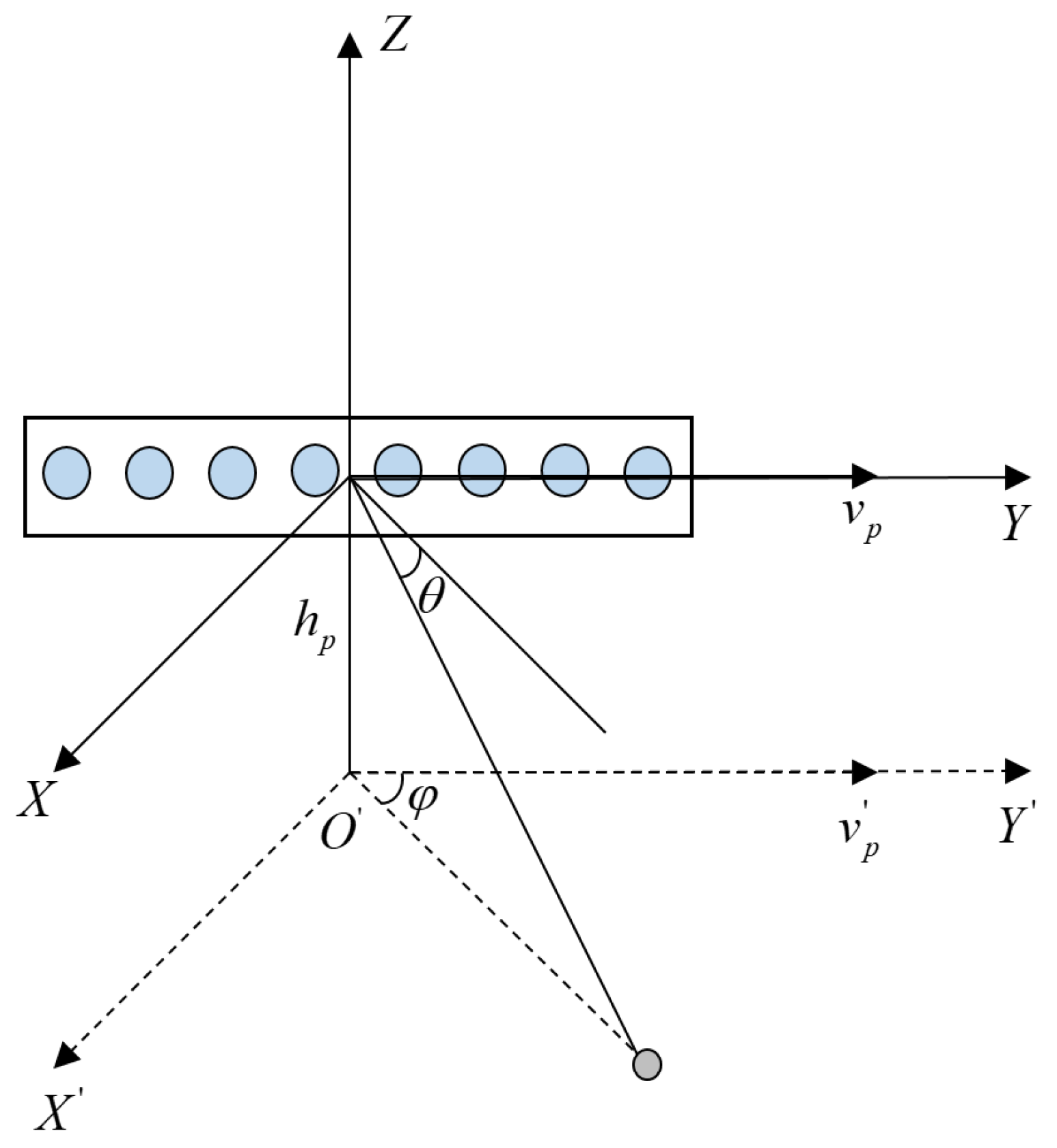
2. System Model and Derivation of Optimal Filters
3. Proposed MCV−STAP Algorithm and BAMCV−STAP Algorithm
3.1. Derivation of MCV
3.2. Proposed MCV−STAP Algorithm
| Algorithm 1 MCV−STAP algorithm. |
| Step1: Give initial values . |
| Step2: Sample from Equation (12) and sample from Equation (13). |
| Step3: For do |
| Calculate and via Equations (28) and (29); |
| Sample from Equation (20); |
| Calculate and via Equation (31); |
| Sample from Equation (30); |
| Calculate and via Equation (33); |
| Sample from Equation (32); |
| Check for convergence. |
| End For |
| Denote the last iter number as T. |
| Step4: Assume , calculate the CCM via Equation (8) and the space−time adaptive optimal |
| weight vector via Equation (1). |
| Step5: Denote the CUT as , the output of MCV−STAP algorithm solved by Gibbs sampling |
| is . |
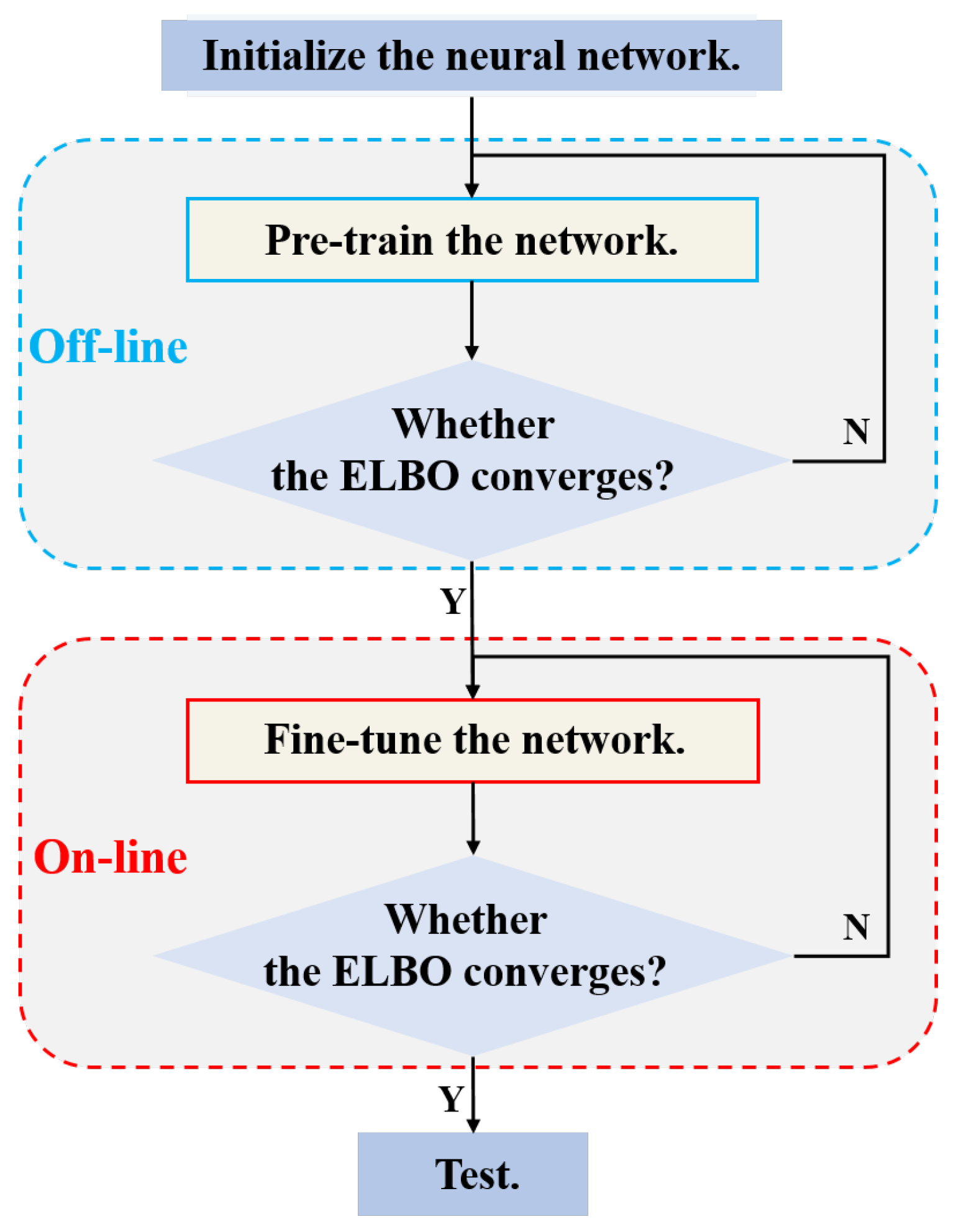
3.3. BAMCV−STAP Algorithm
| Algorithm 2 BAMCV−STAP algorithm. |
| Step1: Simulate data for pre−training using radar system parameters of realistic clutter data under |
| test. Denote the simulated dataset as and the realistic dataset as . |
| Step2: Pre−train the inference network with dataset off−line until the ELBO converges. |
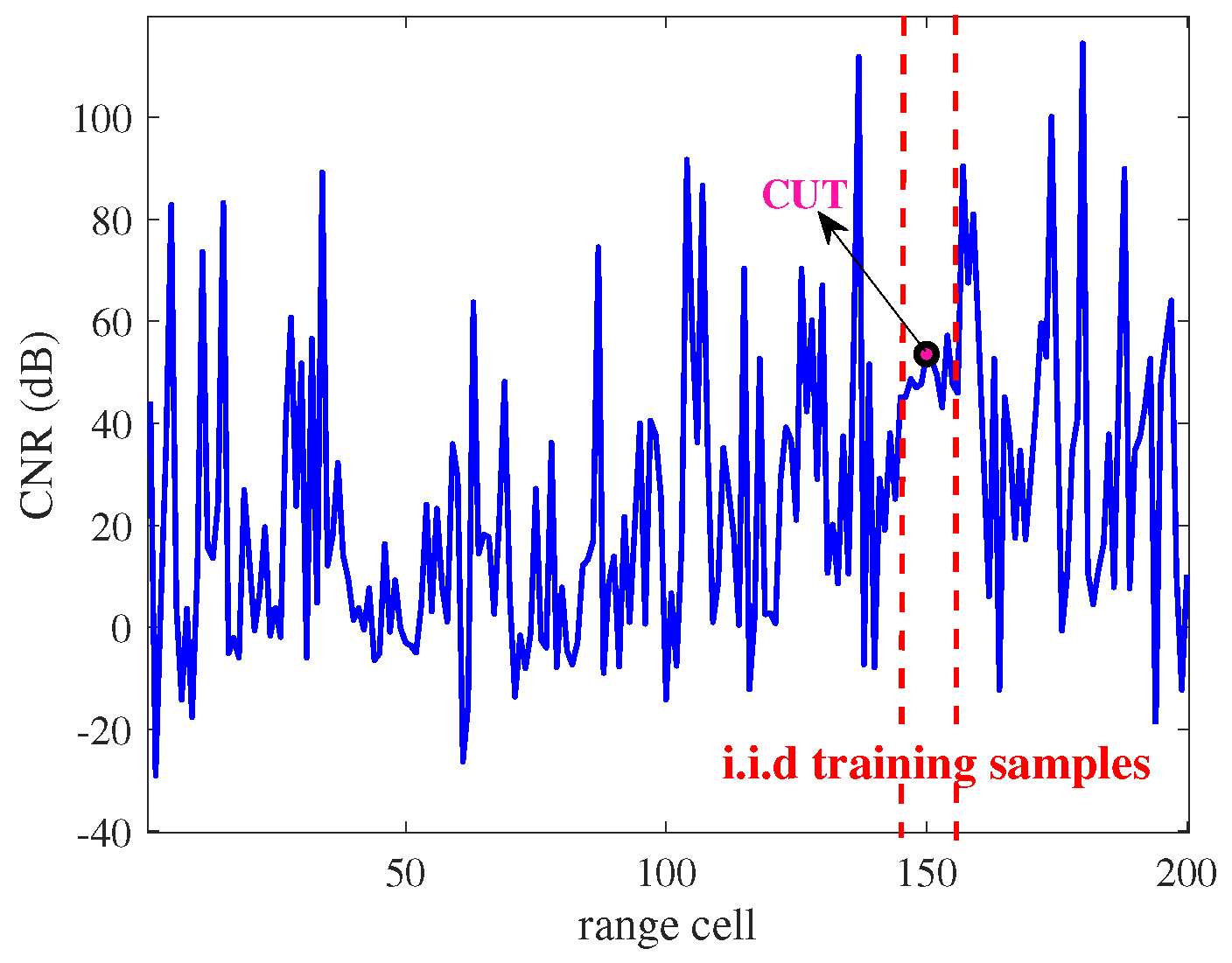
| Step3: Select CUT in and choose L training samples around CUT. |
| Step4: Fine−tune the inference network with the selected L training samples until the ELBO |
| converges again. Assume . |
| Step6: Estimate the CCM via Equation (8) and the space−time adaptive optimal weight vector via Equation (2). |
| Denote the weight vector as |
| Step7: Denote data in CUT as , the output of BAMCV−STAP solved by the inference network is |
| . |
- Decreasing the computational loads. Inspired by the gradient ascent scheme for parameters optimization, the parameters of BAMCV are updated by the backpropagation of the gradient, which only involves some linear operations, exponential operations and logarithmic operations, instead of involving complex inverse operations and multiple samplings appeared in MCV.
- Improving the convergence rate for testing. As the inference network is pre−trained off−line, only a few iterations are taken in BAMCV to obtain the recovery results of observations rather than a large number of time−consuming iterations per testing in MCV.
4. Numerical Results
4.1. Simulated Data
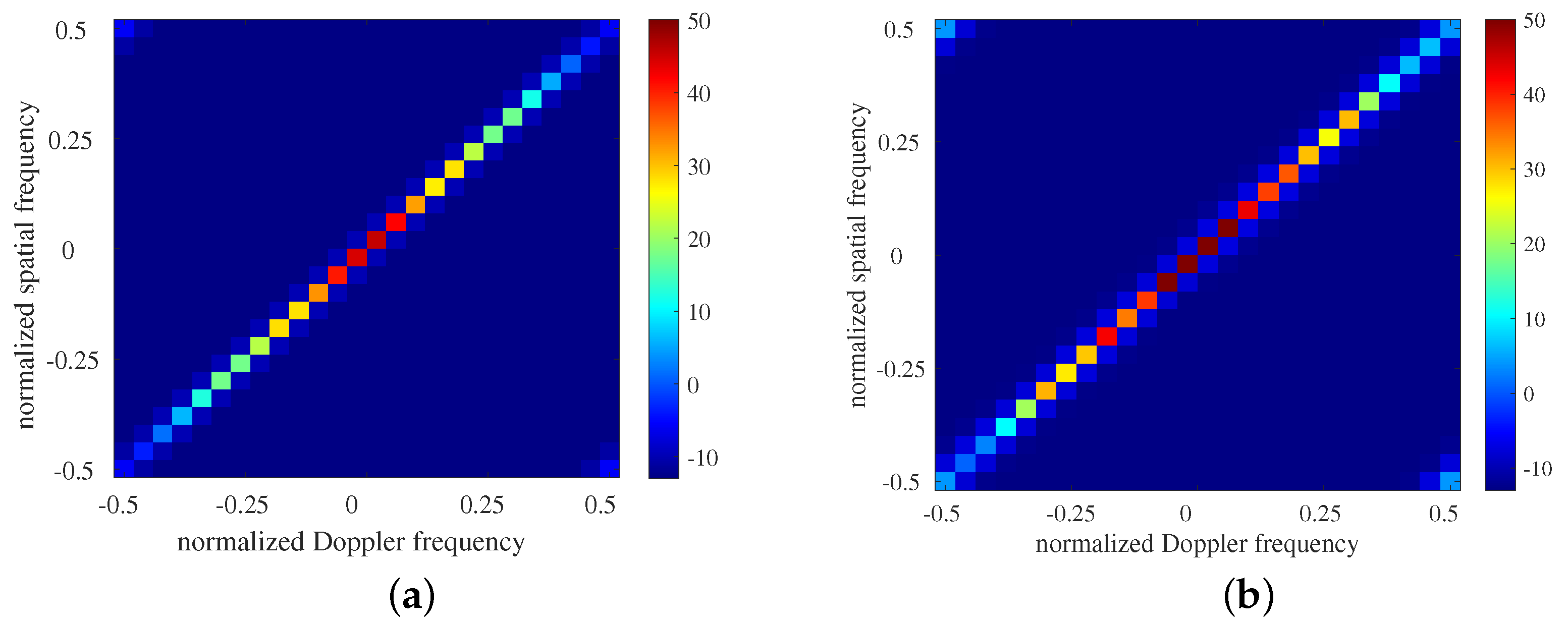
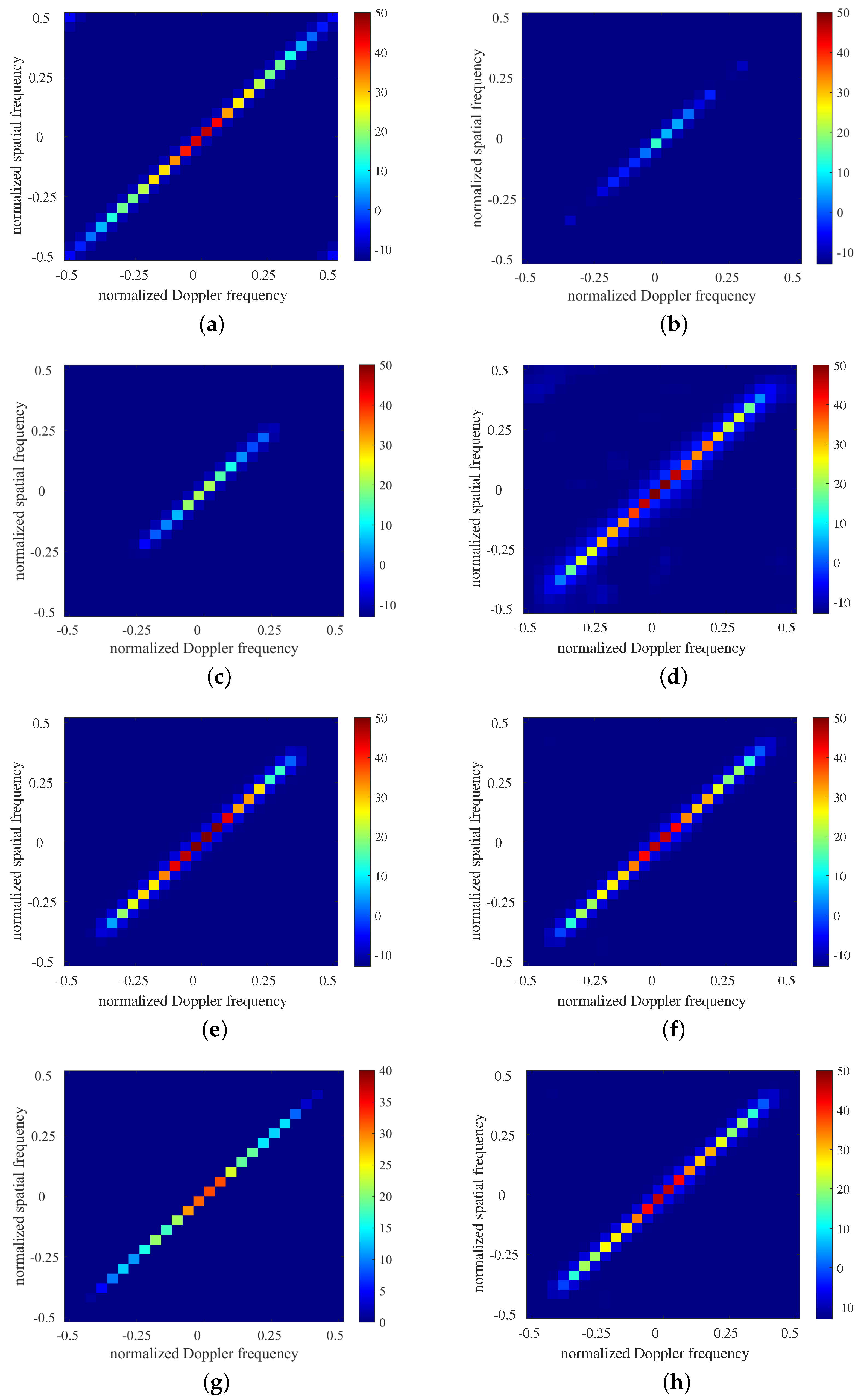
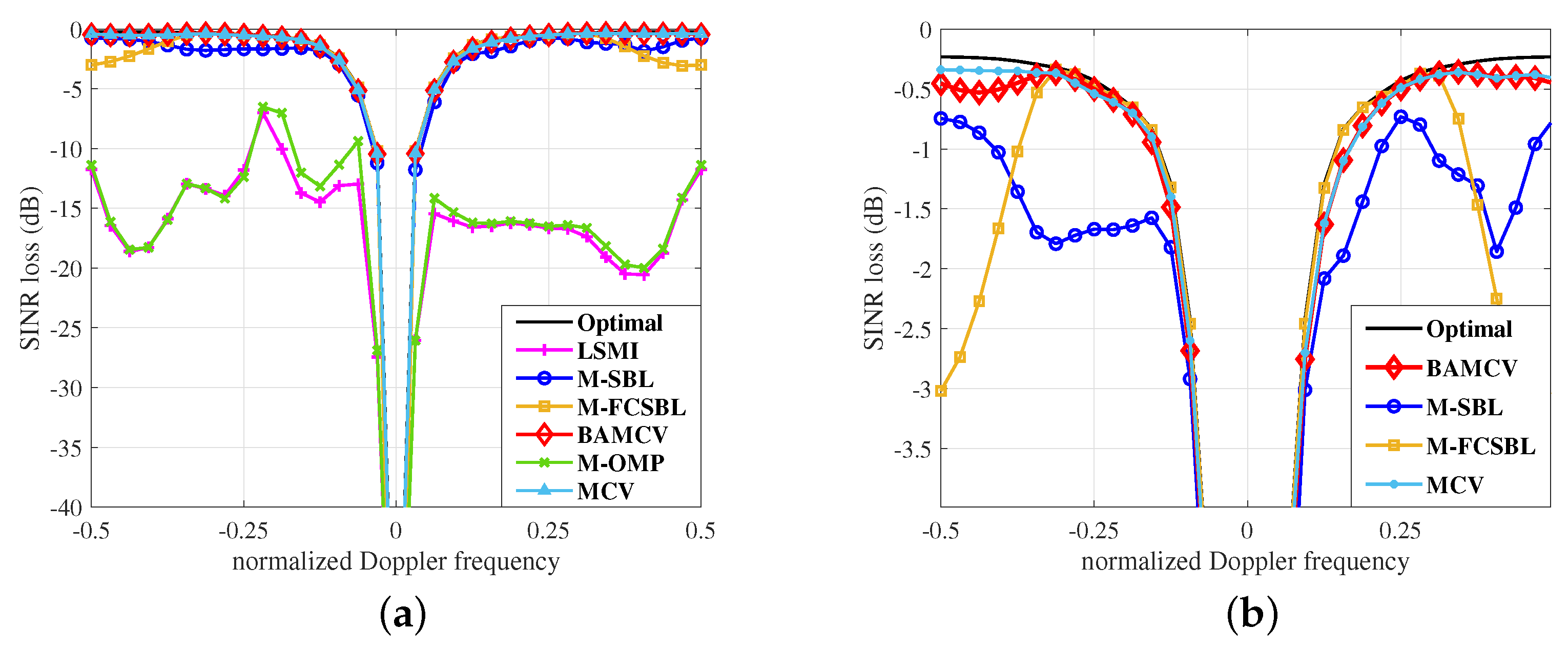
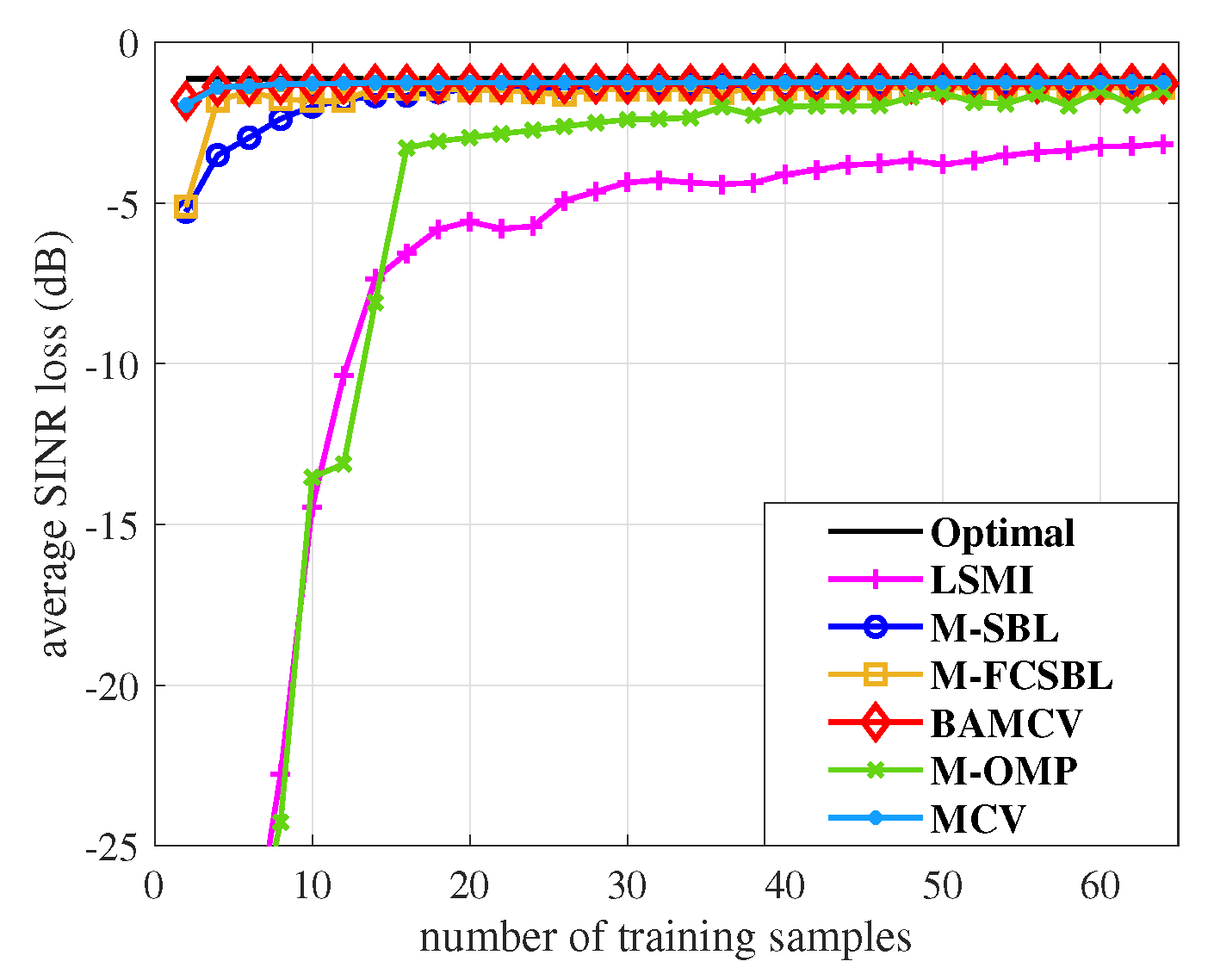
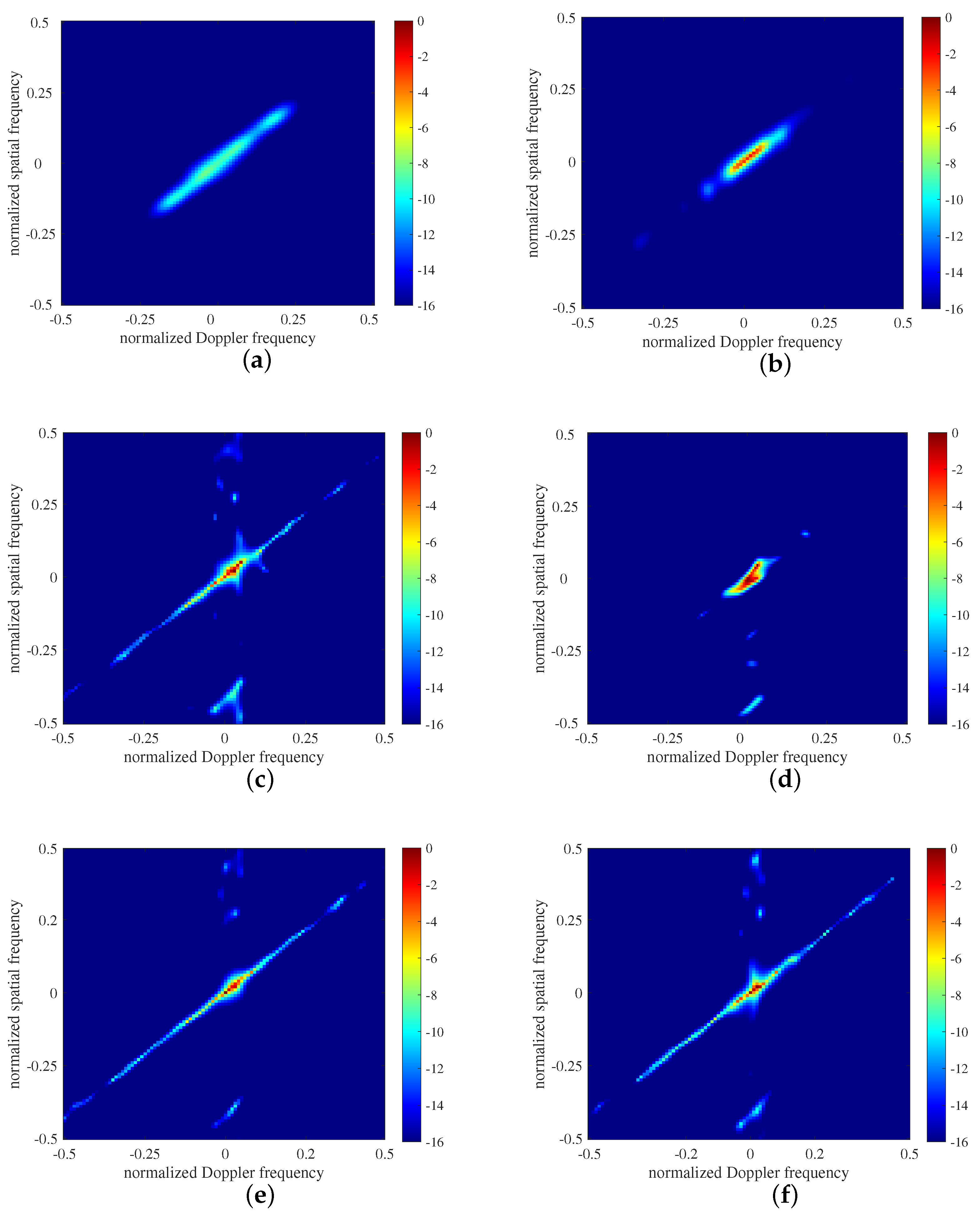
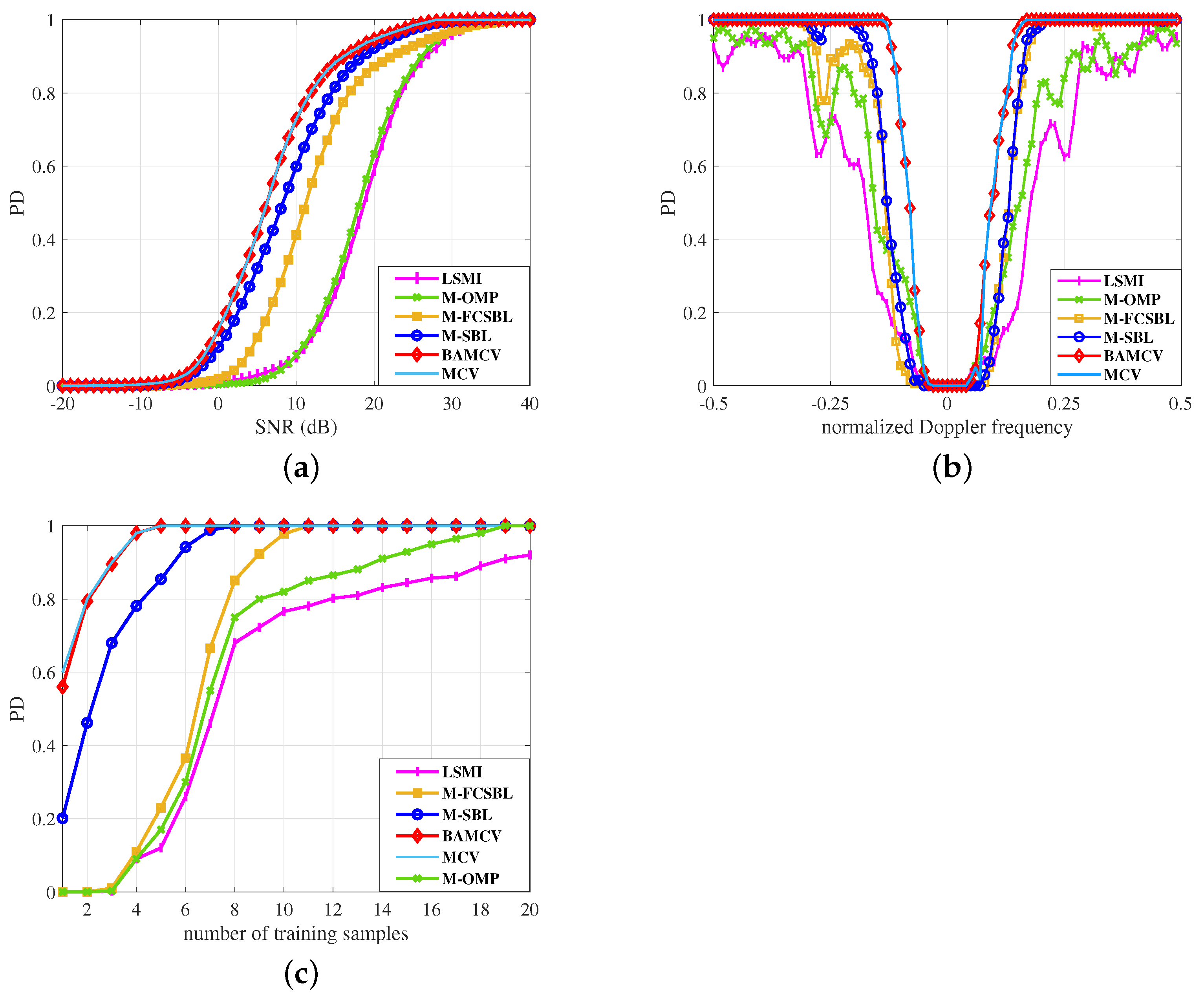
4.1.1. Analysis of Clutter Suppression Performance
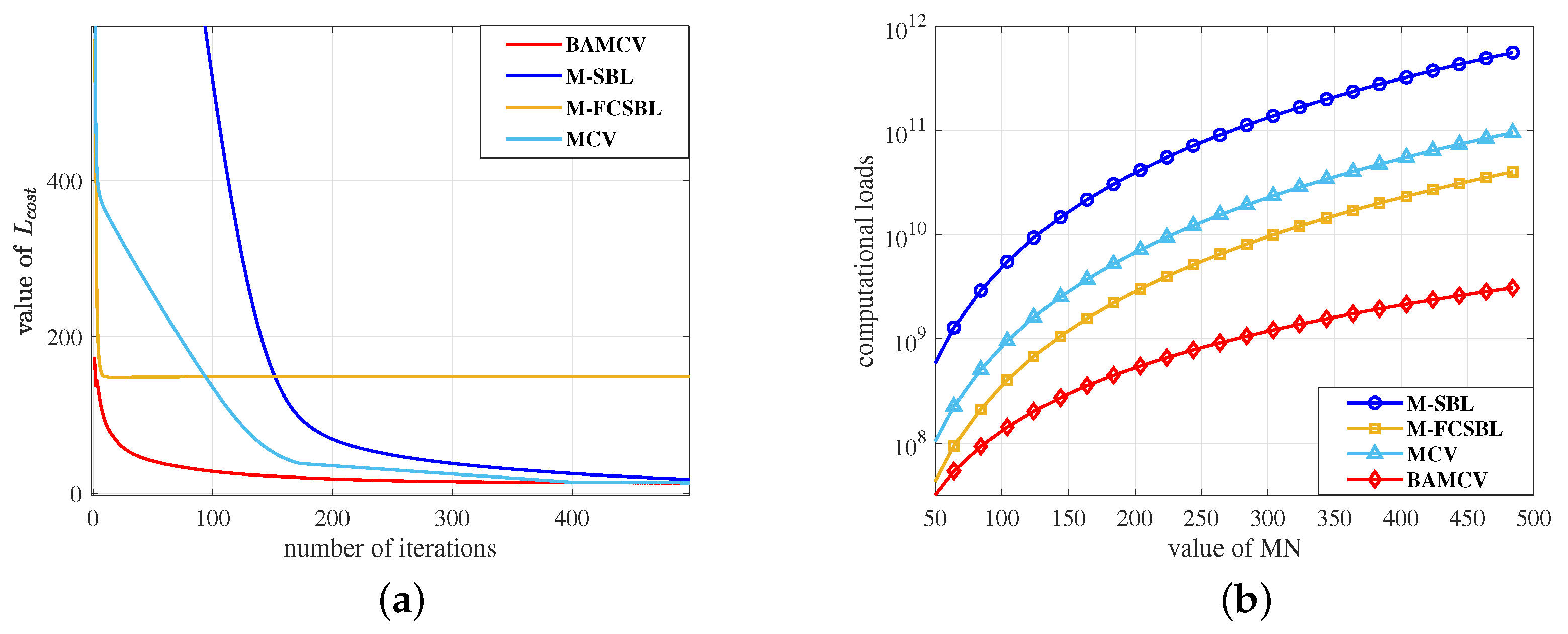
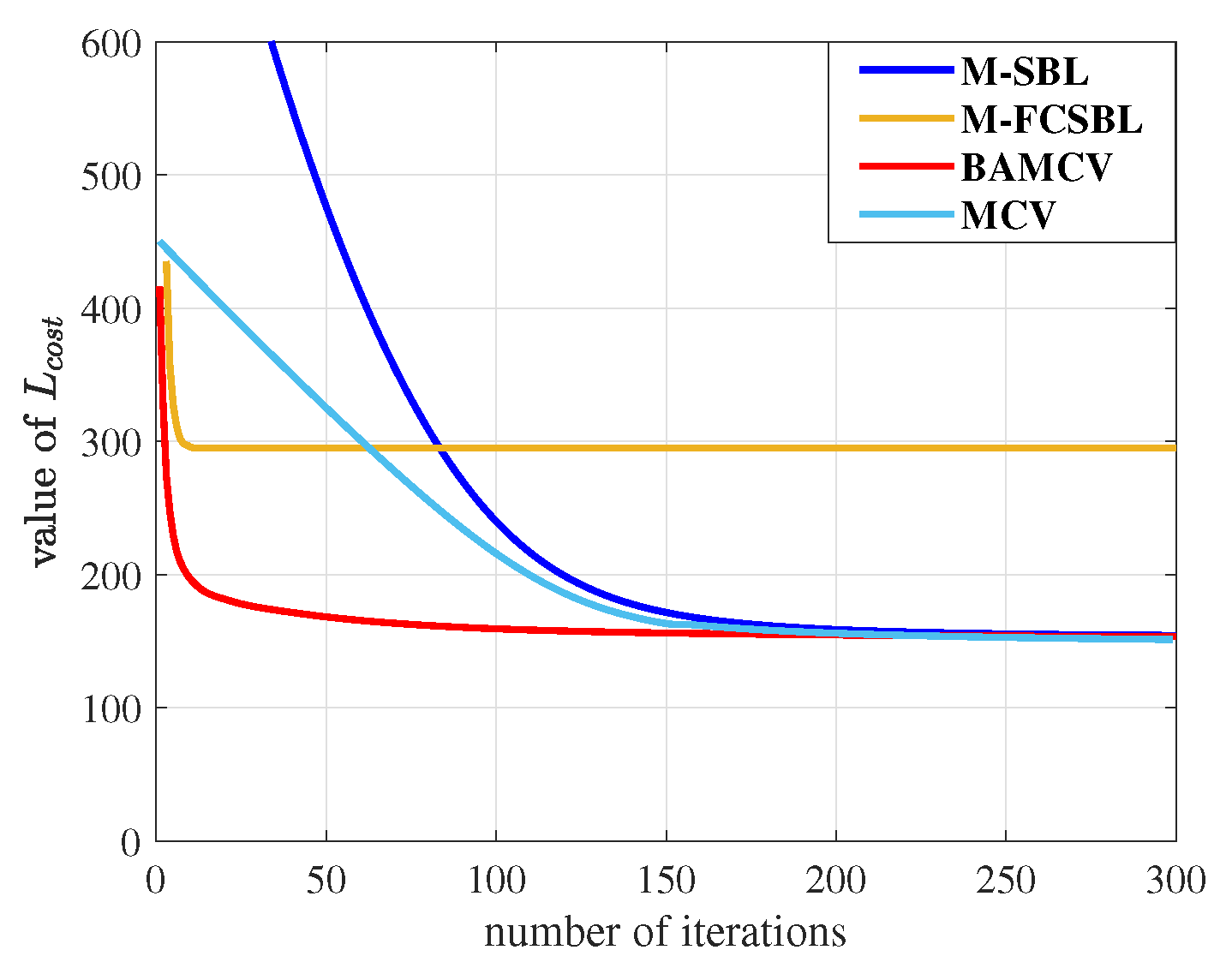
4.1.2. Analysis of Computational Loads and Convergence Rate
4.2. Measured Data
5. Discussion
6. Conclusions
Author Contributions
Funding
Data Availability Statement
Conflicts of Interest
References
- Chen, X.; Cheng, Y.; Wu, H.; Wang, H. Heterogeneous clutter suppression for airborne radar STAP based on matrix manifolds. Remote Sens. 2021, 13, 3195. [Google Scholar] [CrossRef]
- Li, H.; Liao, G.; Xu, J.; Zeng, C. Sub-CPI STAP based clutter suppression and target refocusing with airborne radar system. Digit. Signal Process. 2022, 123, 103418. [Google Scholar] [CrossRef]
- Liu, K.; Wang, T.; Wu, J.; Chen, J. A Two-Stage STAP Method Based on Fine Doppler Localization and Sparse Bayesian Learning in the Presence of Arbitrary Array Errors. Sensors 2022, 22, 77. [Google Scholar] [CrossRef] [PubMed]
- Xiao, H.; Wang, T.; Zhang, S.; Wen, C. A robust refined training sample reweighting space–time adaptive processing method for airborne radar in heterogeneous environment. IET Radar Sonar Nav. 2021, 15, 310–322. [Google Scholar] [CrossRef]
- Yifeng, W.; Tong, W.; Jianxin, W.; Jia, D. Robust training samples selection algorithm based on spectral similarity for space–time adaptive processing in heterogeneous interference environments. IET Radar Sonar Nav. 2015, 9, 778–782. [Google Scholar] [CrossRef]
- Liu, J.; Liu, W.; Liu, H. A simpler proof of rapid convergence rate in adaptive arrays. IEEE Trans. Aerosp. Electron. Syst. 2017, 53, 135–136. [Google Scholar] [CrossRef]
- Zhang, W.; He, Z.; Li, J.; Liu, H.; Sun, Y. A method for finding best channels in beam-space post-Doppler reduced-dimension STAP. IEEE Trans. Aerosp. Electron. Syst. 2014, 50, 254–264. [Google Scholar] [CrossRef]
- Zhang, W.; He, Z.; Li, J.; Li, C. Beamspace reduced-dimension space–time adaptive processing for multiple-input multiple-output radar based on maximum cross-correlation energy. IET Radar Sonar Nav. 2015, 9, 772–777. [Google Scholar] [CrossRef]
- Wang, X.; Yang, Z.; Huang, J.; de Lamare, R.C. Robust two-stage reduced-dimension sparsity-aware STAP for airborne radar With coprime arrays. IEEE Trans. Signal Process. 2020, 68, 81–96. [Google Scholar] [CrossRef]
- Zhang, W.; An, R.; He, N.; He, Z.; Li, H. Reduced dimension STAP based on sparse recovery in heterogeneous clutter environments. IEEE Trans. Aerosp. Electron. Syst. 2020, 56, 785–795. [Google Scholar] [CrossRef]
- Guerci, J.R.; Goldstein, J.S.; Reed, I.S. Optimal and adaptive reduced-rank STAP. IEEE Trans. Aerosp. Electron. Syst. 2000, 36, 647–663. [Google Scholar] [CrossRef]
- Fa, R.; de Lamare, R.C. Reduced-Rank STAP Algorithms using Joint Iterative Optimization of Filters. IEEE Trans. Aerosp. Electron. Syst. 2011, 47, 1668–1684. [Google Scholar] [CrossRef]
- Yang, Z.; Wang, X. Reduced-rank space-time adaptive processing algorithm based on multistage selections of angle-Doppler filters. IET Radar Sonar Nav. 2022, 16, 327–345. [Google Scholar] [CrossRef]
- Sarkar, T.K.; Wang, H.; Park, S.; Adve, R.; Koh, J.; Kim, K.; Zhang, Y.; Wicks, M.C.; Brown, R.D. A deterministic least-squares approach to space-time adaptive processing (STAP). IEEE Trans. Aerosp. Electron. Syst. 2001, 49, 91–103. [Google Scholar] [CrossRef] [Green Version]
- Guerci, J.R.; Baranoski, E.J. Knowledge-aided adaptive radar at DARPA: An overview. IEEE Signal Process. Mag. 2006, 23, 41–50. [Google Scholar] [CrossRef]
- Capraro, C.T.; Capraro, G.T.; Bradaric, I.; Weiner, D.D.; Wicks, M.C.; Baldygo, W.J. Implementing digital terrain data in knowledge-aided space-time adaptive processing. IEEE Trans. Aerosp. Electron. Syst. 2006, 42, 1080–1099. [Google Scholar] [CrossRef]
- Cui, N.; Xing, K.; Duan, K.; Yu, Z. Knowledge-aided block sparse Bayesian learning STAP for phased-array MIMO airborne radar. IET Radar Sonar Navig. 2021, 15, 1628–1642. [Google Scholar] [CrossRef]
- Liu, M.; Zou, L.; Yu, X.; Zhou, Y.; Wang, X.; Tang, B. Knowledge Aided Covariance Matrix Estimation via Gaussian Kernel Function for Airborne SR-STAP. IEEE Access 2020, 8, 5970–5978. [Google Scholar] [CrossRef]
- Zhu, X.; Li, J.; Stoica, P. Knowledge-aided space-time adaptive processing. IEEE Trans. Aerosp. Electron. Syst. 2011, 47, 1325–1336. [Google Scholar] [CrossRef]
- Yang, Z.; de Lamare, R.C.; Li, X. L1 regularized STAP algorithms With a generalized sidelobe canceler architecture for airborne radar. IEEE Trans. Signal Process. 2012, 60, 674–686. [Google Scholar] [CrossRef]
- Sun, K.; Zhang, H.; Li, G.; Meng, H.; Wang, X. A Novel STAP Algorithm using Sparse Recovery Technique. In Proceedings of the IEEE International Geoscience & Remote Sensing Symposium (IGARSS 2009), Cape Town, South Africa, 12–17 July 2009; pp. 336–339. [Google Scholar]
- Wu, Q.; Zhang, Y.D.; Amin, M.G.; Himed, B. Space-Time Adaptive Processing and Motion Parameter Estimation in Multistatic Passive Radar Using Sparse Bayesian Learning. IEEE Trans. Geosci. Remote Sens. 2016, 54, 944–957. [Google Scholar] [CrossRef]
- Yang, X.; Sun, Y.; Zeng, T.; Long, T.; Sarkar, T.K. Fast STAP Method Based on PAST with Sparse Constraint for Airborne Phased Array Radar. IEEE Trans. Signal Process. 2016, 64, 4550–4561. [Google Scholar] [CrossRef]
- Mallat, S.; Zhang, Z. Matching pursuits with time-frequency dictionaries. IEEE Trans. Signal Process. 1993, 41, 3397–3415. [Google Scholar] [CrossRef] [Green Version]
- Pati, Y.; Rezaiifar, R.; Krishnaprasad, P. Orthogonal matching pursuit: Recursive function approximation with applications to wavelet decomposition. In Proceedings of the 27th Asilomar Conference on Signals, Systems and Computers, Pacific Grove, CA, USA, 1–3 November 1993; pp. 40–44. [Google Scholar]
- Cotter, S.F.; Rao, B.D.; Engan, K.; Kreutz-Delgado, K. Sparse solutions to linear inverse problems with multiple measurement vectors. IEEE Trans. Signal Process. 2005, 53, 2477–2488. [Google Scholar] [CrossRef]
- Blumensath, T.; Davies, M.E. Gradient Pursuits. IEEE Trans. Signal Process. 2008, 56, 2370–2382. [Google Scholar] [CrossRef]
- Bruckstein, A.M.; Donoho, D.L.; Elad, M. From Sparse Solutions of Systems of Equations to Sparse Modeling of Signals and Images. SIAM Rev. 2009, 51, 34–81. [Google Scholar] [CrossRef] [Green Version]
- Tibshirani, R. Regression shrinkage and selection via the lasso: A retrospective. J. R. Stat. Soc. Series B Stat. Methodol. 2011, 73, 273–282. [Google Scholar] [CrossRef]
- Zibulevsky, M.; Elad, M. L1-L2 Optimization in Signal and Image Processing. IEEE Signal Process. Mag. 2010, 27, 76–88. [Google Scholar] [CrossRef]
- Chen, S.S.; Donoho, D.L.; Saunders, M.A. Atomic Decomposition by Basis Pursuit. SIAM Rev. 2001, 43, 129–159. [Google Scholar] [CrossRef] [Green Version]
- Wei, S.; Zhang, L.; Ma, H.; Liu, H. Sparse Frequency Waveform Optimization for High-Resolution ISAR Imaging. IEEE Trans. Geosci. Remote Sens. 2020, 58, 546–566. [Google Scholar] [CrossRef]
- Wu, Q.; Zhang, Y.D.; Amin, M.G.; Himed, B. Complex multitask Bayesian compressive sensing. In Proceedings of the IEEE International Conference on Acoustics, Speech and Signal Processing (ICASSP 2014), Florence, Italy, 4–9 May 2014; pp. 3375–3379. [Google Scholar]
- Wang, Z.; Xie, W.; Duan, K.; Wang, Y. Clutter suppression algorithm based on fast converging sparse Bayesian learning for airborne radar. Signal Process. 2017, 130, 159–168. [Google Scholar] [CrossRef]
- Poli, L.; Oliveri, G.; Viani, F.; Massa, A. MT–BCS-based microwave imaging approach through minimum-norm current expansion. IEEE Trans. Aerosp. Electron. Syst. 2013, 61, 4722–4732. [Google Scholar] [CrossRef]
- Tipping, M.E. Sparse Bayesian Learning and the Relevance Vector Machine. J. Mach. Learn. Res. 2001, 1, 211–244. [Google Scholar]
- Wipf, D.P.; Rao, B.D. An Empirical Bayesian Strategy for Solving the Simultaneous Sparse Approximation Problem. IEEE Trans. Signal Process. 2007, 55, 3704–3716. [Google Scholar] [CrossRef]
- Duan, K.; Chen, H.; Xie, W.; Wang, Y. Deep learning for high-resolution estimation of clutter angle-Doppler spectrum in STAP. IET Radar Sonar Nav. 2022, 16, 193–207. [Google Scholar] [CrossRef]
- Bishop, C.M.; Tipping, M.E. Variational Relevance Vector Machines. In Proceedings of the the 16th Conference in Uncertainty in Artificial Intelligence, Stanford University, Stanford, CA, USA, 30 June–3 July 2000; pp. 46–53. [Google Scholar]
- Kingma, D.P.; Welling, M. Auto-Encoding Variational Bayes. In Proceedings of the International Conference on Learning Representations (ICLR 2014), Banff, AB, Canada, 14–16 April 2014. [Google Scholar]
- Notin, P.; Hernández-Lobato, J.M.; Gal, Y. Improving black-box optimization in VAE latent space using decoder uncertainty. In Proceedings of the Neural Information Processing Systems 2021 (NeurIPS 2021), Virtual, 6–14 December 2021; pp. 802–814. [Google Scholar]
- Zhou, Y.; Liang, X.; Zhang, W.; Zhang, L.; Song, X. VAE-based Deep SVDD for anomaly detection. Neurocomputing 2021, 453, 131–140. [Google Scholar] [CrossRef]
- Ding, M. The road from MLE to EM to VAE: A brief tutorial. AI Open 2022, 3, 29–34. [Google Scholar] [CrossRef]
- Hussain, A.; Anjum, U.; Channa, B.A.; Afzal, W.; Hussain, I.; Mir, I. Displaced Phase Center Antenna Processing For Airborne Phased Array Radar. In Proceedings of the 2021 International Bhurban Conference on Applied Sciences and Technologies (IBCAST), Islamabad, Pakistan, 12–16 January 2021; pp. 988–992. [Google Scholar]
- Ward, J. Space-time adaptive processing for airborne radar. In Proceedings of the 1995 International Conference on Acoustics, Speech, and Signal Processing, ICASSP, Detroit, MI, USA, 8–12 May 1995; pp. 2809–2812. [Google Scholar]
- Wipf, D.; Nagarajan, S. A New View of Automatic Relevance Determination. In Proceedings of the Twentieth Annual Conference On Neural Information Processing Systems (NIPS 2007), Vancouver, BC, Canada, 4–7 December 2006; Platt, J., Koller, D., Singer, Y., Roweis, S., Eds.; Curran Associates, Inc.: West Chester, PA, USA, 2007; Volume 20. [Google Scholar]
- Berger, J.O. Statistical Decision Theory and Bayesian Analysis, 2nd ed.; Springer: Berlin/Heidelberg, Germany, 1985. [Google Scholar]
- Jordan, M.I.; Ghahramani, Z.; Jaakkola, T.S.; Saul, L.K. An Introduction to Variational Methods for Graphical Models. Mach. Learn. 1999, 37, 183–233. [Google Scholar] [CrossRef]
- Worley, B. Scalable Mean-Field Sparse Bayesian Learning. IEEE Trans. Signal Process. 2019, 67, 6314–6326. [Google Scholar] [CrossRef]
- Tzikas, D.G.; Likas, A.C.; Galatsanos, N.P. The variational approximation for Bayesian inference. IEEE Signal Process. Mag. 2008, 25, 131–146. [Google Scholar] [CrossRef]
- Kingma, D.P.; Welling, M. Stochastic gradient VB and the variational auto-encoder. In Proceedings of the the 2rd International Conference on Learning Representations (ICLR 2014), London, UK, 8–9 July 2014; Volume 19, p. 121. [Google Scholar]
- Ruiz, F.J.R.; Titsias, M.K.; Blei, D.M. The Generalized Reparameterization Gradient. In Proceedings of the the 29th Annual Conference on Neural Information Processing Systems (NIPS 2016), Barcelona, Spain, 5–10 December 2016; pp. 460–468. [Google Scholar]
- Zhang, H.; Chen, B.; Guo, D.; Zhou, M. WHAI: Weibull Hybrid Autoencoding Inference for Deep Topic Modeling. In Proceedings of the the 6th International Conference on Learning Representations (ICLR 2018), Vancouver, BC, Canada, 30 April–3 May 2018. [Google Scholar]
- Duan, Z.; Wang, D.; Chen, B.; Wang, C.; Chen, W.; Li, Y.; Ren, J.; Zhou, M. Sawtooth Factorial Topic Embeddings Guided Gamma Belief Network. In Proceedings of the the 38th International Conference on Machine Learning (ICML 2021), Virtual Event, 18–24 July 2021; pp. 2903–2913. [Google Scholar]
- Hendrycks, D.; Lee, K.; Mazeika, M. Using Pre-Training Can Improve Model Robustness and Uncertainty. In Proceedings of the the 36th International Conference on Machine Learning (ICML 2019), Long Beach, CA, USA, 9–15 June 2019; pp. 2712–2721. [Google Scholar]
- Robey, F.; Fuhrmann, D.; Kelly, E.; Nitzberg, R. A CFAR adaptive matched filter detector. IEEE Trans. Aerosp. Electron. Syst. 1992, 28, 208–216. [Google Scholar] [CrossRef] [Green Version]
- Carlson, B. Covariance matrix estimation errors and diagonal loading in adaptive arrays. IEEE Trans. Aerosp. Electron. Syst. 1988, 24, 397–401. [Google Scholar] [CrossRef]
- Cox, H.; Zeskind, R.M.; Owen, M.M. Robust adaptive beamforming. IEEE Trans. Acoust. Speech Signal Process. 1987, 35, 1365–1376. [Google Scholar] [CrossRef] [Green Version]
- Chen, J.; Huo, X. Theoretical Results on Sparse Representations of Multiple-Measurement Vectors. IEEE Trans. Signal Process. 2006, 54, 4634–4643. [Google Scholar] [CrossRef] [Green Version]
- Kingma, D.P.; Ba, J. Adam: A Method for Stochastic Optimization. In Proceedings of the the 3rd International Conference on Learning Representations (ICLR 2015), San Diego, CA, USA, 7–9 May 2015. [Google Scholar]
- Little, M.; Perry, W. Real-time multichannel airborne radar measurements. In Proceedings of the the 1997 IEEE National Radar Conference, Syracuse, NY, USA, 13–15 May 1997; pp. 138–142. [Google Scholar]


| Parameters | Dimensions | Parameters | Dimensions | Parameters | Dimensions |
|---|---|---|---|---|---|
| Performance Metric | Simulated Data | Measured Data | |
|---|---|---|---|
| Clutter Suppression | SINR loss | √ | |
| PD | √ | ||
| Real−time Processing | Convergence rate | √ | √ |
| Computational loads | √ | √ |
| Parameters | Value | Parameters | Value |
|---|---|---|---|
| Carrier frequency (Hz) | 1.25 G | Platform velocity (m/s) | 125 |
| Bandwidth (Hz) | 2.5 M | Platform height (m) | 6000 |
| Mainbeam azimuth (∘) | 0 | Pulse number in one CPI | 8 |
| Mainbeam elevation (∘) | 0 | Antenna elements number | 8 |
| Pulse repetition frequency (Hz) | 2000 | Range cell number | 400 |
| True Noise Power | M−SBL | M−FCSBL | MCV | BAMCV |
|---|---|---|---|---|
| 0.01 | 0.0111 | 0.00973 | 0.0101 | |
| 0.1 | 0.1197 | 0.1061 | 0.1103 | |
| 1 | 1.0117 | 0.9937 | 0.9925 | |
| 5 | 4.7692 | 4.9793 | 4.9001 | |
| 10 | 11.1382 | 9.9992 | 9.9856 |
| Approach | Running Time Per Iteration (s) |
|---|---|
| M−SBL | |
| M−FCSBL | |
| MCV | |
| BAMCV |
| Approach | Computational Loads |
|---|---|
| M−SBL | |
| M−FCSBL | |
| MCV | |
| BAMCV |
| Parameters | Value | Parameters | Value |
|---|---|---|---|
| Pulse repetition frequency (Hz) | 1984 | Antenna array spacing of azimuth (m) | 0.1029 |
| Wavelength (m) | 0.24 | Antenna array spacing of elevation (m) | 0.5629 |
| Pulse number in one CPI | 128 | Platform height (m) | 10,188 |
| Antenna elements number of azimuth | 11 | Range cell number | 400 |
| Antenna elements number of elevation | 2 |
| Approach | Running Time Per Iteration (s) |
|---|---|
| M−SBL | |
| M−FCSBL | |
| MCV | |
| BAMCV |
Publisher’s Note: MDPI stays neutral with regard to jurisdictional claims in published maps and institutional affiliations. |
© 2022 by the authors. Licensee MDPI, Basel, Switzerland. This article is an open access article distributed under the terms and conditions of the Creative Commons Attribution (CC BY) license (https://creativecommons.org/licenses/by/4.0/).
Share and Cite
Zhang, C.; Zhao, H.; Chen, W.; Chen, B.; Wang, P.; Jia, C.; Liu, H. Robust Multiple-Measurement Sparsity-Aware STAP with Bayesian Variational Autoencoder. Remote Sens. 2022, 14, 3800. https://doi.org/10.3390/rs14153800
Zhang C, Zhao H, Chen W, Chen B, Wang P, Jia C, Liu H. Robust Multiple-Measurement Sparsity-Aware STAP with Bayesian Variational Autoencoder. Remote Sensing. 2022; 14(15):3800. https://doi.org/10.3390/rs14153800
Chicago/Turabian StyleZhang, Chenxi, Huiliang Zhao, Wenchao Chen, Bo Chen, Penghui Wang, Changrui Jia, and Hongwei Liu. 2022. "Robust Multiple-Measurement Sparsity-Aware STAP with Bayesian Variational Autoencoder" Remote Sensing 14, no. 15: 3800. https://doi.org/10.3390/rs14153800
APA StyleZhang, C., Zhao, H., Chen, W., Chen, B., Wang, P., Jia, C., & Liu, H. (2022). Robust Multiple-Measurement Sparsity-Aware STAP with Bayesian Variational Autoencoder. Remote Sensing, 14(15), 3800. https://doi.org/10.3390/rs14153800