Article

Soil Moisture Mapping with Moisture-Related Indices, OPTRAM, and an Integrated Random Forest-OPTRAM Algorithm from Landsat 8 Images

1
CFAES Rattan Lal Center for Carbon Management and Sequestration, The Ohio State University, Columbus, OH 43210, USA
2
Department of Soil Science, School of Natural Resources Sciences, North Dakota State University, Fargo, ND 58102, USA
3
Department of Geoscience, North Dakota State University, Fargo, ND 58102, USA
*
Author to whom correspondence should be addressed.
Remote Sens. 2022, 14(15), 3801; https://doi.org/10.3390/rs14153801
Submission received: 16 June 2022 / Revised: 29 July 2022 / Accepted: 4 August 2022 / Published: 6 August 2022
(This article belongs to the Section Remote Sensing in Agriculture and Vegetation)

Abstract

:
Remote sensing tools have been extensively used for large-scale soil moisture (SM) mapping in recent years, using Landsat satellite images. Rainfall, soil clay percentage, and the standardized precipitation index play key roles in determining the moisture content of crop fields. The objective of this study was to (i) calculate and determine the effectiveness of moisture-related indices in predicting surface SM, (ii) predict surface SM from satellite images using the Optical Trapezoid Model (OPTRAM), and (iii) evaluate if the OPTRAM predictions can be improved by incorporating weather station, soil, and crop data with a random forest algorithm. The ENVI® platform was used to create moisture-related indices maps, and the Google Earth Engine (GEE) was used to prepare OPTRAM maps. The results showed a very weak relationship between the moisture-related indices and surface SM content where r2 and slopes were ˂0.10 and ˂0.20, respectively. OPTRAM SM, when compared with in situ surface moisture, showed weak relationship with regression values ˂0.2. Surface SM was then predicted using random forest regression using OPTRAM moisture values, rainfall, and the standardized precipitation index (SPI), and percent clay showed high goodness of fit (r2 = 0.69) and low root mean square error (RMSE = 0.053 m3 m−3).

1. Introduction

Remote sensing has been used as an advance tool for agricultural interpretation [1]. A prime area of research in agriculture is the in-field variability of plant water stress across large scales, which directly relates to in-field SM [2]. Estimation of surface SM provides farmers with key information on water stress, which aids crop yield projections, assessments of drought and excessive water conditions, and informs water management practices (e.g., irrigation, drainage) [3,4]. Remote sensing can be effectively used to estimate SM because soil optical reflection and thermal emissions are highly correlated with SM [5,6]. Remotely sensed visible and thermal infrared wavelengths provide more information when combined, rather than on their own [7]. However, spatial and temporal information are needed to produce precise and accurate estimates [6]. Remote sensing techniques provide tools for mapping SM at large spatial and temporal scales [8]. Several mathematical models using remotely sensed data have been developed to estimate SM using satellite optical image datasets, such as Landsat and sentinel, that are freely available. Remote sensing provides time and cost-effective data, which are valuable for SM estimation at the regional and national levels, using various techniques [9,10,11]. There are numerous methods used in remote sensing to estimate SM. All these methods are based on the type of image used, such as microwaves [12], thermal, visible, and infrared [13], radiometric behavior of infrared waves [14], and the use of relationships between surface temperature and fractional vegetation cover to estimate SM [15]. Vegetation indices can be misleading for estimating SM due to the time lag between changes in SM and corresponding changes in the vegetation indices [16,17].

1.1. Moisture-Related Indices

One common approach to estimate SM across landscapes has been to derive moisture from proxy measurements like moisture-related indices derived from satellite imagery. For instance, investigators have used reflectance data, such as the Normalized Difference Vegetation Index (NDVI) [18] and Normalized Difference Water Index (NDWI) [19], to estimate SM by the greenness and water content in the leaves of crop canopies. NDVI is a routinely produced and used product for indicating vegetation water content, SM, and crop yield prediction. NDVI has limitations for estimating SM because each crop species has its own unique relation with chlorophyll content, and a decrease in chlorophyll does not imply low SM [20]. Jackson et al. [21] found NDWI to be a superior index to NDVI for estimating SM. For example, in maize, they reported that NDVI and NDWI have a root mean square error (RMSE) of 0.735 and 0.576 kg m−2 with a bias of 0.336 and −0.010 kg m−2, respectively. Similarly, in soybean, a RMSE of 0.203 and 0.171 kg m−2 with a bias of 0.071 and −0.015 kg m−2 were observed for NDVI and NDWI, respectively. NDWI determines the water volume per leaf, which mostly depends on the leaf area index and crop canopy, and not necessarily the SM content. Other moisture-related indices such as the Normalized Difference Moisture Index (NDMI), Enhanced Vegetation Index (EVI), Atmospherically Resistant Vegetation Index (ARVI), and Structure Insensitive Pigment Index (SIPI) have been used to established relationships with SM using different bands (green, blue, red, infrared, short-wave infrared). Owe et al. [22] found incorporation of the vegetative index (NDVI) parameter calculated using Advanced Very High-Resolution Radiometer (AVHRR) from the NOAA-7 satellite improved the model for approximately 70% of variability in modeled surface soil moisture. NDVI derived from NOAA-AVHRR satellite data was well-correlated with simulated soil water (r2 = 0.64) for agricultural and pastureland use [23]. These indices have been successful in some region-specific cases, but not generally across all cases, and they lack wide application [21].

1.2. Physically Based Models

Physically based models are commonly preferred over the empirical moisture-related indices, but they also have their own limitations due to various confounding factors and the need for specific parameters. For instance, land surface temperature (LST) has been used as key parameter that relates with surface energy and water balance at local and large scales and helps in monitoring climate, vegetation, and hydrological cycles [24]. Energy is exchanged between land surface and atmosphere when SM evaporates into atmosphere. This demonstrates that SM not only depends on rainfall but also on soil surface temperature. The triangle (NDVI-LST) method is a widely used model [25,26,27] for estimating SM, but it has two major limitations. The first limitation is the requirement of thermal data, which is not applicable to all types of satellite images. The second limitation is that LST is affected by wind speed, air temperature, and humidity.
To overcome these two limitations, Sadeghi et al. [28] proposed the physically based Optical Trapezoidal Model (OPTRAM) for SM estimation. This model uses Short Wave Infrared (SWIR) transformed reflectance (STR) instead of LST. This results in the STR-NDVI space remaining nearly time invariant because reflectance is a function of only the surface properties and not the ambient atmospheric condition as LST. The OPTRAM model forms a trapezoid space using both NDVI as a measure of vegetative fraction and the STR to establish the linear relationship for dry and wet edges, which helps to estimate SM. STR does not significantly change with ambient atmospheric condition and can be universally parameterized for a given location. The combination of moisture-related indices and STR can provide useful information for the detection of spatial and temporal distributions of SM. Additionally, researchers have used historical meteorological records to develop time-invariable coefficients, which are used with remote sensing data such as LST and STR to estimate SM [29]. This is important in improving the spatial and temporal resolution of surface SM information for precision agriculture. There is great potential of using optical/thermal satellite images and meteorological data to develop an all-weather SM model [30].
However, SM mapping using satellite image processing may not provide accurate values in all cases, because field SM is dependent on a suite of complex factors (canopy, crop type and growth stage, crop residue, soil type). In addition to field conditions, rainfall is another important factor affecting SM content. There has been significant work on establishing a relation between rainfall and SM, so that rainfall data can be used to predict SM [31,32]. Brocca et al. [33] found four-day cumulative rainfall can be effectively used to predict SM with correlation coefficient values of 0.8 and a root mean square error (RMSE) of 1.36 mm day-1. Standardized Precipitation Index (SPI) is used to measure precipitation change over time at different time scale levels (1, 3, 6, 12 months) and is a valuable tool for indicating meteorological drought using past rainfall patterns.

1.3. Potential for Machine Learning to Overcome Challenges with OPTRAM

Despite the progress in estimating high-resolution SM across large areas, an integrated approach to predicting SM with the use of meteorological data, crop and field data, and remote sensing images has been lacking [34]. Additionally, some studies have reported poor performance of the OPTRAM model for specific regions. For instance, Babaeian et al. [35] observed r2 values from 0.01 to 0.49 and RMSE ranges from 0.05 to 0.08 m3 m−3 SM in the United States. Yadav et al. [36] reported accuracies of less than 10% when compared with other models (thermal) for the Lalitpur district of India. Yadav et al. [36] concluded that this reduced accuracy might be due to the lack of penetration of optical bands in the fully or densely covered vegetation. Similarly, Chen et al. [37] evaluated OPTRAM SM estimates using MODIS data and observed r2 values of 0.10 to 0.50 with RMSE’s from 0.05 to 0.13 m3 m−3, respectively. They suggested that the poor performance between the OPTRAM SM estimates and in situ SM might be due to rough image resolution and heterogenous terrains [37].
These studies characterized the spatial distribution of surface SM solely by using remote sensing. Very few studies have been conducted to incorporate climatic conditions and geographical or field and crop characteristics [38]. As part of the surface–atmosphere energy flux, parameters such as precipitation, LST, and ET can substantially modify SM across the landscape [39,40]. Recently, machine learning techniques have become useful for predicting SM under different field conditions. Machine learning techniques have the advantage and ability to learn and approximate complex non-linear mapping while requiring no assumptions on the distribution of the data. Machine learning techniques can also integrate data from different sources with poorly defined or unknown probability density functions [41]. For example, Ali et al. [41] and Paloscia et al. [42] showed machine learning techniques (e.g., Artificial Neural Network, Support Vector Regression) can outperform other parametric approaches for estimating SM and improved their performance with an increasing number of observed datasets. Therefore, integrating meteorological data from weather Mesonet and field characteristics (soil and crop data) along with OPTRAM SM values in a machine learning algorithm has the potential to be a valuable tool in mapping high-resolution SM across large areas.

1.4. Study Objectives

The objectives of this study were to (1) calculate and determine the effectiveness of moisture-related indices in predicting surface SM, (2) predict surface SM from the satellite images using OPTRAM, and (3) evaluate if the OPTRAM predictions can be improved by incorporating weather station, soil, and crop data with a random forest machine learning algorithm.

2. Materials and Methods
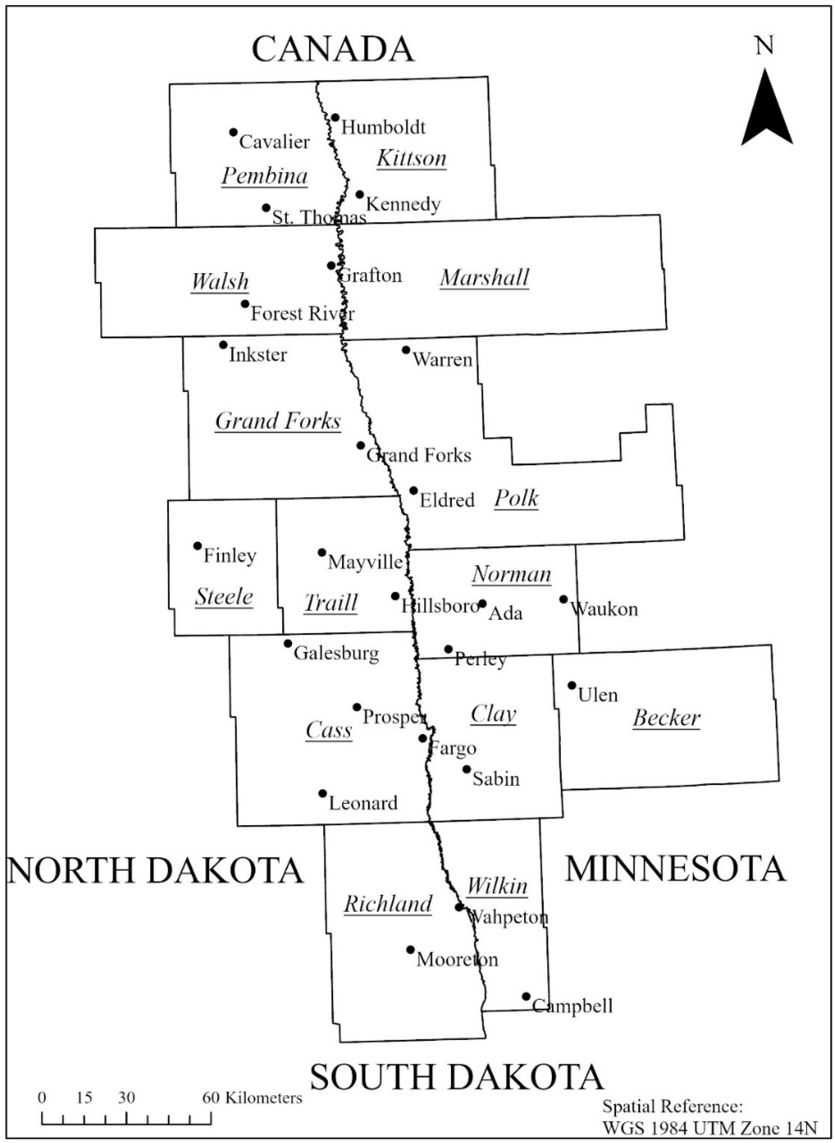
2.1. Study Area

The study area covered eight counties of North Dakota and seven counties of Minnesota that lie on either side of the Red River of the North (Latitude = 45.96 to 48.99 and Longitude = −95.51 to −98.01). Surface SM was collected for 2019 crop growing season. Maize (Zea mays L.), soybean (Glycine max (L.) Merr.), wheat (Triticum aestivum L.), barley (Hordeum vulgare L.), sugar beet (Beta vulgaris), canola (Brassica napus), sunflower (Helianthus annuus L.), potato (Solanum tuberosum L.), dry beans (Phaseolus vulgaris), and oats (Avena sativa L.) are major crops grown in the Red River Valley of the North (RRVN). Twenty-five weather stations (NDAWN, 2020) distributed across counties of MN (n = 10) and ND (n = 15) were selected for this study, which covers the RRVN (Figure 1).

2.2. Field Data Collection

Soil samples were collected from the twenty-five weather stations and three adjacent crop fields within 2 km of each weather station (i.e., 100 sample collection sites). Samples from all 100 collection sites were obtained at 16-day intervals, coinciding with the Landsat 8 satellite passing days (18 June to 29 September 2019). The adjacent crop fields near the weather stations were planted with soybean (n = 24), wheat (n = 18), corn (n = 16), sugar beet (n = 6), dry beans (n = 5), oats (n = 2), barley (n = 1), potato (n = 1), canola (n = 1), and alfalfa (n = 1). At each collection site, three composite soil samples (0–6 cm) were collected and averaged to get a representative surface SM. Gravimetric water content was calculated using the oven drying method, and volumetric water content (VWC) was determined by multiplying the bulk density with the gravimetric water content [43]. The growth stages of the crops were monitored following the standard methods established by the United States Department of Agriculture [44] for each cropped field and recorded every 16 days.

2.3. Satellite Image Processing

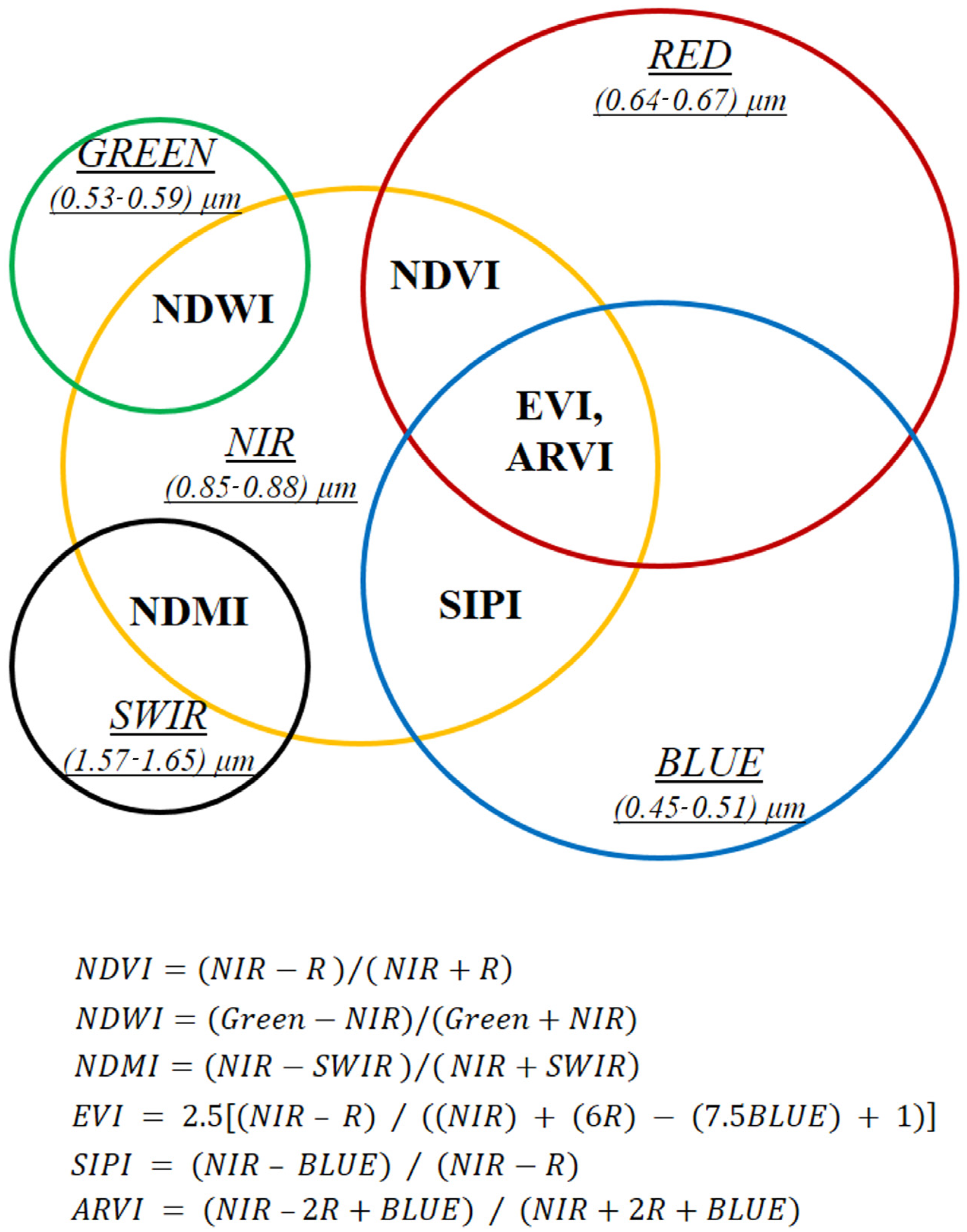
2.3.1. Moisture-Related Indices
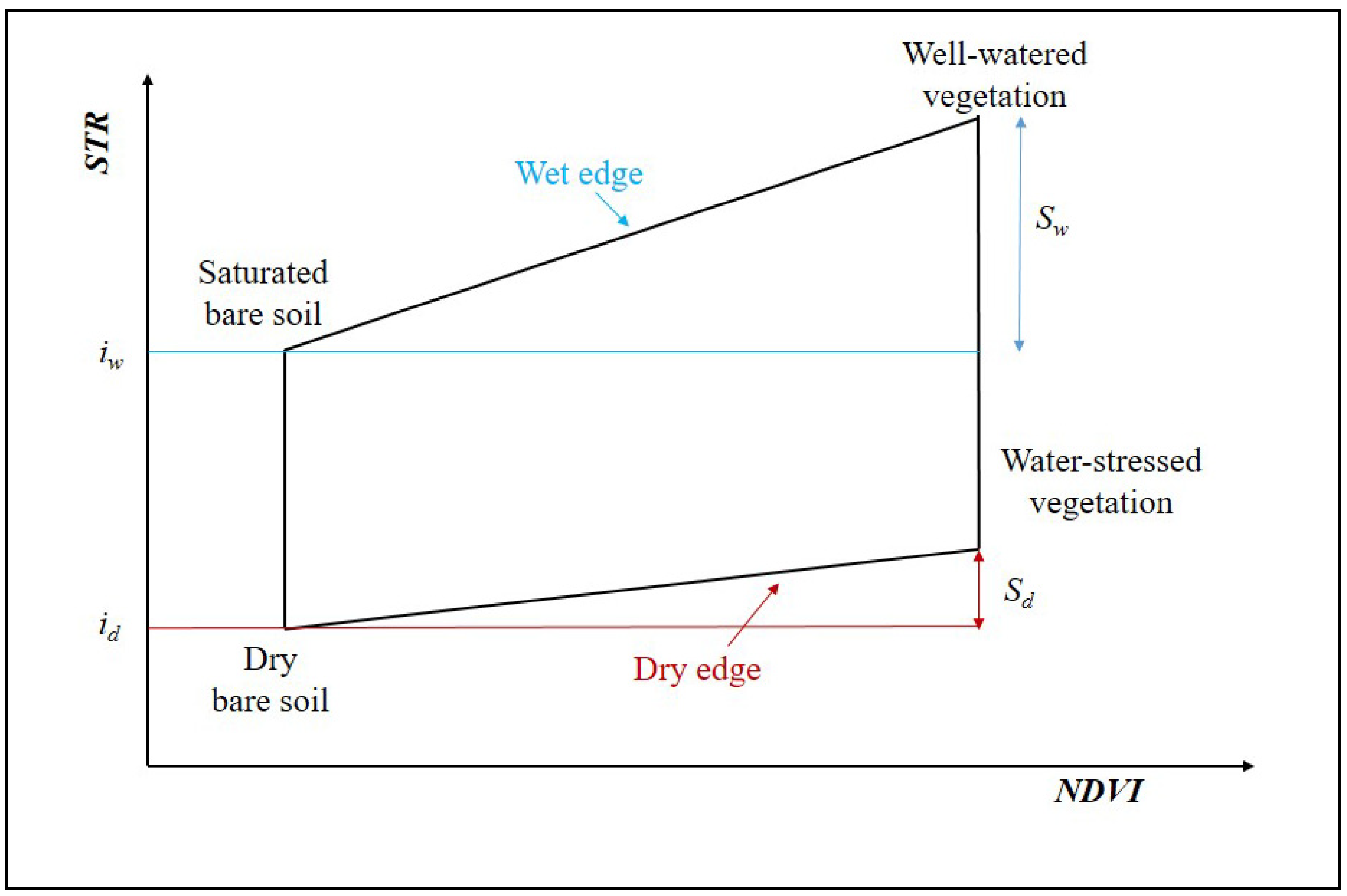
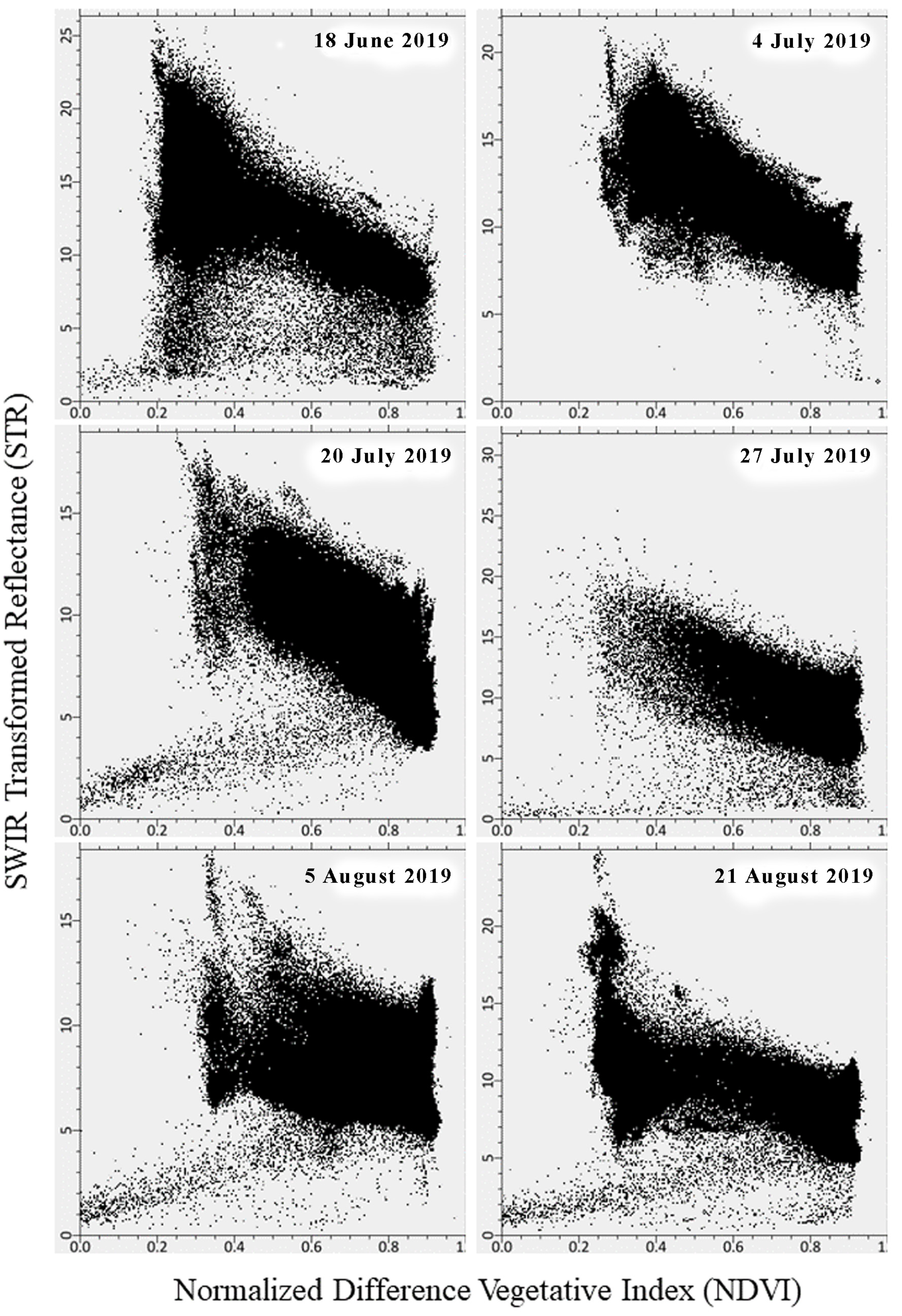
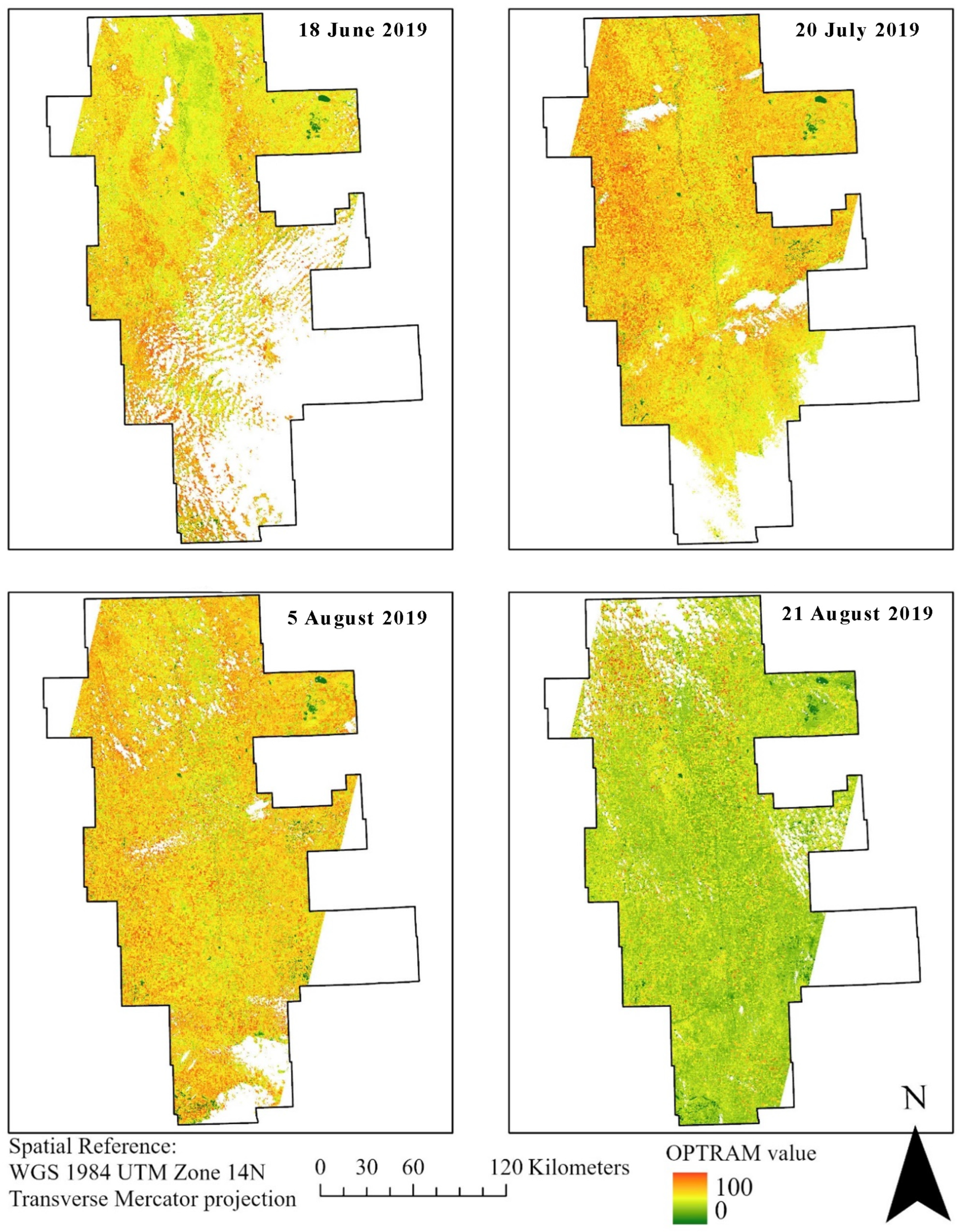
Multispectral NASA Landsat 8 (L8) satellite images were acquired from the United States Geological Survey (USGS) Earth Explorer (URL: https://earthexplorer.usgs.gov/, accessed on 1 December 2019) for the study area. Landsat 8 houses the Operational Land Imager (OLI) and the Thermal Infrared Sensor (TIRS), which image the land surface at 11 spectral bands in the optical and thermal infrared domains with 30 m to 100 m spatial resolution and 16-day temporal resolution. A total of 28 level-1 L8 images acquired in the 2019 growing season were used in this study (Table 1). The Fmask algorithm was used to detect and remove clouds and cloud shadows for all Landsat imagery [45].
Radiometric corrections of the multispectral bands were performed using the Fast Line-of-sight Atmospheric Analysis of Spectral Hypercube (FLAASH) toolbox, included in the Environment for Visualizing Image (ENVI) 5.5 software (https://www.harrisgeospatial.com/, accessed on 1 January 2020). The FLAASH atmospheric correction algorithm was chosen due to its better performance compared to algorithms, such as Quick Atmospheric Correction (QUAC) and Dark Object Subtraction (DOS) [46]. After removing clouds and obtaining the atmospheric corrected bands, a variety of moisture-related indices were calculated for each pixel, as described below.
Six moisture-related indices were calculated using band math toolbox of ENVI software. These indices included NDVI, NDWI, NDMI, EVI, SIPI, and ARVI. The moisture-related indices were calculated using equations that involve different bands (blue, green, red, NIR, SWIR) and ranges (descriptions shown in Table 2). Those images of the moisture-related index were processed in ArcGIS pro software and pixel values for each location of soil sampling were extracted from the image. These normalized values of moisture-related indices were then plotted against the measured in-situ surface SM (VWC).
Where, wavelengths range for blue band is 0.450–0.515 µm; green band is 0.525–0.600 µm; red (R) band is 0.600–0.680 µm; near infrared (NIR) band is 0.845–0.885 µm; and shortwave infrared (SWIR) band is 1.560–1.660 µm at Landsat 8 satellite image.

2.3.2. OPTRAM Model

The OPTRAM model developed by Sadeghi et al. [28] to estimate SM is a physically based trapezoidal space of pixel distribution within the STR-NDVI space (Figure 2). The NDVI is normalized difference vegetation index and STR is SWIR transformed reflectance [54]. The OPTRAM model only uses optical data, which means that no thermal infrared data area is used for retrieving SM. The normalized SM content (W) for each pixel was estimated from the dry edge and wet edge parameters, as follows:
W = (STR − STRd)/(STRw − STRd)
where, STR is the SWIR transformed reflectance, as follows:
STR = (1 − RSWIR)2/2RSWIR
where, STRd and STRw are STR at the dry (e.g., θd~0%, where θd is SM content) and wet (e.g., θs~100%, where θs is SM content) states, respectively, and RSWIR is surface reflectance for SWIR electromagnetic domain (1650 nm corresponding to band 6 of the Landsat 8).
The STR-NDVI space forms a trapezoid shape based on the assumption of a linear relationship between soil- and vegetation-water contents. Therefore, the parameters for Equation (3) can be obtained for a specific location in the satellite scene from the dry and wet edges of the optical trapezoid.
STRd = id + Sd NDVI
STRw = iw + Sw NDVI
where, id and Sd are the intercept and slope of the dry edge and iw and Sw are the intercept and slope of the wet edge.
Based on the Equations (1)–(4), SM within a given satellite image pixel can be estimated from its STR and NDVI values:
W = [id + SdNDVI-STR]/[id − iw +(Sd − Sw)NDVI],
where, the saturation degree W can be expressed as θ (m3 m−3) when multiplied with the soil porosity.
Google Earth Engine (GEE) was used to process Landsat 8 images for the study period and area to obtain SM maps via the OPTRAM model. GEE provides access to archived Landsat data, which includes Landsat 5, Landsat 7 and Landsat 8 OLI/TIRS from 2013 [55]. GEE was used to obtain STR, NDVI, and OPTRAM surface SM maps, as suggested by Yadav et al. [36] and Huang et al. [56].

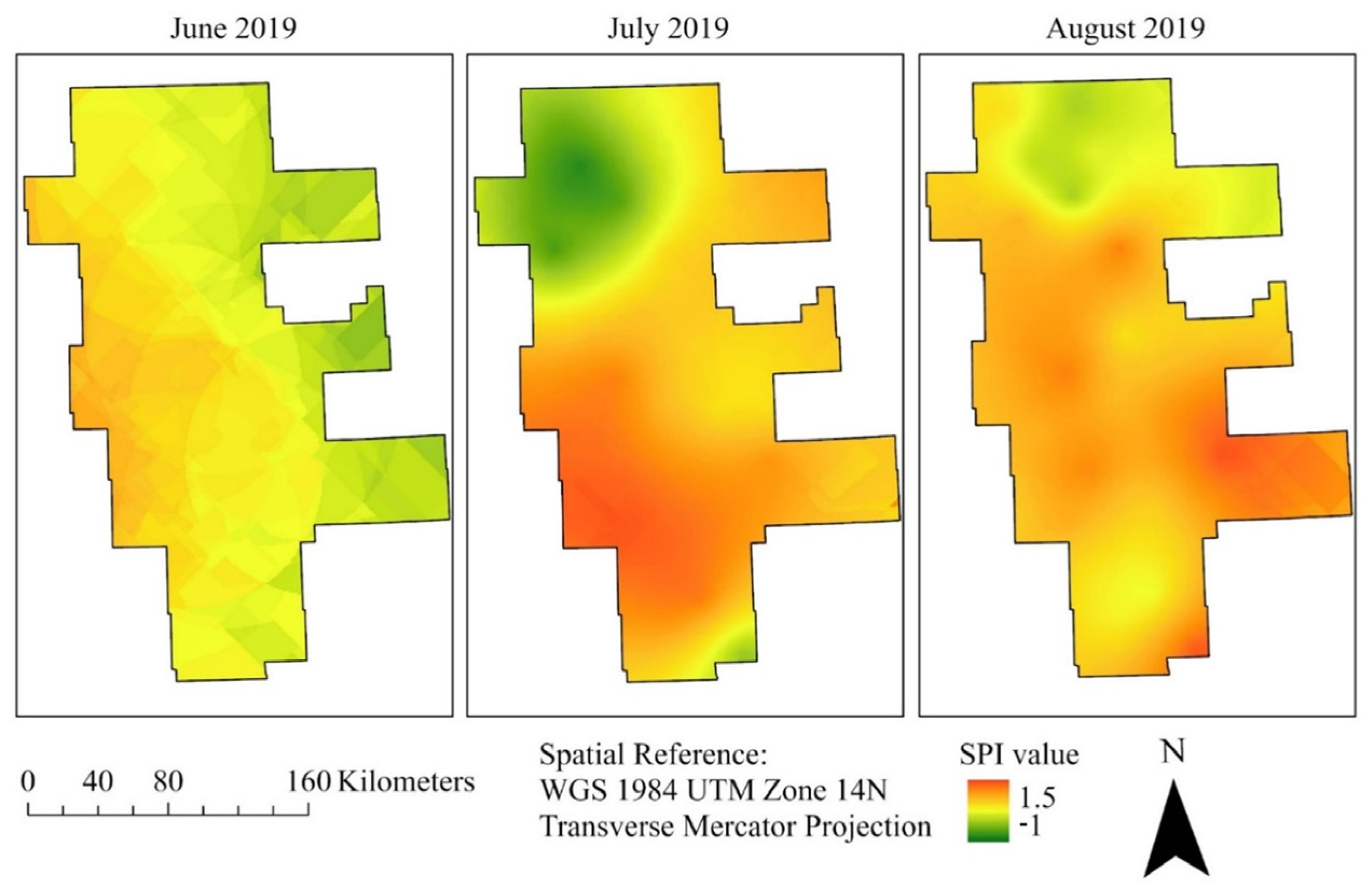
2.3.3. Standardized Precipitation Index (SPI)

The change in precipitation over time has direct impacts on groundwater, reservoir storage, surface SM, snowpacks, and stream flow. SPI is a statistical method developed by McKee et al. [57] for assessing rainfall. It is often preferred over the mean precipitation as a representation of the normal daily rainfall. For calculating SPI, the observed rainfall values from previous years are fitted to a gamma distribution and then transformed to a Gaussian distribution [58]. For this study, we used R statistical software 2020 using the precintcon R-package.
SPI was designed to quantify the precipitation deficit for multiple timescales, and reflects the impact of drought based on the rainfall in a specific year. In this study, we are establishing precipitation and surface SM that respond on a relatively short time scale. Precipitation data were collected from the weather stations since their establishment dates (1990–2005) and the SPI was calculated. The SPI values range from ±2, where +2 is extremely wet, −2 is extremely dry, and −1 to +1 is near normal conditions [59]. For this study, we calculated monthly SPI values that displayed the percentage of normal precipitation for 30-day periods.

2.4. Model Development and Workflow

The following paragraphs describe the model development and workflow for objectives 2, 3, and 4 in this study (Figure 3). For objective 1, the Landsat 8 images for the study area through the 2019 growing season were processed by using ENVI software to establish relationships between the various moisture-related indices described in Section 2.3.1 above with the corresponding in-situ surface SM. For objective 2, Google Earth Engine was used to prepare SM saturation maps via the OPTRAM model proposed by Sadeghi et al. [26] and used by Yadav et al. [36] and Huang et al. [56]. Surface moisture for each location pixel was extracted from the OPTRAM moisture map using ArcGIS Pro® to establish relationship with in-situ surface SM (Figure 3).
For objective 3, rainfall data from 25 weather stations for the entire 2019 growing season were downloaded from the NDAWN website (https://ndawn.ndsu.nodak.edu, accessed on 1 December 2020), and the four-day cumulative rainfall (mm) amounts for each soil sampling date (day of Landsat 8 satellite overhead pass) were calculated. Four-day cumulative rainfall maps were created using the rainfall values and ArcGIS Pro® ordinary kriging geospatial tool. SPI maps were also created using ordinary kriging for each month based on SPI values previously calculated in the R-software environment. The SPI maps were created for three months (June, July, and August) and cumulative rainfall maps were developed for four dates (18 June, 20 July, 5 August, and 21 August) for the 2019 growing season. Percent clay figures for each sampling location were extracted from the map downloaded from the University of California Davis—California soil resources lab. The pixel size of the maps was maintained at 30 m × 30 m.
The OPTRAM model’s SM, four-day cumulative rainfall, SPI and percent clay values were all extracted from the respective maps for each soil sampling location. The selection of these four variables is based on the study conducted by Acharya et al. [60] These four variables were used as predictor variables for in-situ surface SM in a random forest regression model (RFR), as described by Breiman [61]. The whole dataset was divided into training and testing data at a 70:30 ratio. The training dataset was used to develop the random forest regression algorithm and the testing dataset was used for validation. The validation was assessed by the model’s RMSE and coefficient of determination (r2). The selection of the RFR for prediction was based on the study conducted by Acharya et al. [60] comparing different machine learning models for predicting soil moisture in RRVN. See Acharya et al. [60] for a detailed description of the RFR algorithm.
The trained and validated random forest regression algorithm was then applied to selected agricultural fields within Cass County, North Dakota to estimate surface SM. The OPTRAM SM, percent clay, four-day cumulative rainfall, and SPI were extracted from each pixel (30 m × 30 m) in the selected area. The extracted values were then used as inputs for the trained random forest algorithm in the R-software environment to predict the area’s surface SM, and the output was mapped in ArcGIS Pro® using the pixel-by-pixel method.

3. Results

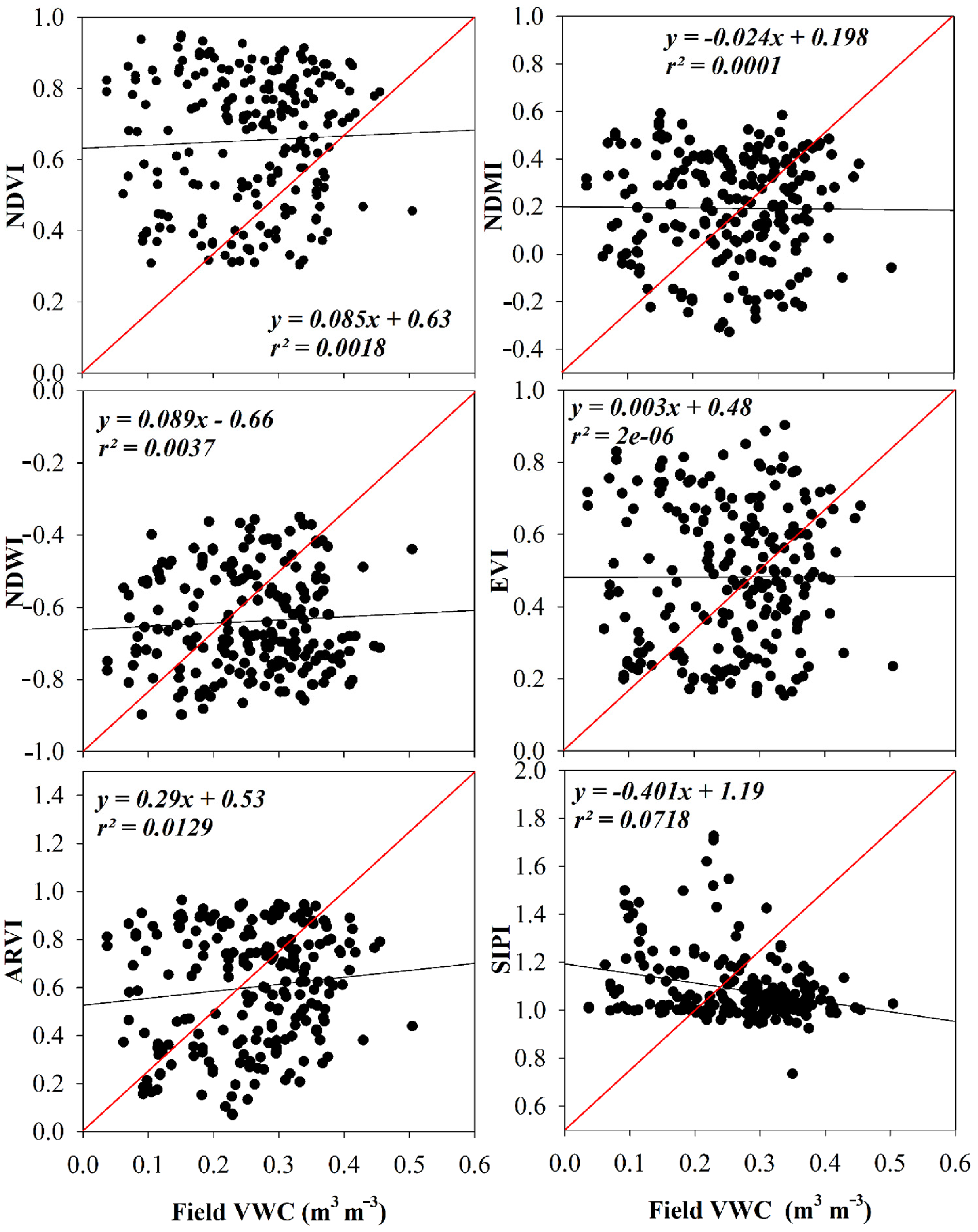
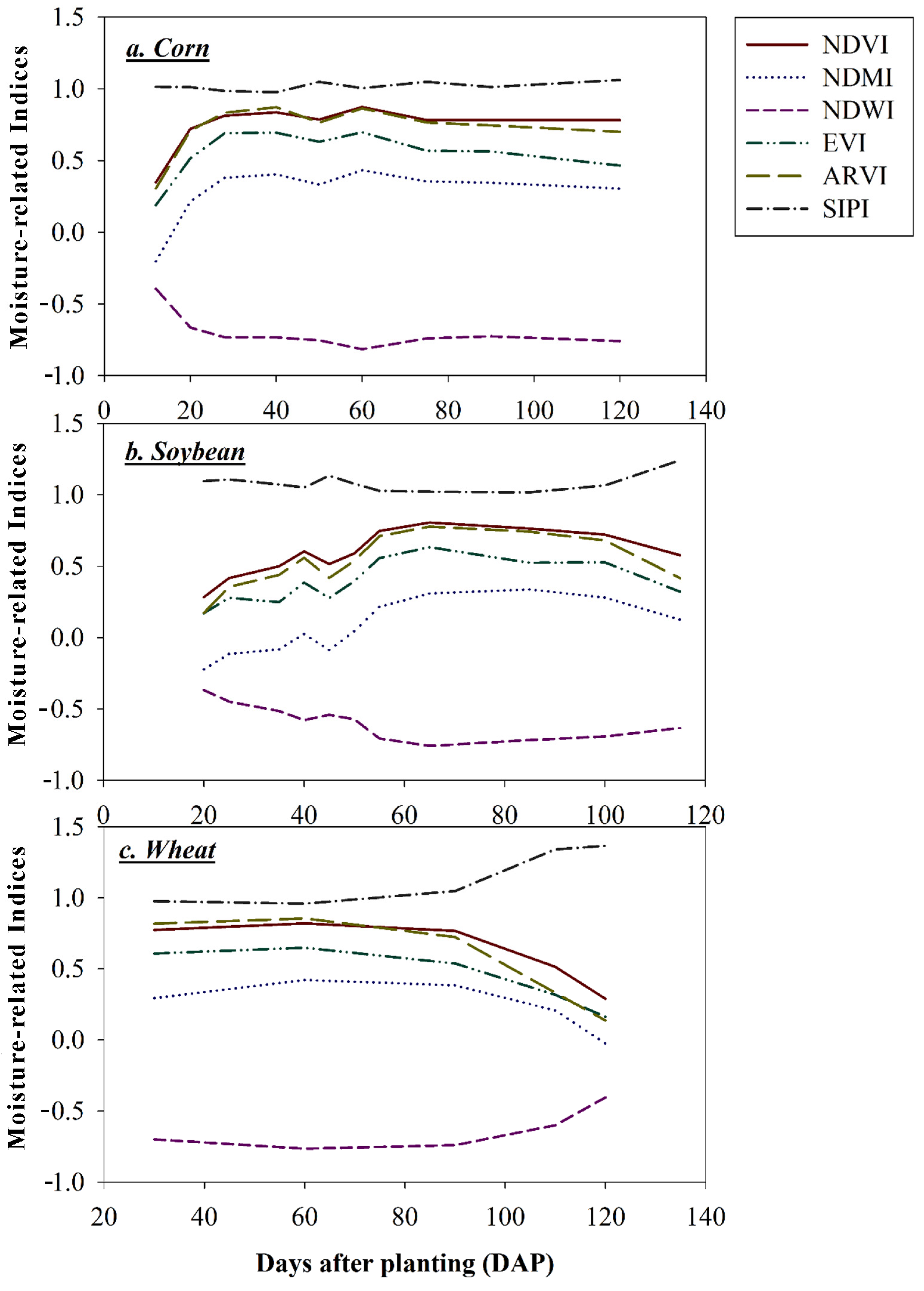
3.1. Relationship between Moisture-Related Indices and Surface SM

No relationship was observed between the moisture-related indices and the surface SM content for the entire study area and growing season (Figure 4). The scatter plot showed that none of the sample points lie around the bisector line (red colored line) for all the moisture-related indices, with r2 values less than 0.10 and slopes less than 0.20. The NDVI values for corn increased with vegetative growth after the emergence until the silking stage (Figure 5). Afterwards, the NDVI values remained the same until the crops started drying and were ready for harvest. The rate of increase is different for the soybean and wheat, but the NDVI values remain mostly constant after closure of the leaf canopies and crops grain fill. The NDVI values after planting remained the same for 80 days for all crops until drying and harvesting.
Early in the growing season, there was some bare ground on the corn and soybean fields, but the wheat field was quickly covered with greenness after emergence. This can be observed in the NDMI values (Figure 5), where early stages in the corn and soybean crops showed negative values; however, there were positive values in the wheat fields. In the NDMI values, variation was observed until the full canopy was observed in all crops, and not much change was observed afterwards. Unlike the NDVI and NDMI, the values are less for NDWI, and approaches −1 when the crop is at peak vegetative growth. A similar trend to NDVI was also observed with EVI and ARVI for all crops and days after planting. SIPI for all crops did not change much with growth stages because it is based on the leaf area index, chlorophyll, and carotenoid content. The values for each crop are different, but changes within the crop growth stages are minimal.

3.2. Surface SM Prediction Using OPTRAM

The pixel distribution within the STR-NDVI space for different days (18 June–21 August) did not show distinct trapezoidal shapes (Figure 6). Each of the six days exhibited a wide range of SRT and NDVI values due to the variability of SM and land cover. In general, STR and NDVI values are larger at the peak vegetative state (27 July 2019) compared to early and later crop growth stages.
SM maps created with the OPTRAM model showed the surface SM values were higher in the month of July and in early August compared to early June and later August (Figure 7). However, the performance of OPTRAM in predicting the surface SM was poor, as shown in terms of the regression slope, r2 and RMSE (Figure 8). The regression slopes for all dates are less than 0.20 with negative slope values on multiple dates.

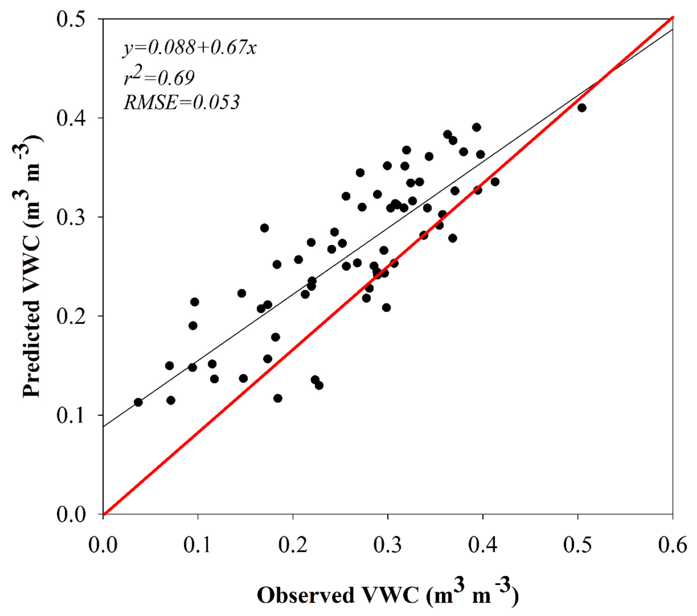
3.3. Surface SM Mapping with a Random Forest Algorithm

The RFR algorithm’s validation showed a high goodness of fit (r2 = 0.69) and low RMSE value (0.053 m3 m−3) (Figure 9) with just the four predictor variables (SPI, four-day cumulative rainfall, percent clay values, and the OPTRAM SM). The SPI for each month (June, July, and August) and four-day cumulative values for the specific dates of satellite passage (18 June, 20 July, 5 August, and 15 August) showed a wide range of values. The SPI values ranged from −0.26 to 0.94 for June, −0.78 to 1.40 for July, and −0.14 to 1.40 for August 2019 (Figure 10). This showed that July had normal precipitation over the study area, while the July and August months were wetter this year compared to previous years. Negative SPI values indicate less than median precipitation (dry conditions), and positive values indicate greater than median precipitation (wet conditions). However, four-day cumulative rainfall for 18 June was observed to be the lowest for the entire study area (5.38 to 21.55 mm) compared to 21 August, which ranged from 0 to 48.20 mm. For 20 July and 5 August, the cumulative rainfall was similar, ranging from 0 to 37.37 mm and 0.31 to 37.22 mm (Figure 11). Some parts of the study area had not received rainfall for the past four days, on two dates (July 20 and August 21).
Each pixel value of SPI, four-day cumulative rainfall, percent clay, and OPTRAM SM among the selected areas of the agricultural fields in Cass County, ND were used to demonstrate mapping of the algorithm’s surface SM (Figure 12). The surface SM for all four dates range from 0.22 to 0.39 m3 m−3. The surface SM values on 18 June and 21 August were less compared to 20 July and 3 August.

4. Discussion

4.1. Surface SM Estimation Using Moisture-Related Indices

The moisture-related indices used in this study are interrelated based on the Landsat 8 bands used to calculate them (Figure 13). This interrelation is likely part of the reason why all the moisture-related indices were similar in their poor performance regarding the indication of surface SM. The NIR band is common in the calculation of all moisture-related indices. In addition to the NIR band, the NDVI used the red band, NDWI used the green band, NDMI used the SWIR band, and SIPI used the blue band for calculation. EVI and ARVI are two indices that have used red and blue bands, along with NIR. Green vegetation strongly reflects NIR bands, and green vegetation is directly related to the moisture of the soil where it is grown. The red band of the spectrum is absorbed by the vegetation, the SWIR band discriminates the moisture content of the soil and vegetation. The blue band is sensitive to the chlorophyll and carotenoid molecules of the plant leaf, and the green band boosts water information. All the moisture-related indices are useful tools for measuring greenness based on the crop vegetative growth, but are not useful to indicating surface SM in the RRVN.
Cushion et al. [62] also found little to no relationship between NDVI and surface SM in the time series data. In contrast, Martyniak et al. [63] claimed that water availability in the root zone is one of the main factors controlling crop growth and vegetation status, hence, SM can be represented by the NDVI. Wang et al. [64] concluded mapping root-zone SM is challenging because the relationship between the NDVI and root-zone SM is dependent on the vegetation species and climate zones. They noted that NDVI derived from satellite images may provide a proxy for root-zone SM mapped at large scales. Adegoke and Carleton [65] found neutron probe measurements of SM taken in forest and crop sites are weakly correlated with full-resolution NDVI for each pixel. They also found the association measured by Pearson correlation coefficient between NDVI and SM is stronger over the forest than over the cropland during the growing season. NDVI, along with other moisture-related indices (NDMI, NDWI, EVI, ARVI, and SIPI), showed the same trend during the growing season for the three major crops in the RRNV of our study. The region of the RRVN in this study has a continental climate [66], thick underlying glaciolacustrine deposits of low permeability, and shallow perched water tables [67]. We observed that fields did not dry to levels where plants were water-stressed enough to affect crop physiology and vegetative growth. This may be due to adequate root-zone SM and shallow ground water tables serving as a supply of water, even when surface SM is quite low. This would likely result in the low variability in the values of moisture-related indices.

4.2. Effectiveness of OPTRAM to Predict Surface SM

The weak relationship between the OPTRAM model’s estimated SM and the actual field surface SM may have been partly due to high values of SRT coupled with low NDVI in the peak vegetative stage. This can occur when there is water in excess of saturated SM. The soils in the RRVN are derived from an ancient glaciolacustrine lakebed with high clay content and poor internal drainage, and are prone to flooding. Water in excess of the saturated SM will cause an increase in STR while the actual SM cannot increase beyond the saturated SM content [28,54].
Similar results were observed by Babaeian et al. [35] across the diverse climate of the United States, where r2 ranges from 0.01 to 0.49 and RMSE ranges from 5–8%. They used the OPTRAM model to estimate SM in Arizona, California, and Georgia, and found a nearly trapezoidal shape by STR-NDVI points. They observed that distributions of STR-NDVI points differ with the area under study due to the characteristics of climate and land cover. Yadav et al. [36] also used the OPTRAM model to predict SM in the Lalitpur district of India and found that the accuracy of this model was less than 10% when compared with other models (thermal). However, Yadav et al. [36] concluded that this reduced accuracy might be due to the lack of penetration of optical bands in the fully or densely covered vegetation. Similarly, Chen et al. [37] evaluated OPTRAM-based SM estimates using MODIS data, providing an overall RMSE from 0.05 to 0.13 m3 m−3, and r2 from 0.10 to 0.50, respectively, which corroborates our results. The poor performance shown by the OPTRAM SM estimates related to in situ SM might be due to the rough image resolution and heterogeneous terrains [37].

4.3. Machine Learning for SM Prediction

As anticipated, the RFR algorithm we developed substantially outperformed the other methods for predicting SM in the RRVN. Moreover, this was accomplished with very few input variables (n = 4) from typical weather stations and soil maps. Recently, machine learning algorithms for remote sensing data have been used elsewhere to predict SM with varying success [68,69,70,71,72]. Adab et al. [68] compared four different machine learning models (support vector machine (SVM), artificial neural network (ANN), elastic net regression, and RFR) for predicting near-surface SM in semi-arid Iran using Landsat 8 images, and found the highest explanatory ability (NS = 0.73) with the RFR algorithm. Similarly, Araya et al. [69] compared five machine learning models (ANN, SVM, support vector regression, relevance vector regression, and boosted regression trees) using an unmanned aircraft system (UAS) to capture reflectance (green, red, and near infrared) along with topographic and meteoric (rainfall and precipitation) variables to predict surface SM. They found that the RFR and BRT models performed better, with a rate of error less than 4% regarding volumetric soil water content. In other models, soil temperature has been replaced by the difference in temperature between LST and air temperature at 2 m above ground [73], this was addressed by SPI in our model.
Overall, the integration of machine learning (particularly RFR) with physically based remote-sensing models and commonly available weather and soil data appears to be a reliable tool for estimating and mapping surface SM at high resolutions across temperate, arid, and now frigid soil landscapes, deep and shallow water tables, and with a wide range of homogenous and heterogeneous vegetation. Future research efforts should be aimed at directly resolving the STR-NDVI space issues of the OPTRAM model in landscapes with frequent or prolonged flooding, discontinuous water-filled potholes, and permafrost, and/or aimed at indirectly resolving these issues by identifying key parameters to include in the machine learning algorithm input.

5. Conclusions

Remote sensing and machine learning are powerful tools that can not only cover a large area, but also process a large amount of data, and can be used in moisture prediction. This study showed the integrated use of satellite images, weather stations, and soil properties to predict the surface SM of agricultural fields. Six moisture-related indices calculated by using the ENVI platform showed poor relationships with infield SM. The weak relationships were established due to the differences in crop growth stages and canopy cover. In extreme drought conditions, moisture-related indices may reflect low SM content. OPTRAM SM maps developed by using Google Earth Engine also showed a weak relationship with infield surface moisture content. However, the SM prediction improved significantly after OPTRAM values were incorporated with rainfall, SPI, and percent clay using a random forest regression machine learning algorithm. SM prediction under environmental conditions might require the use of different linear and non-linear regression techniques. This needs to be tested in future. This research proposed an integrated model to predict surface SM over a larger area using easily available satellite images and weather stations. However, this model has to be tested in different areas and must consider other possible factors that can affect surface SM, depending on the landscape and location.

Author Contributions

Conceptualization, U.A. and A.L.M.D.; Methodology, U.A., A.L.M.D. and P.G.O.; Software, U.A.; Validation, U.A., A.L.M.D. and P.G.O.; Formal Analysis, U.A.; Investigation, U.A. and A.L.M.D.; Resources, A.L.M.D. and P.G.O.; Data Curation, U.A.; Writing—Original Draft Preparation, U.A.; Writing—Review and Editing, A.L.M.D. and P.G.O.; Visualization, U.A.; Supervision, A.L.M.D.; Project Administration, A.L.M.D.; Funding Acquisition, U.A. and A.L.M.D. All authors have read and agreed to the published version of the manuscript.

Funding

This research was funded by the North Dakota Agricultural Experiment Station, USDA-NRCS-CIG 69-3A75-17-282, and USDA-NIFA Hatch project 1005366. North Dakota Water Resources Research Institute provided support for graduate student stipend.

Data Availability Statement

Data is contained within the present article.

Acknowledgments

The authors thank Nathan Derby, Zachery Leinter, and Megan Ostrand for help in collecting soil samples from weather stations around the Red River Valley and Sudha GC Upadhaya for assistance in writing machine learning codes in R-language.

Conflicts of Interest

The authors declare no conflict of interest.

References

  1. Lillesand, T.M.; Kiefer, R.W.; Chipman, J.W. Remote Sensing and Image Interpretation; John Wiley & Sons: Hoboken, NJ, USA, 2008. [Google Scholar]
  2. Bastiaanssen, W.G.; Molden, D.J.; Makin, I.W. Remote sensing for irrigated agriculture: Examples from research and possible applications. Agric. Water Manag. 2000, 46, 137–155. [Google Scholar] [CrossRef]
  3. Penuelas, J.; Filella, I.; Biel, C.; Serrano, L.; Save, R. The reflectance at the 950–970 mm region as an indicator of plant water status. Int. J. Remote Sens. 1993, 14, 1887–1905. [Google Scholar] [CrossRef]
  4. Tucker, C.J. Remote sensing of leaf water content in the near infrared. Remote Sens. Environ. 1980, 10, 23–32. [Google Scholar] [CrossRef]
  5. Zeng, W.; Xu, C.; Huang, J.; Wu, J.; Tuller, M. Predicting near-surface SM content of saline soils from NIR reflectance spectra with a Modified Gaussian model. Soil Sci. Soc. Am. J. 2016, 80, 1496–1506. [Google Scholar] [CrossRef]
  6. Zhang, D.; Zhou, G. Estimation of SM from optical and thermal remote sensing: A review. Sensors 2016, 16, 1308. [Google Scholar] [CrossRef] [PubMed] [Green Version]
  7. Zhang, D.; Tang, R.; Zhao, W.; Tang, B.; Wu, H.; Shao, K.; Li, Z.L. Surface soil water content estimation from thermal remote sensing based on the temporal variation of land surface temperature. Remote Sens. 2014, 6, 3170–3187. [Google Scholar] [CrossRef] [Green Version]
  8. Das, K.; Paul, P.K. Present status of SM estimation by microwave remote sensing. Cogent Geosci. 2015, 1, 1084669. [Google Scholar] [CrossRef]
  9. Verstraeten, W.W.; Veroustraete, F.; Feyen, J. Assessment of evapotranspiration and SM content across different scales of observation. Sensors 2008, 8, 70–117. [Google Scholar] [CrossRef] [Green Version]
  10. Wang, L.; Qu, J.J. Satellite remote sensing applications for surface SM monitoring: A review. Front. Earth Sci.-Prc 2009, 3, 237–247. [Google Scholar] [CrossRef]
  11. Peng, J.; Loew, A.; Merlin, O.; Verhoest, N.E. A review of spatial downscaling of satellite remotely sensed SM. Rev. Geophys. 2017, 55, 341–366. [Google Scholar] [CrossRef]
  12. Francois, C. The potential of directional radiometric temperatures for monitoring soil and leaf temperature and SM status. Remote Sens. Environ. 2002, 80, 122–133. [Google Scholar] [CrossRef]
  13. Sobrino, J.A.; Raissouni, N. Toward remote sensing methods for land cover dynamics monitoring, application to Morocco. Int. J. Remote Sens. 2000, 20, 353–366. [Google Scholar] [CrossRef]
  14. Levit, D.G.; Simpson, J.R.; Huete, A.R. Estimates of surface soil water content using linear combinations of spectral wavebands. Theor. Appl. Climatol. 1990, 42, 245–252. [Google Scholar] [CrossRef]
  15. Dupigny-Giroux, L.A.; Lewis, J.E. A moisture index for surface characterization over a semiarid area. Photogramm. Eng. Rem. Sens. 1999, 65, 937–945. [Google Scholar]
  16. Sandholt, I.; Rasmussen, K.; Andersen, J. A simple interpretation of the surface temperature/vegetation index space for assessment of SM status. Remote Sens. Environ. 2002, 79, 213–224. [Google Scholar] [CrossRef]
  17. Tadesse, T.; Brown, J.; Hayes, M. A new approach for predicting drought-related vegetation stress: Integrating satellite, climate, and biophysical data over the U.S. central plains. ISPRS J. Photogramm. 2005, 59, 244–253. [Google Scholar] [CrossRef]
  18. Rouse, J.W.; Haas, R.H.; Schell, J.A.; Deering, D.W. Monitoring Vegetation Systems in the Great Plains with ERTS. Third Earth Resources Technology Satellite-1 Symposium; Technical Presentations, Section A; National Aeronautics and Space Administration (NASA SP-351): Washington, DC, USA, 1973; Volume I, pp. 309–317.
  19. Gao, B.C. NDWI—A normalized difference water index for remote sensing of vegetation liquid water from space. Remote Sens. Environ. 1996, 58, 257–266. [Google Scholar] [CrossRef]
  20. Ceccato, P.; Flasse, S.; Tarantola, S.; Jacquemond, S.; Gregoire, J. Detecting vegetation water content using reflectance in the optical domain. Remote Sens. Environ. 2001, 77, 22–33. [Google Scholar] [CrossRef]
  21. Jackson, T.J.; Chen, D.; Cosh, M.; Li, F.; Anderson, M.; Walthall, C.; Doriaswamy, P.; Hunt, E.R. Vegetation water content mapping using Landsat data derived normalized difference water index for corn and soybeans. Remote Sens. Environ. 2004, 92, 475–482. [Google Scholar] [CrossRef]
  22. Owe, M.; Chang, A.; Golus, R.E. Estimating surface soil moisture from satellite microwave measurements and a satellite derived vegetation index. Remote Sens. Environ. 1988, 24, 331–345. [Google Scholar] [CrossRef]
  23. Narasimhan, B.; Srinivasan, R.; Arnold, J.G.; Di Luzio, M. Estimation of long-term soil moisture using a distributed parameter hydrologic model and verification using remotely sensed data. Trans. ASAE 2005, 48, 1101–1113. [Google Scholar] [CrossRef]
  24. Liang, S.L. Quantitative Remote Sensing of land Surface; John Wiley & Sons: Hoboken, NJ, USA, 2004. [Google Scholar]
  25. Rahimzadeh-Bajgiran, P.; Berg, A.A.; Champagne, C.; Omasa, K. Estimation of SM using optical/thermal infrared remote sensing in the Canadian Prairies. ISPRS J. Photogramm. 2013, 83, 94–103. [Google Scholar] [CrossRef]
  26. Shafian, S.; Maas, S.J. Index of SM using raw Landsat image digital count data in Texas high plains. Remote Sens. 2015, 7, 2352–2372. [Google Scholar] [CrossRef] [Green Version]
  27. Sun, H. Two-stage trapezoid: A new interpretation of the land surface temperature and fractional vegetation coverage space. IEEE J. Sel. Topics Appl. Earth Observ. Remote Sens. 2016, 9, 336–346. [Google Scholar] [CrossRef]
  28. Sadeghi, M.; Babaeian, E.; Tuller, M.; Jones, S.B. The optical trapezoid model: A novel approach to remote sensing of SM applied to Sentinel-2 and Landsat-8 observations. Remote Sens. Environ. 2017, 198, 52–68. [Google Scholar] [CrossRef] [Green Version]
  29. Leng, P.; Song, X.; Duan, S.; Li, Z. A practical algorithm for estimating surface SM using combined optical and thermal infrared data. Int. J. Appl. Earth. Obs. 2016, 52, 338–348. [Google Scholar] [CrossRef]
  30. Pan, F.; Peters-Lidard, C.D.; Sale, M.J. An analytical method for predicting surface soil moisture from rainfall observations. Water Resour. Res. 2003, 39. [Google Scholar] [CrossRef] [Green Version]
  31. Gupta, M.; Srivastava, P.K.; Islam, T.; Ishak, A.M.B. Evaluation of TRMM rainfall for soil moisture prediction in a subtropical climate. Environ. Earth Sci. 2014, 71, 4421–4431. [Google Scholar] [CrossRef]
  32. Leng, P.; Li, Z.; Duan, S.; Gao, M.; Huo, H. A practical approach for deriving all-weather SM content using combined satellite and meteorological data. ISPRS J. Photogramm. 2017, 131, 40–45. [Google Scholar] [CrossRef]
  33. Brocca, L.; Moramarco, T.; Melone, F.; Wagner, W. A new method for rainfall estimation through SM observations. Geophys. Res. Lett. 2013, 40, 853–858. [Google Scholar] [CrossRef]
  34. Yu, W.; Ma, M.; Li, Z.; Tan, J.; Wu, A. New Scheme for validating remote-sensing land surface temperature products with station observations. Remote Sens. 2017, 9, 1210. [Google Scholar] [CrossRef] [Green Version]
  35. Babaeian, E.; Sadeghi, M.; Franz, T.E.; Jones, S.; Tuller, M. Mapping SM with the OPtical TRApezoid Model (OPTRAM) based on long-term MODIS observations. Remote Sens. Environ. 2018, 211, 425–440. [Google Scholar] [CrossRef]
  36. Yadav, S.K.; Singh, P.; Jadaun, S.P.S.; Kumar, N.; Upadhyay, R.K. SM analysis of Lalitpur district Uttar Pradesh India using Landsat and sentinel data. In Proceedings of the International Archives of the Photogrammetry, Remote Sensing & Spatial Information Sciences, ISPRS-GEOGLAM-ISRS Joint Int. Workshop on “Earth Observations for Agricultural Monitoring”, New Delhi, India, 18–20 February 2019; Volume XLII-3/W6. [Google Scholar]
  37. Chen, M.; Zhang, Y.; Yao, Y.; Lu, J.; Pu, X.; Hu, T.; Wang, P. Evaluation of the OPTRAM Model to retrieve soil moisture in the Sanjiang Plain of Northeast China. Earth Space Sci. 2020, 7, e2020EA001108. [Google Scholar] [CrossRef]
  38. Vicente-Serrano, S.M.; Pons-Fernández, X.; Cuadrat-Prats, J.M. Mapping SM in the central Ebro river valley (northeast Spain) with Landsat and NOAA satellite imagery: A comparison with meteorological data. Int. J. Remote Sens. 2004, 25, 4325–4350. [Google Scholar] [CrossRef]
  39. Alfieri, L.; Claps, P.; D’Odorico, P.; Laio, F.; Over, T.M. An analysis of the SM feedback on convective and stratiform precipitation. J. Hydrometeorol. 2008, 9, 280–291. [Google Scholar] [CrossRef] [Green Version]
  40. Hu, X.; Xue, M.; McPherson, R.A. The importance of soil-type contrast in modulating August precipitation distribution new the Edwards Plateau and Balcones Escarpment in Texas. J. Geophys. Res. Atmos. 2017, 122, 711–728. [Google Scholar] [CrossRef]
  41. Ali, I.; Greifeneder, F.; Stamenkovic, J.; Neumann, M.; Notarnicola, C. Review of machine learning approaches for biomass and SM retrievals from remote sensing data. Remote Sens. 2015, 7, 16398–16421. [Google Scholar] [CrossRef] [Green Version]
  42. Paloscia, S.; Pampaloni, P.; Pettinato, S.; Santi, E. A comparison of algorithms for retrieving SM from ENVISAT/ASAR images. IEEE Trans. Geosci. Remote. 2008, 46, 3274–3284. [Google Scholar] [CrossRef]
  43. Reynolds, S.G. The gravimetric method of SM determination Part I: A study of equipment, and methodological problems. J. Hydrol. 1970, 11, 258–273. [Google Scholar] [CrossRef]
  44. USDA. United States Department of Agriculture, International Production Assessment Division. Metadata for Crops at Different Growth Stage. 2020. Available online: https://ipad.fas.usda.gov/cropexplorer/description.aspx?legendid=312 (accessed on 5 August 2020).
  45. Zhu, Z.; Wang, S.; Woodcock, C.E. Improvement and expansion of the Fmask algorithm: Cloud, cloud shadow, and snow detection for Landsat 4–7, 8, and Sentinel 2 images. Remote Sens. Environ. 2015, 159, 269–277. [Google Scholar] [CrossRef]
  46. Shi, L.; Mao, Z.; Chen, P.; Gong, F.; Zhu, Q. Comparison and evaluation of atmospheric correction algorithms of QUAC, DOS, and FLAASH for HICO hyperspectral imagery. In Remote Sensing of the Ocean, Sea Ice, Coastal Waters, and Large Water Regions; International Society for Optics and Photonics: Bellingham, WA, USA, 2016. [Google Scholar]
  47. Tucker, C.J. Red and photographic infrared linear combinations for monitoring vegetation. Remote Sens. Environ. 1979, 8, 127–150. [Google Scholar] [CrossRef] [Green Version]
  48. Mcfeeters, S.K. The use of Normalized Difference Water Index (NDWI) in the delineation of open water features. Int. J. Remote Sens. 1996, 17, 1425–1432. [Google Scholar] [CrossRef]
  49. Xu, H. Modification of normalised difference water index (NDWI) to enhance open water features in remotely sensed imagery. Int. J. Remote Sens. 2006, 27, 3025–3033. [Google Scholar] [CrossRef]
  50. Sims, D.A.; Gamon, J.A. Estimation of vegetation water content and photosynthetic tissue area from spectral reflectance: A comparison of indices based on liquid water and chlorophyll absorption features. Remote Sens. Environ. 2003, 84, 526–537. [Google Scholar] [CrossRef]
  51. Liu, H.Q.; Huete, A. A feedback-based modification of the NDVI to minimize canopy background and atmospheric noise. IEEE Trans. Geosci. Remote. 1995, 33, 457–465. [Google Scholar] [CrossRef]
  52. Penuelas, J.; Baret, F.; Filella, I. Semi-empirical indices to assess carotenoids/chlorophyll a ratio from leaf spectral reflectance. Photosynthetica 1995, 31, 221–230. [Google Scholar]
  53. Kaufman, Y.J.; Tanre, D. Atmospherically resistant vegetation index (ARVI) for EOS-MODIS. IEEE Trans. Geosci. Remote 1992, 30, 261–270. [Google Scholar] [CrossRef]
  54. Sadeghi, A.M.; Jones, S.B.; Philpot, W.D. A linear physically-based model for remote sensing of SM using short wave infrared bands. Remote Sens. Environ. 2015, 164, 66–76. [Google Scholar] [CrossRef]
  55. Google Earth Engine. Google Earth Engine: A Planetary-Scale Platform for Earth Science Data & Analysis. 2012. Available online: https://earthengine.google.com (accessed on 1 June 2020).
  56. Huang, H.; Chen, Y.; Clinton, N.; Wang, J.; Wang, X.; Liu, C.; Gong, P.; Yang, J.; Bai, Y.; Zheng, Y.; et al. Mapping major land cover dynamics in Beijing using all Landsat images in Google Earth Engine. Remote Sens. Environ. 2017, 202, 166–176. [Google Scholar] [CrossRef]
  57. Mckee, T.B.N.; Doesken, J.; Kleist, J. The relationship of drought frequency and duration to time scales. In Proceedings of the Eighth Conference on Applied Climatology, Anaheim, CA, USA, 17–22 January 1993; American Meteorological Society: Anaheim, CA, USA, 1993; pp. 179–184. [Google Scholar]
  58. Abramowitz, M.; Stegun, I.A. Handbook of Mathematical Functions with Formulas, Graphs, and Mathematical Tables; US Government Printing Office: Washington, DC, USA, 1948; Volume 55.
  59. NDMC. National Drought Mitigation Center. Explanation of the US Drought Monitor. 2008. Available online: http://droughtmonitor.unl.edu/classify.htm (accessed on 15 July 2020).
  60. Acharya, U.; Daigh, A.L.; Oduor, P.G. Machine learning for predicting field soil moisture using soil, crop, and nearby weather station data in the Red River Valley of the North. Soil Syst. 2021, 5, 57. [Google Scholar] [CrossRef]
  61. Breiman, L. Random Forest. Mach. Learn. 2001, 45, 5–32. [Google Scholar] [CrossRef] [Green Version]
  62. Cashion, J.; Lakshmi, V.; Bosch, D.; Jackson, T.J. Microwave remote sensing of SM: Evaluation of the TRMM microwave imager (TMI) satellite for the Little River Watershed Tifton, Georgia. J. Hydrol. 2005, 307, 242–253. [Google Scholar] [CrossRef]
  63. Martyniak, L.; Dabrowska-Zielinska, K.; Szymczyk, R.; Gruszczynska, M. Validation of satellite-derived soil-vegetation indices for prognosis of spring cereals yield reduction under drought conditions–Case study from central-western Poland. Adv. Space Res. 2007, 39, 67–72. [Google Scholar] [CrossRef]
  64. Wang, X.; Xie, H.; Guan, H.; Zhou, X. Different responses of MODIS-derived NDVI to root-zone SM in semi-arid and humid regions. J. Hydrol. 2007, 340, 12–24. [Google Scholar] [CrossRef]
  65. Adegoke, J.O.; Carleton, A.M. Relations between SM and satellite vegetation indices in the US Corn Belt. J. Hydrometeorol. 2002, 3, 395–405. [Google Scholar] [CrossRef] [Green Version]
  66. Bell, G.D.; Halpert, M.S. Climate assessment for 1997. Bull. Am. Meteorol. Soc. 1998, 79, S1–S50. [Google Scholar] [CrossRef] [Green Version]
  67. Remenda, V.H.; Cherry, J.A.; Edwards, T.W.D. Isotopic composition of old ground water from Lake Agassiz: Implications for late Pleistocene climate. Science 1994, 266, 1975–1978. [Google Scholar] [CrossRef]
  68. Adab, H.; Morbidelli, R.; Saltalippi, C.; Moradian, M.; Ghalhari, G.A.F. Machine learning to estimate surface SM from remote sensing data. Water 2020, 12, 3223. [Google Scholar] [CrossRef]
  69. Araya, S.N.; Fryjoff-Hung, A.; Anderson, A.; Viers, J.H.; Ghezzehei, T.A. Advances in SM retrieval from multispectral remote sensing using unmanned aircraft systems and machine learning techniques. Hydrol. Earth Syst. Sc. 2021, 25, 2739–2758. [Google Scholar] [CrossRef]
  70. Li, Y.; Li, M.; Li, C.; Liu, Z. Forest aboveground biomass estimation using Landsat 8 and Sentinel-1A data with machine learning algorithms. Sci. Rep. 2020, 10, 9952. [Google Scholar] [CrossRef]
  71. Satalino, G.; Mattia, F.; Davidson, M.W.; Le Toan, T.; Pasquariello, G.; Borgeaud, M. On current limits of SM retrieval from ERS-SAR data. IEEE Trans. Geosci. Remote 2002, 40, 2438–2447. [Google Scholar] [CrossRef]
  72. Paloscia, S.; Pettinato, S.; Santi, E.; Notarnicola, C.; Pasolli, L.; Reppucci, A.J.R.S.O.E. SM mapping using Sentinel-1 images: Algorithm and preliminary validation. Remote Sens. Environ. 2013, 134, 234–248. [Google Scholar] [CrossRef]
  73. Przeździecki, K.; Zawadzki, J. Modification of the Land Surface Temperature–Vegetation Index Triangle Method for soil moisture condition estimation by using SYNOP reports. Ecol. Indic. 2020, 119, 106823. [Google Scholar] [CrossRef]
Figure 1. Location of NDAWN stations in counties of ND and MN around the RRVN.
Remotesensing 14 03801 g001
Figure 2. Sketch illustrating parameters of the optical trapezoidal model (OPTRAM) (Equation (5)). OPTRAM is parameterized based on the pixel distributions within the STR-NDVI space and was proposed by Sadeghi et al. [28]. Adapeted with permission from Ref. [28].
Remotesensing 14 03801 g002
Figure 3. Flow chart showing the Landsat 8 image processing and SM prediction model using Random forest regression (RFR) algorithm.
Remotesensing 14 03801 g003
Figure 4. Scatter plot showing observed field VWC (m3 m−3) versus moisture-related indices (NDVI, NDMI, NDWI, EVI, ARVI, SIPI) for 2019 growing season in the RRVN using Landsat 8 images along with regression coefficient (r2) and linear equation.
Remotesensing 14 03801 g004
Figure 5. Changes in the values of moisture-related indices (NDVI, NDMI, NDWI, EVI, ARVI, SIPI) with the days after planting for three crops (corn, soybean, and wheat) for the 2019 growing season in the RRVN.
Remotesensing 14 03801 g005
Figure 6. Pixel distributions within the SRT-NDVI space for all of the images for the 2019 growing season (18 June to 21 August) in the RRVN.
Remotesensing 14 03801 g006
Figure 7. Surface SM maps generated with OPTRAM using Landsat 8 images for different dates (18 June, 21 July, 5 August, 21 August) of the 2019 growing season in the RRVN. White pixels represent maxed pixels due to water bodies, shadows, clouds, and rural/urban areas.
Remotesensing 14 03801 g007
Figure 8. SM estimated by OPTRAM compared to field SM for different dates during the 2019 growing season in the RRVN.
Remotesensing 14 03801 g008
Figure 9. Scatter plot showing observed versus predicted volumetric water content (m3 m−3) during the testing phase along with regression coefficient (r2) and root mean square error (RMSE) for random forest regression model.
Remotesensing 14 03801 g009
Figure 10. Standardized Precipitation Index (SPI) maps created using rainfall data from 25 weather stations by ordinary kriging interpolation in the RRVN for the June, July, and August months of 2019.
Remotesensing 14 03801 g010
Figure 11. Four-days cumulative rainfall maps created using past four-days rainfall data from 25 weather stations by ordinary kriging interpolation in the RRVN for the 2019 growing season (18 June, 20 July, 5 August, and 21 August).
Remotesensing 14 03801 g011
Figure 12. Predicted surface SM (m3 m−3) for four days (18 June, 20 July, 5 August, and 21 August) over the selected agriculture field in Cass County within the study area.
Remotesensing 14 03801 g012
Figure 13. Relationship between the moisture-related indices on how they are calculated using different Landsat 8 image bands (red, green, blue, near infrared, short wave infrared) and their formulas.
Remotesensing 14 03801 g013
Table 1. List of the Landsat 8 image (path/row) acquired over the study area covering weather stations in 2019.
Path/RowWeather StationDate Sampled (2019)
29/28Campbell, Mooreton, Wahpeton, Fargo Sabin6/11, 6/27, 7/13, 7/29, 8/14, 8/30, 9/15
30/26Forest River, Inkster, Warren, Grafton, St. Thomas, Kennedy, Cavalier, Humboldt6/18, 7/4, 7/20, 8/5, 8/21, 9/6, 9/22
30/27Leonard, Sabin, Fargo, Ulen, Prosper, Galesburg, Perely, Hillsboro, Ada, Waukon, Mayville, Finley, Eldred, Grand Forks, Forest River, Inkster, Warren, 6/18, 7/4, 7/20, 8/5, 8/21, 9/6, 9/22
31/26Grafton, St. Thomas, Kennedy, Cavalier, Humboldt, Forest River, Inkster6/25, 7/11, 7/27, 8/12, 8/28, 9/13, 9/29
Table 2. List of moisture-related indices along with formula used to calculate, and their range for Landsat 8 satellite images used in this study.
IndexFormula for CalculationRangeReference
Normalized Difference Vegetation Index (NDVI)NDVI = (NIR − R)/(NIR + R)−1 to +1; Where +1 represents dense green leaves and −1 represents a likely water body [47]
Normalized Difference Water Index (NDWI)NDWI = (Green − NIR)/(Green + NIR)−1 to +1; Where +1 represents extensive deep-water bodies and −1 represents vegetation cover[48,49,50]
Normalized Difference Moisture Index (NDMI)NDMI = (NIR − SWIR)/(NIR + SWIR)−1 to +1; Where +1 represents high canopy cover and no water stress and −1 represents low canopy cover to bare soil[19]
Enhanced Vegetation Index (EVI)EVI = 2.5[(NIR − R)/(NIR + 6R − 7.5Blue + 1)]−1 to +1; healthy vegetation generally falls between values of 0.20 to 0.80[51]
Structure Insensitive Pigment Index (SIPI)SIPI = (NIR − Blue)/(NIR − R)0 to 2; healthy green vegetation is from 0.8 to 1.8.[52]
Atmospherically Resistant Vegetation Index (ARVI)ARVI = (NIR − 2R + Blue)/(NIR + 2R + Blue)−1 to +1 healthy vegetation generally falls between values of 0.20 to 0.80[53]
Publisher’s Note: MDPI stays neutral with regard to jurisdictional claims in published maps and institutional affiliations.

