CAPS: A New Method for the Identification of Different Surface Displacements in Landslide and Subsidence Environments through Correlation Analysis on Persistent Scatterers Time-Series from PSI

Abstract

Persistent Scatterer Interferometry (PSI) is one of the most powerful tools for identifying and monitoring areas exposed to surface deformations such as landslides or subsidence. In this work, we propose a new method that we named CAPS (Correlation Analysis on Persistent Scatterers), to extend the capability of PSI in recognizing and characterising areas influenced by complex ground deformations and differential motions. CAPS must be applied to both ascending and descending orbits separately and comprises three major steps: (i) calculating the cross-correlation matrix on detrended PS time-series; (ii) extracting PS pairs with similarity greater than a given threshold; (iii) grouping PS in families by sorting and classification. Thus, in both orbits, PS Families identify groups of PS with similar movements. This allows distinguishing sectors characterised by different displacements over time even in areas with similar LOS (Line of Sight) velocities. As test sites, we considered four different known geological scenarios: two representing landslide environments (Santo Stefano d’Aveto and Arzeno, both in Liguria, NW Italy) and two subsidence environments (Rome and Venice, urban and surrounding areas). This method proved to be versatile, applicable to different geological situations and at different scales of observation, for recognizing both regional and local differential deformations.

1. Introduction

Ground movements, such as land subsidence and slope instabilities, represent a major threat to population, buildings and infrastructures, especially in a period of increasing frequency of drastic meteo-hydrologic phenomena [1,2,3]. Conducting a careful prevention campaign to identify and monitor risk areas is not always easy and is often very expensive with common in situ methods. In the last decades, the Interferometric Analysis of Synthetic Aperture Radar images (InSAR) has been proven to be a very important complementary tool to detect, quantify, and monitor landslides and urban subsidence, as well as deformation of volcanic edifices or seismogenic displacements [4,5,6,7]. The launch of the Sentinel-1A (2014) and Sentinel-1B (2016) satellites within the frame of the European Copernicus Programme [8] improved the capability of InSAR analysis, also thanks to the small repeat cycle of the satellites, which is 12 days each or 6 days considering both together, due to 180° shifting of their orbits.

Three InSAR techniques have been developed so far:

-

Differential Interferometry (DInSAR): ground deformation is analysed by comparing two successive SAR acquisitions;

-

Small Baseline Subset (SBAS): provides time-series of movements and velocity maps by long-term, multi-temporal analysis of pairs of SAR acquisitions with small spatial and temporal baselines;

-

Persistent Scatterer Interferometry (PSI): provides time-series of movements over natural or anthropogenic-based targets (e.g., outcrops, building, pylons), called Persistent Scatterers (PS), and/or over homogenous areas (e.g., non-cultivated lands, desert areas), called Distributed Scatterers (DS), by analysing at least 30–35 SAR acquisitions.

In this study, we developed a new method to improve the capability of PSI. PSI results are generally displayed in terms of time-series of displacement observed along the Line of Sight (LOS) of the satellite in both Ascending and Descending orbits. The angular coefficient of the line interpolating all the points of the time-series represents the mean LOS velocity (mm/y) of the PS. However, similar LOS velocities can derive from trends that could even be very different from each other. An example is reported in Figure 1 where two groups of PS with different time-series and similar LOS velocities (~0 mm/y) are shown. They likely refer to two different geologic situations that cannot be distinguished by exclusively considering their velocities. With our method, which we named CAPS (Correlation Analysis on Persistent Scatterers), we aim at a better characterisation of complex geological scenarios through an automatic identification of groups of PS (i.e., PS Families) with similar deformation trends without considering their velocity values. 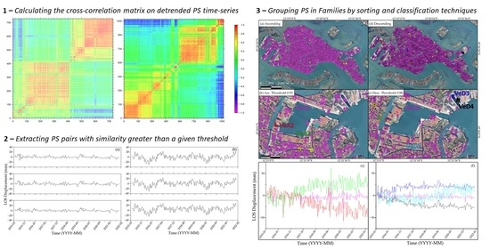CAPS is based on the Waveform Similarity Analysis (WSA), a method commonly used in seismology to find similar seismic events through the calculation of a cross-correlation matrix [9,10,11,12,13,14]. After extrapolating PS for both orbits, in the R software environment we detrended and removed the offset from the time-series. Then, we calculated the cross-correlation matrix from which we selected PS pairs with similarity greater than a chosen threshold. Finally, we recognised the PS Families by a sorting and classification technique.

We applied CAPS to both orbits to four different areas: Santo Stefano d’Aveto and Arzeno landslides, and Rome and Venice, where urban and surrounding areas are subject to differential subsidence motions. Furthermore, for Rome and Venice we cut a series of subscenes, thus also applying CAPS at different scales.

Results indicate that the PS Families found with CAPS are composed of neighbour PS characterised by time-series that are similar in shape. This allowed recognition of sectors with homogeneous deformation in both landslides and subsidence environments, from larger areas to localised sectors, down to single districts or groups of edifices. The application of CAPS proved to be a powerful and versatile tool, useful to better understand the kinematics of larger as well as more localised areas where several different movements can occur together.

The method presented in this paper is an improvement of the procedure used by [15] to investigate the landslide affecting Santo Stefano d’Aveto. In [15], PS Families were identified through a visual interpretation of the cross-correlation matrix. Specifically, the cross-correlation matrix was drawn using a suitable colour scale in order to visually identify PS Families. CAPS makes the analysis of the cross-correlation results more rigorous, faster and easier to apply to both orbits and to any case study. The families are defined through a multi-step algorithm (see Section 3.2) that automatically extracts groups of PS from the cross-correlation matrix, that have time series with a similarity greater than a given threshold. The results obtained by applying CAPS to the Santo Stefano d’Aveto landslide confirm what was already found by [15]; considering the descending orbit only, three sectors in the landslide characterised by different movements are clearly recognizable, in accordance with previous interpretations of in situ data [16,17].

2. Test Sites

In this work, we selected four different geological scenarios already analysed in previous studies (citations are in the next sub-paragraphs): two represent active landslide processes (Santo Stefano d’Aveto and Arzeno villages, both in Liguria, NW Italy) and two are active subsidence environments (Rome and Venice, urban and surrounding areas). Our scope is to present and test the CAPS method; thus, we will not discuss in depth the geological implication of our results and we just report a brief setting for each test site.

2.1. Santo Stefano d’Aveto

The village of Santo Stefano d’Aveto is located in the Ligurian Apennine, near the border between Liguria and Emilia-Romagna (NW Italy). The town centre is found in a lateral branch of the Aveto Valley, at about 1000 m a.s.l.; nearby, up to 1300 m a.s.l., there are some smaller hamlets, the most important being Roncolongo and Rocca d’Aveto. The valley of Santo Stefano is ENE–WSW oriented, and it is surrounded by some of the highest peaks of the Ligurian Apennine, reaching 1700–1800 m a.s.l.

The geology of the area is complex, with marly limestone flysch and sedimentary melanges comprising sandstones, heterogeneous breccias, and ophiolitic olistoliths (basalts, serpentinites) up to km in size [18,19]. The bedrock is covered by colluvial and landslide deposits.

The main geomorphological feature is a complex earth slide/earth flow landslide which extends along the valley floor [20] (Figure 2). According to the Italian Inventory of Landslide Phenomena (IFFI) [21], the landslide is divided into an active upper sector and a dormant lower sector. Recent studies involving different monitoring methodologies, both in situ and by remote sensing, show that both sectors are active; the upper sector is moving at about 40–50 mm/y, while the estimated speed of the lower sector is 20–30 mm/y [15,21,22,23].

2.2. Arzeno

Arzeno is a small village of the municipality of Ne (Liguria, NW Italy), located in the upper Graveglia valley, in the central-eastern Ligurian Apennine. The main town stands halfway up the eastern slope of the Graveglia valley, at about 600 m a.s.l. The slope goes from about 400 m a.s.l. on the valley floor to 1127 m a.s.l. by the top of Mt. Chiappozzo.

Bedrock formations outcropping in the Arzeno area belong to the Bracco-Val Graveglia Unit. They are composed of a Jurassic ophiolitic sequence (serpentinites, gabbros, basalts and associated ophiolitic breccias) overlayed by a Jurassic-Cretaceous deep-sea sedimentary sequence comprising cherts, limestones, and shales [25,26].

From the geomorphological point of view, evidence suggests the presence of a deep-seated gravitational slope deformation (DSGSD) that involves the entire slope from the Mt. Chiappozzo ridge to the valley floor [27]. This area is also affected by several complex landslides, among which the most relevant and well-known are the Arzeno landslide and the adjacent Prato landslide. The Arzeno landslide extends from about 850 m a.s.l. to the valley floor, where it causes a deviation of the Reppia stream. IFFI [21] identifies several sectors with different activity (Figure 3): active sectors have been identified by the Arzeno settlement and in the lower part of the landslide, near the valley floor; other sectors of the landslide are classified as dormant or stabilised. The Prato landslide extends from about 800 m a.s.l. to 450 m a.s.l., almost reaching the valley floor. The IFFI classifies it as a stabilised landslide.

Recent technical and scientific reports, by using several remote sensing and in situ monitoring methodologies, have estimated average speed of about 20 mm/y for the active sectors of both Arzeno and Prato landslides, with peaks of about 30–40 mm/y in correspondence of the Arzeno settlement [28,29].

2.3. Venice

Venice is the regional capital of Veneto, in north-eastern Italy. One of the most famous cities in the world, it is built on several small, sandy islands in the central part of the Venice Lagoon, near the coast of the Adriatic Sea. The city and the surrounding areas rest on Quaternary alluvial and tidal deposits (Figure 4). The thickness of the Quaternary deposits exceeds 700 m [30].

As it is located at sea level, the city of Venice is susceptible to sea level rise, which increases the risk of flooding due to tides and adverse meteorological conditions. Relative sea level rise has been calculated to be 0.23 m in the XX century; 0.11 m can be attributed to true sea level rise caused by climate change, while the rest is due to subsidence, caused by natural and anthropogenic causes such as the groundwater pumping in past decades and construction of new buildings [31].

As a consequence, subsidence in the area of Venice and the Venice Lagoon has been extensively studied [32,33]. Vertical displacement in the city averages is of the order of 0.8–1 mm/y; the ancient, pre-1500 part of the city is stabler compared to the more recent outskirts. Parts of the city, interested by reconstructions, restorations of buildings and other urban maintenance processes, show higher displacement rates that can be up to 10 mm/y for short time intervals [33]. Different sectors of the Venice Lagoon subside at different rates: the northern lagoon has a 2–3 mm/y rate of vertical displacement, while the southern lagoon has a 3–4 mm/y rate [32].

2.4. Rome

Rome, the Italian capital, is a city with 2.8 million inhabitants, located in the Lazio region in central Italy. The city stands on the lower part of the valley of the Tiber river, which flows across the urban area from NNE to SSW. In the northern part of the city, the Aniene river, coming from the E, flows into the Tiber. On the two sides of the main river, the landscape is characterised by low hills, which represent the lower foothills of the Colli Albani on the SE, the Sabatini Mountains on the NW and the Central Apennines on the NE. Southwest of the city lies the Tiber alluvial plain, which extends to the coast of the Tyrrhenian Sea.

The geology of the area is characterised by volcanic deposits belonging to the Sabatino volcanic district and the Albano volcanic district, Pleistocene marine deposits, and Meso-Cenozoic limestones outcropping on the Apennine foothills on the NE (Figure 5). The Tiber valley and the narrower Aniene valley are filled with alluvial deposits [35].

Ground subsidence in the city of Rome is well known and many studies have dealt with its quantification using InSAR techniques [4,36]. In most cases, subsidence is caused by the weight of construction on unconsolidated sediments. Thus, it is more evident on the alluvial material of the Tiber valley [37,38]. There are some cases, such as the Acque Albule plain, where groundwater extraction has played a major role [39].

Vertical motion due to subsidence in the urban area has been estimated between 2 to 5 mm/y, with peaks of 7–9 mm/y; the higher values are found along the Tiber valley. Even higher values, up to 20 mm/y have been observed for the area of the Fiumicino Airport, which is located in the Tiber alluvial plain near the Tyrrhenian coast. The nearby Lido di Ostia coastal zone shows vertical motion up to 12 mm/y [4].

3. Materials and Methods

3.1. PS Processing: Software and Data

We used Copernicus Sentinel-1A acquisitions from 2015 to 2022 for each test site, downloading 180-to-200 images for each orbit via the Alaska Satellite Facility (ASF) web repository (

Table 1. Information about the Sentinel-1A acquisitions used for each test site.

	Track	Frame	First Image	Last Image	Images	Master	Sub-Swath
Santo Stefano d’Aveto
Ascending	15	139, 141-2-3-4-5	23 March 2015	2 February 2022	205	17 August 2019	IW2
Descending	168	441-2-3-4-5-6-7	22 March 2015	1 February 2022	203	25 March 2019	IW3
Arzeno
Ascending	15	139, 141-2-3-4-5	18 November 2015	2 February 2022	184	7 April 2019	IW2
Descending	66	441-2-3-4-5-6	10 November 2015	6 February 2022	189	17 January 2019	IW1
Venice
Ascending	117	142-3, 145-6-7	30 March 2015	9 February 2022	204	28 October 2018	IW3
Descending	95	438-9, 440, 442-3	29 March 2015	8 February 2022	197	21 September 2018	IW2
Rome
Ascending	117	130-1, 133, 135-6	30 March 2015	9 February 2022	204	28 October 2018	IW2
Descending	22	450-1-2-3-4-5-6-7	24 March 2015	22 January 2022	192	21 April 2018	IW3

). They are Single Look Complex (SLC) TOPSAR data acquired in Interferometric Wide (IW) mode with VV Polarisation. The use of only Sentinel-1A acquisitions proved to be adequate for the purpose of this work; adding the Sentinel-1B dataset would have employed an excessive amount of computing time and storage space without giving appreciable improvements on the final results.

We conducted the PS processing using the latest available versions of the following open-source software:

(1)

SNAP (SeNtinel Application Platform) [41] that allows (i) selecting the Master image, (ii) correcting and splitting both Master and Slave images, (iii) co-registering each Slave with the Master and creating the relative interferograms, and finally (iv) exporting the resulting products in StaMPS format;

(2)

snap2stamps [42] that allows performing the previous ii to iv steps automatically for the entire stack of images with a series of python scripts;

(3)

StaMPS (Stanford Method for Persistent Scatterers) [43] that processes with multiple steps the products resulting from SNAP/snap2stamps to extrapolate PS velocity maps.

A detailed description of the processing chain and the StaMPS parameterization can be found in [4,42,43]. It is important to highlight that the StaMPS parameters greatly influence the final results, also depending on the analysed geological scenario; thus, a proper StaMPS setting is of utmost importance. The parameterizations used in this work for the landslide and subsidence test sites are shown in

Table 2. List of StaMPS parameters used in this research. The Default and the Used values together with the involved StaMPS steps are shown. Note that max_topo_error has been changed only for the two subsidence test sites.

Parameters	StaMPS Step	Default	Used	Environment
max_topo_error	2	20 m	10 m	Subsidence
unwrap_time_win	6	730 days	24 days	Both
unwrap_grid_size	6	200 m	10 m	Both
unwrap_gold_n_win	6	32	8	Both
scla_deramp	7	n	y	Both
scn_time_win	8	365 days	50 days	Both

. The choice has been made according to previous studies [15,44,45] on similar geological scenarios and by autonomously trying different settings. Below, the parameters we changed are described according to [43]:

-

max_topo_error: value in metre of the maximum uncorrelated DEM error accepted. Changed only for the subsidence cases;

-

unwrap_time_win: length in days of the time window used to filter/smooth the phase in time by estimating the noise for each pair of neighbouring pixels. Changed for both landslide and subsidence cases;

-

unwrap_grid_size: spacing of the resampling grid. Changed for both landslide and subsidence cases;

-

unwrap_gold_n_win: size of the window for the Goldstein filter [46]. Changed for both landslide and subsidence cases;

-

scla_deramp: it estimates the phase ramp for each interferogram (if set to “y”). Changed for both landslide and subsidence cases;

-

scn_time_win: window size of the low-pass temporal filter. Changed for both landslide and subsidence cases.

3.2. Waveform Similarity Analysis (WSA) and Correlation Analysis on Persistent Scatterers (CAPS)

In seismology, in order to better understand the seismic features of an area, it is useful to identify seismic events that present some degree of correlation. In particular, a group of earthquakes occurring very close in space and having a similar source-time function, propagation path, station site and recording instrument are defined as a “Family”. One of the most-used methods to identify earthquake families is the so-called Waveform Similarity Analysis, or WSA [12,47], which is based on seismogram cross-correlation.

Such a method can obviously be applied to other research fields whenever time-series need to be analysed. In this paper, we propose the application of the WSA for the identification of groups of PS showing similar time-series of ground movement and, therefore, to define areas characterised by similar deformation patterns at the surface.

In particular, the similarity between two PS time-series, a₁(t) and a₂(t), is estimated through the normalised cross-correlation function (NCCF) defined as (1):

$$NCCF \left(\tau \right)=\frac{C_{12}\left(\tau \right)}{\sqrt{C_{11}\left(0\right)C_{22}\left(0\right)}}$$

(1)

where τ is the time shift, and $C_{12}\left(\tau \right)$ is defined by (2):

$$C_{12}\left(\tau \right)={{\displaystyle \int }}_{-\infty }^{+\infty }{a}_1\left(t\right)a_2\left(t+\tau \right)dt$$

(2)

The maximum value assumed by NCCF (i.e., the cross-correlation coefficient) is indicative of the similarity between the signals. Therefore, the more two PS, a₁(t) and a₂(t), show similar time-series, the more the function NCCF will approach 1; 1 is the value assumed by the cross-correlation coefficient when signals are clones, −1 when signals are uncorrelated and 0 when signals are completely different.

After calculation of the cross-correlation coefficient for each pair of PS in a set, it is possible to define a cross-correlation matrix that can be visual inspected to define groups of PS having a similarity greater than a predefined threshold (Figure 6).

In order to identify PS Families within the cross-correlation matrix in a more objective way, we have developed a two-step algorithm. First, all pairs of PS showing a similarity greater than a certain threshold are identified and extracted from the matrix, then they are grouped in families through a sorting and classifying technique.

In the first step, the most important parameter that must be defined is the cross-correlation threshold, or index of similarity. The choice of the threshold value is crucial and is essentially based on subjective expert judgement. In many seismological applications [11,13,14], several decreasing values of the threshold are iteratively applied until the best compromise between the number of families and the population of each family is achieved. In this work we tuned such threshold following the previous rule and also considering the characteristics of the investigated PS dataset and the target of the analysis. Specifically, when dealing with small areas and a limited number of PS (e.g., <2000) and the goal is to identify significant heterogeneities in small-scale ground displacements, the threshold should be chosen considering low values (e.g., <0.90). Figure 7a shows an example of time-series of three PS with similarity greater than 0.83. If the analysis is performed on extended areas with a large number of PS (e.g., >10,000) and the goal is to identify slightly different deformations at larger scale, the threshold should be increased to values higher than the previous case (e.g., >0.90). Figure 7b shows an example of PS time-series with similarity greater than 0.95. In other words, the choice of the cross-correlation threshold can be used to guide the analysis towards different levels of resolution. In the next paragraph, we show some examples to explain the influence of the threshold value on the results.

In the second step, the algorithm used for defining the families is based on the Equivalence Class approach [48], already tested and applied to earthquake data sets by many authors [11,49,50].

Given the list of PS pairs with a level of similarity greater than the threshold, it is necessary to group elements that are in the same equivalence class of “sameness”. The adopted algorithm works like a “bridging technique”; if two pairs of PS (A, B) and (B, C) share a common PS (B) then all three PS are attributed to the same family even if the similarity between A and C is lower than the selected threshold value. Event B therefore represents the “bridge” between these pairs.

In summary, the proposed CAPS method is based on the following operative steps:

• Removal of the offset (offset removal) and of the linear trend (detrending) from the PS time-series using the “detrend” function of the package “pracma” of R;
• Calculation of the cross-correlation matrix through the “cor” function of the package “stats” of R;
• Selection of the PS pairs with a level of similarity greater than a certain cross-correlation threshold;
• Definition of PS Families through the “eclass” subroutine in Fortran 77 [48].

The outcomes resulting from the WSA are strongly dependent on the number of data points considered, which in our application corresponds to the number of SAR images processed. In general, for such analyses the more data points/images there are, the more reliable the results. However, it is not a simple task to objectively define the minimum number of data points in the time-series that guarantees the reliability of the results. To this end, the minimum number of images required for reliable PSI analysis, which conventionally consists of at least 30–35 SAR images, can be roughly assumed as the lower limit. For each case study described in the paper, we consider approximately 180–200 images in each orbit (Table 1) and, therefore, the correlation analysis is performed on time-series with 180–200 points.

4. Results

4.1. Santo Stefano d’Aveto

The Santo Stefano d’Aveto landslide is characterised by LOS velocities ranging between 5 and 25 mm/y in ascending mode and between −5 and −45 mm/y in descending mode. In both orbits, absolute velocity values decrease from north-east to south-west with a maximum in correspondence of the village of Rocca d’Aveto (Figure 8a,e).

We applied CAPS to ascending and descending PS by using various threshold values, from 0.83 to 0.95. As specified in the previous paragraph, there are no objective parameters to be used to choose the best threshold a priori. The choice must be made considering the best compromise between number of lost PS, families distribution and most important, geologically realistic output. For the Santo Stefano d’Aveto landslide, results show that in both orbits the more the threshold increases, the more the landslide is subdivided in multiple Families (Figure 8). In particular, by using a threshold of 0.83, a high number of PS is preserved, and the landslide results subdivided into two families for both orbits. However, in the central-southwestern area, PS within and outside the perimeter of the landslide are grouped together, meaning that this threshold is too low to highlight differences. On the other hand, with 0.95, the number of PS lost is too high and the subdivision of the landslide appears to be excessive. Thus, the best values seem to be 0.91 for the ascending mode and 0.87 for the descending mode. Both maintain a sufficient number of PS (higher in descending) and subdivide similarly the landslide body by identifying four and three families, respectively. The number and percentage of remaining PS together with the number of identified families by varying the threshold values are reported in Appendix A for each test site.

Figure 9 shows the time-series of a reference PS for each family identified within the landslide with the chosen thresholds. To better highlight the differences in trend the velocity information (i.e., the inclination of the time-series) is also shown. It can be noted that the trend of the time-series of each family effectively differs from the others and, in particular, these differences are more evident considering the descending orbit. This can be related to the western orientation of the landslide that makes the descending orbit the best to analyse the area. Analysing the distribution of the families within the landslide perimeter for the ascending and descending modes, the correspondence between families SA1 and SD1, SA2 and SD2 and SA3 + SA4 and SD3 appears clear (Figure 9). This distribution suggests a subdivision of the landslide into several sectors characterized by different kinematics and dynamics likely related to a complex internal structure of the landslide body and to the geological and geomorphological characteristics of the area. This confirms what was previously proposed in [15] based on the descending orbit only.

4.2. Arzeno

The landslide affecting the village of Arzeno, considering the perimeter from IFFI [21], is characterised by LOS velocity ranging between 2.5 and 15 mm/y in ascending mode and between −10 and −25 mm/y in descending mode (Figure 10). The highest values of displacement along the LOS for both orbits are observed in the topographically higher part of the Arzeno village whilst the western-lower part is affected by slower movements. The perimeter made by IFFI excludes from the landslide the village of Prato (see Figure 3) to the north. However, our results show that also this area is affected by important values of displacements observed along the LOS. These results may suggest that the village of Prato should also be included within the area of the landslide.

We analysed these data with CAPS by using threshold values from 0.83 to 0.92 in ascending mode and from 0.75 to 0.87 in descending mode. By increasing the threshold, the area of the landslide is not divided into an increasing number of families such as in the case of Santo Stefano d’Aveto. Again considering the village of Prato, the maximum number of families here identified is two in ascending (0.83 and 0.87) and three in descending (0.82); however, due to the high loss of PS (i.e., PS not grouped into families), high threshold values appear not meaningful. In this case, results that describe a similar scenario in both orbits, with a good number of PS preserved, are obtained with ascending 0.87 and descending 0.75. However, by comparing the time-series of the three PS families obtained with descending 0.82, it is possible to note important differences between family ArD2 and family ArD3 (Figure 11). Thus, the subdivision into three families seems realistic and, in addition, reflects the clear change in LOS velocity highlighted in Figure 10a,e.

For this case study, the most appropriate threshold values are ascending 0.87 and descending 0.82. This last, in particular, despite preserving a low number of PS, especially in the topographically lower part of Arzeno, highlights an interesting subdivision of the landslide. Similarly to the Santo Stefano d’Aveto test site, this subdivision can be referred to relevant heterogeneities in structure and geotechnical properties of the landslide body. The site of Arzeno is currently the subject of numerous studies and in situ analyses, not yet published. Our results from CAPS could therefore provide useful constraints to gather better knowledge on the kinematics of the landslide.

4.3. Venice

The third case study concerns the Venice Lagoon and surrounding areas, where we conducted two analyses. The first one (Figure 12) is a large scale overview that considers Venice and neighbouring islands, Lido and the continental area of Mestre. By applying CAPS, we aimed at distinguishing macro-families that identify sector characterised by similar movements or by high heterogeneity. However, considering large areas implies the analysis of a huge amount of PS. In this case, for instance, we extrapolated more than 180,000 PS for each orbit, and this would imply calculating two cross-correlation matrices made of >32 billion of elements (180,000 × 180,000). This requires extreme computational resources that are not always accessible. In order to reduce the necessary resources and calculation time, we randomly selected 1 PS every 10 reducing the total number of PS to ~18,000 and the number of elements of the matrices to ~320 million. This is an acceptable approximation that does not undermine the reliability of the results.

Clearly, more detailed analysis on smaller areas requires maintenance of the highest possible number of PS. This is highlighted by the results of our second analysis focused only on the main group of islands of Venice and aimed at distinguishing deformations related to single buildings or groups of edifices. In this case, we maintained all the PS extrapolated that are ~20,000 for each orbit.

Results of the application of CAPS at large overview reported in Figure 12 show that for both orbits the more the threshold is increased, the more the continental area to the west is subject to multiple subdivisions and to a growing loss of PS. To the east, Venice and Lido (see Figure 4) are included in a single family with all the thresholds considered with the exception of descending 0.75 that groups together both the western and eastern areas. Thus, in this case, ascending 0.90 and descending 0.86 can be considered the best threshold values to identify macro-areas characterised by similar movements. In particular, with these thresholds, it is possible to identify the north-westernmost part of the study area, i.e., the farthest from the lagoon, as a single macro-area whereas the anthropized area of Mestre (see Figure 4) as characterised by multiple families. These results could help to consider and plan further analysis on the area of Mestre in order to clarify the nature of the identified families such as, for instance, relationships with different behaviours of the substrate related to different types of infrastructures and foundations.

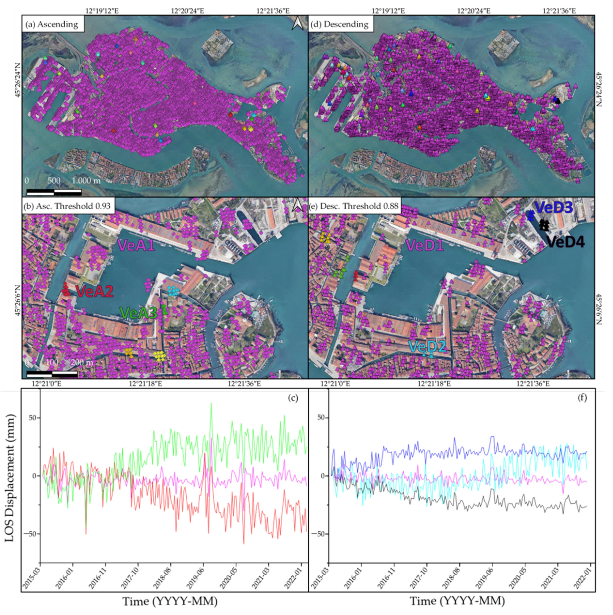
The results of the application of CAPS to the main group of islands of Venice (Figure 13) highlights in both orbits the presence of one large family that includes almost all of the PS. A series of smaller families are dispersed within the main one and referred to single buildings or groups of edifices as shown in Figure 13b,e. For this case, we present only the most appropriate threshold values that are ascending 0.93 and descending 0.88. Figure 13b,e show a further close-up on the eastern sector of Venice where five PS families in ascending mode and four PS families in descending mode have been identified. In Figure 13c,f the time-series of families VeA1, VeA2, VeA3 and VeD1, VeD2, VeD3, VeD4 are shown. The differences in trend between the main family (VeA1/VeD1) and the other families are evident. In particular, in ascending mode the three time-series differ starting from October 2017. This evidence could be compared to the local geophysical or mechanical properties in order to identify the mechanisms controlling the movement in correspondence of the edifices highlighted with CAPS (e.g., foundation instabilities, structural distress). The family distribution can thus help to plan in-depth analyses of specific targets.

4.4. Rome

The analysis at large overview of the metropolitan area of Rome is shown in Figure 14. Even in this case, we conducted two analyses: in the first one we focused on the entire Metropolitan area of Rome considering 1 PS every 65 (in both orbits: total initial PS >1,300,000; remaining PS ~20,000); the second one is focused on Tivoli and surrounding areas considering 1 PS every 5 in ascending mode (Total initial PS >101,000; remaining PS ~20,000) and 1 PS every 6 in descending mode (Total initial PS >115,000; remaining PS ~19,000).

PS maps (Figure 14a,c) show the presence of important subsidence deformations mainly to the west, in the area of Ponte Galeria, and to the east, in the area of Tivoli (see Figure 5). Here, velocities observed along the LOS reach values of −7 to −9 mm/y.

Similarly to the other test sites, PS families identified with CAPS (Figure 14b,d) do not reflect the velocity distribution. Areas characterised by higher velocities are included in macro-families that refer to different behaviours of the surface likely related to different environments. For instance, the green family to the east, very similar in both orbits, could be related to a coastal environment influenced by the delta of the Tiber River. The urban area of the city of Rome is poorly represented probably because of the high presence of heterogeneities. This suggests that, as in the case of Mestre, highly anthropized areas should be analysed with a more local-scale overview.

The analysis of the area of Tivoli through the application of CAPS (Figure 15) shows that the PS in the central part are included in a single family (blue).

This PS family does not reflect the distribution of the velocities suggesting that subsidence could interest an area larger compared to that could be derived from the only velocity distribution. In particular, by overlaying the central family to the lithologic map (Figure 15b,d) it is possible to observe that most of the PS belonging to the central blue family (~60%) are in correspondence of the Travertines (grey) and the Eluvial-colluvial deposits (light green). This agrees with the analyses conducted by [51,52] on the characteristics of the Acque Albule aquifer in Tivoli with different in situ methods. In addition, the blue family also includes PS from the eastern valley where the Aniene River flows from east to west arising new question marks about the dynamics of the area and more specifically, about the geometry and the extension of the aquifer.

As stated before, the aim of this paper is not to explain the causes related to each single family. However, by referring to [4], we can argue that in the area of Rome the subdivision into families is controlled by the variation in geological and hydrogeological characteristics and, more specifically, in the groundwater table geometry and geotechnical properties of the subsoil.

5. Discussion

The method proposed in this paper, CAPS (Correlation Analysis on Persistent Scatterers), proved to be a powerful tool for processing and analysing PSI results. Through a correlation analysis on PS time-series, CAPS allows the identification of groups (or families) of PS showing similar movement over time. The association of a PS to a family is independent of its velocity but only depends on the observed movement in ascending or descending orbit. Therefore, CAPS is also useful to highlight differences in surface deformation in areas that are characterized by similar velocities.

In the examples proposed in the present study for testing the method, CAPS not only allows us to confirm the results of previous studies, but also to provide new findings. For the Santo Stefano d’Aveto and Arzeno landslides, the geographic distribution of the PS families highlights different sectors affected by different kinematics, thus confirming what pointed out by several authors [12,17,24]. For Venice and Rome, the PS family distribution shows macro-areas characterized by similar subsidence movement, but also small areas characterized by small deformation differences (as those highlighted in Venice main island and Tivoli area).

The advantages of the proposed method are twofold. The first benefit is versatility. CAPS can be applied to different geological scenarios. In this paper we have applied it to landslides, which are characterized by significant variation of superficial movement and by complex geological–geomorphological setting, and to subsidence environments, where the deformation rate is lower and less heterogeneous than the previous cases. Moreover, CAPS can work at both large and small scale of observation depending on the purpose of the analysis and/or on the required spatial resolution. It can be used to identify similar environments in terms of ground surface deformation in very large areas (as in Roma and Venice Lagoon test sites), in small areas (as in the main group of islands of Venice, Santo Stefano d’Aveto and Arzeno test sites), or to explain anomalous movements of buildings and infrastructures.

The second benefit is adaptability. As already stated, the identification of PS Families is mainly driven by the value of the cross-correlation threshold used to quantify the similarity between data. On the one hand, such value can be appropriately chosen as a function of the scope of the work and the characteristics of the investigated area. On the other hand, it can be also selected in order to satisfy a priori information. For instance, the value of the threshold can be defined in order to reproduce or confirm findings of previous studies or to point out the deformation in correspondence of specific targets subjected to known movements.

In Appendix A, a comparison table to highlight similarities and differences between each test site is reported.

6. Conclusions

In this research, we proposed a new method, called CAPS (Correlation Analysis on Persistent Scatterers), to analyse time-series of displacement derived from PSI. CAPS is a tool for post-processing ascending and descending PS that groups them into families as a function of the level of similarity of the times series of displacements regardless of the LOS velocity values. This makes it possible to distinguish areas characterized by similar LOS velocity but different ground displacement over time, providing useful constraints for relating the deformations observed at the surface with the geological, geophysical or structural properties of the study area. To this aim, we combined PSI results from both ascending and descending orbits separately with WSA, a procedure generally used in seismology for investigating seismicity patterns. The distribution of the PS families provides information about the kinematics of a targeted area, allowing the identification of sectors with similar displacement. Of note, CAPS can be applied to ascending and descending PS data separately and the comparison between the resulting families can also provide useful information about intrinsic errors and uncertainties in PSI results (due, for instance, to the relative orientation of the satellite respect to the direction of the movement).

The most important parameter that has to be chosen when using CAPS is the value of the cross-correlation threshold, which specifies the level of similarity between two PS time-series. The choice of that value depends on:

-

the focus of the study (e.g., highlighting structural anomalies of single edifices, heterogeneities within a landslide body or different environments in extended areas);

-

the characteristics of the investigated area or phenomena (e.g., orientation compared to the LOS; geological, geotechnical or geophysical heterogeneities that drive kinematics and dynamics of the area);

-

the scale of the investigated area or phenomena (e.g., local or regional)

-

the characteristics of the PS dataset (e.g., number and distribution of PS).

In the application presented in the foregoing, we have provided useful suggestions to choose the value of the threshold as a function of the characteristics of the investigated area or phenomena. When dealing with landslides characterized by high spatially variable deformation rates (>15 mm/y), which are generally related to highly heterogeneous geomorphology as well as complex kinematics and dynamic features, the best threshold value should be sought for the interval 0.85–0.90. Since landslides often develop in little anthropized areas, where few numbers of PS can be extrapolated, the use of relatively low thresholds allows maintaining a sufficient number of PS to be grouped in families. When dealing with areas characterized by low spatial heterogeneities and low displacements such as subsidence environments (absolute LOS velocity, generally, lower than 10 mm/y) the most appropriate threshold should be chosen in the interval 0.90–0.95 or even higher. These are often spatially extended areas where the ground movements are generally related to geological and hydrogeological properties, variations in the groundwater table, and geotechnical characteristics of the subsoil. In these cases, a very large number of PS can be extrapolated and, even using very high threshold values (e.g., 0.98), a sufficient number of PS is maintained at the end of the analysis, thus making possible the identification of subtle differences. Finally, when focusing attention on single buildings, infrastructures or small areas where the deformation is related to local geotechnical proprieties of soil foundations and/or structural distress, the thresholds should be set around 0.90. Obviously, a more helpful guide to setting the most appropriate value of the cross-correlation threshold may be compiled in the future by applying the CAPS tool to many other case studies (also considering the application of CAPS to active volcanoes or glaciers). This will also be helpful to better relate the identified PS families to the geological and geophysical properties that control the ground deformation.

Another benefit of this method is that, when grouping PS into a limited number of families, the analysis of the movement observed at each PS become much simpler. For each family, the analyst can select a reference PS whose time-series can be analysed and compared to the others in order to highlight changes over time in the deformation rate of each homogeneous sector.

To summarise, CAPS has been proven to be a powerful tool for gathering a better interpretation of the deformation maps derived from PS observations. The identified PS families can be related to the differences in terms of ground displacement in areas subject to movement, such as landslides or subsidence, and can be used for identifying the geological and geophysical properties that lead to that deformation. We have shown that the number of families depends on the value of the cross-correlation threshold, whose setting is crucial. Even if the suggestions provided in this study can be helpful for future applications, a trial-and-error procedure is still the best way to determine its value. When increasing the threshold, the total number of PS grouped into families decreases as well as the number of PS in each family, while the number of families tends to increase. Hence, the “best” value should lead to a compromise between the number of families and their population in terms of number of PS. In addition, when geological and geophysical information of the area under study is available, the spatial distribution of the PS families obtained by varying the value of the cross-correlation threshold should be compared to such information. This comparison can thus provide important constraints to identify homogeneous sectors characterised by similar geological and geophysical properties (which determine their displacement) such as depth of the water table, morphology, subsoil geotechnical properties, and geo-lithological composition.

Obviously, CAPS does not allow us to overcome the intrinsic uncertainties of the PSI method (and of InSAR in general) related to the viewing geometry. This remains a crucial parameter that can have a huge impact on the PSI results. The more the real ground movements are perpendicular to the LOS, the more they are underestimated. The viewing geometry also affects the final value of the cross-correlation threshold chosen for the ascending or the descending orbit. As an example, in our landslide test sites (that are better viewed in descending mode due to their orientation), a higher threshold value for the ascending orbit was adopted in order to achieve a distribution of PS families similar to that obtained with the descending orbit.