Forty Years of Wetland Status and Trends Analyses in the Great Lakes Using Landsat Archive Imagery and Google Earth Engine

Abstract

Wetlands provide many benefits, such as water storage, flood control, transformation and retention of chemicals, and habitat for many species of plants and animals. The ongoing degradation of wetlands in the Great Lakes basin has been caused by a number of factors, including climate change, urbanization, and agriculture. Mapping and monitoring wetlands across such large spatial and temporal scales have proved challenging; however, recent advancements in the accessibility and processing efficiency of remotely sensed imagery have facilitated these applications. In this study, the historical Landsat archive was first employed in Google Earth Engine (GEE) to classify wetlands (i.e., Bog, Fen, Swamp, Marsh) and non-wetlands (i.e., Open Water, Barren, Forest, Grassland/Shrubland, Cropland) throughout the entire Great Lakes basin over the past four decades. To this end, an object-based supervised Random Forest (RF) model was developed. All of the produced wetland maps had overall accuracies exceeding 84%, indicating the high capability of the developed classification model for wetland mapping. Changes in wetlands were subsequently assessed for 17 time intervals. It was observed that approximately 16% of the study area has changed since 1984, with the highest increase occurring in the Cropland class and the highest decrease occurring in the Forest and Marsh classes. Forest mostly transitioned to Fen, but was also observed to transition to Cropland, Marsh, and Swamp. A considerable amount of the Marsh class was also converted into Cropland.

1. Introduction

Wetlands provide many services to the environment and humanity, including water purification, protection from natural hazards, soil and water conservation, and shoreline protection [1]. Moreover, wetlands are capable of significant water storage, serve as a form of natural flood control [1], transform and retain chemicals [2,3], and provide habitat for many species of plants and animals [4].

Wetlands are degrading in the world at a fast pace [5,6]. These valuable natural resources are being affected by urbanization, irrigation, climate, pollution, and other anthropogenic activities [5,7,8]. Thus, their ecological functions are negatively influenced, resulting in habitat loss and biodiversity reduction [8]. For instance, Ref. [9] reported that more than 50% of wetlands in North America and Europe are degraded. In Canada, this trend is similarly observed and is expected to continue in the future [10]. However, it is challenging to accurately estimate the extent and type of wetland loss using traditional ground-based approaches. An alternative approach to assessing large-scale wetland changes over time is through remote sensing methods [5,6].

Numerous remote sensing systems capture consistent repetitive imagery with global coverage. Satellite datasets have frequently been used to map wetlands across Canada and have proved to have a high potential to delineate various wetland types [7,11,12,13,14,15,16,17], as well as monitor wetland changes [5,6,18]. For example, optical satellite imagery is commonly used for wetland mapping due to its ability to distinguish spectral differences in wetland species [19]. In this regard, Landsat imagery in particular also provides a historical record of earth observation data from 1972 to the present, allowing for the monitoring of wetland changes occurring over past decades, particularly where field data have not been consistently collected.

Satellite imagery has become increasingly accessible, along with improved processing efficiency. Until recently, acquiring imagery across large spatial and temporal scales was slow and challenging. However, recent advancements have efficiently allowed the acquisition of multiple sources of imagery for large-scale wetland mapping and monitoring initiatives. For instance, Google Earth Engine (GEE) is a cloud-based platform which provides access to a wide range of earth observation products, including the Landsat historical record. In addition to the availability of pre-processed imagery, several machine learning techniques have been implemented and can be imported and modified by users [20,21,22]. To date, many researchers have used GEE to effectively analyze wetland changes over long periods of time. For example, Ref. [6] mapped wetland changes in Newfoundland, Canada, over a 30-year period using the Landsat historical archive in GEE [6]. Additionally, Ref. [5] employed the Landsat archive to develop a machine learning model in GEE that classified wetlands with approximately >80% accuracy for each class [5]. They also identified the percentage of wetland areas that had undergone changes since 1984 for the province of Alberta, Canada.

The Great Lakes region and its subbasins encompass approximately 765,000 km² across the Canada and United States border and contains important wetland areas. Although the region provides millions of people with fresh drinking water, food, and recreational opportunities, it is highly impacted by human disturbances and subsequent wetland loss. Although multiple wetland mapping initiatives have already been undertaken in the Great Lakes basin (e.g., [23,24]), there has not been a comprehensive assessment of wetland change over the entire basin. For example, a user-friendly interface, named Wetland Extent Tool (WET) was developed within GEE by [23] to classify wetlands in the Great Lakes basin. WET was a semiautomated wetland classification workflow to classify multi-source data (i.e., optical satellite, SAR, and elevation images) using the Random Forest (RF) algorithm. WET used a pixel-based classification approach and, thus, was affected by noise due to within-class spectral variation. Moreover, it only resulted in three general categories of wetland, upland, and open-water, and did not include wetland subclasses (i.e., Bog, Fen, Marsh, and Swamp) which are common in Canada and the US. In another study [24], dynamic changes in wetlands, surface water extent, and water level change of wetlands in a portion of the Great Lakes were monitored between 2016 to 2018 using SAR, multispectral, elevation, and InSAR products. The authors mapped dynamic surface water and flooded vegetation extent by thresholding the Radarsat-2 HV polarization observations. The water level monitoring was also conducted using InSAR analysis with the C-band HH polarization SAR data. Additionally, they employed a variety of approaches for the classification and change detection of wetlands in the Great Lakes basin, including spatio-temporal classification, Object-Based Image Analysis (OBIA), and SAR-based classification. Although the authors of [24] exhibited promising results for wetland change detection in the Great Lakes basin, it was conducted over a few selected pilot sites and did not extend to the entire basin or multiple decades. Furthermore, such an approach requires high-resolution datasets, which are usually expensive and not freely available.

In this study, we developed a model to examine changes in wetland types and extents in the Great Lakes basin over the past four decades. To this end, advanced classification and Change Detection (CD) algorithms were developed and applied to the archived Landsat imagery within the GEE cloud computing platform. In contrast to the authors of [23], an object-based RF classification was used to generate a more accurate wetland map. Moreover, four wetland classes (i.e., Bog, Fen, Marsh, and Swamp) and five non-wetland classes (i.e., Open Water, Forest, Grassland/Shrubland, Cropland, and Barren) were delineated to provide more detailed wetland maps. Finally, open-access Landsat data were employed to facilitate wetland change analysis over large areas and multi-decade time frames.

2. Materials and Methods

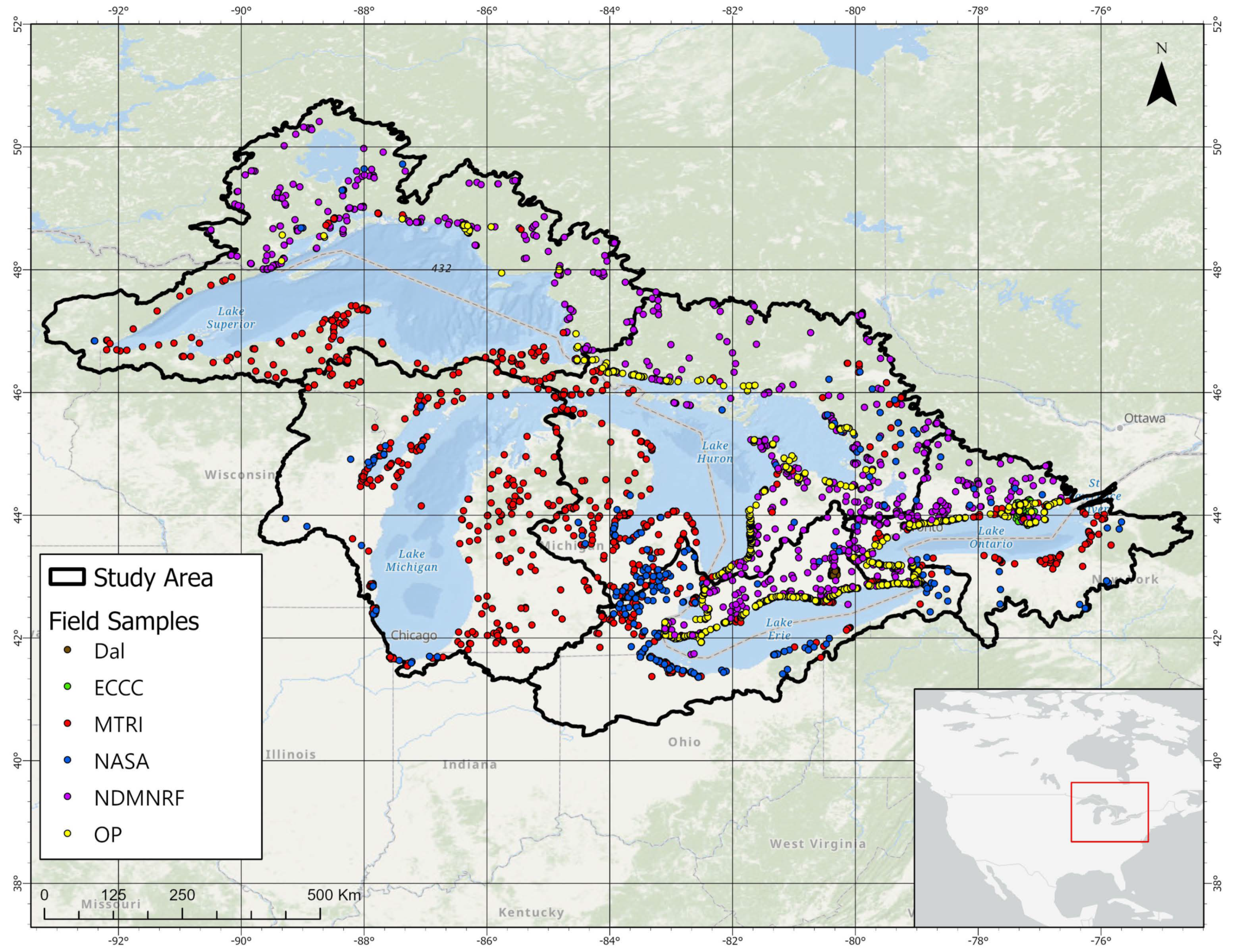
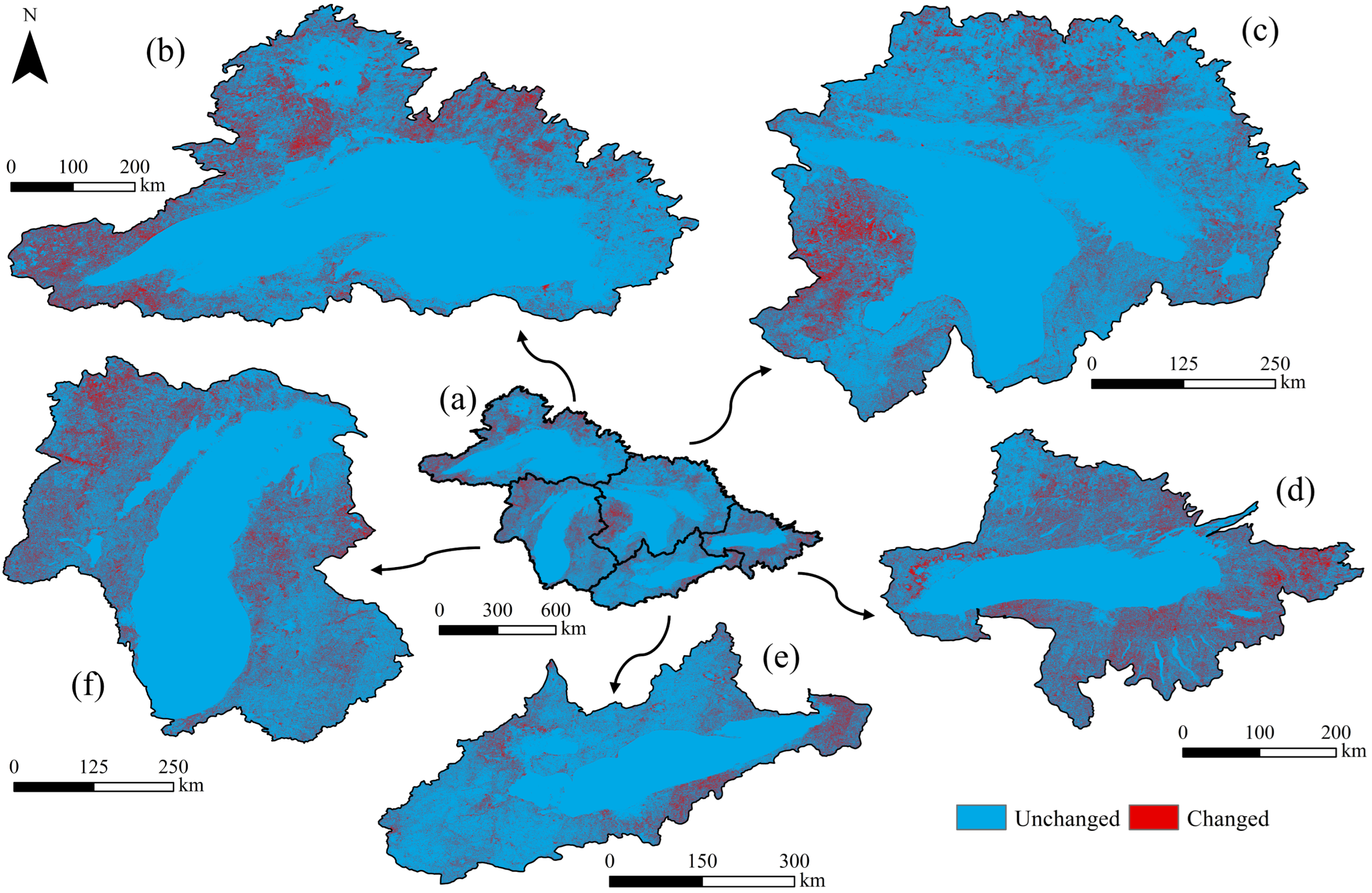
2.1. Study Area

The Great Lakes (Figure 1) are a series of large and interconnected freshwater lakes in central North America, whose individual subbasins form the larger Great Lakes basin and constitute the largest freshwater reserve on Earth. The Great Lakes basin was formed during the recession of the Laurentide ice sheet and now contains diverse ecosystems and abundant plant and wildlife [25,26]. The region spans a large and variable area, but generally hosts a humid continental climate, which can be influenced by air masses from other regions (e.g., cold Arctic air, warm tropical air). Wetlands occur throughout the study area, most commonly in coastal and riverine settings, though they can also be found inland.

2.2. Field Data

Field data were collected and provided by various organizations, including the Michigan Tech Research Institute (MTRI), National Aeronautics and Space Administration (NASA), Dalhousie University (Dal), Environment and Climate Change Canada (ECCC), Ontario Parks (OP), and Ministry of Northern Development, Mines, Natural Resources, and Forestry (NDMNRF). The data provided by MTRI, NASA, Dal, and ECCC were GPS point locations of wetland and non-wetland species collected in the field in the following years, respectively: 2010–2018, 2017–2019, 2012–2013, and 2016. The data provided by OP were landcover polygons derived through photo interpretation by OP’s ecologists in 1989–2001. A portion of the data provided by NDMNRF were collected in the field, with the rest created by photo interpretation and including various information about wetlands and other landcovers from various years between 2016–2019. The distribution of all field samples is illustrated in Figure 1. The samples were well distributed over the Great Lakes basin and, thus, these samples can properly represent different types of wetland and non-wetland classes in the study areas.

Table 1. The statistics of the preprocessed field samples (polygons) received from different organizations.

	MTRI		NASA		Dal		ECCC		OP		NDMNRF
Class	# Polygons	Area (ha)	# Polygons	Area (ha)	# Polygons	Area (ha)	# Polygons	Area (ha)	# Polygons	Area (ha)	# Polygons	Area (ha)	Total #	Total Area (ha)
Bog	59	1125.0	15	112.1	0	0	0	0	16	68.2	11	122.4	101	1427.7
Fen	99	5831.6	17	188.9	0	0	0	0	0	0	30	425.6	146	6446.1
Marsh	695	13,314.7	188	834.6	54	88.7	27	1885.4	0	0	116	1309.2	1078	17,425.6
Swamp	0	0	0	0	48	782.1	13	1736.3	0	0	211	3835.8	272	6354.2
Open Water	155	3775.2	0	0	113	51.0	8	1286.0	0	0	20	226.0	296	5338.2
Forest	43	1043.8	5	46.2	0	0	35	617.9	0	0	472	13,491.6	555	15,199.5
Grassland/Shrubland	0	0	0	0	0	0	0	0	300	1534.2	2	8.2	277	1424.0
Cropland	12	198.6	0	0	0	0	0	0	364	2829.5	4	37.0	380	3065.1
Barren	0	0	0	0	0	0	0	0	59	4368.7	24	116.7	81	4432.4
Total	1062	25,284.6	224	1179.2	215	921.8	83	5525.6	712	8629.0	890	19,572.5	3186	61,112.6

MTRI: Michigan Tech Research Institute, NASA: National Aeronautics and Space Administration, Dal: Dalhousie University, ECCC: Environment and Climate Change Canada, OP: Ontario Parks, NDMNRF: Ministry of Northern Development, Mines, Natural Resources, and Forestry, #: number.

provides information regarding the number and area of the field samples collected and prepared as part of this study. In total, nine landcover classes were considered based on the Canadian Wetland Classification System (CWCS) system and previous wetland studies conducted in Canada and the US: four wetland classes of Bog, Fen, Marsh, and Swamp, as well as five non-wetland classes of Open Water, Forest (e.g., deciduous, coniferous, and mixed woodlands), Grassland/Shrubland, Cropland, and Barren (e.g., urban, rock, bare soil, sand, and other non-vegetated areas). The majority of sample areas belonged to the Marsh and Forest classes, respectively, while the number and area of samples from the Bog and Grassland/Shrubland classes were relatively small. It is worth noting that the Open Water class was composed of both Shallow Water and Deep Water classes. However, due to the low number of Shallow Water field samples and their lower accuracy, it was decided to consider one water class as Open Water.

2.3. Satellite Data

In this study, the archived level 2 products (surface reflectance) of Landsat-5, -7, and -8 images from 1984 to 2021 available in GEE (https://developers.google.com/earth-engine/datasets/catalog/landsat, accessed on 20 January 2022) were employed (

Table 2. The Landsat images used at different time intervals (i.e., two or three years) to produce 17 wetland maps. (The time interval which is bolded was used as the reference interval for change analysis.)

Time Interval Number	Time Interval Range	Landsat-5	Landsat-7	Landsat-8	Number of Images
T1	1984–1986	-			2530
T2	1987–1989	-			2905
T3	1990–1992	-			3033
T4	1993–1995	-			2980
T5	1996–1998	-			2997
T6	1999–2000	-	-		4369
T7	2001–2002	-	-		4602
T8	2003–2004	-			2244
T9	2005–2006	-			2181
T10	2007–2008	-			1829
T11	2009–2010	-			2117
T12	2011–2012		-		3110
T13	2013–2014		-	-	4862
T14	2015–2016		-	-	4868
T15	2017–2018		-	-	4811
T16	2019–2020		-	-	4710
T17	2020–2021		-	-	4361

). In total, 58,509 Landsat images were acquired and processed. As outlined in Table 2, the images from every three-year period (1984–1998) or every two-year period (1999–2021) were combined to produce cloud-free Landsat mosaic images for the entire study area. It should be noted that the study area is covered by clouds and snow for much of the year and creating cloud-free images with less time intervals (T), such as annual images, was not possible. In total, 17 time intervals were considered and, thus, 17 wetland maps were produced to analyze changes over the past four decades.

2.4. Methodology

The employed methodology included four main steps. First, the field data were preprocessed to make them suitable for wetland mapping and change analysis (see Section 2.4.1). Subsequently, all available field samples were analyzed in order to select only spectrally unchanged samples for use in the classifications of all time intervals (see Section 2.4.2). Then, the selected samples were used to train the classification algorithm and produce wetland maps at different time intervals (see Section 2.4.3). Finally, a CD algorithm was applied to assess wetland trends over the past four decades (see Section 2.4.4).

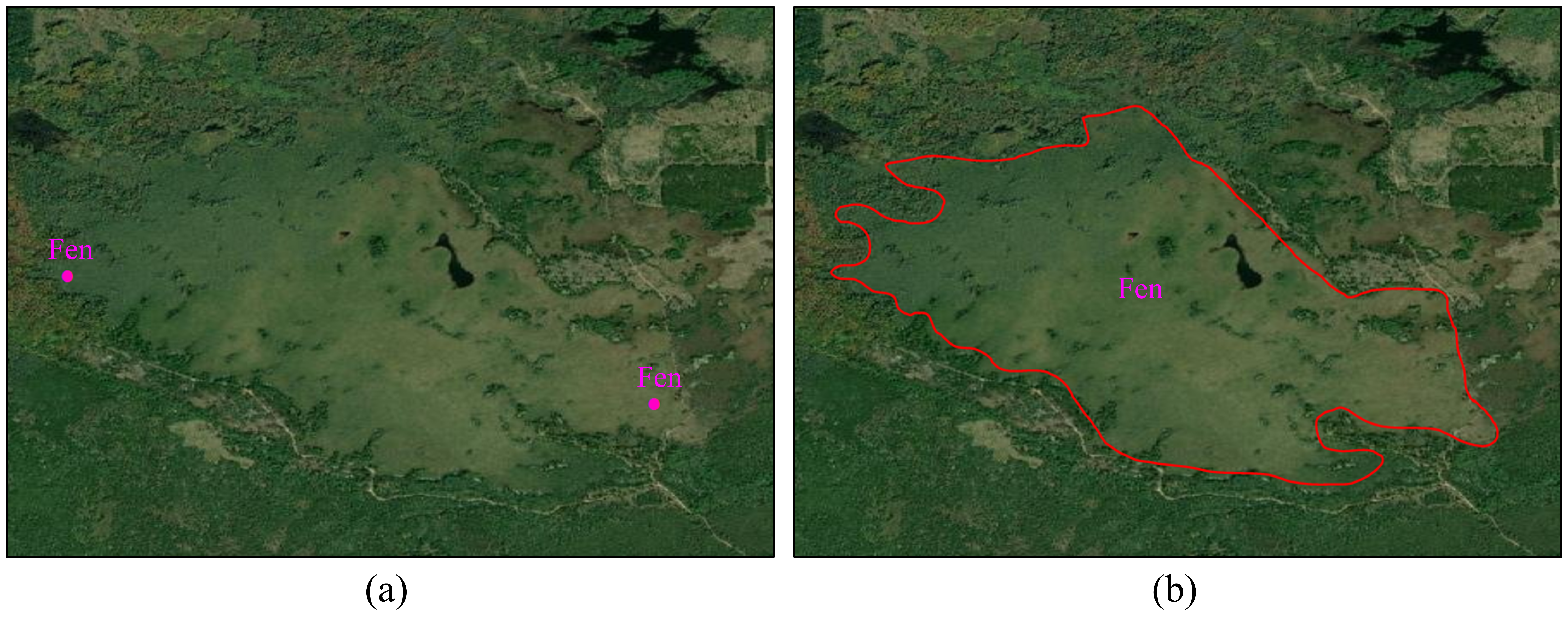
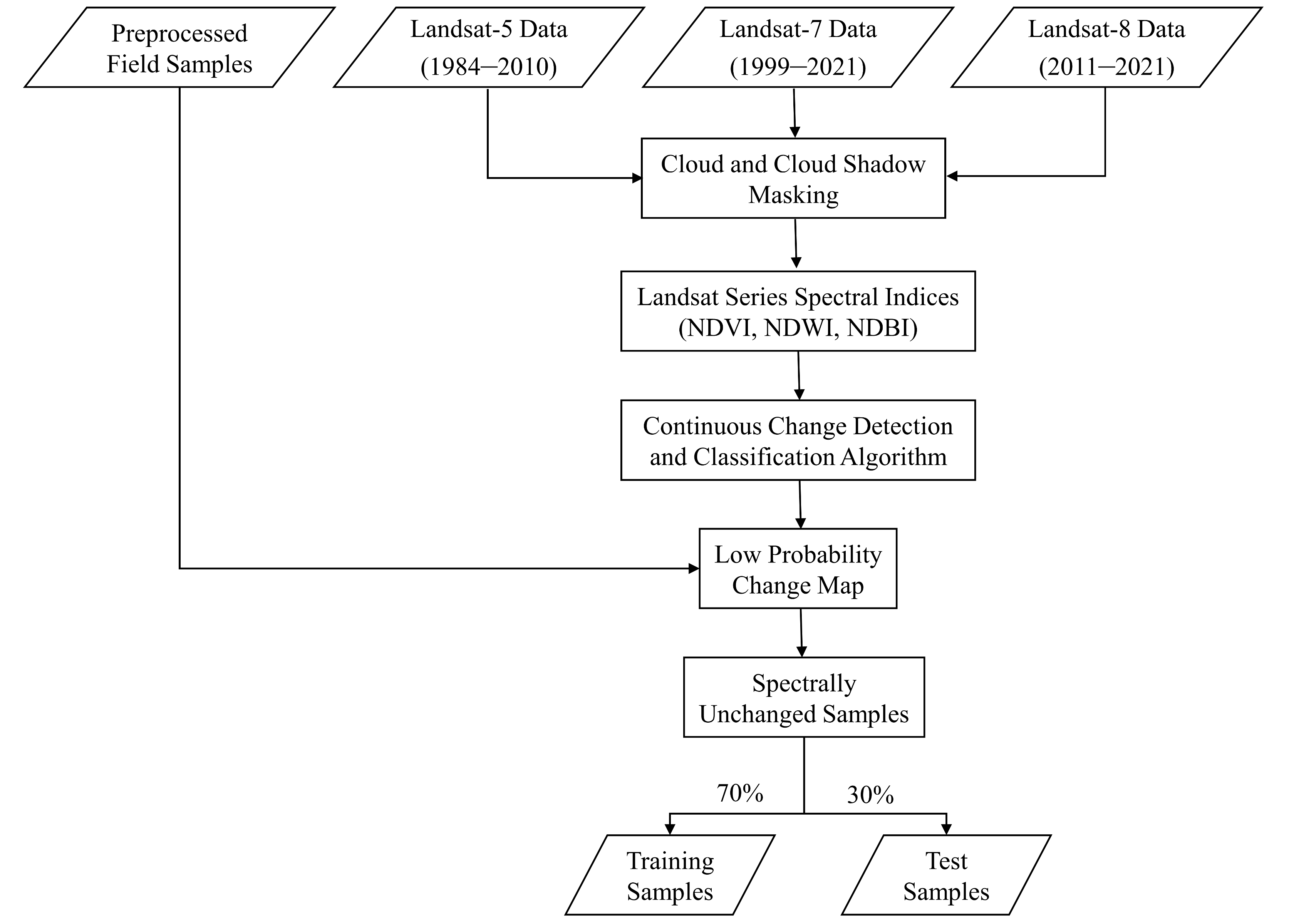
2.4.1. Field Data Preparation

The point-based samples were used to delineate the corresponding site boundaries using high-resolution satellite images available in Google Earth and ArcGIS (see Figure 2 for an example). Delineated polygons were subsequently reassessed for accuracy (in terms of both location and extent) before being included in the classification model.

2.4.2. Unchanged Field Samples Selection

The flowchart of the method to generate spectrally unchanged field samples is illustrated in Figure 3. In this study, the Continuous Change Detection and Classification (CCDC; [27]) method was utilized to select unchanged samples and generate additional field samples for each time interval when field data had not been collected during those years. The CCDC method analyzes all field samples and selects the samples whose spectral responses have remained unchanged over the study period; in this case, four decades. The resultant samples are referred to as the unchanged field samples and used as training and test data for all years.

First, cloud, cloud shadow, and snow/ice pixels were masked in the Landsat images using the quality band of Landsat (i.e., Bitmask for pixel_qa) and C Function of Mask (CFMASK) algorithm [28] within GEE. The quality band flags undesired pixels (e.g., cloud and snow) with a class name or unused designation, depending on the Landsat generation [29]. The masked Landsat images were then applied to calculate three spectral indices, Normalized Difference Vegetation Index (NDVI, Equation (1)), Normalized Difference Water Index (NDWI, Equation (2)), and Normalized Difference Build-up Index (NDBI, Equation (3)), which were then used to determine the unchanged field samples using the CCDC model derived in Equation (4).

$$NDVI=\frac{NIR-RED}{NIR+RED}$$

(1)

$$NDWI=\frac{GREEN-NIR}{GREEN+NIR}$$

(2)

$$NDBI=\frac{SWIR-NIR}{SWIR+NIR}$$

(3)

$$F\left(i,x\right)=a_{0,i}+a_{1,i}\cos \left(\frac{2\pi }{t}x\right)+b_{1,i}\sin \left(\frac{2\pi }{t}x\right)+c_{1,i}x$$

(4)

where i, x, and t, respectively, indicate the spectral index, Julian date, and the number of days per year (i.e., 365.25 days); $a_{0,i}$ stands for the overall value of the spectral index i of a Landsat image; $a_{1,i}$ and $b_{1,i}$ specify the intra-annual change; and $c_{1,i}$ shows the interannual change. The model coefficients were determined from the field samples. The new samples were inserted into Equation (4) to estimate model values and residuals by comparing the observed and modelled sample values. A threshold value was set to 20%, where it was assumed that an abrupt or interannual change had occurred if residuals exceeded 20%. Samples that did not meet the threshold were not used in the classification of another time interval. The final remaining samples were assumed to have stable spectral responses and therefore had not undergone change over the study period. As such, these samples were used to classify wetlands for all 17 intervals. Prior to classification, the unchanged field samples were randomly split into training (70%) and test (30%) groups, where the training group was used to train the classification algorithm and the test group was used to assess the accuracy of the resultant wetland maps.

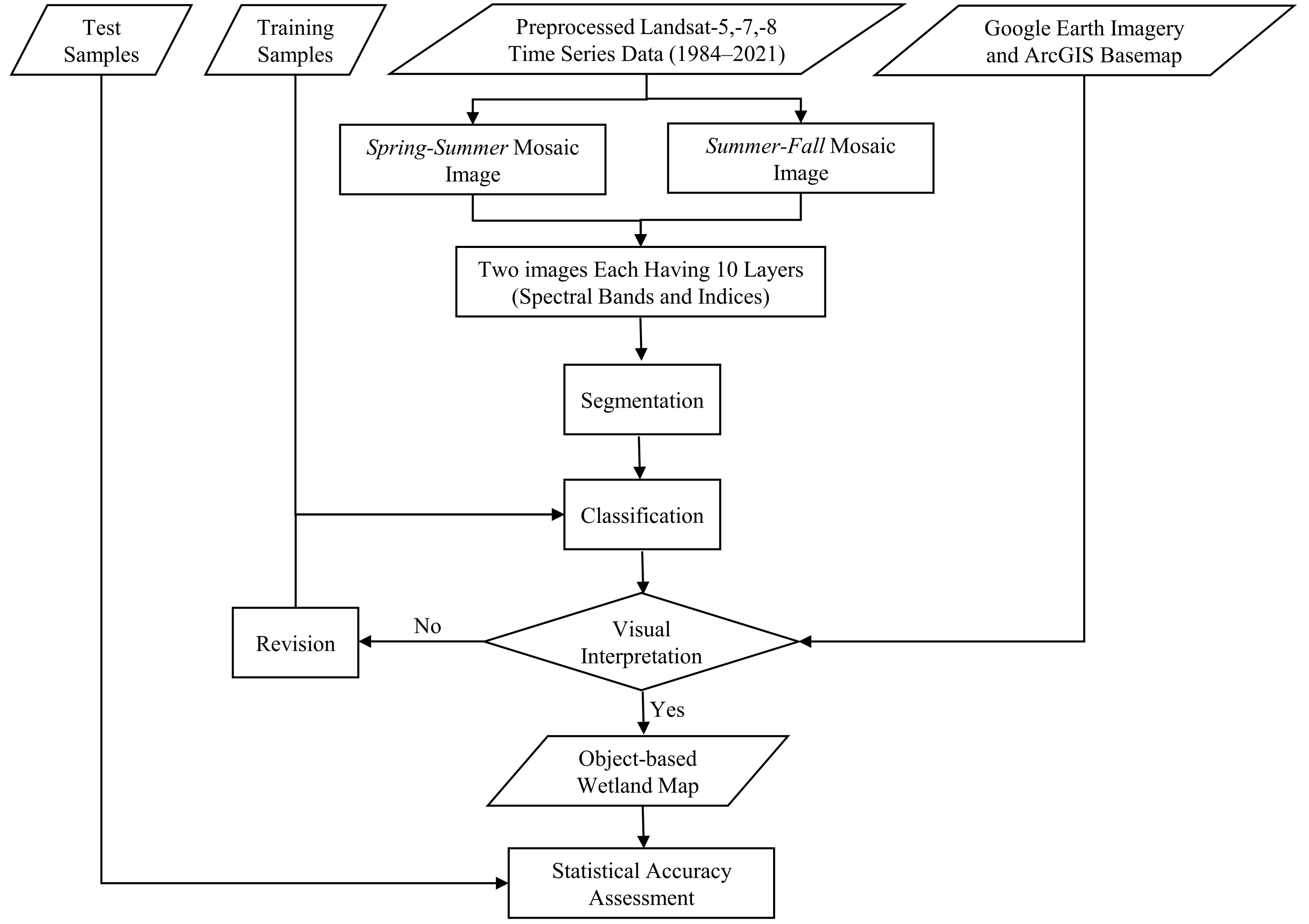
2.4.3. Classification

The steps of the classification method to produce wetland maps at different time intervals are demonstrated in Figure 4.

Wetlands maps for each time interval were generated using the unchanged field samples identified through the CCDC process. Cloud, cloud shadow, and snow/ice were masked from all images, which were then divided into two groups based on season: (1) the months of April, May, June, and July, which was called the Spring–Summer time, and (2) the months of August, September, and October, which was called the Summer–Fall time. The reason for this was because it has been widely reported that multi-temporal datasets could improve wetland detection [7,13,30]. All images within each group were then down-sampled into a single mosaic by calculating the mean value per pixel over the entire time series (i.e., the Spring–Summer and Summer–Fall mosaic images). Ten features (layers), which included the seven main spectral bands of Landsat images (i.e., blue, green, red, Near Infrared (NIR), two Shortwave Infrared (SWIR), and Thermal Infrared (TIR) bands), and the three spectral indices (NDVI, NDWI, and NDBI) were extracted from each mosaic image and used in the classification.

Object-based classification techniques have been widely reported to produce better results when compared to pixel-based methods [13,30,31]. Additionally, large heterogeneous landcover types, such as wetlands, have been shown to require an object-based approach [11]. Therefore, the mosaicked images were ingested into the Simple Non-Iterative Clustering (SNIC) algorithm to be segmented. The SNIC method evenly distributes a number of seeds throughout the image to partition it into super-pixels. A priority queue is then applied to determine the next pixel to be assigned to a cluster based on the distance of the pixel from the segment centroid. After each new pixel is added to a cluster, a new centroid is computed. This process continues until centroid convergence [32].

The final segmented image, consisting of 20 layers (i.e., 10 layers from each of the Spring–Summer and Summer–Fall mosaic images), was ingested into an RF classification algorithm. RF has proven to be an effective classifier for landcover classification, especially for wetland mapping [7,13,30,33]. RF contains a set of decision trees that divide the input pixels into mutually exclusive groups until each node represents one of the final classes. Model tuning parameters are selected based on the available samples and the objectives of the classification. In this study, these parameters were selected after several trial-and-error classification iterations and based on the results of previous wetland mapping studies within GEE [5,34,35]. Accordingly, the following values were selected for each tuning parameters of the RF algorithm: numberOfTrees = 50, variablesPerSplit = 5, minLeafPopulation = 1, and bagFraction = 0.5.

• Accuracy assessment

After the classification was conducted, it was visually assessed using Google Earth high-resolution images and basemaps available in ArcGIS. If the visual inspection suggested the classification could be further improved, the classification parameters and/or the training samples were revised, and the RF retrained until satisfactory results were obtained. For the statistical accuracy assessment, the final classification was compared with the test data and the results presented in a confusion matrix. The confusion matrix was used to examine whether different classes in the generated wetland maps were confused with other classes.

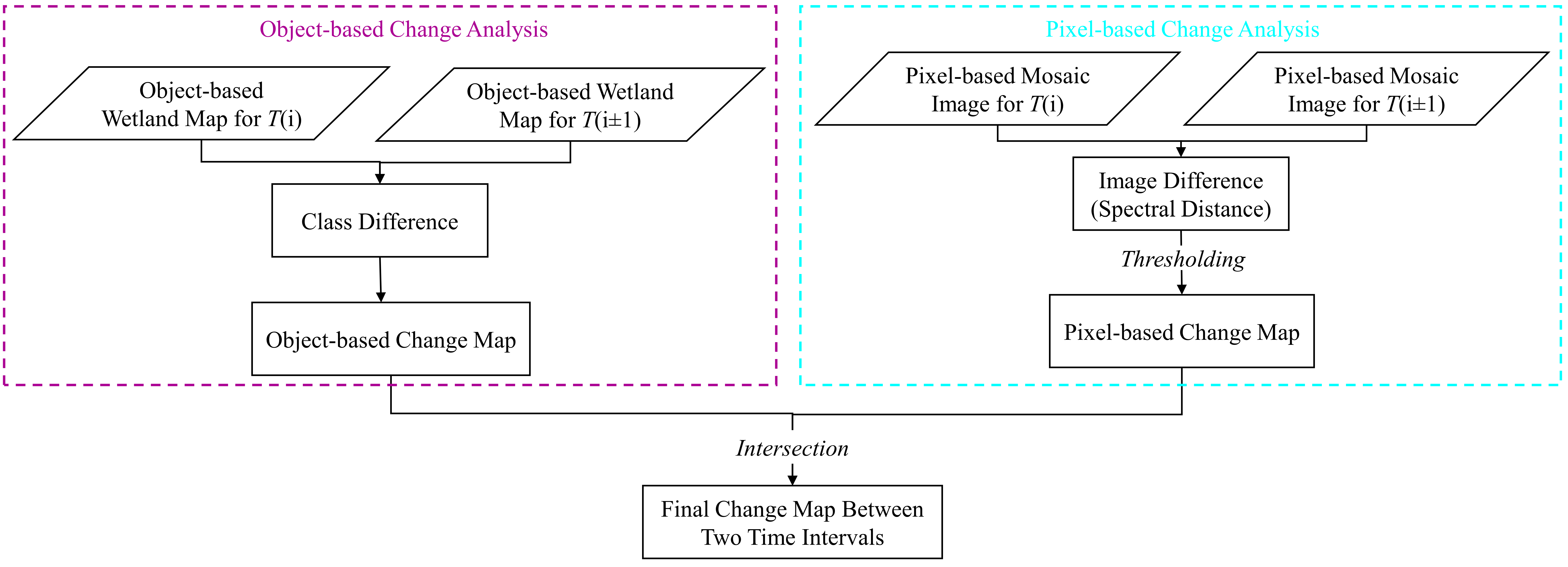
2.4.4. Change Detection (CD)

Change analysis was conducted using the 17 produced wetland maps, where the map produced for 2020–2021 (T17 in Table 2) was selected to be the reference time interval as it covered the most recent time interval and achieved the highest map accuracies. It should be noted that the selection of the reference interval does not significantly affect the analysis and is simply a starting point for the CD algorithm.

• Change Detection (CD) between two time intervals

The differences between every two time intervals were first determined using two CD methods of class differencing and image differencing (see Figure 5). The combination of the two methods improved CD results as opposed to only using a single method. Furthermore, utilizing pixel- and object-based CD methods decreased the overestimation of changed areas and noise, respectively.

The pixel-based change analysis was conducted using the spectral bands of the Spring–Summer and Summer–Fall mosaic images, where the spectral distance between the mosaicked images of two time intervals was calculated. A threshold of 70% was subsequently applied to the resultant map, where a difference greater than 70% between the spectral responses of pixels at two different time intervals indicated changed pixels. The object-based change analysis was conducted by differencing two object-based wetland maps. The final change map was produced as the intersection of the pixel- and object-based change maps, where the final change map was object-based.

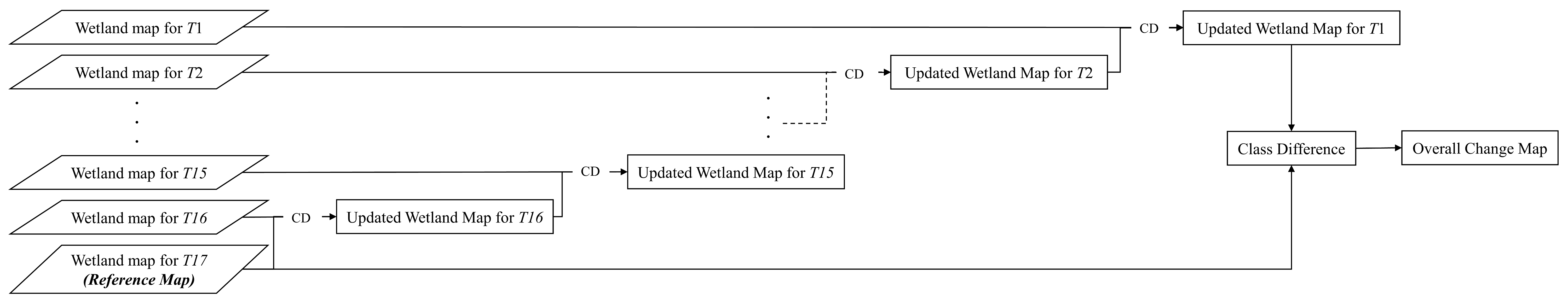
• Change Detection (CD) through all time intervals

As the main objective of this study was to analyze the changes occurring over the past four decades, an additional analysis was conducted (see Figure 6) to determine overall wetland changes occurring during the past 40 years. First, using the reference map (i.e., T17) as one of the two change analysis maps, the other map (i.e., T16) was updated. Specifically, the class labels of the changed objects in the other map were updated based on the reference map class labels. Through this approach (Figure 6), all 16 other maps were hierarchically updated, and the overall changes were determined.

3. Results and Discussion

3.1. Classification

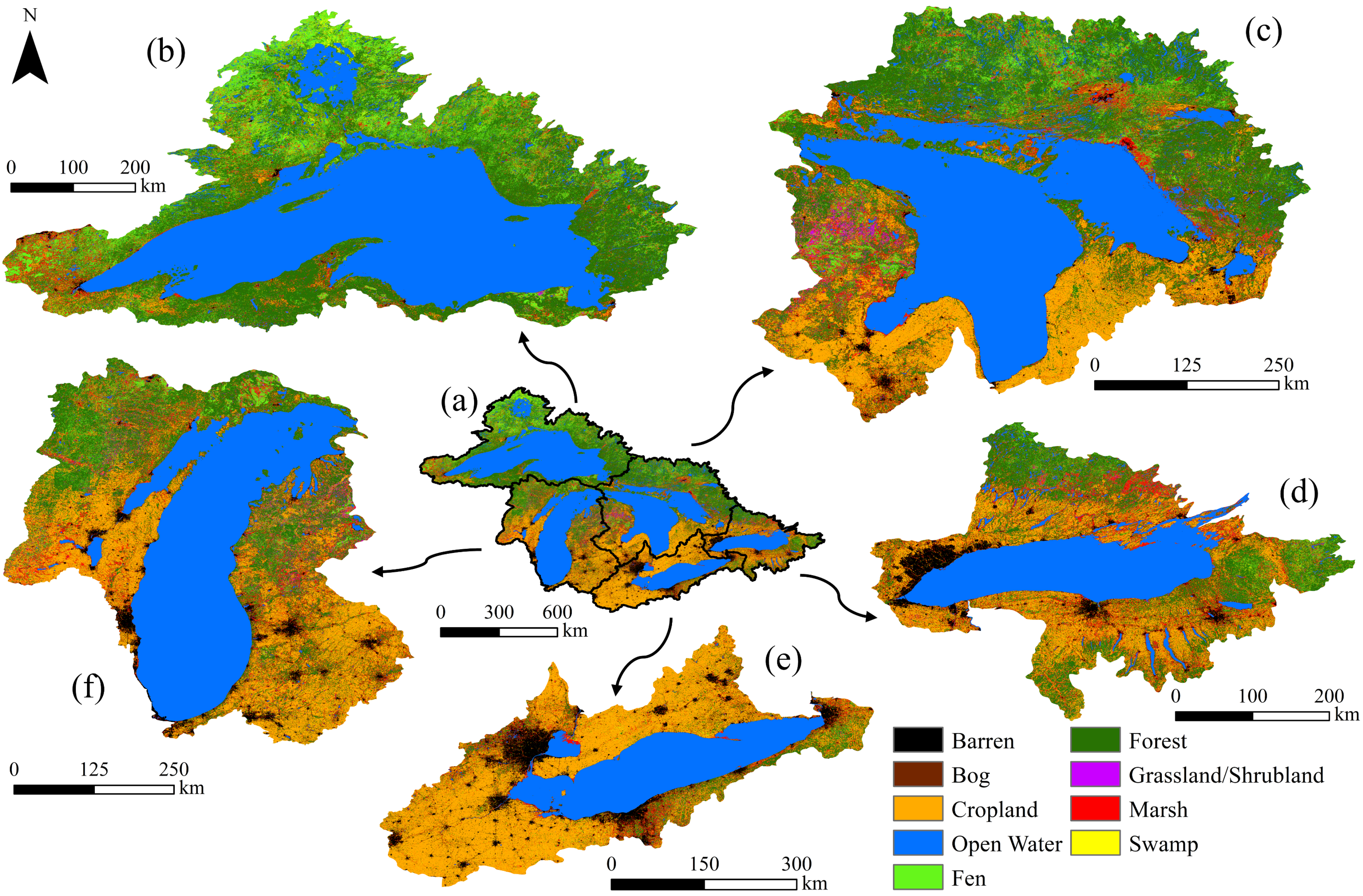
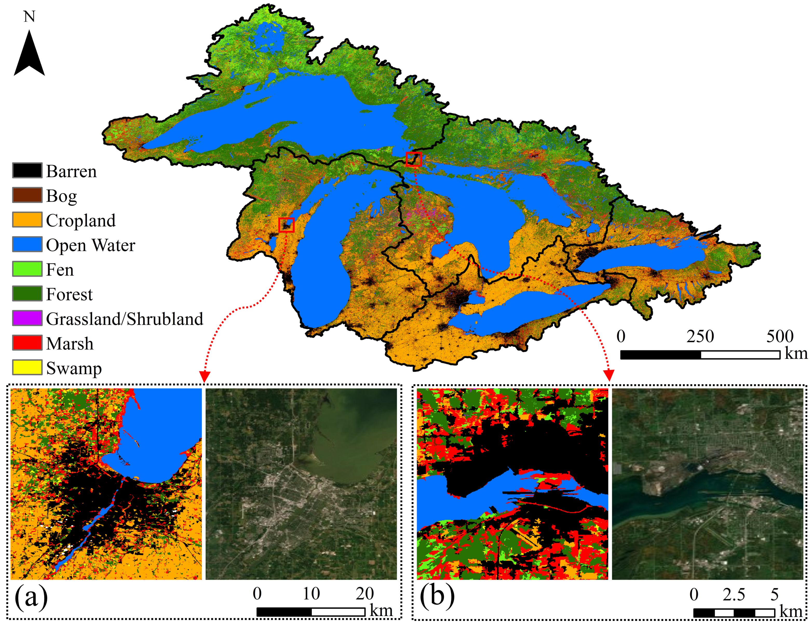
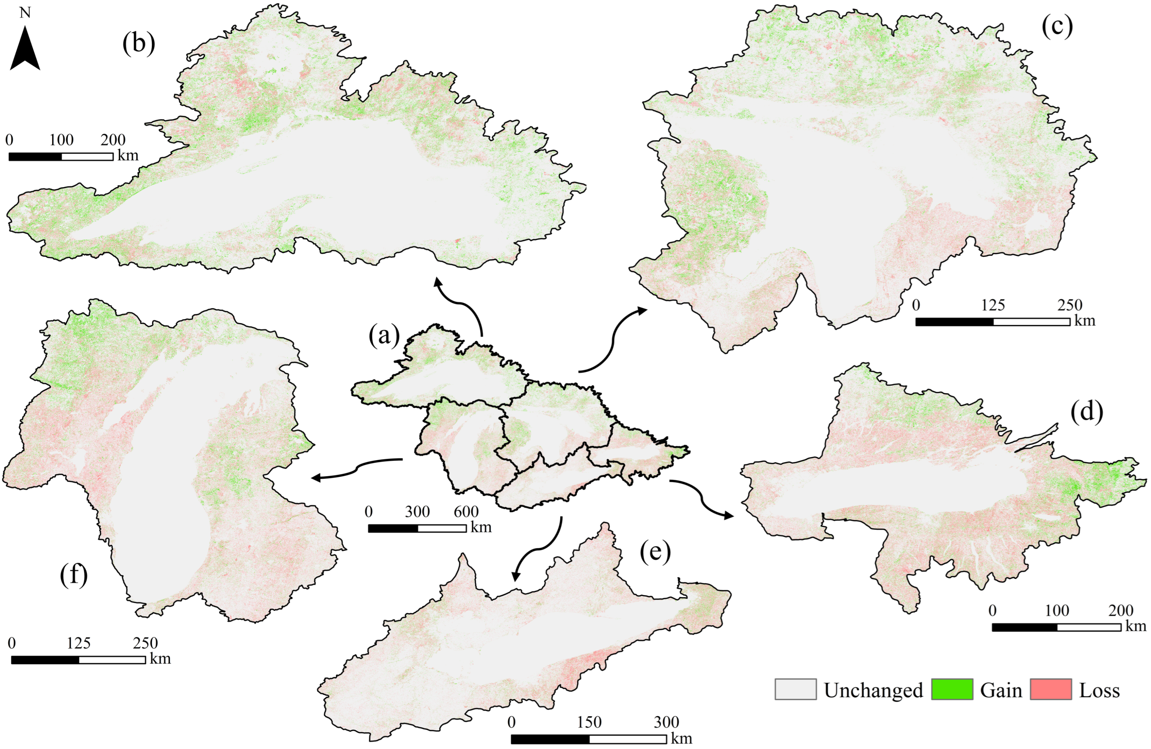
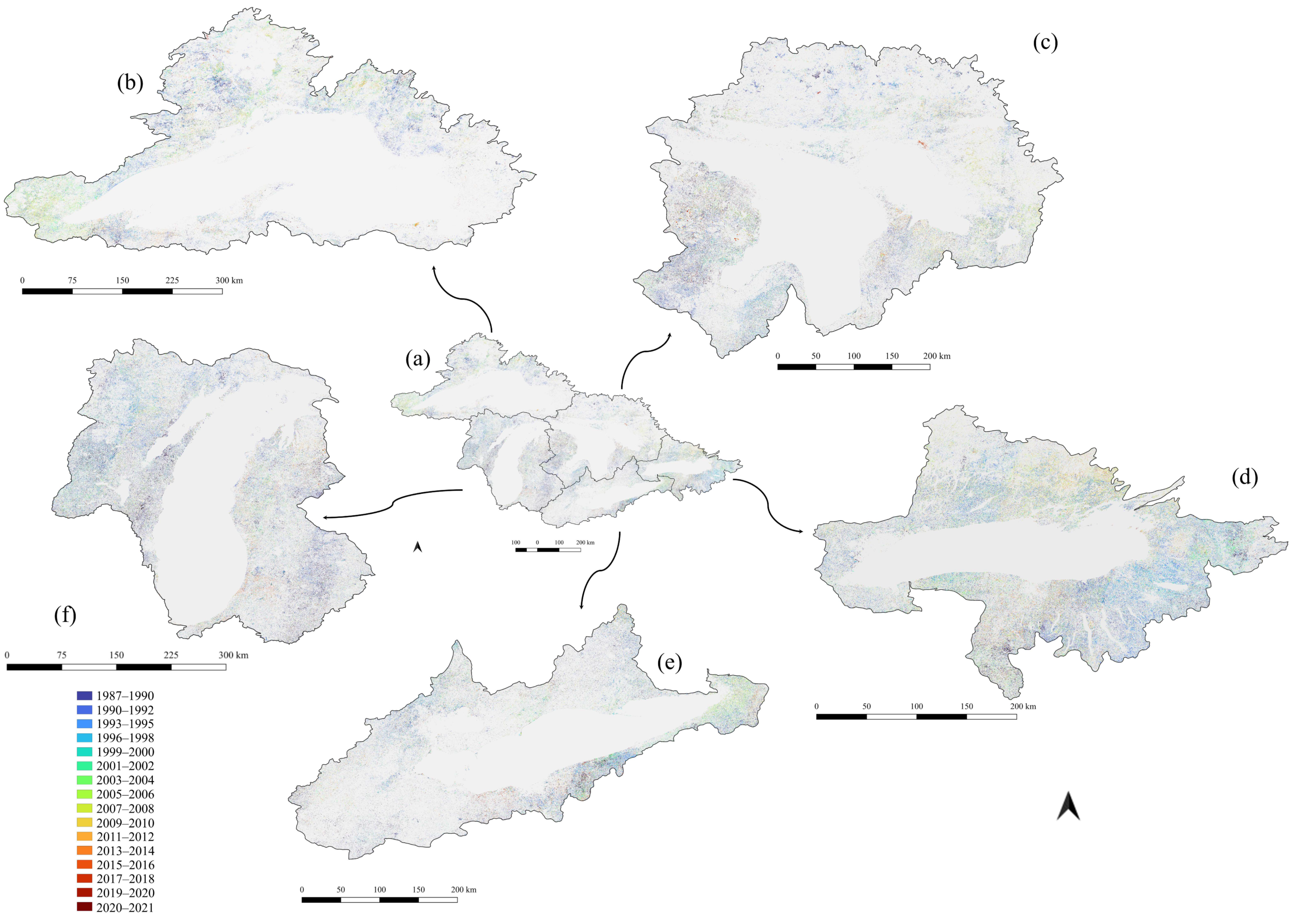
3.1.1. Classified Maps

After preparing field samples for all time intervals (see Section 2.4.1 and Section 2.4.2) to support the supervised classification task, wetland maps were generated for 17 time intervals between 1984 and 2021 based on the methods discussed in Section 2.4.3. Figure 7 presents the generated wetland map of the reference time interval (i.e., 2020–2021) for the entire Great Lakes basin and its five subbasins individually.

Visual inspection of the produced wetland maps showed satisfactory accuracy in identifying different wetland and non-wetland classes. For example, the method accurately delineated large water bodies and urban areas as Open Water and Barren. Additionally, the southern portions of the Great Lakes basin, which are dominated by agricultural lands, were correctly identified as Cropland. The quantitative values extracted from the reference wetland map indicated that the study area is mainly covered by Open Water (34.8%), Forest (24.6%), and Cropland (17.7%), respectively. On the other hand, Bog (0.003%), Grassland/Shrubland (0.7%), and Swamp (1.25%) were the classes that covered the least amount of area within the Great Lakes basin. Further visual investigations at subbasin levels also suggested that the methodology was capable of capturing smaller water bodies and urban areas.

Visual intercomparisons using high-resolution satellite images were also carried out to assess the quality of the produced wetland maps at smaller scales. Two zoomed-in classified areas, along with their corresponding high-resolution satellite imagery, are demonstrated in Figure 8. Based on Figure 8a, the implemented approach correctly distinguished different land covers. For example, the agricultural lands outside and surrounding metropolitan areas were correctly identified as Cropland. Likewise, the urban areas, water bodies, and forest patches were also accurately assigned to Barren, Open Water, and Forest, respectively (see Figure 8b). Considering both zoomed-in patches, several pixels located around large water bodies and multiple small shallow water areas were also correctly classified as Marsh (i.e., emergent marshes), which was also observed in other parts of the produced wetland maps.

Despite the high visual accuracy of the maps, there were errors, such as the misclassification of Forest as Swamp and incorrect classifications of Cropland as Grassland/Shrubland or other wetland classes. The confusion between the Forest and Swamp classes has been reported in many other wetland mapping studies [5,36]. Swamp and Forest have similar spectral responses in optical satellite imagery; thus, it is challenging to separate these two classes when only optical data are employed [36]. Other remote sensing datasets, such as L-band Synthetic Aperture Radar (SAR) data, are required to better discriminate between these two classes.

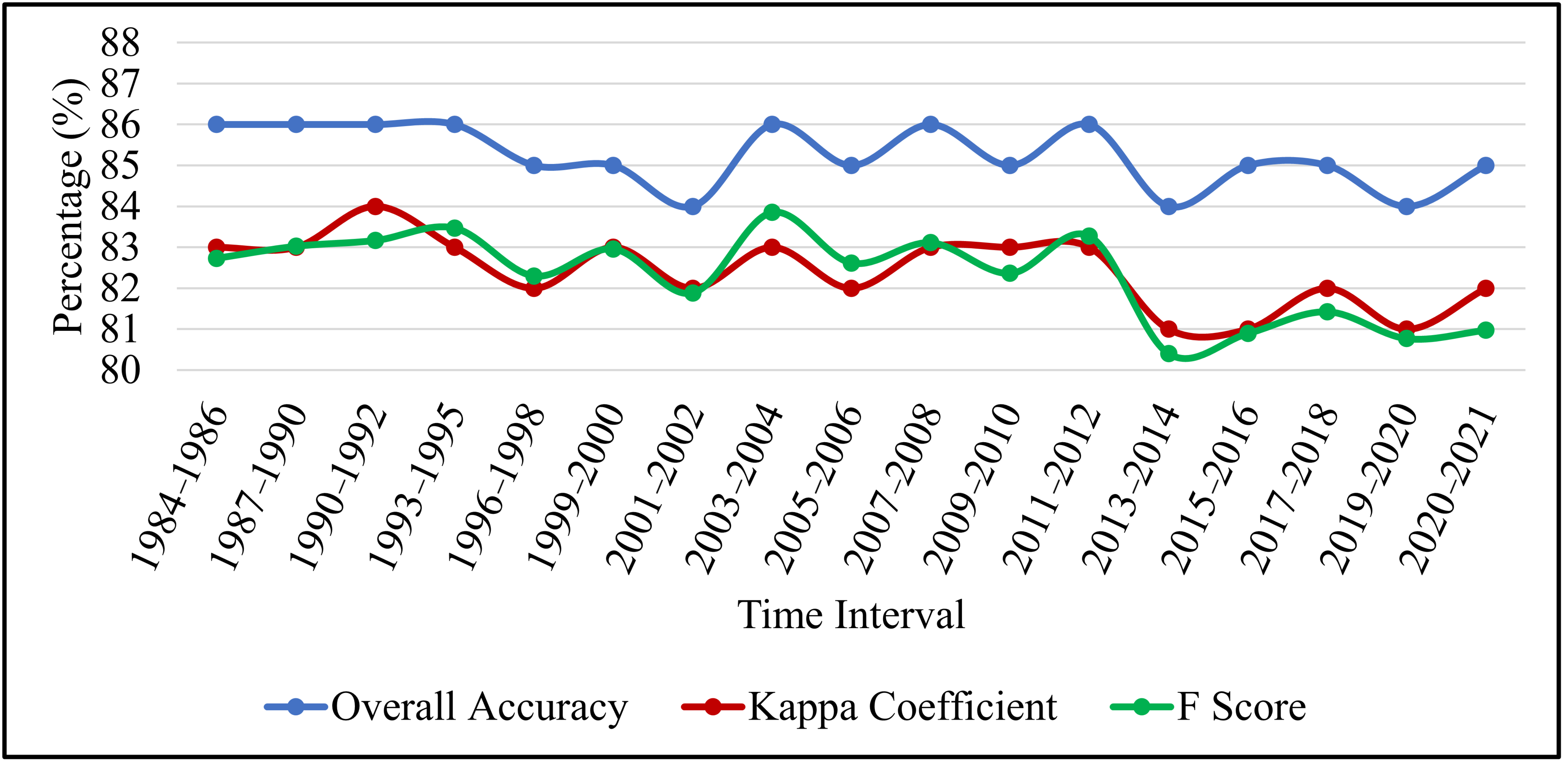
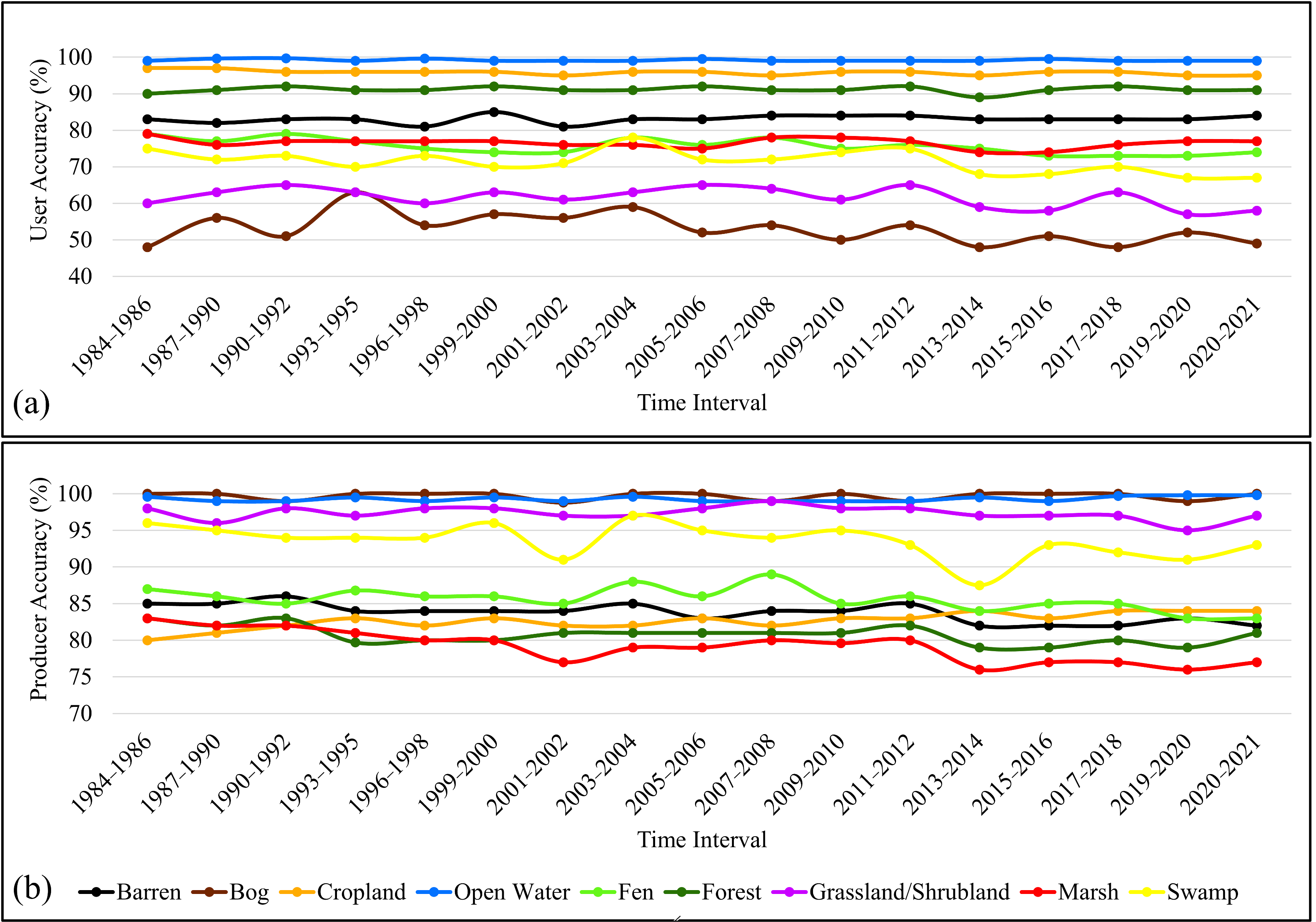
3.1.2. Accuracy Levels

In addition to the visual evaluation of all wetland maps, independent test samples (30% of field data) were employed to quantify the accuracy of each generated wetland map by calculating a confusion matrix. As illustrated in Figure 9, all of the wetland maps had OAs and KCs greater than 84% and 81%, respectively, indicating the high potential of the proposed methodology for large-scale wetland mapping using only spectral indices derived from optical satellite data. The low variation in the obtained OAs (85.2% ± 0.7%) and KCs (82.4% ± 0.8%) also demonstrated the consistent performance and robustness of the applied classifier. As is clear in Figure 10, the average UAs of all wetland maps were between 76.6% and 80.3%, with the lowest and highest average UAs belonging to wetland maps of the 13th (i.e., 2013–2014) and 8th (i.e., 2003–2004) time intervals, respectively. In terms of the class-wise UAs, Open Water and Cropland obtained the two highest UAs in all time intervals with average UAs of 99.1% and 95.8%, respectively, followed by Forest, Barren, Marsh, Fen, Swamp, Grassland/Shrubland, and Bog. Bog acquired the lowest UAs in almost all time intervals, except for the 4th time interval, with UAs between 48% and 57%. However, Bog had higher PAs in most time intervals in comparison to other classes, leading to average PAs of approximately 99.6%. Open Water and Grassland/Shrubland had the second- and third-highest PAs with average values of 99.2% and 97.3%, respectively. The lowest PAs were recorded for Marsh in almost most of the generated wetland maps, with an average PA of 79.1%. Overall, the average PAs were relatively higher than the average UAs, commencing at 87.6% in the 13th (i.e., 2013–2014) time interval and peaking at 90.1% in the 1st (i.e., 1984–1986) time interval.

The confusion matrices for all wetland maps were also calculated. As an example,

Table 3. Confusion matrix of the generated wetland map of the Great Lakes basin using Landsat imagery and Random Forest (RF) algorithm for the reference time interval (i.e., 2020–2021).

		Field Samples
		Barren	Bog	Cropland	Open Water	Fen	Forest	Grassland/Shrubland	Marsh	Swamp	Total
	Barren	1095	0	101	0	12	12	1	76	1	1298
	Bog	5	74	9	0	22	11	1	28	1	151
	Cropland	29	0	2116	0	4	9	2	67	1	2228
Classified	Open Water	1	0	0	1225	2	0	0	6	0	1234
	Fen	42	0	77	0	910	80	1	108	5	1223
	Forest	8	0	7	1	43	1191	0	48	4	1302
	Grassland/Shrubland	22	0	38	0	18	33	245	63	4	423
	Marsh	123	0	163	2	63	66	3	1383	4	1807
	Swamp	6	0	3	0	23	77	0	20	263	392
	Total	1095	0	101	0	12	12	1	76	1	1298
	UA (%)	84	49	95	99	74	91	58	77	67	-
	PA (%)	82	100	84	99.8	83	81	97	77	93	-
	Overall Accuracy (OA) = 85%					Kappa Coefficient (KC) = 0.82

provides the confusion matrix of the wetland map for the last time interval (i.e., 2020–2021). Overall, the largest confusion was observed between the wetland classes (i.e., Bog, Fen, Marsh, Swamp), which was anticipated due to their comparatively higher spectral similarities. This high spectral similarity is primarily associated with their similar ecological conditions [19]. Among wetland classes, the highest confusions were observed for the Fen class, in which 108 pixels (9.8% of all field samples of Fen) were incorrectly classified as other wetlands. Marsh had the second-most considerable confusion with other wetland classes (~8%). The confusion matrix also illustrated that the Open Water class had the lowest misclassification rates among other classes, owing to its distinct spectral characteristics. There were also confusions between wetland and non-wetland classes, the highest of which was observed between Marsh and Barren, Cropland, and Grassland/Shrubland. This issue was also noticed in reverse, causing the Marsh class to have a low PA and UA simultaneously in comparison to other classes. Moreover, Bog was confused with other classes, in which multiple pixels (77 out of 151 pixels) of other classes were misclassified as Bog, leading to the lowest UA value for this class. This pattern was also observed for the Grassland/Shrubland class with the second-lowest UA value, in which almost 42.1% of pixels from other classes were incorrectly classified as Grassland/Shrubland. Furthermore, there was confusion across non-wetland classes, with the most (130 pixels out of 3845) occurring between Barren and Cropland.

3.2. Change Analysis

All of the generated wetland maps were intercompared and several CD analyses were performed to explore wetland changes between 1984 and 2021. Since the generated wetland maps had acceptable accuracies, they were assumed to provide reliable results during the CD analyses. However, the intrinsic misclassification errors, such as confusions between different classes that reduced the PAs and UAs of the classes, could introduce uncertainties in the CD results (see Figure 10). For instance, Marsh, Forest, Barren, and Fen had relatively lower PAs than other classes (Figure 10b), which could be due to a high similarity between the spectral signatures of these classes. Moreover, the temporal changes of wetlands, such as seasonal changes, had considerable impacts on the results of both classification and change analysis.

3.2.1. Overall Change

As part of the initial CD analysis, all wetland maps were intercompared through the post-classification procedure to produce a binary map depicting changed and unchanged areas within the Great Lakes basin (see Figure 11). Visually, the Open Water portions of the Great Lakes basin were not subjected to change, while a regular change pattern was not seen in the study area. However, several hotspot areas of alteration were observed over the north/northwest, west, east/south, east, and west regions of the Lake Superior, Lake Huron, Lake Ontario, Lake Erie, and Lake Michigan subbasins, respectively. These findings revealed that changed areas constituted approximately 16.39% (125,101 km²) of the Great Lakes basin, while 83.61% of the study area (638,125 km²) remained unchanged. Further investigations at the subbasin level suggested that the highest changed area was in the Lake Ontario subbasin, whereas the least amount of change was in the Lake Erie subbasin, with respect to the total area of each subbasin. In particular, the Lake Superior, Lake Huron, Lake Ontario, Lake Erie, and Lake Michigan subbasins were subjected to 15.15%, 14.71%, 23.65%, 14.14%, and 17.88% changes over the past four decades, respectively. Visual inspections also revealed that several changed areas were related to urban and agricultural expansion, as well as deforestation, probably due to anthropogenic and human-induced activities. However, as discussed, the errors of the classified maps resulted in some uncertainties in the change results. For example, multiple false detection and noisy areas in the final change maps, which especially happened between forest and wetland types, were the results of errors in the produced wetland maps. Another reason for potential errors in the change maps could be the effects of the seasonal changes in wetland classes.

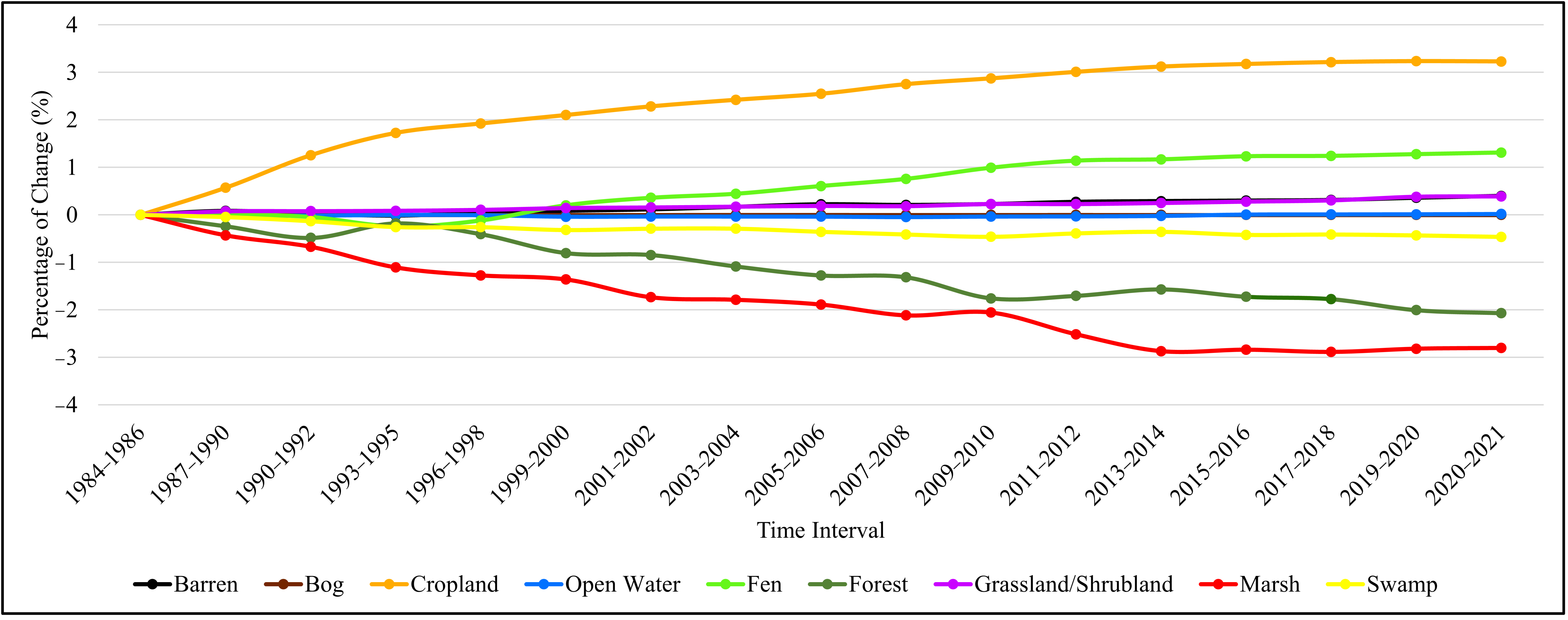
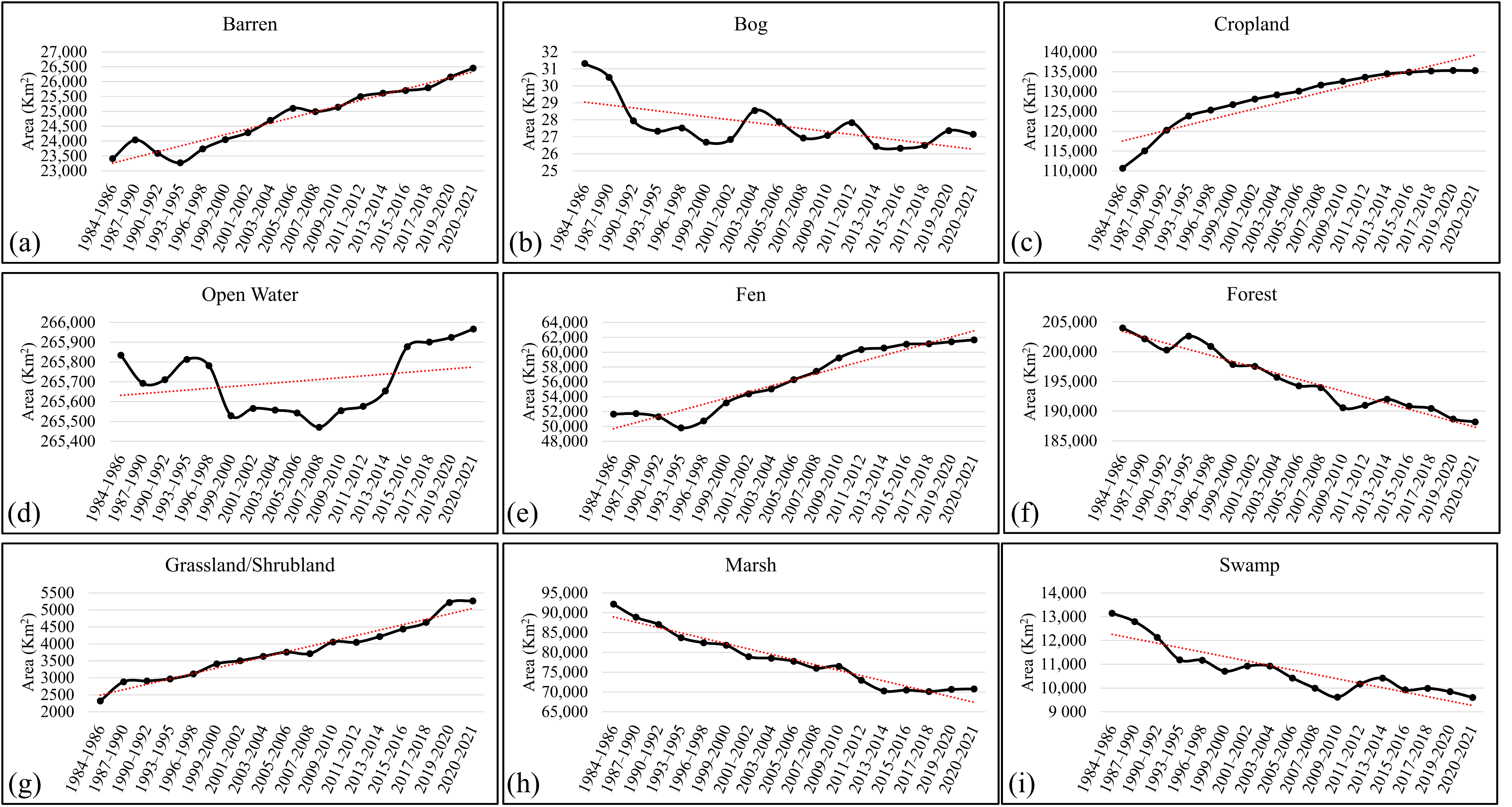
3.2.2. Change Trend Analysis

The computed class areas from the generated wetland maps were examined to quantify the relative changes in the area of each class. To this end, the proportionate area of each class in the earliest time interval was considered as the starting point, and the relative differences were calculated (see Figure 12). The results demonstrated that Open Water and Bog, the majority and minority land covers of the Great Lakes basin, respectively, covered the most consistent amount of area during the study period. Similarly, Barren, Grassland/Shrubland, Fen, and Swamp had relatively stable areas between 1984 and 2021, with slight upward trends for the first three aforementioned classes and a slight downward trend for the last class. The highest increase corresponded to Cropland, with an approximately 3.2% growth in area, indicating the significant impact of anthropogenic practices in this region. In contrast, Marsh and Forest had the two highest downward trends with almost 2.8% and 2.1% losses, respectively, over the past four decades. Overall, the increase and decrease in the areas of Cropland and Forest were expected due to several anthropogenic activities, including agricultural expansion and deforestation, that occurred in the Great Lakes region, especially over recent years.

The areas of each class, derived from the 17 wetland maps, are also presented in Figure 13 to better quantify each class’s dynamic between 1984 and 2021. Figure 13 shows that Open Water, Forest, and Cropland were the most dominant classes in all time intervals, covering areas of approximately 265,500 km², 195,300 km², and 128,300 km², respectively. Regarding wetland classes, the Great Lakes basin was covered mainly by Marsh and Fen, with areas of approximately 78,100 km² and 56,200 km², respectively. Overall, Barren, Cropland, Fen, and Grassland/Shrubland presented steady rising trends with varying slopes, while the Forest, Marsh, and Swamp classes had stable downward trends. For instance, Barren areas started at almost 23,400 km² in the first time interval and increased to more than 26,400 km² in the latest time interval, which is mainly linked to urban growth in metropolitan areas such as Toronto, Buffalo, and Green Bay. Additionally, the Cropland areas exceeded 135,200 km², with an almost 12.2% increase during the study period, and could be considered another human-induced indicator for wetland changes in the study area. Fen experienced a massive increase among wetland classes, almost 10,000 km², reaching an area greater than 61,600 km². Conversely, Marsh experienced the highest rate of decrease, falling from 92,600 km² to 70,700 km². Likewise, the Forest area declined from almost 203,900 km² to approximately 188,100 km² in the past four decades, with anthropogenic activities such as urban and agricultural expansion, as well as misclassification errors in the wetland maps, the likely cause. Moreover, the significant number of forest wildfires recorded in the past few decades could be another contributing factor in the loss of forest area. In particular, the Canadian National Forestry Database and the United States Environmental Protection Agency reported many wildfires events in Ontario, Canada, and Michigan, US, that resulted in notable forest losses [37]. Meanwhile, Open Water and Bog, two classes with minor relative changes (see Figure 12), had fluctuating trends with various downward and upward trajectories, culminating in an increase and a decrease in their area at the end of the study period, respectively.

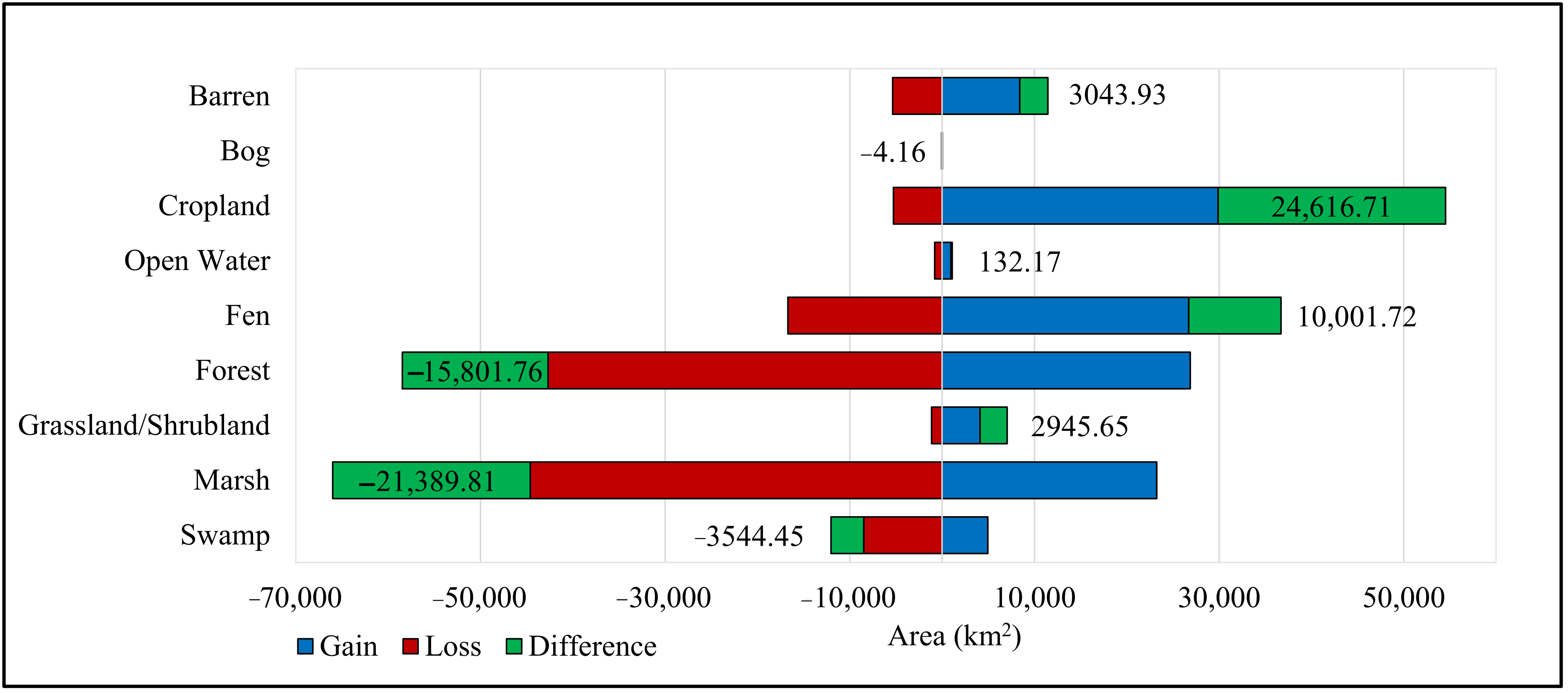
3.2.3. Gain and Loss

The generated binary map of the changed and unchanged areas (Figure 11) was manipulated to illustrate the spatial pattern of wetland gains and losses (Figure 14). The Gain (i.e., wetland gain) is associated with non-wetland classes that were converted to either one of the wetland classes, whereas the Loss (i.e., wetland loss) indicated wetlands that were converted into non-wetland classes. In total, the Great Lakes basin was subjected to 6.8% wetland loss and 4.9% wetland gain between 1984 and 2021. According to the Gain and Loss maps (Figure 14), the Lake Superior subbasin had a higher wetland gain (6.2%) than wetland loss (4.8%) during the past four decades. However, wetland losses exceeded wetland gains in the four other subbasins, with approximate differences of 0.6%, 6.0%, 4.8, and 3.8% for Lake Huron, Lake Ontario, Lake Erie, and Lake Michigan, respectively. Moreover, the loss of coastal Marsh and Swamp were observed in several parts of the Great Lakes basin between 2016 to 2018 (Figure 14), which was in line with the findings of the precious research study [24]. Additionally, coastal wetland loss in some parts of the Great Lakes basin (e.g., Lake Erie and Lake Michigan) were in good agreement with the findings of previous studies [38].

In a detailed quantitative overview, the gain and loss values were also computed for all classes and are illustrated in Figure 15. The Marsh and Forest classes had the two greatest losses of 44,408 km² and 42,406 km², while they also experienced gains of 23,227 km² and 26,866 km², leading a net loss of 21,181 km² and 15,540 km² over the past four decades, respectively. Swamp area also experienced a net decline, losing 8495 km² and gaining only 4950 km², making it the second-largest source of wetland loss in the Great Lakes basin. Meanwhile, Bog, Open Water, and Grassland/Shrubland had the lowest gain and loss values, respectively, which explains the observed relative stability of these classes over the past four decades. Cropland experienced major gains (29,896 km²) and a minor loss (5279 km²), resulting in a net increase of 24,617 km².

Figure 16 and Figure 17 illustrate the wetland gain and loss maps at different time intervals, respectively. According to Figure 16a, the greatest gain in the Great Lakes basin occurred between 1987 and 1995, while the least gain occurred between 2015 and 2021. Lake Superior experienced the most gain between 1990 and 1995, while there was slight gain between 2013 and 2021 (Figure 16b). The most significant gain in Lake Huron happened between 1987 and 1993, whereas the least gain occurred between 2019 and 2021 (Figure 16c). For Lake Ontario, the largest and smallest gains occurred during the 1987–1995 and 2013–2021 intervals, respectively (Figure 16d). The biggest gain in Lake Erie happened between 1987 to 1995, whereas the smallest gain occurred during the 2009–2010 and 2019–2021 intervals, respectively (Figure 16e). Lake Michigan experienced the most gain between 1987 and 1995, while the least gain occurred between 2013 and 2021 (Figure 16f).

According to Figure 17a, the most significant loss in the Great Lakes basin occurred between 1996 and 1998, closely followed by the loss rate between 2013 and 2014. However, the least amount of loss occurred between 2020 and 2021. In Lake Superior, the greatest loss occurred during the 1990–1992 interval, while the smallest loss occurred during the 2019–2021 interval (Figure 17b). It was also observed that most of the Lake Huron’s loss occurred during the 1993–1995 interval, whereas the least loss occurred during the 1996–1998 and 2019–2021 intervals, respectively (Figure 17c). In Lake Ontario, the biggest loss occurred during the 1993–1995 and 2009–2013 intervals, respectively, while the smallest loss occurred during the 1987–1990 and 2015–2018 intervals, respectively (Figure 17d). During the 1987–2000 interval, Lake Erie experienced the greatest loss, whereas the least loss occurred during the 2007–2008 and 2019–2021 intervals, respectively (Figure 17e). The biggest and smallest losses in Lake Michigan occurred during the 1987–2000 and 2019–2021 intervals, respectively (Figure 17f).

3.2.4. Transition between Classes

A From/To map (

Table 4. The land cover transition between each class in the Great Lakes basin between the first (1984–1986) and the last (2020–2021) time intervals.

			2020–2021
		Barren	Bog	Cropland	Open Water	Fen	Forest	Grassland/Shrubland	Marsh	Swamp	Total	Total (%)
	Barren	18,046.3	0.3	3380.1	63.1	208.8	277.8	18.7	1356.0	60.6	23,411.6	3.1
	Bog	0.5	15.0	4.8	0.1	4.5	2.9	0.2	3.1	0.3	31.3	0.0
	Cropland	4624.5	0.2	105,377.8	6.5	73.3	19.6	5.1	543.2	7.5	110,657.8	14.5
1984–1986	Open Water	53.6	0.0	49.2	265,017.9	11.4	17.0	0.1	683.9	1.6	265,834.7	34.8
	Fen	324.1	4.7	3223.3	22.9	34,966.7	6564.6	415.2	5636.8	499.0	51,657.3	6.8
	Forest	673.3	2.9	4718.0	24.6	18,449.4	161,329.6	2432.3	13,333.0	3034.9	203,997.9	26.7
	Grassland/Shrubland	20.9	0.1	326.5	0.1	168.0	288.9	1169.3	319.3	27.5	2320.6	0.3
	Marsh	2496.1	3.7	17,765.7	830.5	6965.9	14,158.4	1077.1	47,550.5	1319.7	92,167.5	12.1
	Swamp	216.4	0.3	429.0	1.1	811.1	5537.4	148.1	1352.0	4652.0	13,147.4	1.7
	Total	26,455.6	27.2	135,274.5	265,966.8	61,659.0	188,196.2	5266.3	70,777.8	9603.0	763,226.2	100.0
	Total (%)	3.5	0.0	17.7	34.8	8.1	24.7	0.7	9.3	1.3	100.0

) was also generated to explore the transition rate between each pair of classes. To this end, the first and the last wetland maps of the Great Lakes basin were compared to determine the amount of land cover transition that occurred between the nine classes. The most significant transition was observed between Forest and Fen, where approximately 18,449 km² of Forest in 1984–1986 was converted to Fen by 2020–2021. Both Open Water and Bog did not experience significant transitions from or to other classes. However, several classes experienced multiple land cover transitions over the past four decades. For example, approximately 17,765 km², 14,158 km², and 6965 km² of Marsh were converted to Cropland, Forest, and Fen during the past four decades, respectively. Among other wetland classes, Fen and Swamp were both primarily transformed into Forest or Marsh. Overall, wetland classes were most commonly converted to Forest or Cropland. The two main land cover origins for an increase in Barren area were found to be Marsh and Cropland, where 2496 km² and 4624 km² of each were converted to Barren, respectively. Furthermore, it was observed that an area of 22,480 km² was converted to Cropland between 1984 and 2021, mainly from Marsh and Forest, highlighting the agricultural expansion occurring in this region.

4. Limitations and Suggestions

In this study, due to the low number and quality of the samples, the Shallow Water class was combined with the Deep Water class to form the Open Water class. However, to conform the five wetland classes specified by the Canadian Wetland Classification System (CWCS, [39]), Bog, Fen, Marsh, Swamp, and Shallow Water, it is suggested additional Shallow Water field samples be collected in order to properly discriminate this class from Deep Water in future studies.

As explained in Section 2.4.2, the CCDC method was used to select the spectrally unchanged samples over the study period. During this process, it was observed that there were a considerable number of samples that had spectrally changed over the past four decades and, thus, were not used in the training and validation of the classification model. This reduced the number of samples for some classes, notably Bog, Grassland/Shrubland, and Swamp, and, consequently, affected the mapping accuracy of these classes. Therefore, similar to the Shallow Water class, it is suggested that more field data be collected and processed for these classes to improve the accuracy of the maps and change detection results. An alternative solution would be using wetland field data collected from other provinces/states of Canada/US with similar landscapes to the Great Lakes region.

The Landsat archive (i.e., Landsat 5, 7, and 8) was employed in this study to map wetlands and assess changes, as it is the only remote sensing system which provides continuous earth observation imagery over the four-decade period. However, Landsat imagery has a spatial resolution of 30 m and, as a result, introduces a source of misclassification in the change analysis. Moreover, discriminating multiple wetland classes using only optical imagery is challenging. For example, SAR data provides additional information to improve the separation of similar classes, such as Swamp and Forest [16,18,40]. Unfortunately, historical SAR data spanning the study period is not available and could not be applied to all classifications. Furthermore, since multiple images were required to produce a cloud-free mosaic image for each time interval (see Table 2), variations between different images could introduce another source of error.

Forest changes may result from clear-cutting or wildfires that mistakenly appeared as changes. It is recommended to further investigate the burned areas and/or clear-cut areas to obtain a more accurate understanding of reasons for change, especially in vegetated areas. To this end, vegetation change detection methods (e.g., [41]) along with our proposed approach would be beneficial.

Wetlands are naturally complex ecosystems that vary between and within individual sites due to changes in vegetation, water, and chemicals related to seasons, weather, and disturbance. The dynamic interaction between wetlands and their surrounding environments could also result in wetland features appearing different between years, although no change has in fact occurred [1].

In summary, there are multiple solutions to improve the accuracy of the results reported in this study. For example, the integration of high-resolution satellite images and accurate elevation information could considerably improve the accuracy of the classification and, subsequently, change the analysis. On the other hand, adding textural and geometrical features to the classification process could help to better separate different wetland types. Moreover, the results of previous studies [23,24,42] showed that integration of multi-temporal SAR and optical images in classification and change detection of wetlands resulted in greater accuracy. The Great Lakes undergo distinct water level variations that affect the water extend [38,43]. Thus, multi-sensor images and InSAR water level and vegetation monitoring datasets could facilitate wetland change analysis [24,43,44]. Finally, using a different channel of SAR images (e.g., X-, C-, and L-band) in InSAR and classification processes could provide constructive information to characterize coastal wetlands in the Great Lakes and, therefore, reduce misclassification [24,43,44,45].

5. Conclusions

Remote sensing has allowed for effective wetland mapping and monitoring applications due to improvements in coverage, accessibility, and processing efficiency. This study utilized the GEE cloud platform and the available Landsat archive to classify wetland and non-wetland classes across the Great Lakes basin over four decades. The resultant classifications achieved an overall accuracy greater than 84% and the change analysis showed that approximately 16% of the study area has undergone landscape change since 1984. The highest increase and decrease in the areas of the classes were observed for Cropland and Forest/Marsh, respectively. Forest mostly transitioned to Fen, Cropland, Marsh, and Swamp, respectively. A notable portion of Marsh was additionally converted into Cropland. These results show that GEE can effectively be applied to monitor wetland change throughout the Great Lakes basin, where continued and improved monitoring will assist in understanding past and present wetland changes for future conservation efforts.

References

1. Mahdavi, S.; Salehi, B.; Granger, J.; Amani, M.; Brisco, B.; Huang, W. Remote sensing for wetland classification: A comprehensive review. GISci. Remote Sens. 2018, 55, 623–658. [Google Scholar] [CrossRef]
2. Fisher, J.; Acreman, M.C. Wetland nutrient removal: A review of the evidence. Hydrol. Earth Syst. Sci. 2004, 8, 673–685. [Google Scholar] [CrossRef] [Green Version]
3. Hey, D.L.; Kostel, J.A.; Crumpton, W.G.; Mitsch, W.J.; Scott, B. The roles and benefits of wetlands in managing reactive nitrogen. J. Soil Water Conserv. 2012, 67, 47A–53A. [Google Scholar] [CrossRef] [Green Version]
4. Kingsford, R.T.; Basset, A.; Jackson, L. Wetlands: Conservation’s poor cousins. Aquat. Conserv. Mar. Freshw. Ecosyst. 2016, 26, 892–916. [Google Scholar] [CrossRef] [Green Version]
5. Amani, M.; Mahdavi, S.; Kakooei, M.; Ghorbanian, A.; Brisco, B.; DeLancey, E.; Toure, S.; Reyes, E.L. Wetland Change Analysis in Alberta, Canada Using Four Decades of Landsat Imagery. IEEE J. Sel. Top. Appl. Earth Obs. Remote Sens. 2021, 14, 10314–10335. [Google Scholar] [CrossRef]
6. Mahdianpari, M.; Jafarzadeh, H.; Granger, J.E.; Mohammadimanesh, F.; Brisco, B.; Salehi, B.; Homayouni, S.; Weng, Q. A large-scale change monitoring of wetlands using time series Landsat imagery on Google Earth Engine: A case study in Newfoundland. GISci. Remote Sens. 2020, 57, 1102–1124. [Google Scholar] [CrossRef]
7. Mahdavi, S.; Salehi, B.; Amani, M.; Granger, J.E.; Brisco, B.; Huang, W.; Hanson, A. Object-based classification of wetlands in Newfoundland and Labrador using multi-temporal PolSAR data. Can. J. Remote Sens. 2017, 43, 432–450. [Google Scholar] [CrossRef]
8. Varin, M.; Theau, J.; Fournier, R.A. Mapping ecosystem services provided by wetlands at multiple spatiotemporal scales: A case study in Quebec, Canada. J. Environ. Manag. 2019, 246, 334–344. [Google Scholar] [CrossRef] [PubMed]
9. Mitsch, W.J.; Gosselink, J.G. The value of wetlands: Importance of scale and landscape setting. Ecol. Econ. 2000, 35, 25–33. [Google Scholar] [CrossRef]
10. Lillo, A.; Matteau, J.-P.; Kokulan, V.; Benalcazar, P. The Contribution of Wetlands Towards a Sustainable Agriculture in Canada; The Canadian Agri-Food Policy Institute: Ottawa, ON, Canada, 2019. [Google Scholar]
11. DeLancey, E.R.; Simms, J.F.; Mahdianpari, M.; Brisco, B.; Mahoney, C.; Kariyeva, J. Comparing Deep Learning and Shallow Learning for Large-Scale Wetland Classification in Alberta, Canada. Remote Sens. 2020, 12, 2. [Google Scholar] [CrossRef] [Green Version]
12. Mahdianpari, M.; Brisco, B.; Granger, J.; Mohammadimanesh, F.; Salehi, B.; Homayouni, S.; Bourgeau-Chavez, L. The Third Generation of Pan-Canadian Wetland Map at 10 m Resolution Using Multisource Earth Observation Data on Cloud Computing Platform. IEEE J. Sel. Top. Appl. Earth Obs. Remote Sens. 2021, 14, 8789–8803. [Google Scholar] [CrossRef]
13. Amani, M.; Salehi, B.; Mahdavi, S.; Granger, J.E.; Brisco, B.; Hanson, A. Wetland Classification Using Multi-Source and Multi-Temporal Optical Remote Sensing Data in Newfoundland and Labrador, Canada. Can. J. Remote Sens. 2017, 43, 360–373. [Google Scholar] [CrossRef]
14. Mohammadimanesh, F.; Salehi, B.; Mahdianpari, M.; Gill, E.; Molinier, M. A new fully convolutional neural network for semantic segmentation of polarimetric SAR imagery in complex land cover ecosystem. ISPRS J. Photogramm. Remote Sens. 2019, 151, 223–236. [Google Scholar] [CrossRef]
15. White, L.; Brisco, B.; Dabboor, M.; Schmitt, A.; Pratt, A. A Collection of SAR Methodologies for Monitoring Wetlands. Remote Sens. 2015, 7, 7615–7645. [Google Scholar] [CrossRef] [Green Version]
16. Brisco, B.; Kapfer, M.; Hirose, T.; Tedford, B.; Liu, J. Evaluation of C-band polarization diversity and polarimetry for wetland mapping. Can. J. Remote Sens. 2011, 37, 82–92. [Google Scholar] [CrossRef]
17. Merchant, M.A.; Warren, R.K.; Edwards, R.; Kenyon, J.K. An Object-Based Assessment of Multi-Wavelength SAR, Optical Imagery and Topographical Datasets for Operational Wetland Mapping in Boreal Yukon, Canada. Can. J. Remote Sens. 2019, 45, 308–332. [Google Scholar] [CrossRef]
18. Brisco, B.; Murnaghan, K.; Wdowinski, S.; Hong, S.-H. Evaluation of RADARSAT-2 Acquisition Modes for Wetland Monitoring Applications. Can. J. Remote Sens. 2015, 41, 431–439. [Google Scholar] [CrossRef]
19. Amani, M.; Salehi, B.; Mahdavi, S.; Brisco, B. Spectral analysis of wetlands using multi-source optical satellite imagery. ISPRS J. Photogramm. Remote Sens. 2018, 144, 119–136. [Google Scholar] [CrossRef]
20. Amani, M.; Ghorbanian, A.; Ahmadi, S.A.; Kakooei, M.; Moghimi, A.; Mirmazloumi, S.M.; Moghaddam, S.H.A.; Mahdavi, S.; Ghahremanloo, M.; Parsian, S.; et al. Google Earth Engine Cloud Computing Platform for Remote Sensing Big Data Applications: A Comprehensive Review. IEEE J. Sel. Top. Appl. Earth Obs. Remote Sens. 2020, 13, 5326–5350. [Google Scholar] [CrossRef]
21. Gorelick, N.; Hancher, M.; Dixon, M.; Ilyushchenko, S.; Thau, D.; Moore, R. Google Earth Engine: Planetary-scale geospatial analysis for everyone. Remote Sens. Environ. 2017, 202, 18–27. [Google Scholar] [CrossRef]
22. Tamiminia, H.; Salehi, B.; Mahdianpari, M.; Quackenbush, L.; Adeli, S.; Brisco, B. Google Earth Engine for geo-big data applications: A meta-analysis and systematic review. ISPRS J. Photogramm. Remote Sens. 2020, 164, 152–170. [Google Scholar] [CrossRef]
23. Valenti, V.L.; Carcelen, E.C.; Lange, K.; Russo, N.J.; Chapman, B. Leveraging Google Earth Engine User Interface for Semiautomated Wetland Classification in the Great Lakes Basin at 10 m With Optical and Radar Geospatial Datasets. IEEE J. Sel. Top. Appl. Earth Obs. Remote Sens. 2020, 13, 6008–6018. [Google Scholar] [CrossRef]
24. Battaglia, M.J.; Banks, S.; Behnamian, A.; Bourgeau-Chavez, L.; Brisco, B.; Corcoran, J.; Chen, Z.; Huberty, B.; Klassen, J.; Knight, J.; et al. Multi-Source EO for Dynamic Wetland Mapping and Monitoring in the Great Lakes Basin. Remote Sens. 2021, 13, 599. [Google Scholar] [CrossRef]
25. Krantzberg, G.; De Boer, C. A valuation of ecological services in the Laurentian Great Lakes Basin with an emphasis on Canada. J. Am. Water Works Assoc. 2008, 100, 100–111. [Google Scholar] [CrossRef]
26. Albert, D.A.; Wilcox, D.A.; Ingram, J.W.; Thompson, T.A. Hydrogeomorphic Classification for Great Lakes Coastal Wetlands. J. Great Lakes Res. 2005, 31, 129–146. [Google Scholar] [CrossRef]
27. Zhu, Z.; Woodcock, C.E. Continuous change detection and classification of land cover using all available Landsat data. Remote Sens. Environ. 2014, 144, 152–171. [Google Scholar] [CrossRef] [Green Version]
28. Foga, S.; Scaramuzza, P.L.; Guo, S.; Zhu, Z.; Dilley, R.D.; Beckmann, T.; Schmidt, G.L.; Dwyer, J.L.; Joseph Hughes, M.; Laue, B. Cloud detection algorithm comparison and validation for operational Landsat data products. Remote Sens. Environ. 2017, 194, 379–390. [Google Scholar] [CrossRef] [Green Version]
29. USGS. United States Geological Survey (USGS) Landsat Collection 1 Level-1 Quality Assessment Band; USGS: Reston, VA, USA. Available online: https://www.usgs.gov/landsat-missions/landsat-collection-1-level-1-quality-assessment-band (accessed on 20 April 2022).
30. Ghorbanian, A.; Kakooei, M.; Amani, M.; Mahdavi, S.; Mohammadzadeh, A.; Hasanlou, M. Improved land cover map of Iran using Sentinel imagery within Google Earth Engine and a novel automatic workflow for land cover classification using migrated training samples. ISPRS J. Photogramm. Remote Sens. 2020, 167, 276–288. [Google Scholar] [CrossRef]
31. Mohammadi Asiyabi, R.; Sahebi, M.R.; Ghorbanian, A. Segment-based bag of visual words model for urban land cover mapping using polarimetric SAR data. Adv. Space Res. 2021, in press. [Google Scholar] [CrossRef]
32. Achanta, R.; Susstrunk, S. Superpixels and polygons using simple non-iterative clustering. In Proceedings of the IEEE Conference on Computer Vision and Pattern Recognition, Honolulu, HI, USA, 21–26 July 2017; pp. 4651–4660. [Google Scholar]
33. Ghorbanian, A.; Zaghian, S.; Asiyabi, R.M.; Amani, M.; Mohammadzadeh, A.; Jamali, S. Mangrove Ecosystem Mapping Using Sentinel-1 and Sentinel-2 Satellite Images and Random Forest Algorithm in Google Earth Engine. Remote Sens. 2021, 13, 2565. [Google Scholar] [CrossRef]
34. Amani, M.; Brisco, B.; Afshar, M.; Mirmazloumi, S.M.; Mahdavi, S.; Mirzadeh, S.M.J.; Huang, W.; Granger, J. A generalized supervised classification scheme to produce provincial wetland inventory maps: An application of Google Earth Engine for big geo data processing. Big Earth Data 2019, 3, 378–394. [Google Scholar] [CrossRef]
35. Amani, M.; Mahdavi, S.; Afshar, M.; Brisco, B.; Huang, W.; Mohammad Javad Mirzadeh, S.; White, L.; Banks, S.; Montgomery, J.; Hopkinson, C. Canadian wetland inventory using google earth engine: The first map and preliminary results. Remote Sens. 2019, 11, 842. [Google Scholar] [CrossRef] [Green Version]
36. Amani, M.; Brisco, B.; Mahdavi, S.; Ghorbanian, A.; Moghimi, A.; Delancey, E.; Merchant, M.A.; Jahncke, R.; Fedorchuk, L.; Mui, A. Evaluation of the Landsat-based Canadian Wetland Inventory Map using Multiple Sources: Challenges of Large-scale Wetland Classification using Remote Sensing. IEEE J. Sel. Top. Appl. Earth Obs. Remote Sens. 2020, 14, 32–52. [Google Scholar] [CrossRef]
37. National Forestry Database. Forest Area Burned and Number of Forest Fires. Available online: http://nfdp.ccfm.org/en/data/fires.php (accessed on 28 February 2022).
38. Uzarski, D.G.; Brady, V.J.; Cooper, M.J.; Wilcox, D.A.; Albert, D.A.; Axler, R.P.; Bostwick, P.; Brown, T.N.; Ciborowski, J.J.H.; Danz, N.P.; et al. Standardized Measures of Coastal Wetland Condition: Implementation at a Laurentian Great Lakes Basin-Wide Scale. Wetlands 2017, 37, 15–32. [Google Scholar] [CrossRef] [Green Version]
39. National Wetlands Working Group. The Canadian Wetland Classification System; Lands Conservation Branch, Canadian Wildlife Service, Environment Canada: Toronto, ON, Candada, 1997. [Google Scholar]
40. Amani, M.; Salehi, B.; Mahdavi, S.; Brisco, B. Separability analysis of wetlands in Canada using multi-source SAR data. GISci. Remote Sens. 2019, 56, 1233–1260. [Google Scholar] [CrossRef]
41. Mohsenifar, A.; Mohammadzadeh, A.; Moghimi, A.; Salehi, B. A novel unsupervised forest change detection method based on the integration of a multiresolution singular value decomposition fusion and an edge-aware Markov Random Field algorithm. Int. J. Remote Sens. 2021, 42, 9376–9404. [Google Scholar] [CrossRef]
42. Bourgeau-Chavez, L.L.; Riordan, K.; Miller, N.; Nowels, M.; Powell, R. Remotely Monitoring Great Lakes Coastal Wetlands with Multi-Sensor, Multi-Temporal SAR and Multi-Spectral Data. In Proceedings of the IGARSS 2008—2008 IEEE International Geoscience and Remote Sensing Symposium, Boston, MA, USA, 7–11 July 2008; pp. I-428–I-429. [Google Scholar]
43. Wilcox, D.A.; Thompson, T.A.; Booth, R.K.; Nicholas, J.R. Lake-Level Variability and Water Availability in the Great Lakes; U.S. Geological Survey: Reston, VA, USA, 2007. [Google Scholar]
44. Chen, Z.; White, L.; Banks, S.; Behnamian, A.; Montpetit, B.; Pasher, J.; Duffe, J.; Bernard, D. Characterizing marsh wetlands in the Great Lakes Basin with C-band InSAR observations. Remote Sens. Environ. 2020, 242, 111750. [Google Scholar] [CrossRef]
45. Chen, Z.; Banks, S.; Behnamian, A.; White, L.; Montpetit, B.; Pasher, J.; Duffe, J. Characterizing the Great Lakes Coastal Wetlands with InSAR Observations from X-, C-, and L-Band Sensors. Can. J. Remote Sens. 2020, 46, 765–783. [Google Scholar] [CrossRef]
Figure 1. The study area (the Great Lakes basin and five subbasins of Lake Superior, Lake Huron, Lake Ontario, Lake Erie, and Lake Michigan) and the distribution of field data. The red box shows the location of the study area.
Remotesensing 14 03778 g001
Figure 2. An example of the conversion of (a) point-based field samples to (b) polygon samples. The red color shows the boundary of a Fen area.
Remotesensing 14 03778 g002
Figure 3. The Continuous Change Detection and Classification (CCDC) algorithm for selecting spectrally unchanged field samples over the past four decades from the study area (NDVI: Normalized Difference Vegetation Index, NDWI: Normalized Difference Water Index, NDBI: Normalized Difference Build-up Index).
Remotesensing 14 03778 g003
Figure 4. Classification method to produce wetland maps in the Great Lakes.
Remotesensing 14 03778 g004
Figure 5. The method for wetland Change Detection (CD) between two time intervals, where T indicates the time interval (see Table 2).
Remotesensing 14 03778 g005
Figure 6. The method for wetland Change Detection (CD) over the entire four decades. T indicates the time interval (see Table 2) and CD is the method proposed in Figure 5.
Remotesensing 14 03778 g006
Figure 7. Generated wetland map of the (a) Great Lakes and (bf) its subbasins (i.e., Lake Superior, Lake Huron, Lake Ontario, Lake Erie, and Lake Michigan, respectively) using satellite imagery between 2020 and 2021 as the reference time interval.
Remotesensing 14 03778 g007
Figure 8. Generated wetland map of the Great Lakes basin using satellite imagery between 2020 and 2021 along with (a,b) two zoomed areas (wetland map and high-resolution satellite imagery) to illustrate the visual accuracy of the resultant classification.
Remotesensing 14 03778 g008
Figure 9. Overall Accuracy (OA), Kappa Coefficient (KC), and F Score values of 17 wetland maps of the Great Lakes basin between 1984 and 2021.
Remotesensing 14 03778 g009
Figure 10. (a) User Accuracies (UAs) and (b) Producer Accuracies (PAs) of nine classes of the generated wetland maps for all time intervals between 1984 and 2021.
Remotesensing 14 03778 g010
Figure 11. The produced changed and unchanged binary map of the (a) Great Lakes and (bf) its subbasins (i.e., Lake Superior, Lake Huron, Lake Ontario, Lake Erie, and Lake Michigan, respectively) between 1984 and 2021.
Remotesensing 14 03778 g011
Figure 12. Trends of the relative area change for various classes in the Great Lakes basin extracted from the corresponding wetland maps from 1984 and 2021.
Remotesensing 14 03778 g012
Figure 13. Variation of the areas of the classes in the Great Lakes basin extracted from the corresponding wetland maps from 1984 and 2021. (ai) respectively provide the results for the Barren, Bog, Cropland, Open Water, Fen, Forest, Grassland/Shrubland, Marsh, and Swamp classes. The black and red lines indicate the line chart and linear regression trendline, respectively.
Remotesensing 14 03778 g013
Figure 14. Gain and Loss map of wetlands of the (a) Great Lakes basin and (bf) its subbasins (i.e., Lake Superior, Lake Huron, Lake Ontario, Lake Erie, and Lake Michigan, respectively) in the past four decades.
Remotesensing 14 03778 g014
Figure 15. Gain, Loss, and their differences for each class in the Great Lakes basin over the past four decades. The difference values are illustrated by black numbers.
Remotesensing 14 03778 g015
Figure 16. Wetland gain maps of the (a) Great Lakes basin and (bf) its subbasins (i.e., Lake Superior, Lake Huron, Lake Ontario, Lake Erie, and Lake Michigan, respectively) at different time intervals.
Remotesensing 14 03778 g016
Figure 17. Wetland loss maps of the (a) Great Lakes basin and (bf) its subbasins (i.e., Lake Superior, Lake Huron, Lake Ontario, Lake Erie, and Lake Michigan, respectively) at different time intervals.
Remotesensing 14 03778 g017