Article

End-to-End Prediction of Lightning Events from Geostationary Satellite Images

1
Institute of Computer Science, Johannes Gutenberg University Mainz, 55128 Mainz, Germany
2
German Weather Service, 63067 Offenbach, Germany
3
Institute for Atmospheric Physics, Johannes Gutenberg University Mainz, 55128 Mainz, Germany
*
Author to whom correspondence should be addressed.
Remote Sens. 2022, 14(15), 3760; https://doi.org/10.3390/rs14153760
Submission received: 15 June 2022 / Revised: 30 July 2022 / Accepted: 2 August 2022 / Published: 5 August 2022
(This article belongs to the Special Issue Artificial Intelligence for Weather and Climate)

Abstract

:
While thunderstorms can pose severe risks to property and life, forecasting remains challenging, even at short lead times, as these often arise in meta-stable atmospheric conditions. In this paper, we examine the question of how well we could perform short-term (up to 180 min) forecasts using exclusively multi-spectral satellite images and past lighting events as data. We employ representation learning based on deep convolutional neural networks in an “end-to-end” fashion. Here, a crucial problem is handling the imbalance of the positive and negative classes appropriately in order to be able to obtain predictive results (which is not addressed by many previous machine-learning-based approaches). The resulting network outperforms previous methods based on physically based features and optical flow methods (similar to operational prediction models) and generalizes across different years. A closer examination of the classifier performance over time and under masking of input data indicates that the learned model actually draws most information from structures in the visible spectrum, with infrared imaging sustaining some classification performance during the night.

1. Introduction

Thunder and lightning are violent atmospheric events that must have impressed humans since prehistoric times. Lightning itself, as well as strong winds and precipitation, hail, or even down bursts or tornadoes that might accompany thunderstorms, are not only impressive appearances in satellite images but can pose significant risk to life and property. Even in modern times, fatalities and severe damages from thunderstorms are still occurring at unfortunate rates, and many commercial operations, such as airports or public outdoor events (sports, music, gatherings), rely on risks assessments and prediction of lightning in order to operate safely. In this context, accurate forecasts for the next few hours are particularly important. Usually, thunderstorms are associated with lightning, which easily can be detected by triangulation using multiple radio wave antennas.
Unfortunately, the prediction of thunderstorms and lightning (Cb) is a very difficult problem: The development of atmosphere’s electric field with locally strong charges of different signs is crucially dependent on cloud processes. Charge generation is based on the collision of ice particles (ice crystals, graupel or hail particle) in the presence of super-cooled water droplets [1]. Furthermore, other processes of this kind are proposed for charge generation; see, e.g., [2]. Nevertheless, the collisions are enhanced in strong, localized atmospheric updrafts that are typically formed by frontal movements or spontaneous convective events induced by heat in situations of unstable atmospheric layering. In particular, the latter effects are highly sensitive to small-scale perturbations and thus are hard to predict.
Although significant improvements in Cb forecasting have been achieved with numerical weather prediction (NWP) [3,4], accurate forecasts of Cb location and strength are still a major challenge. Hence, nowcasting methods are typically used to issue warnings with short lead times (in the range of up to a few hours) [5]. An early overview of nowcasting of (severe) weather phenomena is given in [6]. Nowcasting can in general be viewed as a special type of video prediction problem, that is, classification or regression based on a temporal sequence of images. Thus, methods proposed for, e.g., video frame prediction in natural videos are applicable to nowcasting and are related; see [7].
Radar-based methods are often used for regional nowcasting—in particular, the (Doppler-) radar-based remote sensing of (heavy) precipitation events and their movement, depending on the method in combination with lightning data [8]. The forecast is typically based on two subsequent images and extrapolation of the movement of the observed storm cells, e.g., by optical flow methods [9] or tracking methods [10]. This limits the ability to predict newly forming or decaying cells and limits long-term precision. For example, operational systems such as NowCastMIX [10] struggle with predictions for lead times beyond two hours. That is why for longer lead times, NWP models are used.
An alternative source of information are images recorded by geostationary satellites. They cover larger regions than methods based on weather radar. For example, the SEVIRI instrument onboard Meteosat’s second generation (MSG) platform provides data in twelve spectral bands with a temporal resolution of 15 min and a spatial resolution with 3   k m × 3   k m sub satellite point, which corresponds to 0.05 ° × 0.03 ° in Central Europe. These data can be used like radar data to determine atmospheric motion vectors (AMVs) using optical flow and to provide information about the brightness temperature of clouds (BT), which can be used to indicate thunderstorms. For example, the physically motivated usage of the “sandwich” method, which is based on the BT difference between the 6.3 water vapor (WV) channel and the IR window channel [11], or alternatively the 7.3 WV channel [12]. Yet, Cbs are defined by lightning. Hence, in order to improve the accuracy of the detection of Cbs, which is the basis for the nowcasting, it is recommended to use lightning data in addition. For example, [13] use the Advanced Baseline Imager (ABI) and flash-extent density (FED) from the Geostationary Lightning Mapper (GLM) on board GOES-16, as well as satellite and solar zenith angles and geo-coordinates to predict “intense convection”. In [14], satellite-based information is combined with lightning data from the Vaisala Global Lightning Detection Network (GLD360) and information from NWP. Moreover, a combination of satellite and radar information is applied; for example, [15] make use of five temporal images from two ABI channels to predict convective regions, derived from Multi-Radar Multi-Sensor (MRMS) precipitation types.
However, it remains unclear whether physical nowcasting methods are capable of making the best possible use of the available information given in the satellite image and lightning data. As discussed before, current approaches, e.g., [14,16,17], do not take into account the decay or development of (new) cells. Corresponding information may be hidden in the input data and unused. The visual analysis of thunderstorms based on lightning data and satellite imagery suggests that there may be more information in the data that can be extracted. Thus, an obvious alternative is to resort to machine learning [18,19] and in particular deep representation learning techniques [13,20], which have, in recent years, become able to automatically build highly predictive statistical models even from data with extremely complex statistical dependency structure, such as differentiating different breeds of dogs in general photography [21,22,23].
Our study follows this approach: We predict lighting events from image sequences containing satellite imagery and a map of recent lightning events through an image-to-image translation performed by (a variant of) a convolutional U-Net [24], which could be considered a “canonical” network approach to image-segmentation and translation tasks. Our study is designed in particular to address the question of what insight can be gained from satellite images alone for short-term Cb-forecasting, and which parts of the data are most important to this end. The use of machine learning methods, and specifically deep neural networks, has been studied previously in the literature [25,26,27,28,29]. Specifically, U-Nets have been used in related studies for precipitation forecasting [30,31]. Regarding convection, [32] published a study that uses radar images (2 min, 1 km grid) to predict precipitation with a lead time up to 6 h using a (residual) U-Net. Similarly, Shi et al. [33] train a Trajectory GRU model to predict precipitation based on radar images (6 min, ca. 1 km grid). A random forest classifier to detect convective initiation (CI) from geostationary satellite data training on hand-crafted features, where CI is derived from radar data, was proposed in [34]. A similar model based on four commonly available surface weather variables (air pressure at station level (QFE), air temperature, relative humidity, and wind speed) to predict lightning events for lead times with up to 30 min training a decision tree was developed in [35].
However, lighting prediction comes with the problem of heavy class imbalance which is a general challenge for classification with statistical machine learning: In many relevant scenarios, lighting events are rather rare; thus, a classifier that just predicts “no (nearby) lightning” for all outputs can easily reach accuracies close to 100 % . Previous work has mitigated this issue by resampling in evenly balanced examples [18] or considering conditions with high prevalence [20], which then also assumes balanced base-rates when making predictions. In our paper, we develop a method to automatically balance class weights to optimize a deep learning classifier for high predictive power (such as high critical success index, CSI). This permits a simple “end-to-end” training with operationally meaningful predictions (i.e., using recent lightning and satellite observations, the classifier predicts future events with above-chance accuracy). To obtain an indicator of the quality achieved, our results are compared with those of an optical flow-based nowcasting method of the German Weather Service (DWD).
A second and possibly even more interesting question is understanding which information actually contributes to making better predictions. Having a strong classifier that outperforms hand-engineered operational models by simple, automatic statistical learning opens up the opportunity to study this question: By withholding data at the learning stage and tracking the reduction in performance, we can attribute how much information the classifier was able to draw from these sources (formally as lower bound of how much statistical information about the event is contained in portions of the data). We conduct an experiment where we measure the variability of the prediction performance over different times of the day, and retrain classifiers for visible (including a 1.6 μ m near-infrared channel), infrared, and two water vapor bands.
Overall, our study makes two key contributions: (i) a simple method for end-to-end training of lightning events from image data that is both practical (applicable to data with real-world, skewed prior class frequencies) and accurate (outperforming state-of-the-art optical flow-based systems), and (ii) we obtain some novel insights of which sources of information are useful for making predictions by examining the performance characteristics of the learned classifier.

2. Materials and Methods

Our method performs statistical learning to learn a mapping that takes satellite images and measurements of recent lightning activity as input and predicts future lighting activity as output, with a specific lead time.
Satellite images: Formally, we define the geostationary satellite images as functions
S : R × [ 79 , 79 ] × [ 81 , 81 ] × R R ,
denoted as S t ( θ , ϕ , λ ) , where t is the time at which the image capturing has begun, θ and ϕ are the longitude and latitude, respectively, and λ refers to the wave-length band measured. The specific satellite imagery used is provided via the Spinning Enhanced Visible and InfraRed Imager (SEVIRI) of the Meteosat Second Generation (MSG) system, and obtained from EUMETSAT [36]. Images are available in 12 discrete frequency bands with a finite temporal resolution of t s = 15 min. Eight bands represent the thermal infrared (IR) range, providing radiance resulting from the emission of the atmosphere and the Earth surface. They can by used to estimate the brightness temperature of the atmosphere and the surface. Three channels in the visible (VIS) spectrum measure the reflection of solar light at clouds or the Earth’s surface. This information can be used to retrieve the albedo of clouds and the surface. Lastly, the High-Resolution Visible (HRV) channel contains multiple broadband detection elements to scan the Earth with a lower sampling distance. The spatial resolution of the satellite images in Central Europe is roughly 0.05 ° latitude and 0.03 ° longitude (except the HRV band, which we do not consider). All satellite data are projected to an equirectangular projection with an equal spatial resolution of 0.05 ° . We represent the satellite data as collections of 2D images S λ , t as data with values quantized to a 16-bit integer. 
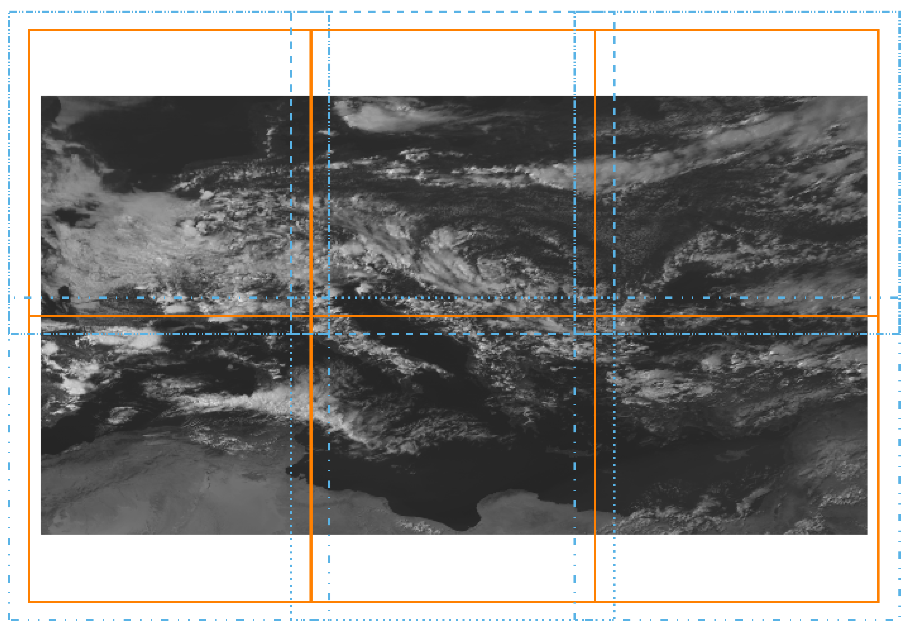
Figure 1b–d show examples of processed satellite imagery of the VIS006 ( λ = 0.6   μ m), WV062 ( λ = 6.2   μ m), and IR120 ( λ = 12   μ m) channels at 4 June 2016 at 12:00 h UTC, where a lot of lightning occurred across Central Europe. The images already indicate that the optical band might be more informative, as the infrared channels only see the cloud tops. However, the patterns in the visible spectrum are complex and not easy to capture in a hand-designed classifier.
Lightning images: Measurements of lightning activity are given as point sets { l 1 , , l n l } R 4 , with two spatial geo-coordinates, a time coordinate, and the electrical current I i . The lightning data used in this study were obtained from the LINET lightning detection network [8]. LINET is a low-frequency long-range lightning detection network (VLF/LF) using the time-of-arrival (TOA) method, consisting of several ground-based lightning sensors. For further processing, we convert the point set into images, with the same spatial and temporal resolution of the satellite images. To this end, we bin all lightning events in an aggregation time span of t a = 15 min, during which the satellite data have been measured, or, during experiments with varying lead-time Δ t , offset by the corresponding Δ t , and binarize them by setting the closest pixel to 1 (with background set to 0). To filter out potential noise, only lightning events with an electric current of at least 1 kA were considered. We denote the resulting lightning images by L t . Figure 1a shows an example of a processed lightning image for the same example date (4 June 2016, 12 h UTC).
The region of interest (ROI) in our work is the mid-latitudes in Central Europe, between 2.0 ° W and 21.5 ° E , and 44.5 ° N and 57.5 ° N . The data are cropped to the defined ROI and split up in smaller patches, according to Appendix A.3. We focus our work on the months May to August in the years of 2016 and 2017. As additional test data set, we use data from August and September of 2021. Detailed information about the data and their use can be seen in Table A1 and Table A2 for 2016/2017 and 2021, respectively. The processing of the data is done using multiple tools, such as pyPublicDecompWT [37], SatPy [38], Pyresample [39], and Cartopy [40].
The learning task can now be posed as a probabilistic prediction of a future lightning image: Let t 0 denote the current time, Δ t the lead time for the prediction, t s the temporal sample spacing, t a the aggregation time span (in our case: t s = t a = 15 min ) , and k the number of past satellite images used for the prediction. With this information, we want to determine a probabilistic classifier f θ that computes a probability map that specifies for each pixel the likelihood of a lightning event being marked in the future lightning image:
f θ L t 0 , S t 0 , L t 0 1 · t s , S t 0 1 · t s , , L t 0 k · t s , S t 0 k · t s L t 0 + Δ t .
This problem is solved by representing the function f θ by a deep neural network with parameters θ R d . Learning is performed using maximum-likelihood: We assume that we are given a set of N training images with pixel-dimensions ( W , H ) and determine a good-fitting θ ^ as a (local) maximum of the likelihood function with L1 regularization:
θ ^ = arg max θ R d λ R d j = 1 d | θ j | + i { 1 , , N } x { 1 , , W } y { 1 , , H } w f θ ( i ) , L t 0 + Δ t ( i ) , r s [ x , y ] · f θ ( i ) , L t 0 + Δ t ( i ) [ x , y ] ,
with
f θ ( i ) , L t 0 + Δ t ( i ) = log f θ ( i ) · L t 0 + Δ t ( i ) positives + log 1 f θ ( i ) · 1 L t 0 + Δ t ( i ) negatives ,
f θ ( i ) = f θ L t 0 ( i ) , S t 0 ( i ) , L t 0 1 · t s ( i ) , S t 0 1 · t s ( i ) , , L t 0 k · t s ( i ) , S t 0 k · t s ( i ) .
Here, the operator [ x , y ] refers to the pixel at position x , y in the respective images; and w denotes a per-pixel class weight, based on the prediction skill of the sample. L1 regularization is scaled by the factor λ R .
The main issue with the cross entropy (CE)-based loss function shown in Equation (4) is the naive (unweighted) summation over all pixels, regardless of their classification. Even when including all pixels in a search radius  r s , the amount of pixels “with lightning” is extremely sparse. Therefore, we add the event-based, per-pixel weight w in Equation (3), which addresses the issue of heavy class imbalance in a sample. This differs from per-sample weighting strategies based on class balance, such as [41]. Per-sample weights work well with known class imbalances, e.g., when data from one class are underrepresented in the data set, by scaling the importance of single samples. This is only partially useful in our case: Thunderstorms are comparatively rare, but when they occur, lightning activity is reasonably high, spanning over multiple pixels in a sample.
In the following, we will construct a per-pixel weight map w, based on the samples class labels L t 0 + Δ t ( i ) , the predictions f θ ( i ) , and a (fixed) “search radius” ( r s ) as follows:
w f θ ( i ) , L t 0 + Δ t ( i ) , r s [ x , y ] = ω lightning , if L t 0 + Δ t ( i ) [ x , y ] = 1 or ( x , y ) FP r s f θ ( i ) , L t 0 + Δ t ( i ) ω no - lightning , otherwise ,
where FP r s ( p , l ) is the set of pixels classified as false positive given the search radius r s , the predictions p, and ground truth labels l of the sample, and ω lightning is the modified class-weight of the “lightning” class in the data set, and ω no - lightning its corresponding counterpart. The class-weight ω cw of a class “cw” is defined as
ω cw = 1 2 × 1 | cw | ,
where | cw | is the amount of instances of the class. Scaling by 1 2 keeps the overall loss at a similar magnitude, so that the sum of the weights of all examples roughly stays constant. The values of ω lightning and ω no - lightning are pre-computed for the whole training split of the data set, and are shown in Table 1. Taking false positives into account, w will adapt to the performance of the classifier f. The training split of the data set is detailed in Table A1.
Table 1. Computed pixel-weights of the training split for the 2016/2017 data set, based on class-weights shown in Table 2 and Equation (7).
ClassPixel-Weight
ω lightning 3.33
ω no - lightning 5 × 10⁻⁵
The search radius  r s is used to model the label uncertainty introduced by various factors, such as the dislocation between lightning and the fictitious center of the Cb, the geolocation error of the satellite, and the movement of the cloud [12]. During the computation of w, it is used to determine false positive predictions. The weight map w can efficiently be computed at every training step in parallel. During training, the loss values are averaged over all pixels and samples in a batch.
The network f used in our study is based on the U-Net [24] architecture, combined with ResNet-v2 [42] residual blocks, adapted to work with three-dimensional input.
The input to our model is of the form ( B , H , W , T , C ) , where B is the batch size, H and W the height and width of an image, T the amount of time-frames, and C the amount of channels. We fixed the height and width of our model to be 256 px × 256 px, which equals 12.8° × 12.8°, or roughly 1425 km × 1425 km. Larger input areas are split up according to the domain decomposition scheme described in Appendix A.3. Further, each input possesses a boundary region, overlapping with neighboring inputs, which allows for a more precise prediction of the non-overlapping region, but which is excluded from the optimization process and evaluation.
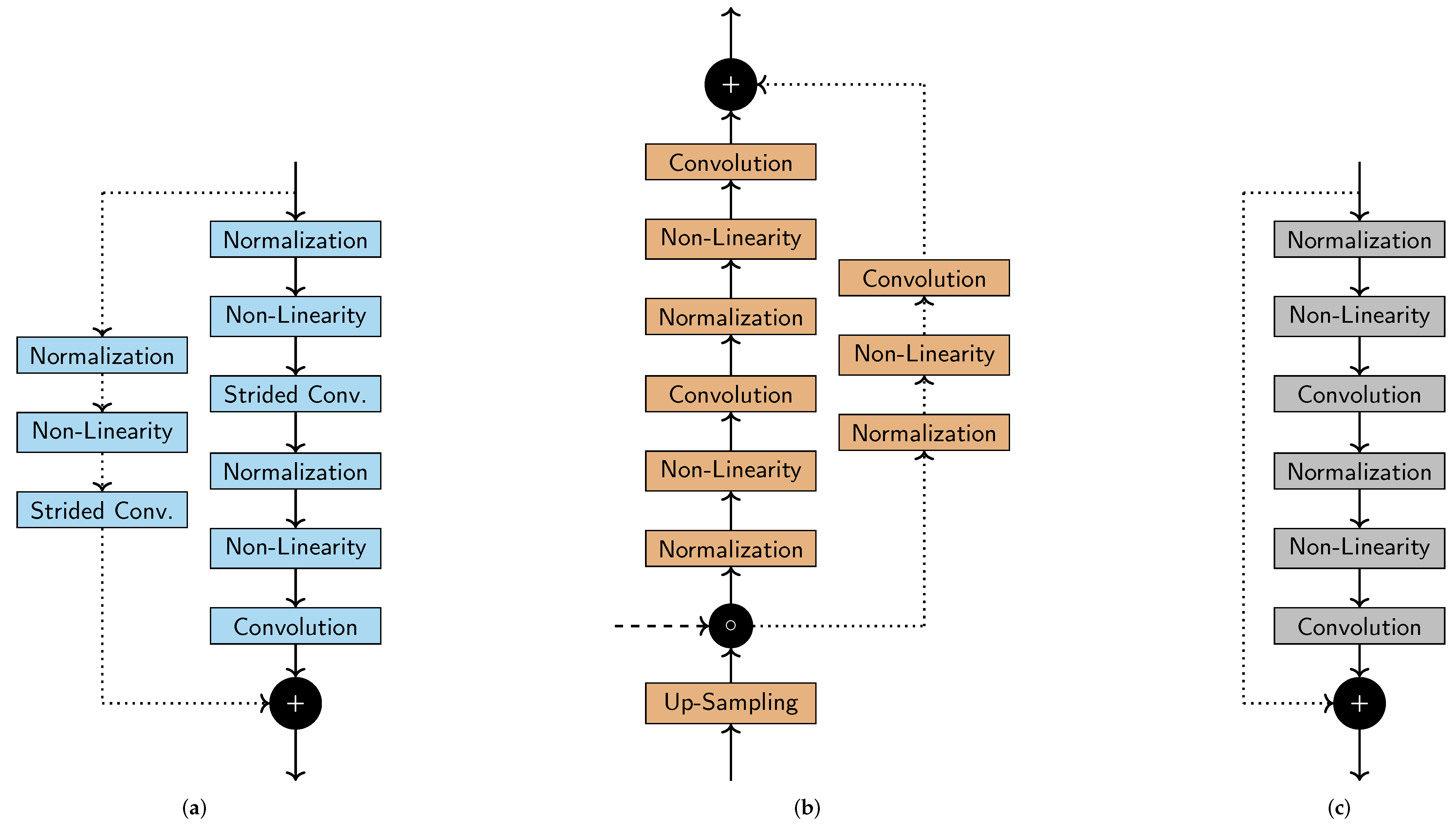
Figure 2 shows an overall view of the used network architecture. The U-Net structure, including skip-connections, can be seen. Varying from the original architecture, we replace the stacked convolution layers and the pooling layer at each down/up sampling step with residual blocks (with stride where necessary). Instead of cropping the feature map of the contracting path, we use the feature map after the down-sampling operator. We use convolutions for down-sampling, but deterministic trilinear up-sampling operations. Deviating from the original architecture, we replace batch normalization layers with instance normalization [43], which normalizes each element of the batch independently, i.e., only across the spatial and time dimension.
The residual blocks consist of full pre-activation units, optionally paired with pre-activated convolution shortcuts, as described in [23]. Figure 3 illustrates the used residual (Figure 3c), down-sampling (Figure 3a), and up-sampling blocks (Figure 3b). Convolution layers use 3 × 3 × 3 filters for up- and down-sampling, and 1 × 1 × 1 otherwise. Non-linear layers consist of ReLU [44] activation functions.
As usual, we increase the amount of channels per block (representing coarser spatial scales). Empirically, we found good validation results for a stronger increase (only) for larger lead-times—details are shown in Table 3. When growing, it follows an exponential curve countering the spatial down- and up-sampling per block in the U-Net, which restraints memory use for weights and activations. The resulting network can be trained on consumer graphics cards at a reasonable batch sizes. Together with the training settings, the expressivity of the neural network is adapted to “match” the complexity of the modeled problem.
Our model is trained using stochastic gradient descent (SGD) with momentum [45] using decoupled weight decay (SGDW) [46] to optimize the loss function, described in Equation (3). The base learning rate (LR) is set as λ = 0.5 , and the weight decay (WD) and L1 regularization are set based on the number of channels of the network, as shown in 
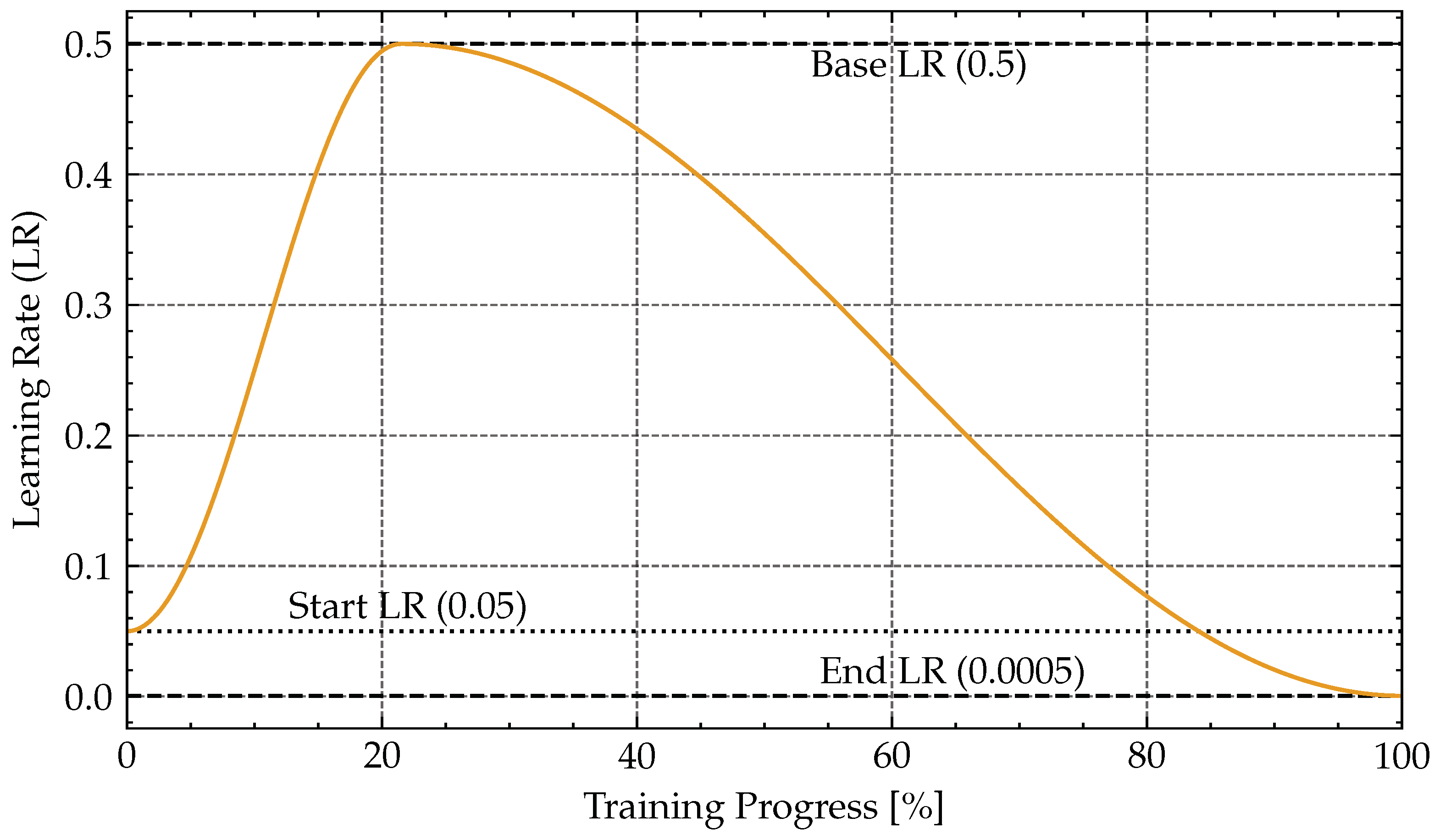
Table 4. We use a batch size of 64 and train the network for 14 epochs. In each epoch, the network trains on a random permutation of the complete training data set. At the end of each epoch, we validate the network’s performance on the validation data set and save its parameters to disk. Every 8th batch, we adapt the decision threshold based on the current best performance. During training, the LR is scheduled with a 1-cycle LR scheduler [47] (two-phase, cosine decay). The learning rate schedule throughout the training process is discussed in more detail in Appendix A.5 and is depicted in Figure A2. Additional to the use of our custom weighted loss function, samples with no lightning activity are discarded during training.
All parameters (of all experiments) were tuned based on data given in Table A1. Our method uses the following input features: SEVIRI channel VIS 0.6, VIS 0.8, nIR 1.6, IR 3.9, WV 6.2, WV 7.3, IR 8.7, IR 9.7, IR 10.8, IR 12.0, IR 13.4 and the most recent lightning events from LINET.
We use PyTorch [48] for all of our experiments and train on a single machine, equipped with an Intel Core i7-8700 Processor and a single NVIDIA TITAN RTX GPU. A reference implementation is provided under a free license.

3. Results

We evaluate our method on the testing data set aside from the original 2016/17 data set (Table A1 in the Appendix A.1), as well as testing data from the month of August and September of 2021, for which comparison data with a nowcasting method [14] at DWD were available. In line with good experimental practice, all hyperparameter tuning has been concluded using validation data before running any inference on any test data has been performed (with frozen, final hyperparameter settings). In particular in our case, where substantial hyperparameter tuning was required, this protocol minimizes the risk of reporting a coincidental success. Further, training and testing were performed 5 times with independent random initialization and training of the network, which can always lead to (a bit of) spread in the results, and mean and standard deviation are reported.
We report the critical success index (CSI) (see Appendix A.2 for details) of the deep network and a base-line “persistence” method, which just assumes that the most recent lightning events at the start of the prediction period persist at the same spot indefinitely. We also compute an “improvement factor” that measures the factor by which the deep network outperforms the base-line persistence model in terms of CSI. As discussed in more detail in Appendix A.4, this makes it easier to compare to other methods while avoiding misjudgement due to small deviations in the evaluation protocols for the corresponding CSIs.
The findings are shown in Figure 4 and Table 5.

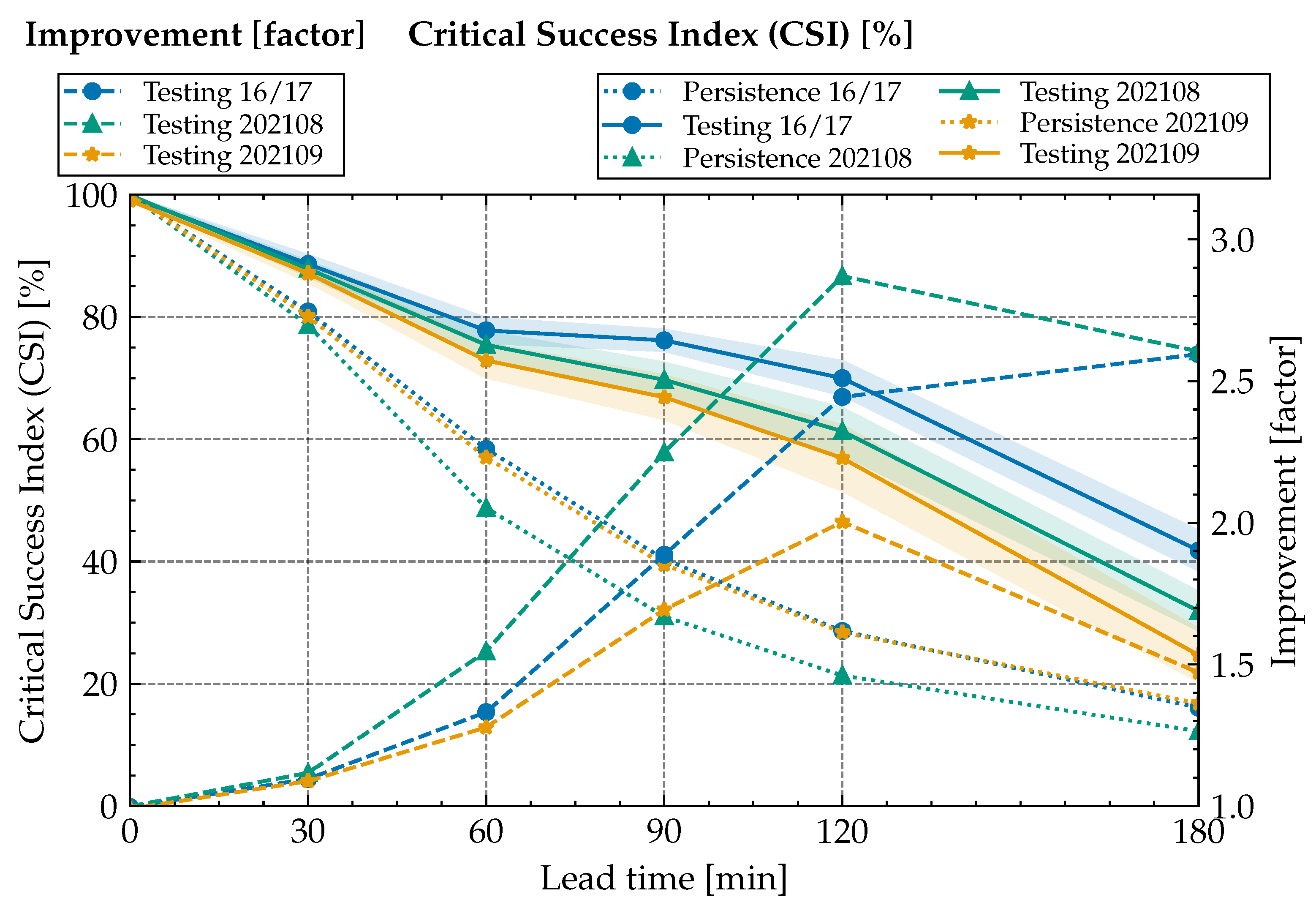
3.1. Classifier Performance and Base-Line Comparison

As a first sanity check, for zero lead time, the network reaches very close to 100 % success (i.e., matching the base-line when tasked with just predicting the last known events), which means that the network has been able to successfully learn to base its decisions solely on the lightning data in this setting.
With growing lead-time, the results diverge from base-line, with substantial advantages for the learning-based model. We obtain a CSI of about 57–80% at 120 min and 25–42% at 180 min lead time (depending on the data set), corresponding to a factor of improvement of ≥1.5 at 3 h and ≥2.0 at 2 h lead time.
This can be interpreted as a good outcome: Usually a CSI value of 50 % is used to decide if the forecast provides a useful prediction. The CSI value is well above 50 % for all testing periods up to a lead time of 120 min, demonstrating the quality and potential practical relevance of the classifier obtained from statistical machine learning.
Specifically, our model was able to transfer to unseen data from September 2021, as neither the year nor the month was in the training or validation data set. As expected, testing results for this period show a decline in performance, but are still above 50 % CSI for a 120 min lead time. Data from 2021 in general perform a bit worse than testing data from the corresponding months of the 2016/17 data. We believe that the close temporal proximity of the 2016/17 testing data to training data is likely responsible for this. While we reduce direct data leakage of capturing the same convective cell by maintaining a 12 h gap in between adjacent weeks, the statistical similarity of the overall meteorological conditions appears as a plausible explanation. The increased drop for September 2021 is consistent with this hypothesis as the atmospheric conditions in September generally differ from May to August, which are used for training. As shown in Table 5, the performance on validation data is not systematically better than testing performance, showing that the hyperparameter choice has most likely not been overly specific to training and validation data used for method development.

3.2. Prediction Structure

To provide an impression of the outputs produced by the network, Figure 5 shows the model logits (inputs to the softmax-layer that yields normalized probabilities) and skill (True/False positives and negatives per pixels) for the previously used example of a severe weather event on 4 June 2016 at 12:00 h UTC [49]. It shows how the predicted lightning map significantly reduces false negatives and positives over base-line persistence. Visually, one can see that the predictions are automatically enlarged by the network to match the search radius, but our formulation of the adaptively weighted loss (Equation (6)) does not lead to “overblown” predictions, thereby reducing false positives (a naive dilation operation on all input and output data to model the search radius would lead to smudged, unsharp predictions at the border regions and could seriously harm false positive rates).
Further details of the results are presented and discussed in the following subsections.

3.3. Comparison against Physical Nowcasting Method

The DWD currently works on an improvement of the nowcasting applied within the 24/7 nowcasting method, discussed in detail in [14]. In order to obtain a first hint of the possible improvements of a machine-learning-based method, the factor of improvement between persistence and nowcasting was calculated for the 120 min prediction for both approaches. Due to a deviation in the lead time reference point, a 120 min lead time in our work transfers to a 120 + 10 min lead time in the physical nowcasting method. The validation method has been adapted as far as possible for this comparison. Nevertheless, it is not a direct comparison and hence only provides an indicator for possible improvements using the method presented in this manuscript. The authors of [14] state a CSI for the persistence algorithm of 26 % , which is consistent with the values reported in our work; see Table A3. For the physical nowcasting method, they state a CSI of 38 % ; thus, the improvement factor is of about 1.4 and hence significantly below the values achieved by our learned classifier. This is not proof but a strong indicator that the developed method is able to gain hidden information and to improve the prediction of Cbs in the time frame of 0–3 h.

3.4. Feature Attribution

After observing that our classifier is able to make statistically strong predictions (in comparison to alternative methods), we ask the question which “features” (input channels) are most informative in making the decision.
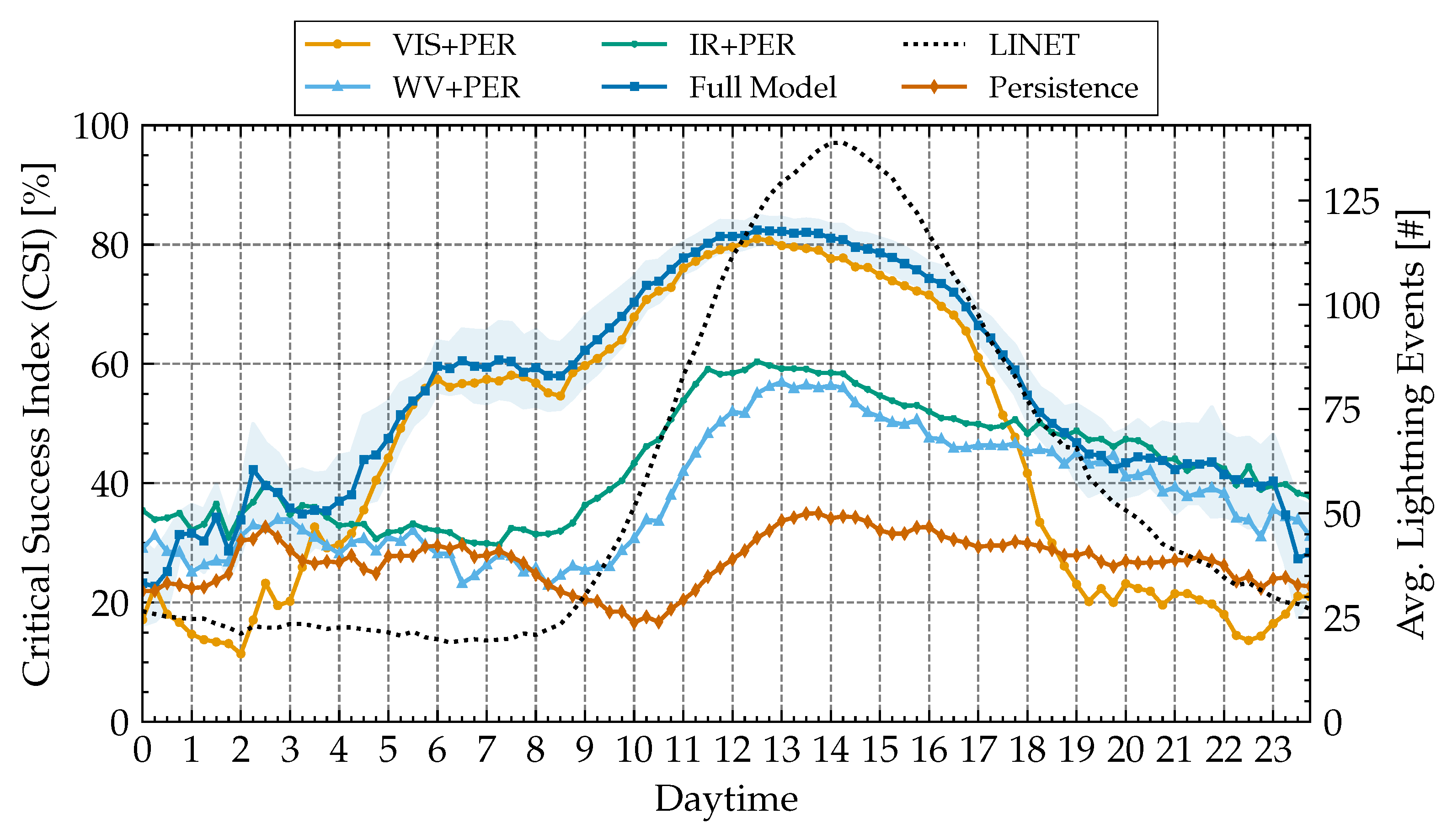
Figure 6 shows the result of training the classifier again, but with some inputs omitted. The graph shows the CSI over the course of the day, with an overlay of the number of lightning events recorded by LINET (dotted black curve) at these times of day on average (clearly peaking in the afternoon UTC time, which is late afternoon local time in the observed region). The time on the x-axis denotes to the prediction time and corresponds to the number of lightning events shown (the actual data used for the prediction are taken 2 h prior).
The full classifier model (dark blue curve) shows a significantly lower CSI at night-time than during the day: With the sunrise starting, performance improves, and drops again later in the evening; the increase in performance during 4–6 am UTC coincides with the beginning of dawn in Central Europe (local daylight-saving time being offset by +2 h) in the relevant time frame of May to August. As more daylight becomes available closer to the start of summer, more visible information becomes available earlier in the day, which could explain the transition in accuracy. Similarly, accuracy declines towards the end of the day.
A second phenomenon, apparently overlayed with the hypothesized daylight effect, is a further increase in CSI between 9 and 16 h UTC, peaking around noon (notably, at about 80% CSI). This corresponds to the time where most LINET events have been recorded. Apparently, prediction becomes easier if events are more common (which is a statistically plausible finding and would be expected).
The hypothesis that the network bases its decision mostly on information in the visible spectrum of light is solidified by looking at the CSI-curves when using only images from the visible spectrum (VIS/light orange) versus various infrared channels only (light blue/green): During daylight, the model using only visible features drops only slightly in performance compared to the full model (often within the 1 σ -margin of error of the full model), while the infrared models perform significantly worse. Only at night, the prediction benefits from IR-information (with visible-only falling behind), although at an overall poorer level of performance. Surprisingly, the water-vapor bands alone yield an even slightly worse performance than the other IR-channels.
The comparison against base-line persistence shows an occasional drop below base-line for the restricted models, which might be explained by training noise (with variance increasing during low-event-count night times); this also suggests to not over-interpret smaller differences (WV vs. IR), but the gap to visible light appears very large and correspondingly very unlikely coincidental.
In summary, we observe that visible light has by far the largest contribution to classification performance, indicating the image recognition in the visible spectrum plays a major role. When visible light is available, the model performs very well at levels of CSI of 60–80%, which might have some operational relevance for applications to daytime activities. Infrared imagery appears to be much less informative to our classifier, which can only sustain a generally lower prediction performance consistently at day and night times. The water vapor channels alone, which are a target for physically motivated, “hand-crafted” models [12], lead to overall worse prediction results than visible or other infrared bands.

4. Conclusions

Our paper provides an end-to-end training technique for Cb nowcasting. As it works directly on unbalanced data, it can easily be used for predictions, as no pre-filtering of data is required. The experimental results provide clear indications that deep learning can be used to improve the Cb nowcasting even in this general scenario of naturally unbalanced classes. It should be noted, however, that the data used are not maximally unbalanced: All training and testing has so far been taken from the “warm” months of May to September, where lightning is much more prevalent in the observed region of Central Europe; including winter data and/or a more global excerpt of the planet might likely lead to a decrease in performance.
Comparison to operational nowcasting approaches: Most physical models are based on the extrapolation of the detected Cbs with atmospheric motion vectors (AMV; see [14] and the references therein). This approach works well as long as the cells do not decay during the prediction period. Unfortunately, cells usually do decay after a certain lifetime, such that this effect occurs regularly. Further, newly developed cells cannot be captured by extrapolation of detected cells. These are serious drawbacks of the AMV approach. The quite good results achieved with deep learning indicate that the training process might enable the network to gain information on the life cycles of cells (decay, newly developed cells). The network seems to be able to learn to a certain extent whether Cbs decay or newly develop within the prediction period or not, and we believe this is crucial for lead times around or larger than 180 min, as the lifetime of regular Cbs is usually shorter than this; see, e.g., [50].
Importance of the visible-light spectrum: The results diagrammed in Figure 6 clearly show that the learning process benefits tremendously from the visible channels. In the IR, only the cloud top contributes to the emission and hence to the signal measured at the satellite, with exception of semi-transparent clouds. However, in the VIS, the complete cloud contributes to the signal, and the reflections hold the information of the cloud optical thickness and effective cloud droplet radii [51]. Thus, the VIS provide much more information about the cloud textures, shapes and micro physics. It is likely that this information is used to learn information about the life cycle of Cbs. Otherwise, better results compared to physical methods are hard to explain. Although the prediction of Cbs with NWP has been significantly improved, nowcasting is still assumed to outperform NWP in the first 0–3 h. Thus, a lot of scientists aim to develop a seamless transition between nowcasting and NWP. Currently, mainly physical methods are used to achieve this goal, but deep learning might be a powerful alternative.

Author Contributions

Conceptualization, S.B. and M.W.; Data Curation, S.B. and R.M.; Formal Analysis, S.B.; Funding Acquisition, P.S.; Investigation, S.B.; Methodology, S.B.; Project Administration, E.S., P.S. and M.W.; Resources, E.S., P.S. and M.W.; Software, S.B.; Supervision, E.S. and M.W.; Validation, S.B. and R.M.; Visualization, S.B.; Writing—Original Draft, S.B., R.M. and M.W.; Writing—Review and Editing, S.B., R.M., E.S., P.S. and M.W. All authors have read and agreed to the published version of the manuscript.

Funding

This research has been partially funded by the Carl-Zeiss-Stiftung (grant no. P2018-02-003, “Big Data in Atmospheric Physics (BINARY)”).

Data Availability Statement

Restrictions apply to the availability of the used data. Meteosat SEVIRI image data were obtained from EUMETSAT and are available at https://navigator.eumetsat.int/product/EO:EUM:DAT:MSG:HRSEVIRI (accessed on 14 June 2022). LINET lightning data were obtained from DWD.

Acknowledgments

The study is supported by the project “Big Data in Atmospheric Physics (BINARY)”, funded by the Carl-Zeiss-Stiftung (grant P2018-02-003). We acknowledge the DWD for providing access to the LINET data. We acknowledge EUMETSAT for providing access to the Meteosat SEVIRI image data. We acknowledge the ZDV of the Johannes Gutenberg University and the Mogon II Super Cluster for providing the necessary hardware, computing time, and storage to prepare our experiments. We thank David Hartmann for fruitful discussions.

Conflicts of Interest

The authors declare no conflict of interest.

Abbreviations

The following abbreviations are used in this manuscript:
ABIAdvanced baseline imager
AIArtificial intelligence
ANNArtificial neural network
BTBrightness temperature
CbCumulonimbus cloud (incl. thunderstorms and lightning)
CECross entropy (loss function)
CIConvective initiation
CRSCoordinate reference system
CSICritical success index
DWDDeutscher Wetterdienst (German Weather Service)
FARFalse alarm ratio
FEDFlash-extent density
FNFalse negative
FPFalse positive
GLD360Vaisala global lightning detection network
GLMGeostationary lightning mapper
HRITHigh rate image transmission
IFImprovement factor
IRInfrared
LRLearning rate
LRRTLearning rate range test
MRMSMulti-radar multi-sensor
MSGMeteosat second generation
NWPNumerical weather prediction
PODProbability of detection
ROIRegion of interest
SEVIRISpinning enhanced visible and infrared imager
SGDWStochastic gradient descent with momentum using decoupled weight decay
SSPSub-satellite point
TNTrue negative
TOATime-of-arrival
TPTrue positive
WDWeight decay
WVWater vapor

Appendix A

Appendix A.1. Data Set Splits

Detailed information about the data and their use can be seen in Table A1 and Table A2 for 2016/2017 and 2021, respectively. We focus our work on the summer months May to August in the years of 2016 and 2017. As additional test data set, we use data from August and September of 2021. We split the data based on weeks, and assign each to a different data set (shown in column “Data Set”). To uniformly cover the complete time span of the 2016/17 data with every data set, we assign successive weeks to alternating, repetitive sets of “train”, “test”, “train”, “validation”, and so on. This culminates in 19 train, 10 test, and 9 validation “weeks” for the 2016/17 period, and 10 weeks of testing data for the 2021 period (which is solely used for testing purposes). A 12 h window between weeks is discarded to prevent temporal “data leakage” between sets.
Table A1. Train, test, and validation splits for 2016/2017 data set. Events are shown in millions ( × 10 6 ) in the area ( 2 . 0 W– 21 . 5 E, 44 . 5 N– 57 . 5 N).
YearMonthWeekEventsData Set
2016May17 0.03 Train
2016May18 0.10 Test
2016May19 0.24 Train
2016May20 0.13 Validation
2016May21 0.70 Train
2016May/June22 0.94 Test
2016June23 0.80 Train
2016June24 0.56 Validation
2016June25 1.81 Train
2016June/July26 0.58 Test
2016July27 0.36 Train
2016July28 1.08 Validation
2016July29 0.70 Train
2016July30 1.18 Test
2016August31 0.95 Train
2016August32 0.28 Validation
2016August33 0.67 Train
2016August34 0.50 Test
2016August35 0.56 Train
2017May17 0.01 Validation
2017May18 0.15 Train
2017May19 0.26 Test
2017May20 0.28 Train
2017May21 0.33 Validation
2017May/June22 1.10 Train
2017June23 0.37 Test
2017June24 0.61 Train
2017June25 1.88 Validation
2017June/July26 1.05 Train
2017July27 0.81 Test
2017July28 0.77 Train
2017July29 1.29 Validation
2017July30 1.13 Train
2017July/August31 0.89 Test
2017August32 1.25 Train
2017August33 0.45 Validation
2017August34 0.43 Train
2017August/September35 0.95 Test
Table A2. Additional test split for 2021 data set. Events are shown in millions ( × 10 6 ) in the area ( 2 . 0 W– 21 . 5 E, 44 . 5 N– 57 . 5 N).
YearMonthWeekEventsData Set
2021July30 0.23 Test
2021August31 1.09 Test
2021August32 1.06 Test
2021August33 0.89 Test
2021August34 1.33 Test
2021August/September35 0.82 Test
2021September36 0.97 Test
2021September37 0.56 Test
2021September38 0.88 Test
2021September/October39 0.29 Test

Appendix A.2. Critical Success Index Calculation

We evaluate the performance of our method and the baseline method by calculating the critical success index (CSI) [52,53], similar to previous works, e.g., [12,54]. The CSI is the amount of correct classified events out of all events classified and undetected events. A natural question that arises is how to combine multiple CSI values of different samples to form a single performance measure.
We define the (combined) Critical Success Index (CSI) of all samples in a data set Ω as
CSI Ω = s Ω TP ( s ) s Ω TP ( s ) + s Ω FN ( s ) + s Ω FP ( s ) ,
where TP, FN, and FP are the true positives, false negatives, and false positive of a sample, respectively. This way, we always measure the performance for an entire data set by combining all events from all samples. This differs from classical machine-learning tasks, e.g., image classification, where a more fine-grained performance measure that combines each individual measure of each sample is used.

Appendix A.3. Domain-Decomposition

Domain decomposition has become an essential tool in large-scale computation over the past decades because of its use to solve problems on parallel machines in the context of physical simulations [55]. In our case, a trade-off arises between the precision of the representation (or the level of detail) of the phenomenon and the memory and computer performance required to compute the model. We aim to fully capture the spatial context in the input patch, using the highest level of detail. To maintain viable memory and compute requirements, we apply a domain decomposition scheme to split the input in smaller subdomains. This allows us to split the computational workload and process the smaller subdomains, without excluding regions.
Figure A1 shows an example of the used domain decomposition. Here, the original domain (347 px × 654 px; 17.35° × 32.7°; ca. 1929 km × 3636 km) (grayscale image) is split into six subdomains (256 px × 256 px; 12.8° × 12.8°; ca. 1423 km × 1423 km). The boundary (overlapping) region is marked in blue, consisting of a padding of 16 px ( 0.8 ° ; ca. 88 km) around the non-overlapping subdomain, which is shown in orange. The boundary region allows a more precise prediction at regions at the edge of the orange subdomain, because the cause of occurring lightning might lie outside of it. With a boundary width of roughly 88 km and a time discretization of 15 min of the satellite imagery, clouds with a horizontal speed of up to 100 m   s 1 are visible during their transition through the boundary region.
Figure A1. Example of the applied domain decomposition scheme into six slightly overlapping subdomains, shown for VIS006 (grayscale), 20160604 12:00 UTC. The non-overlapping regions are shown in orange, and their boundary (overlapping) regions are shown in blue.
Remotesensing 14 03760 g0a1
To ensure all subdomains have the same size, the original domain is padded with zeros to the needed size, which is shown as white ”background“ in Figure A1. Pixels in these padded regions are excluded from the optimization process and evaluation of our method.

Appendix A.4. Improvement Factor

During our research, we found it very difficult to (directly) compare our work with similar methods. The reasons for this were the under-specification of the metrics used to report the results, the lack of access to the used data, and the lack of availability of the code necessary for evaluation. Thus, we were unable to reproduce the reported results and evaluate our method in the same way, which seems to be a general problem in machine-learning research [56,57].
Therefore, we compare our method against a baseline method using a naive forecast with the “persistence” algorithm and compute the improvement factor (IF) of our method over the given baseline. The persistence algorithm is a model in which each lightning is assumed to be lighting in the same location and the same intensity as it was at the last known time step. Thus, the Cbs remain at their original position throughout the prediction time; hence, no forecast is applied and the Cbs are assumed to be static, which can be seen in Figure 5c. This deterministic method requires no training, is fast to implement with no significant additional compute, and is often already available in the literature.
The improvement factor (IF) of a method α over method β is defined as
IF ( α , β ) = CSI α CSI β ,
in particular, the IF over the persistence model is given as IF ( α , PERSISTENCE ) .
By computing the IF over the persistence model, we are able to compare our work with others, where otherwise no direct comparison would be possible, e.g., due to a different implementation of the CSI, or a deviation in ROI. In this way, we can improve the comparison between studies.
Table A3 shows the CSI of the persistence model used for the calculation of the improvement factor. Figure 5d shows the skill for a severe weather event (4 June 2016 [49]).
Table A3. CSI of the persistence model for various data sets, SR 30.61 k m , and varying lead time (LT).
Data Split\LT0 min30 min60 min90 min120 min180 min
Validation 16/17 100.00 81.38 56.11 38.08 27.73 17.10
Testing 16/17 100.00 80.89 58.42 40.37 28.64 16.11
Testing 21 August 100.00 78.66 48.79 31.01 21.36 12.25
Testing 21 September 100.00 80.08 57.03 39.50 28.42 16.79

Appendix A.5. Learning Rate Schedule

Figure A2 shows the learning rate (LR) schedule throughout the training process. The schedule is set using a 1-cycle LR scheduler [47] with two phases using cosine decay. The training starts with an LR of 0.05 ( 1 10 of the base LR), which then increases to the maximum LR of 0.5 (base LR) at a training progress of about 20 % (beginning of epoch 3). Over the course of the remaining 80 % of the training progress, the LR is decayed to the minimum LR of 0.0005 ( 1 1000 of the base LR). This schedule is calculated at the start of the training process and is not altered during training. The maximum LR was experimentally chosen by running the learning rate range test (LRRT) [58], which is a method for discovering the largest possible learning rates one can use to train a model “successfully”. While linearly increasing the learning rate, we examined the divergence of the loss, and additionally, the changes in the mean activation pattern temperature of the network [59].
Figure A2. Detailed learning rate schedule throughout the training process.
Remotesensing 14 03760 g0a2

References

  1. Saunders, C. Charge separation mechanisms in clouds. In Planetary Atmospheric Electricity; Springer: Berlin, Germnay, 2008; pp. 335–353. [Google Scholar]
  2. Pruppacher, H.R.; Klett, J.D. Microphysics of Clouds and Precipitation. In Atmospheric and Oceanographic Sciences Library; Kluwer Academic Publishers: Dordrecht, The Netherlands, 2010; Volume 18. [Google Scholar]
  3. Zängl, G.; Reinert, D.; Rípodas, P.; Baldauf, M. The ICON (ICOsahedral Non-hydrostatic) modelling framework of DWD and MPI-M: Description of the non-hydrostatic dynamical core. Q. J. R. Meteorol. Soc. 2015, 141, 563–579. [Google Scholar] [CrossRef]
  4. Reinert, D.; Prill, F.; Frank, H.; Denhard, M.; Baldauf, M.; Schraff, C.; Gebhardt, C.; Marsigli, C.; Zängl, G. DWD Database Reference for the Global and Regional ICON and ICON-EPS Forecasting System; Technical Report Version 2.1.7; DWD: Frankfurt, Germany, 2021. [Google Scholar]
  5. Schmid, F.; Wang, Y.; Harou, A. Nowcasting Guidelines–A Summary. Bull. N° 2019, 68, 2. [Google Scholar]
  6. Mass, C. Nowcasting: The Promise of New Technologies of Communication, Modeling, and Observation. Bull. Am. Meteorol. Soc. 2012, 93, 797–809. [Google Scholar] [CrossRef] [Green Version]
  7. Oprea, S.; Martinez-Gonzalez, P.; Garcia-Garcia, A.; Castro-Vargas, J.A.; Orts-Escolano, S.; Rodríguez, J.G.; Argyros, A.A. A Review on Deep Learning Techniques for Video Prediction. arXiv 2020, arXiv:2004.05214. [Google Scholar] [CrossRef] [PubMed]
  8. Betz, H.; Schmidt, K.; Oettinger, W.; Montag, B. Cell-tracking with lightning data from LINET. Adv. Geosci. 2008, 17, 55–61. [Google Scholar] [CrossRef] [Green Version]
  9. Fortun, D.; Bouthemy, P.; Kervrann, C. Optical flow modeling and computation: A survey. Comput. Vis. Image Underst. 2015, 134, 1–21. [Google Scholar] [CrossRef] [Green Version]
  10. James, P.; Reichert, B.; Heizenreder, D. NowCastMIX: Automatic Integrated Warnings for Severe Convection on Nowcasting Time Scales at the German Weather Service, Weather and Forecasting. Weather Forecast. 2018, 33, 1413–1433. [Google Scholar] [CrossRef]
  11. Schmetz, J.; Tjemkes, A.; Gube, M.; van der Berg, L. Monitoring deep convection and convective overshooting with Meteosat. Adv. Space Res. 1997, 19, 433–441. [Google Scholar] [CrossRef]
  12. Müller, R.; Haussler, S.; Jerg, M.; Heizenreder, D. A Novel Approach for the Detection of Developing Thunderstorm Cells. Remote Sens. 2019, 11, 443. [Google Scholar] [CrossRef] [Green Version]
  13. Cintineo, J.L.; Pavolonis, M.J.; Sieglaff, J.M.; Wimmers, A.; Brunner, J.; Bellon, W. A Deep-Learning Model for Automated Detection of Intense Midlatitude Convection Using Geostationary Satellite Images. Weather Forecast. 2020, 35, 2567–2588. [Google Scholar] [CrossRef]
  14. Müller, R.; Barleben, A.; Haussler, S.; Jerg, M. A Novel Approach for the Global Detection and Nowcasting of Deep Convection and Thunderstorms. Remote Sens. 2022, 14, 3372. [Google Scholar] [CrossRef]
  15. Lee, Y.; Kummerow, C.D.; Ebert-Uphoff, I. Applying machine learning methods to detect convection using Geostationary Operational Environmental Satellite-16 (GOES-16) advanced baseline imager (ABI) data. Atmos. Meas. Tech. 2021, 14, 2699–2716. [Google Scholar] [CrossRef]
  16. Autones, F. Algorithm Theoretical Basis Document for Convection Products; Technical report; NWC-SAF (METEO-FRANCE): Toulouse, France, 2016. [Google Scholar]
  17. Gijben, M.; Coning, C. Using Satellite and Lightning Data to Track Rapidly Developing Thunderstorms in Data Sparse Regions. Atmosphere 2017, 8, 67. [Google Scholar] [CrossRef] [Green Version]
  18. Schön, C.; Dittrich, J.; Müller, R. The Error is the Feature: How to Forecast Lightning using a Model Prediction Error. In Proceedings of the 25th ACM SIGKDD International Conference on Knowledge Discovery & Data Mining, KDD 2019, Anchorage, AK, USA, 4–8 August 2019; Teredesai, A., Kumar, V., Li, Y., Rosales, R., Terzi, E., Karypis, G., Eds.; ACM: New York, NY, USA, 2019; pp. 2979–2988. [Google Scholar] [CrossRef] [Green Version]
  19. Mecikalski, J.R.; Williams, J.K.; Jewett, C.P.; Ahijevych, D.; LeRoy, A.; Walker, J.R. Probabilistic 0–1-h convective initiation nowcasts that combine geostationary satellite observations and numerical weather prediction model data. J. Appl. Meteorol. Climatol. 2015, 54, 1039–1059. [Google Scholar] [CrossRef] [Green Version]
  20. Zhou, K.; Zheng, Y.; Dong, W.; Wang, T. A Deep Learning Network for Cloud-to-Ground Lightning Nowcasting with Multisource Data. J. Atmos. Ocean. Technol. 2020, 37, 927–942. [Google Scholar] [CrossRef]
  21. Deng, J.; Dong, W.; Socher, R.; Li, L.J.; Li, K.; Fei-Fei, L. Imagenet: A large-scale hierarchical image database. In Proceedings of the 2009 IEEE Conference on Computer Vision and Pattern Recognition, Miami Beach, FL, USA, 20–25 June 2009; IEEE: Piscataway, NJ, USA, 2009; pp. 248–255. [Google Scholar]
  22. Krizhevsky, A.; Sutskever, I.; Hinton, G.E. ImageNet Classification with Deep Convolutional Neural Networks. In Advances in Neural Information Processing Systems; Pereira, F., Burges, C.J.C., Bottou, L., Weinberger, K.Q., Eds.; Curran Associates, Inc.: Red Hook, NY, USA, 2012; Volume 25. [Google Scholar]
  23. He, K.; Zhang, X.; Ren, S.; Sun, J. Deep Residual Learning for Image Recognition. In Proceedings of the 2016 IEEE Conference on Computer Vision and Pattern Recognition (CVPR), Las Vegas, NV, USA, 27–30 June 2016; pp. 770–778. [Google Scholar] [CrossRef] [Green Version]
  24. Ronneberger, O.; Fischer, P.; Brox, T. U-Net: Convolutional Networks for Biomedical Image Segmentation. In Lecture Notes in Computer Science, Proceedings of the Medical Image Computing and Computer-Assisted Intervention—MICCAI 2015—18th International Conference, Munich, Germany, 5–9 October 2015; Part III; Navab, N., Hornegger, J., Wells, M.W., Frangi, A.F., Eds.; Springer: Berlin/Heidelberg, Germany, 2015; Volume 9351, pp. 234–241. [Google Scholar] [CrossRef] [Green Version]
  25. Dewitte, S.; Cornelis, J.; Müller, R.; Munteanu, A. Artificial Intelligence Revolutionises Weather Forecast, Climate Monitoring and Decadal Prediction. Remote Sens. 2021, 13, 3209. [Google Scholar] [CrossRef]
  26. Hoeser, T.; Künzer, C. Object Detection and Image Segmentation with Deep Learning on Earth Observation Data: A Review-Part I: Evolution and Recent Trends. Remote Sens. 2020, 12, 1667. [Google Scholar] [CrossRef]
  27. Hoeser, T.; Bachofer, F.; Kuenzer, C. Object Detection and Image Segmentation with Deep Learning on Earth Observation Data: A Review - Part II: Applications. Remote Sens. 2020, 12, 3053. [Google Scholar] [CrossRef]
  28. Ma, L.; Liu, Y.; Zhang, X.; Ye, Y.; Yin, G.; Johnson, B.A. Deep learning in remote sensing applications: A meta-analysis and review. ISPRS J. Photogramm. Remote Sens. 2019, 152, 166–177. [Google Scholar] [CrossRef]
  29. Boukabara, S.A.; Krasnopolsky, V.; Stewart, J.Q.; Maddy, E.S.; Shahroudi, N.; Hoffman, R.N. Leveraging Modern Artificial Intelligence for Remote Sensing and NWP: Benefits and Challenges. Bull. Am. Meteorol. Soc. 2019, 100, ES473–ES491. [Google Scholar] [CrossRef]
  30. Ayzel, G.; Scheffer, T.; Heistermann, M. RainNet v1.0: A convolutional neural network for radar-based precipitation nowcasting. Geosci. Model Dev. 2020, 13, 2631–2644. [Google Scholar] [CrossRef]
  31. Lebedev, V.; Ivashkin, V.; Rudenko, I.; Ganshin, A.; Molchanov, A.; Ovcharenko, S.; Grokhovetskiy, R.; Bushmarinov, I.; Solomentsev, D. Precipitation Nowcasting with Satellite Imagery. In Proceedings of the 25th ACM SIGKDD International Conference on Knowledge Discovery & Data Mining, KDD 2019, Anchorage, AK, USA, 4–8 August 2019; Teredesai, A., Kumar, V., Li, Y., Rosales, R., Terzi, E., Karypis, G., Eds.; ACM: New York, NY, USA, 2019; pp. 2680–2688. [Google Scholar] [CrossRef] [Green Version]
  32. Agrawal, S.; Barrington, L.; Bromberg, C.; Burge, J.; Gazen, C.; Hickey, J. Machine Learning for Precipitation Nowcasting from Radar Images. arXiv 2019, arXiv:1912.12132. [Google Scholar]
  33. Shi, X.; Gao, Z.; Lausen, L.; Wang, H.; Yeung, D.; Wong, W.; Woo, W. Deep Learning for Precipitation Nowcasting: A Benchmark and A New Model. In Proceedings of the Advances in Neural Information Processing Systems 30: Annual Conference on Neural Information Processing Systems 2017, Long Beach, CA, USA, 4–9 December 2017; Guyon, I., von Luxburg, U., Bengio, S., Wallach, H.M., Fergus, R., Vishwanathan, S.V.N., Garnett, R., Eds.; Curran Associates, Inc.: Red Hook, NY, USA, 2018; pp. 5617–5627. [Google Scholar]
  34. Han, D.; Lee, J.; Im, J.; Sim, S.; Lee, S.; Han, H. A Novel Framework of Detecting Convective Initiation Combining Automated Sampling, Machine Learning, and Repeated Model Tuning from Geostationary Satellite Data. Remote Sens. 2019, 11, 1454. [Google Scholar] [CrossRef] [Green Version]
  35. Mostajabi, A.; Finney, D.L.; Rubinstein, M.; Rachidi, F. Nowcasting lightning occurrence from commonly available meteorological parameters using machine learning techniques. Npj Clim. Atmos. Sci. 2019, 2, 1–15. [Google Scholar] [CrossRef]
  36. EUMETSAT. High Rate SEVIRI Level 1.5 Image Data—MSG—0 Degree. Available online: https://navigator.eumetsat.int/product/EO:EUM:DAT:MSG:HRSEVIRI (accessed on 14 June 2022).
  37. Brodehl, S. pyPublicDecompWT: Python Bindings for EUMETSAT’s PublicDecompWT (v2.8.1.3). Available online: https://pypi.org/project/pyPublicDecompWT (accessed on 14 June 2022).
  38. Raspaud, M.; Hoese, D.; Lahtinen, P.; Finkensieper, S.; Holl, G.; Proud, S.; Dybbroe, A.; Meraner, A.; Feltz, J.; Zhang, X.; et al. Pytroll/Satpy, Version 0.36.0 (2022/04/14). Available online: https://iopscience.iop.org/article/10.1088/1755-1315/750/1/012011/meta (accessed on 14 June 2022).
  39. Hoese, D.; Lahtinen, P.; Raspaud, M.; Roberts, W.; Lavergne; Bot, S.; Finkensieper, S.; Dybbroe, A.; Holl, G.; Itkin, M.; et al. Pytroll/Pyresample, Version 1.23.0. Available online: https://www.preprints.org/manuscript/202206.0238/v1 (accessed on 14 June 2022).
  40. Met Office. Cartopy: A Cartographic Python Library with a Matplotlib Interface. 2010–2015. Available online: https://scitools.org.uk/cartopy (accessed on 14 June 2022).
  41. Cui, Y.; Jia, M.; Lin, T.; Song, Y.; Belongie, S.J. Class-Balanced Loss Based on Effective Number of Samples. In Computer Vision Foundation, Proceedings of the IEEE Conference on Computer Vision and Pattern Recognition, CVPR 2019, Long Beach, CA, USA, 16–20 June 2019; IEEE: Piscataway, NJ, USA, 2019; pp. 9268–9277. [Google Scholar] [CrossRef] [Green Version]
  42. He, K.; Zhang, X.; Ren, S.; Sun, J. Identity Mappings in Deep Residual Networks. In Lecture Notes in Computer Science, Proceedings of the Computer Vision - ECCV 2016—14th European Conference, Amsterdam, The Netherlands, 11–14 October 2016; Part IV; Leibe, B., Matas, J., Sebe, N., Welling, M., Eds.; Springer: Berlin, Germany, 2016; Volume 9908, pp. 630–645. [Google Scholar] [CrossRef] [Green Version]
  43. Ulyanov, D.; Vedaldi, A.; Lempitsky, V.S. Instance Normalization: The Missing Ingredient for Fast Stylization. arXiv 2016, arXiv:1607.08022. [Google Scholar] [CrossRef]
  44. Nair, V.; Hinton, G.E. Rectified Linear Units Improve Restricted Boltzmann Machines. In Proceedings of the 27th International Conference on Machine Learning (ICML-10), Haifa, Israel, 21–24 June 2010; Fürnkranz, J., Joachims, T., Eds.; Omnipress: Madison, WI, USA, 2010; pp. 807–814. [Google Scholar]
  45. Rumelhart, D.E.; Hinton, G.E.; Williams, R.J. Learning representations by back-propagating errors. Nature 1986, 323, 533–536. [Google Scholar] [CrossRef]
  46. Loshchilov, I.; Hutter, F. Decoupled Weight Decay Regularization. In Proceedings of the 7th International Conference on Learning Representations, ICLR 2019, New Orleans, LA, USA, 6–9 May 2019. [Google Scholar]
  47. Smith, L.N.; Topin, N. Super-Convergence: Very Fast Training of Residual Networks Using Large Learning Rates. arXiv 2017, arXiv:1708.07120. [Google Scholar] [CrossRef]
  48. Paszke, A.; Gross, S.; Massa, F.; Lerer, A.; Bradbury, J.; Chanan, G.; Killeen, T.; Lin, Z.; Gimelshein, N.; Antiga, L.; et al. PyTorch: An Imperative Style, High-Performance Deep Learning Library. arXiv 2019, arXiv:1912.01703. [Google Scholar] [CrossRef]
  49. Klimaveränderung und Wasserwirtschaft (KLIWA). Klimawandel in Süddeutschland—Veränderung von Meteorologischen und Hydrologischen Kenngrößen; Monitoringbericht 2016. Available online: https://www.kliwa.de/_download/KLIWA_Monitoringbericht_2016.pdf (accessed on 14 June 2022).
  50. Lang, T.J.; Miller, L.J.; Weisman, M.; Rutledge, S.A.; Barker, L.J., III; Bringi, V.; Chandrasekar, V.; Detwiler, A.; Doesken, N.; Helsdon, J.; et al. The severe thunderstorm electrification and precipitation study. Bull. Am. Meteorol. Soc. 2004, 85, 1107–1126. [Google Scholar] [CrossRef] [Green Version]
  51. Nakajima, T.; King, M.D. Determination of the Optical Thickness and Effective Particle Radius of Clouds from Reflected Solar Radiation Measurements. Part I: Theory. J. Atmos. Sci. 1990, 47, 1878–1893. [Google Scholar] [CrossRef] [Green Version]
  52. Schaefer, J.T. The Critical Success Index as an Indicator of Warning Skill. Weather Forecast. 1990, 5, 570–575. [Google Scholar] [CrossRef] [Green Version]
  53. Gerapetritis, H.; Pelissier, J.M. On the Behavior of the Critical Success Index, Eastern Region Technical Attachment (National Weather Service (U.S.)); No. 2004-03; NOAA/National Weather Service: Greer, South Carolina, 2004. [Google Scholar]
  54. Ravuri, S.; Lenc, K.; Willson, M.; Kangin, D.; Lam, R.; Mirowski, P.; Fitzsimons, M.; Athanassiadou, M.; Kashem, S.; Madge, S.; et al. Skilful precipitation nowcasting using deep generative models of radar. Nature 2021, 597, 672–677. [Google Scholar] [CrossRef] [PubMed]
  55. Dolean, V.; Jolivet, P.; Nataf, F. An Introduction to Domain Decomposition Methods—Algorithms, Theory, and Parallel Implementation; SIAM: Philadelphia, PA, USA, 2015. [Google Scholar]
  56. Pineau, J.; Vincent-Lamarre, P.; Sinha, K.; Larivière, V.; Beygelzimer, A.; d’Alché-Buc, F.; Fox, E.B.; Larochelle, H. Improving Reproducibility in Machine Learning Research (A Report from the NeurIPS 2019 Reproducibility Program). J. Mach. Learn. Res. 2021, 22, 1–20. [Google Scholar]
  57. Garg, S.; Rasp, S.; Thuerey, N. WeatherBench Probability: A benchmark dataset for probabilistic medium-range weather forecasting along with deep learning baseline models. arXiv 2022, arXiv:2205.00865. [Google Scholar] [CrossRef]
  58. Smith, L.N. Cyclical Learning Rates for Training Neural Networks. In IEEE Computer Society, Proceedings of the 2017 IEEE Winter Conference on Applications of Computer Vision, WACV 2017, Santa Rosa, CA, USA, 24–31 March 2017; IEEE: Piscataway, NJ, USA, 2017; pp. 464–472. [Google Scholar] [CrossRef] [Green Version]
  59. Hartmann, D.; Brodehl, S.; Wand, M. ActCooLR—High-Level Learning Rate Schedules Using Activation Pattern Temperature. 2021. Available online: https://openreview.net/forum?id=yqj6q_eNTJd (accessed on 14 June 2022).
Figure 1. SEVIRI satellite images (in radiances) (bd) and (aggregated and binarized) LINET events (a) for Central Europe on 4 June 2016 at 12:00 UTC. In the IR120 (d) (WV062, (c)) only the cloud top contributes to the emission and hence to the signal measured at the satellite, with exception of semi-transparent clouds. However, in the VIS (b) the complete cloud contributes to the signal. The texture, thickness and shape of clouds are therefore much more pronounced in the VIS.
Remotesensing 14 03760 g001
Figure 2. Illustration of the used network architecture, based on a U-Net with residual blocks. Depicted in light gray is the tensor size ( H , W , T ) between each block; the batch size and the number of channels have been omitted. Blue boxes correspond to down-sampling residual blocks, green boxes correspond to up-sampling residual blocks, and dark gray boxes correspond to residual blocks. Dashed lines indicate skip connections between the encoding and decoding phases of the U-Net. Solid lines indicate connections between layers.
Remotesensing 14 03760 g002
Figure 3. Detailed illustration of the used architecture blocks of our network, used for down- (a) and up-sampling (b), as well as a residual block (c). Down-sampling is realised with strided convolutions, whereas deterministic up-sampling is used. Concatenation of tensors in the channel dimension is denoted as ∘. Addition of tensors of the same size is denoted as +.
Remotesensing 14 03760 g003
Figure 4. Improvement factor (right y-axis) and CSI (left y-axis) over lead time: Performance measures using CSI for a search radius of 30.61 km of our method for various data sets. All lines showing the improvement factor start at the bottom-left, and all lines showing the CSI start at the top-left.
Remotesensing 14 03760 g004
Figure 5. Predictions and skill of the compared methods for a 120 min forecast during a severe weather event, 4. June 2016 12:00 UTC. (a): Unscaled model logits. Sharp lines at around 11°E, 26°E and 43°N are artifacts from the domain decomposition scheme, detailed in Appendix A.3. (b): Model skill: CSI 77.82 %, POD 78.25 %, FAR 21.74 %. (c): Persistence predictions. Cbs remain static, no forecast is applied. (d): Persistence skill: CSI 43.46 %, POD 60.86 %, FAR 39.13 %. True positives are marked green, false positives orange, and false negatives purple.
Remotesensing 14 03760 g005
Figure 6. CSI over daytime (left y-axis): Performance measures for 120 min forecasts using CSI for search radius 30.61 k m of our method for the 2016/2017 test data sets, using only VIS+PER ( VIS 0.6 , VIS 0.8 , nIR 1.6 , Persistence ), WV+PER ( WV 6.2 , WV 7.3 , Persistence ) and IR+PER ( IR 3.9 , IR 8.7 , IR 9.7 , IR 10.8 , IR 12.0 , IR 13.4 , Persistence ) channels. Average lightning events over daytime (right y-axis).
Remotesensing 14 03760 g006
Table 2. Measured class-weight of the training split for the 2016/2017 data set.
ClassClass-Weight
lightning 0.15
no-lightning 99.85
Table 3. Detailed number of channels in the network, depending on the lead time.
Lead TimeBlock 1Block 2Block 3Block 4Block 5Block 6Bottleneck
0 min 13131414151616
30 min 14162028468181
60 min 14162131529797
90 min 1416213256106106
120 min 1416223359114114
180 min 1416223563124124
Table 4. Detailed training settings, depending on lead time and network size.
Lead TimeBottleneck ChannelsBase LRWDRegularization FactorEpochs
0 min 160.55.0 × 10−60.114
30 min 810.57.0 × 10−60.1514
60 min 970.57.0 × 10−60.214
90 min 1060.57.0 × 10−60.214
120 min 1140.51.0 × 10−50.314
180 min 1240.51.0 × 10−50.314
Table 5. CSI of our method for various data sets, SR 30.61 k m and varying lead time (LT).
Data Split\LT0 min30 min60 min90 min120 min180 min
Validation 16/17 99.9 ± 0.0 89.2 ± 0.8 78.5 ± 1.6 74.4 ± 1.6 66.8 ± 2.9 38.2 ± 2.3
Testing 16/17 99.7 ± 0.0 88.6 ± 1.4 77.8 ± 1.9 76.2 ± 1.6 70.0 ± 2.7 41.8 ± 3.1
Testing August 21 99.9 ± 0.0 87.9 ± 1.1 75.4 ± 2.0 69.7 ± 2.7 61.3 ± 3.7 31.9 ± 3.0
Testing September 21 99.1 ± 0.0 87.2 ± 1.3 72.9 ± 2.7 66.9 ± 3.5 56.9 ± 5.2 24.7 ± 4.2
Publisher’s Note: MDPI stays neutral with regard to jurisdictional claims in published maps and institutional affiliations.

