Smart Count System Based on Object Detection Using Deep Learning

Abstract

Object counting is an indispensable task in manufacturing and management. Recently, the development of image-processing techniques and deep learning object detection has achieved excellent performance in object-counting tasks. Accordingly, we propose a novel small-size smart counting system composed of a low-cost hardware device and a cloud-based object-counting software server to implement an accurate counting function and overcome the trade-off presented by the computing power of local hardware. The cloud-based object-counting software consists of a model adapted to the object-counting task through a novel DBC-NMS (our own technique) and hyperparameter tuning of deep-learning-based object-detection methods. With the power of DBC-NMS and hyperparameter tuning, the performance of the cloud-based object-counting software is competitive over commonly used public datasets (CARPK and SKU110K) and our custom dataset of small pills. Our cloud-based object-counting software achieves an mean absolute error (MAE) of 1.03 and a root mean squared error (RMSE) of 1.20 on the Pill dataset. These results demonstrate that the proposed smart counting system accurately detects and counts densely distributed object scenes. In addition, the proposed system shows a reasonable and efficient cost–performance ratio by converging low-cost hardware and cloud-based software.

1. Introduction

The necessity of counters in various manufacturing industries has been highlighted by mass production [1,2,3]. Owing to the fact that most of the preceding counters used for manufacturing usually count only a single type of product, it was necessary to develop a different counter for each product when dealing with various types of merchandise. Hence, various studies on general-purpose counters have been conducted over the years. Sensor-based counters [4] are popular. Sensors are sensitive to external conditions; thus, most sensor-based counters are designed for a specifically structured environment to achieve high accuracy. Therefore, these methods are not universal and are not comparable to other methods.

In recent years, owing to the advancements in image-processing techniques, counters using image sensors have been developed [5,6,7,8,9,10,11,12,13,14,15,16,17,18]. In the early stages, the objects were counted by extracting their edges. In this case, the condition that the objects should be clearly distinguished from the background was essential. In contrast, recent deep-learning-based counters have the advantage of being able to detect objects robustly in any environment, provided they have been trained by a sufficient amount of data. However, these object-detection models still have limitations in that they do not perform sufficiently when the density of objects in the image is high. To overcome this limitation, we propose a novel counting system by combining the existing object-detection model and our distance between circles nonmaximum suppression (DBC-NMS) technique.

In addition to software, the corresponding hardware device is just as important to enable the whole process of counting objects. Mazzia et al. [19] proposed a real-time apple-detection system. This system utilized YOLO v3-tiny [20], which is a relatively small device, to run a deep-learning-based detector on a low-cost embedded platform. Horng et al. [21] proposed a harvesting system that detected and classified crop ripeness. This system includes an external server for the object detectors MobileNet2 [22] and SSD [23]. However, the approach proposed in [19] has the limitation of being hardware-dependent, and that proposed in [21] is limited by the fact that it detects objects well but is not optimized for counting. In summary, a counter that is optimized for object counting and implemented not only in software but also in hardware has never been proposed.

The main contributions of this paper are summarized as follows:

1.

We propose a novel object-counting method by applying our new object-counting technique (DBC-NMS) to an existing state-of-the-art deep learning object-detection model (CenterNet2) and hyper-parameter tuning.

2.

Our cloud-based deep learning software server showcases consistent performance regardless of hardware device specifications. This means that many clients can handle our server at a low cost, and the more that clients use our server, the more our server becomes specialized for a specific domain through staged fine-tuning processes.

3.

We demonstrate the potential of our smart counting system as a general-purpose counting device by realizing a pipeline of all the processes to the hardware system that can operate in conjunction with the cloud-based deep learning software server. Additionally, we propose a semi-automated object-collecting process to assist in the rapid removal of excessive objects.

The remainder of this paper is organized as follows. Section 2 reviews related works related to counters as well as deep-learning-based object detection. Section 3 discusses the details of the object-detection server and local hardware device. In Section 4, the object-detection models used for the object-detection server are evaluated and the overall performance of the proposed smart counting system is verified. Finally, Section 5 concludes the paper.

2. Related Works

2.1. Deep-Learning-Based Counting

Deep-learning-based object-counting methods can be roughly classified into four categories: regression-based, density-map-estimation-based, heatmap-estimation-based, and object-detection-based methods.

Regression-based methods (Wang et al. [8] and Xue et al. [9].) count objects by mapping high-dimensional images into a real number space through regression models. Wang et al. proposed an end-to-end deep convolutional neural network regression model for counting people in images. Xue et al. proposed a regression model that counted the number of cells by cropping the image into patches. These methods have difficulties with objects of varying scales and cluster distributions. This regression-based approach predicts a scalar count for an input image without explicit object localization information.

Density-map-estimation-based method (Lempitsky et al. [10]) set a milestone for density-map-estimation-based counting studies by casting the object-counting problem in an image as a density map estimation, in which the integral of the density map provided the count of objects within it. Zhang et al. [11] proposed a multi-column neural network (MCNN) with three columns, each column consisting of CNNs of different kernel sizes, to estimate density maps for objects of different sizes. Sindagi et al. [12] improved the MCNN by learning it as a classification problem with density map estimation for the crowd-counting task, and integrated it into an end-to-end cascading network. Gao et al. [13] proposed ASPDNet, which introduced a feature pyramid network and deformable convolution network, and integrated the attention mechanism.

Heatmap-estimation-based method (Kilic et al. [14]) is a new CNN model called the heatmap learner convolutional neural network (HLCNN), which generated heatmaps for car locations. HLCNN casts the object-counting problem in an image as a heatmap estimation, which provides the count of objects within the heatmap.

Object-detection-based method employing object-detection networks, such as Faster-RCNN [24], YOLO [25,26,27,28], SSD [23], RetinaNet [29], and CenterNet [30], have shown state-of-the-art performance in many object-detection tasks. Counting is completed spontaneously after detection by summarizing the number of detection instances. These methods and variants have shown promising results, such as those reported by Hsieh et al. [15], Goldman et al. [16], Li et al. [31], and Cai et al. [17], for car counting in aerial images. Wang et al. [18] proposed a new self-learning approach called crowd-SDNet to estimate both the centroid and size of a crowded object.

2.2. Object Detectors

A recent deep-learning-based object detector is typically composed of two parts: a backbone and a head. The backbone of the detector is generally pretrained on ImageNet [32]. VGG [33], ResNet [34], DenseNet [35], ResNeXt [36], and EfficientNet [37] are used as the backbone. In addition, for detectors running on low-cost hardware, MobileNet [38] or SqueezeNet [39] can be used as the backbone. The head of the detector is used to predict the bounding boxes and classes of objects. Depending on the head, the detectors can be classified into two types: one-stage and two-stage detectors.

In two-stage detectors, the first stage detects potential objects and their locations, and the second stage classifies these potential objects. During training, the first stage is designed to maximize the recall, and the second stage is designed to maximize the classification objective. The regions with convolutional neuron networks features (R-CNN) series—which includes R-CNN [40], fast R-CNN [41], faster R-CNN [24], and mask R-CNN [42]—are representative two-stage detectors.

One-stage detectors mainly predict object location and class likelihood and learn by maximizing the local likelihood of annotated ground truth objects during training. Well-known one-stage detectors include SSD [23], YOLO [25,26,27,28], and RetinaNet [29]. CornerNet [43] and CenterNet [30] are one-stage detectors that use keypoint estimation for object detection. In YOLOR [44], Wang et al. proposed a unified network for encoding implicit and explicit knowledge together.

CenterNet2 [45], which a is state-of-the-art, probabilistic, two-stage detector that complements the limitations of the two-stage detector, mapping the class probability of the basic one-stage detector and the k bounding boxes taken from the shared head of the model, such as two-stage detectors. In Section 3.1.1, we analyze each object detector in more detail to select a model suitable for our system in tackling the object-counting task.

3. The Proposed Smart Counting System

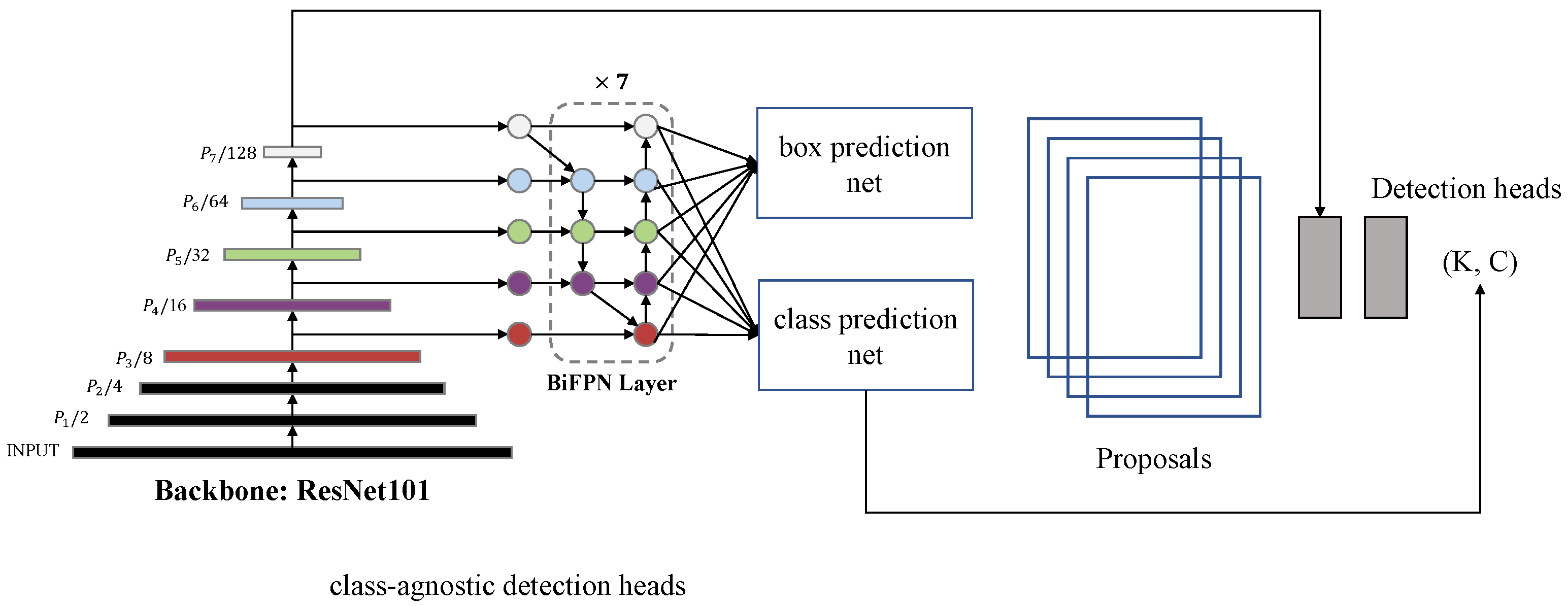
3.1. Object-Detection Configurations for the Object-Counting Task

3.1.1. Analysis of the Object Detectors

Object-detection methods encounter difficulties in detecting heavily compacted scenes. Therefore, their performance on the COCO test set [46], an object-detection benchmark, was used to adopt an object-detection model that was suitable for count tasks.

A representative model of a one-stage detector, YOLO [25,26,27,28], divides an image into cell units. This limits its performance when objects are concentrated within the size of a cell unit. Furthermore, models using many types of anchor boxes [25,26,27,28] have a limitation in that an imbalance occurs between positive and negative anchor boxes. To solve this problem, focal loss has been added [29], but it requires the optimization of hyper-parameters, such as the intersection over union (IoU) threshold suitable for dataset tasks, anchor box size, and ratio.

However, CornerNet [43] and CenterNet [30] use key point estimation, which makes grouping and postprocessing unnecessary. CornerNet predicts a bounding box by detecting two corners (upper left and lower right) as key points, and CenterNet predicts each object as a single point by using the center point as a key point. CenterNet2 [45], a probabilistic two-stage detector, adds a cascade RoI head [47] on top of the first-stage proposal network, as shown in Figure 1, and is both faster and more accurate than its one- or two-stage counterparts, that is, CenterNet. Methods using keypoint estimation [30,43,45] show no degradation in their performance, even in situations where objects are dense (small objects heavily packed in compact scenes).

Cloud-based software supplements computing power beyond the hardware potential of the system. Therefore, we employ CenterNet2 as the object-detection model of the proposed system, which shows the best mAP and adequate FPS in the COCO benchmark, as shown in

Table 1. Performance of object detectors on COCO test-dev. ( ) means the backbone of the model. Frames per second (FPS) of every detector were measured on a machine with NVIDIA RTX 2080 TI.

Object Detector	mAP	FPS
	(Mean Average Precision)	(Frames per Second)
Faster RCNN [24]	39.8	9.4
Tiny YOLO [25]	23.7	33.6
YOLO9000 [26]	21.9	9.5
RetinaNet (ResNet101-FPN) [29]	40.8	5.4
YOLOv3 (Darknet-53) [27]	33.0	20
CornerNet (Hourglass-104) [43]	42.1	4.1
CenterNet (Hourglass-104) [30]	45.1	7.8
YOLOv4 (CSPDarknet-53) [28]	43.5	33
CenterNet2 (ResNet101-BiFPN) [45]	56.4	33
Swin-T (cascade mask RCNN) [48]	50.5	5.3
YOLOR [44]	52.6	47.5

, among the competitive object detectors.

3.1.2. DBC-NMS (Distance between Circles—NMS)

Nonmaximum suppression (NMS) is an essential part of an object-detection pipeline. It helps match a bounding box of each object from the predicted result of an image. The traditional NMS algorithm calculates the ratio between the intersection and union areas (i.e., the IoU) of two bounding boxes and compares it with the previously defined IoU threshold to determine the degree of overlap between the two boxes. However, in this case, depending on the orientation of the object, the area occupied by the actual object may be significantly smaller than that of the bounding box. In other words, a large error occurs in the bounding box. Because of the error, area-based postprocessing causes erroneous results, as shown in Figure 2. For example, if the threshold of NMS is strictly set as shown in Figure 2a, then even the correctly predicted box is removed. On the other hand, if the threshold of NMS is set loosely, as shown in Figure 2b, then it is impossible to remove the wrongly predicted box. This means that, even if the IoU threshold value is adjusted, accurate prediction is difficult because of the error introduced by the bounding box.

To address this problem, we propose DBC-NMS, a distance-based postprocessing method. As shown in Figure 2c, DBC-NMS redefines a circle from the bounding box so that the degree of overlap can be determined regardless of the orientation of the object. The circle is defined to have a radius, $r_i$, which is the distance from the center points of the bounding box. $r_i$ is computed based on the width and height values of the bounding box and $\epsilon$, as follows:

$$r_i=\frac{min(b_{i,width},b_{i,height})}{2}\epsilon .$$

(1)

where $\epsilon$ is a value that adjusts the size of the circle (the effect of $\epsilon$ is examined in Section 4.6). Using the circles, the degree of overlap between objects is determined as follows:

$$s_i=\left\{\begin{array}{c}{s}_i,\hspace{1em}Euclidean\_Distance(c_m,c_i)>r_m+r_i\\ 0,\hspace{1em}Euclidean\_Distance(c_m,c_i)\le r_m+r_i\end{array}\right..$$

(2)

Circles in which the Euclidean distance between the center points is less than the sum of the radii are removed and considered as the same object. Therefore, only the maximum score between the overlapped circles remains, and the rest are removed. In the converse case, each circle is considered as an independent object. Figure 3a shows a situation in which both bounding boxes are maintained as they indicate two different objects, and Figure 3b shows a situation in which one bounding box with a low score is removed as it is considered to indicate the same object. The overall DBC-NMS process is shown in Algorithm 1.

Algorithm 1 Pseudo code of DBC-NMS
Input:
$\mathbf{B}=\left[b_1,\cdots b_n\right]$	▹$\mathbf{B}$ is the list of initial detection boxes
$\mathbf{S}=\left[s_1,\cdots s_n\right]$	▹$\mathbf{S}$ contains corresponding detection scores
$\epsilon$	▹$\epsilon$ is the DBC-NMS threshold
1: procedureDBC-NMS($\mathbf{B},\mathbf{S},\epsilon$) 2:     $\mathit{Pick}\leftarrow \left\{\right\}$ 3:     $\mathbf{C}=\left[c_1,\cdots c_n\right]={\mathbf{B}}_{center\_point}$ 4:     $\mathbf{R}=\left[r_1,\cdots r_n\right]=\frac{min({\mathbf{B}}_{width},{\mathbf{B}}_{height})}{2}\epsilon$ 5:     $\mathbf{I}=\mathit{argsort}\mathbf{S}$ 6:      while len($\mathbf{I})>0$  do 7:         $m\leftarrow \mathbf{I}.pop\left(\right)$ 8:         $\mathit{Pick}\leftarrow \mathit{Pick}\cup \left\{m\right\}$ 9:         $\mathit{Keep}\leftarrow \left[\right]$ 10:          for i in $\mathbf{I}$  do 11:             if $Euclidean\_Distance(c_m,c_i)>r_m+r_i$  then 12:                $\mathit{Keep}$.append(i) 13:         $\mathbf{I}\leftarrow \mathit{Keep}$ 14:      return $\mathbf{B}\left[\mathit{Pick}\right]$, $\mathbf{S}\left[\mathit{Pick}\right]$

3.2. Cloud-Based Software Server

3.2.1. Architecture

The server for object detection uses AWS cloud resources, as shown in Figure 4. The object-detection model is configured with Docker so that it can be simply deployed on top of the default AWS Deep Learning AMI environment at an AWS EC2 GPU instance. In addition, the EC2 instance is created as an auto-scaling group to facilitate expansion according to the number of users.

The cloud-based object-detection server communicates with Raspberry Pi through a socket connection for fast data transmission and reception. The EC2 instance of the server receives an image from Raspberry Pi and returns the center coordinates of the items, according to the request of the user. The returned value is displayed to the client using a web-based UI. In addition, as the user collects the counted items, the image and prediction results are stored as pairs in AWS S3. With the selected model, CenterNet2, the FPS of the entire pipeline, including all low-cost hardware and cloud-based software, has been measured as 3.47.

3.2.2. Staged Fine-Tuning

We adopt a stagewise training method to effectively optimize the model to the task with minimal data annotation. First, a neural network pretrained with the COCO dataset is fine-tuned on a handful of data, which is manually composed. Subsequently, the fine-tuned model is served temporarily through the cloud server to obtain more data for further fine-tuning stages. Then, from AWS S3 storage, the input images and the corresponding model predictions are obtained and postprocessed for use as the dataset of the next fine-tuning stage. After a few repetitions of fine-tuning, a task-optimized model is obtained. The stem and second stage of the backbone model are frozen to prevent overfitting. The experiments of our stagewise training method are described in Section 4.7.

3.3. Local Hardware Device

The local hardware device is designed using AutoCAD, as described in Figure 5a, and the entire structure is assembled from aluminum profiles, as shown in Figure 5b. The tray used for collecting the objects is fabricated using a 3D printer. A low-cost embedded board, Raspberry Pi 4 model B with 8gb memory, is employed as the main computer of this device. It receives images from the camera, exchanges data with the cloud-based object detection server, deploys a web application, highlights the items to be removed by controlling the beam projector, and collects items by actuating a motor. A mini DLP beam projector SC497 is used as the beam projector, and a Logitech Pro Stream webcam C922 is employed as the camera. To align the beam projector and the camera angle, the camera is set vertically to view the tray, as shown in Figure 5c. In addition, the beam projector is adjusted to an angle of view, which prevents interference with the camera. To collect items, a basic Raspberry Pi servo motor is used. The rotational motion generated by the motor is converted to linear motion through a crank, shaft, and connecting rod, as shown in Figure 6. Owing to the circular bar inserted in the middle of the tray, the converted linear motion is once again converted into rotational motion, which allows the objects to fall.

3.4. Web-Based UI

We configured a web-based user interface (UI) such that users can easily check the counted results in the smart counting system. The UI, implemented as a web application, can be connected through various devices, such as PCs, smartphones, and tablet PCs. The UI flow is described by Algorithm 2. First, after setting $target\_qty$, the web-based UI notifies the user whether the quantity is insufficient or excessive by comparing it with the predicted results of the object-detection server. If $target\_qty<current\_qty$, then the  beam projector highlights the items to be removed, and users can easily remove them. Otherwise, if $target\_qty>current\_qty$, then the UI notifies the user that there should be more items.

Algorithm 2 Smart count system-UI algorithm

1: procedure 2:     $target\_qty\leftarrow$ desired object quantity 3:     $current\_qty\leftarrow$ predicted object quantity from detection server 4:      if $target\_qty>0$  then 5:          while $target\_qty!=current\_qty$  do 6:             if $target\_qty<current\_qty$  then 7:                Remove recommended items 8:             else if $target\_qty>current\_qty$  then 9:                Add items to tray 10:             if The button ’collect anyway’ is pushed then 11:                 break 12:          if The button ’collect’ is pushed then 13:            Collect items

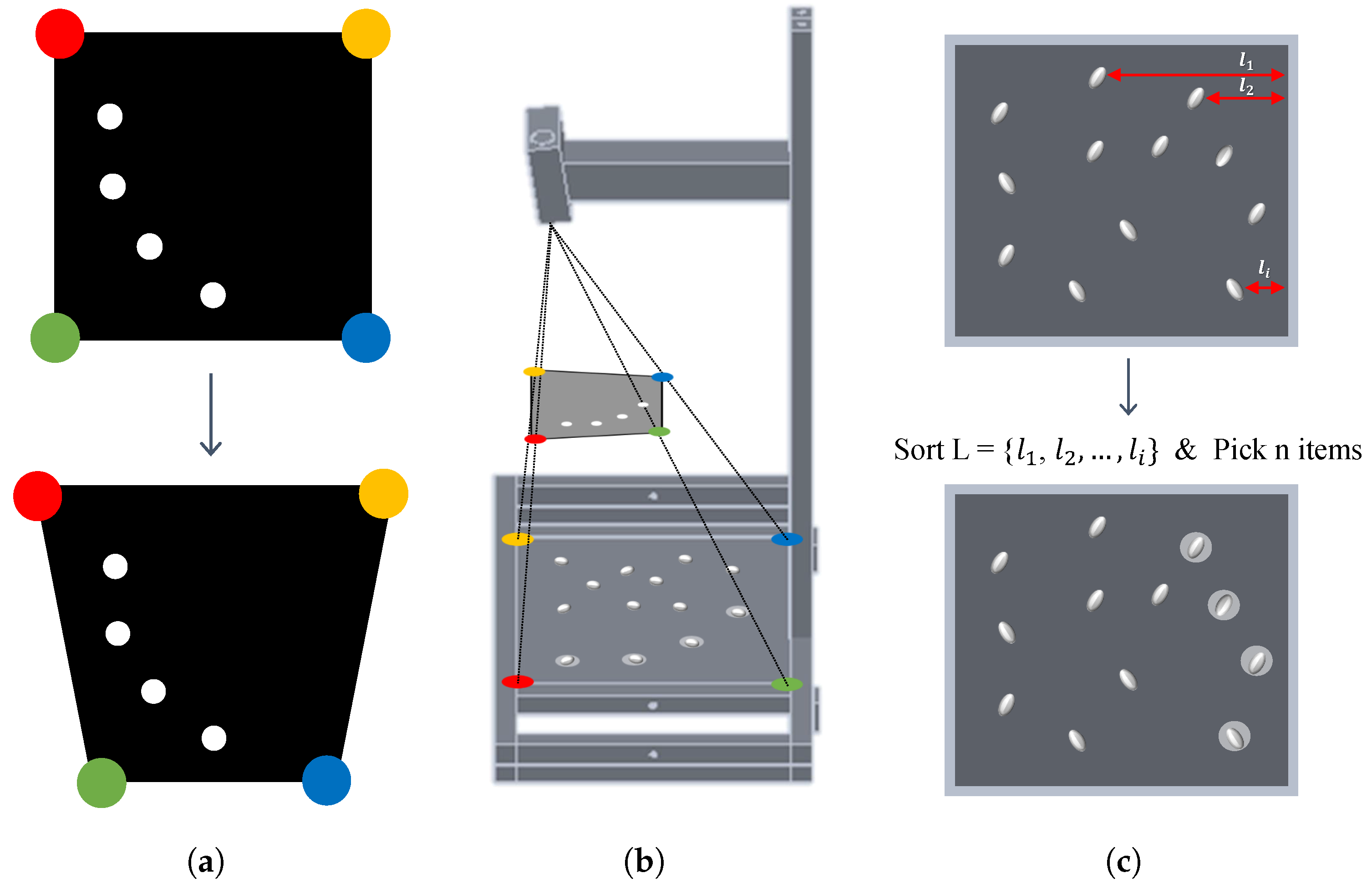
3.5. Beam Projector Transformation

Owing to the installed angle of the beam projector, the projected image is distorted. A perspective transform [49] is used to match the exact location of the excessive objects, as shown in Figure 7. The perspective transformation linearly transforms the distorted image to match the position of each corner of the tray.

3.6. Semi-Automated Counting and Collecting Process

For a faster removal of excessive items, our semi-automated counting process recommends items to be removed. The recommended items are selected from the right side of the tray, and their positions are calibrated to project a bright circle for each item with the beam projector, as shown in Figure 7b. In addition, if the user pushes the “collect” button on the UI, the motor is actuated through PWM control of the Raspberry Pi. The motor adjusts the angle of the tray to drop items simultaneously. The overall process of the smart counting system is illustrated in Figure 8. The first step is to place the items on the tray and input the desired quantity in the UI of the system. The UI is implemented as a web application, and users can access it using any device, including mobile devices. Then, when the image taken from the top of the tray is sent to the server, the server-side object-detection software counts the number of items on the image and notifies the user as to whether the quantity is insufficient or excessive. If the quantity of items is excessive, then the system recommends the items to be removed and displays them on the UI screen, simultaneously highlighting them on the tray using the mounted beam projector, as shown in Figure 7c. Finally, if the number of items matches the input, then the items are collected using the system actuator.

4. Experimental Results and Analysis

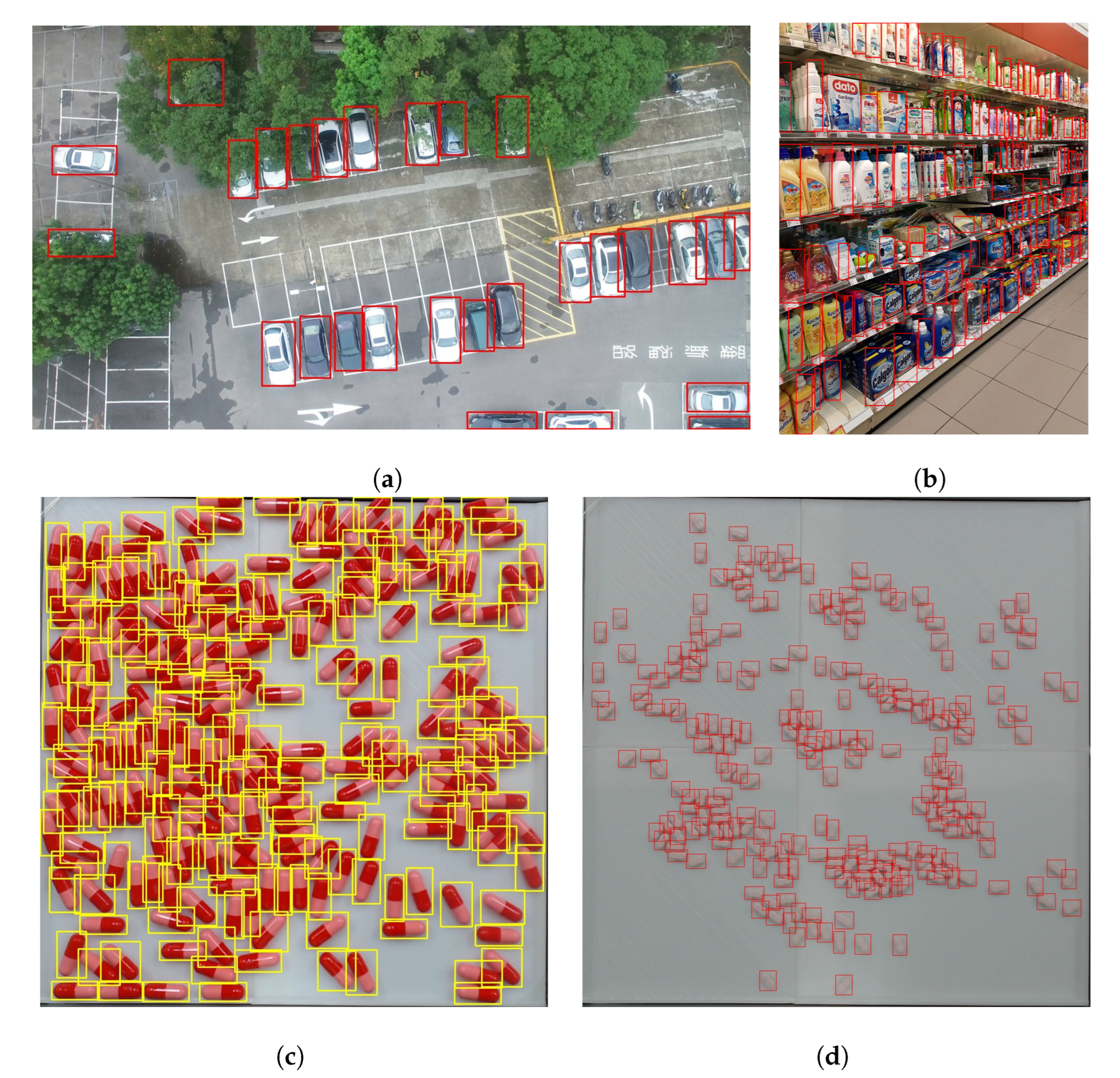
In this section, we first elaborate on the experimental settings, including the datasets, evaluation metrics, and implementation details. We also compare our smart counting system with previous works [14,16,18] on three datasets. Quantitative experiments were conducted to validate the proposed system.

4.1. Datasets

We evaluated our proposed method using three counting datasets: CARPK [15], SKU-110K [16], and Pill (our custom dataset). The details of each dataset are as follows.

CARPK [15] is a well-known public benchmark for object counting that is composed of drone-viewed images of vehicles parked in parking lots. It contains nearly 90,000 cars in four different parking lots and is split into 989 training and 459 testing datasets. A sample image of the CARPK dataset is shown in Figure 9a.

SKU-110K [16] is a public counting benchmark that contains images of supermarket shelves. Each image contains various densely packed products, as shown in Figure 9b. It consists of 11,762 images, which are split into 8233 images for training, 588 images for validation, and 2941 images for testing.

The Pill dataset is a custom dataset for counting pills, as shown in Figure 9c,d. We assembled this new labeled dataset to evaluate the counting performance for small and densely packed objects. It consists of 14,000 images, 12,000 for training and 2000 for testing, and each image is packed with 1–937 pills. We constructed a dataset containing various shapes and colors of pills to consider the diversity of pills. All images were captured at a distance of 2–40 cm from the tray and collected using the hardware device of our system described in Section 3.3.

4.2. Evaluation Metrics

We adopted commonly used metrics in object-counting tasks: mean absolute error (MAE) and root mean squared error (RMSE) [12,13,14,15,16,18,50]. The metrics are expressed as numerical values, and are used to quantify the difference between the ground truths and predicted results. The value approaches zero as it matches the ground truth. The MAE indicates the accuracy of the models and is defined as follows:

$$\mathrm{MAE}=\frac{1}{n}\sum _{i=1}^n\left|N_G-N_P\right|,$$

(3)

where n is the number of images, $N_G$ is the number of ground-truth objects, and $N_P$ is the predicted number of objects. The RMSE indicates the robustness of the models and is formulated as follows:

$$\mathrm{RMSE}=\sqrt{\frac{1}{n}\sum _{i=1}^n{\left(N_G-N_P\right)}^2}.$$

(4)

4.3. Implementation Details

The basic code for CenterNet2 was based on the official paper code. The CenterNet2 backbone, Res2Net-101-DCN-BiFPN, was initialized with pretrained weights of CenterNet2_R2-101-DCN-BiFPN_4x+4_1560_ST from the official code. For the DBC-NMS parameter, $\epsilon$ is set to 0.2 in all experiments. The detector was trained on two GPUs with a batch size of eight. An SGD optimizer was used with a base learning rate of 0.01. All fine-tuning was trained for 30 epochs, and flip augmentation was used with an image size of 640 × 640. All counting methods were implemented based on the official code of the paper.

4.4. Comparison with Existing Works

Our method was compared with three existing methods [14,16,18] on the CARPK, SKU-110K, and Pill datasets. These methods have shown the best performance on CARPK and SKU110k in the previous studies. The experimental results are listed in

Table 2. Count task comparisons with existing works.

Method	CARPK		SKU110k		Pill
	MAE	RMSE	MAE	RMSE	MAE	RMSE
Goldman et al. [16]	6.77	8.52	14.52	24.00	11.01	19.29
Wang et al. [18]	4.95	7.09	26.78	40.66	1.32	2.09
Kilic et al. [14]	2.12	3.02	14.74	27.54	6.70	13.37
CenterNet2 [45] + DBC-NMS (ours)	3.53	4.77	12.72	21.59	1.03	1.20

. CARPK consists of frames extracted from videos captured by drones, as shown in Figure 9a. As data are captured from continuous frames, objects at the edges of the images are partially visible, and objects under the trees are heavily obscured. Therefore, the heatmap approach achieves lower MAE and RMSE compared with the object-detection approaches. Kilicm et al., whose paper proposed an HLCNN that generated heatmaps for car locations, achieved 2.12 MAE and 3.02 RMSE, which are 1.41 and 1.75 lower than those of our method. SKU-110K consists of images that contain heavily packed items, and only the items in the front line among the displayed items are considered objects. In this case, as shown in Figure 9b, counting objects is a very challenging task. Accordingly, the MAE and RMSE results of all the methods tend to have high values. Of all the methods, our method performed best, with an MAE of 12.72 and an RMSE of 21.59. On the Pill dataset, our method also shows the lowest MAE and RMSE, which is 0.29 and 0.89 lower than the second lowest one obtained by Wang et al. [18]. Therefore, it is verified that the proposed method effectively counts objects, even in densely packed tasks with complex backgrounds.

4.5. The Effectiveness of the DBC-NMS

In this section, to prove the effectiveness of DBC-NMS, we compared it with traditional NMS and Soft-NMS, which have been widely used, for three methods [16,18,45]. NMS is a postprocessing process for object-detection results; therefore, only approaches using object-detection methods were compared. The first block in

Table 3. Performance of DBC-NMS.

Method	CARPK		SKU110k		Pill
	MAE	RMSE	MAE	RMSE	MAE	RMSE
Goldman et al. [16] + NMS	6.77	12.00	14.52	24.00	11.01	19.29
Wang et al. [18] + NMS	7.28	9.30	27.85	49.96	1.32	2.09
CenterNet2 [45] + NMS	3.72	4.81	13.27	21.99	1.08	1.25
Goldman et al. + Soft-NMS	6.52	10.93	14.28	24.02	6.81	12.10
Wang et al. + Soft-NMS	4.95	7.09	26.78	40.66	1.32	2.09
CenterNet2 + Soft-NMS	3.60	4.78	13.05	21.83	1.04	1.23
Goldman et al. + DBC-NMS	6.22	10.93	14.24	24.00	6.79	12.07
Wang et al. + DBC-NMS	5.64	7.14	22.97	34.19	1.24	1.98
CenterNet2 + DBC-NMS (ours)	3.53	4.77	12.72	21.59	1.03	1.20

shows the performance of the reference methods with traditional NMS. The second block shows the performance of the methods with Soft-NMS [51], and the last block shows the performance of the methods using the DBC-NMS. DBC-NMS showed better performance than NMS and Soft-NMS in most experiments. Validated by the results, our DBC-NMS algorithm can filter overlapped objects and shows potential as a postprocessing method for count tasks.

4.6. Sensitivity Analysis of Parameter $\epsilon$ for DBC-NMS

To evaluate the performance of DBC-NMS according to epsilon, we conducted experiments with $\epsilon$ values ranging from 0.15 to 0.45 on the Pill dataset. Figure 10 shows the performance change according to epsilon for the three models compared in Section 4.5. Goldman et al. showed better performance of 7.024 MAE and 12.307 RMSE for $\epsilon$ = 0.2 compared with other $\epsilon$ values. In the cases of Wang et al. and CenterNet2, $\epsilon$ = 0.35 produced better results with 1.245 MAE and 1.982 RMSE and 1.05 MAE and 1.202 RMSE, respectively.

Examining the performance change according to the epsilon of the three models, it is verified that, in general, the results with $\epsilon$ from 0.2 to 0.4 are similar. In other words, the proposed DBC-NMS requires less effort for parameter tuning than the conventional NMS.

4.7. Staged Fine-Tuning

Figure 11 shows the performance of the staged fine-tuning, as mentioned in Section 3.2.2. The first stage was fine-tuned with a no-base, manually processed dataset, and the remaining stages were fine-tuned with a preprocessed dataset, which was reworked from the prediction of the previous stage’s fine-tuned model. The first stage achieved 100.508 for the MAE and 128.856 for the RMSE with 100 datasets; therefore, reworking the predictions of the model requires significant manual effort. The second stage, fine-tuned with 500 datasets, was 98.829 and 125.632 lower for the MAE and RMSE than the first stage, respectively. With a considerably low error from the second stage, the reworking dataset requires significantly less manual effort, and repeated fine-tuning from the preprocessed dataset, at the fifth stage yields an MAE of 1.05 and an RMSE of 1.202. Therefore, 500 datasets were considered as the minimum for a task-optimized model. As the number of datasets increases, the range of model improvement decreases, but with our cloud-based deep learning software server and staged fine-tuning, datasets can be easily gathered, and less manual effort is required to process the data.

4.8. Scenario

Figure 12 shows snapshots of the scenarios shown in

Table 4. Our scenario.

Scenario
1. Place object on tray.	(a)
2. Write your target quantity and press “Count!” button.
3. Check the current quantity and remove excess items.
(Excess objects are marked with white circles.)	(b)
4. Although 11 objects need to be removed, we removed 13 for example.
5. Press “Collect” button.
6. User Warning for target quantity mismatch.
7. Check the current quantity and add insufficient items.	(c)
8. Press “Collect” button and collect items through motor control.	(d)

. To demonstrate the capabilities of the web-based UI and smart counting system, a scenario was carried out assuming that the object was removed excessively. The full video can be viewed through the following link, https://youtu.be/Ox2XAM5OaR0 (accessed on 1 August 2022). The video as well as snapshots showed that the proposed smart system successfully counted the objects not only accurately but also robustly.

5. Conclusions

We proposed a novel, small-sized smart counting system with a cloud-based object-counting software server, consisting of an object-detection model and DBC-NMS. The proposed system overcomes the trade-off of computing power of local hardware and can count various object types by stagewise fine-tuning the cloud-based object-counting server with a specific task dataset. Through a web-based UI, the results can be easily verified using mobile devices. Finally, a semi-automated counting process that matches a desired quantity faster and more accurately than counting by hand is realized. As a result, our counter showed competitive performance as a device specializing in counting and collecting small-sized objects.

References

1. Phromlikhit, C.; Cheevasuvit, F.; Yimman, S. Tablet counting machine base on image processing. In Proceedings of the 5th 2012 Biomedical Engineering International Conference, Muang, Thailand, 5–7 December 2012; pp. 1–5. [Google Scholar]
2. Furferi, R.; Governi, L.; Puggelli, L.; Servi, M.; Volpe, Y. Machine vision system for counting small metal parts in electro-deposition industry. Appl. Sci. 2019, 9, 2418. [Google Scholar] [CrossRef] [Green Version]
3. Nudol, C. Automatic jewel counting using template matching. In Proceedings of the IEEE International Symposium on Communications and Information Technology, 2004, ISCIT 2004, Sapporo, Japan, 26–29 October 2004; Volume 2, pp. 654–658. [Google Scholar]
4. Sun, F.J.; Li, S.; Xu, H.H.; Cai, J.D. Design of counting-machine based on CCD sensor and DSP. Transducer Microsyst. Technol. 2008, 4, 103–104. [Google Scholar]
5. Venkatalakshmi, B.; Thilagavathi, K. Automatic red blood cell counting using hough transform. In Proceedings of the 2013 IEEE Conference on Information & Communication Technologies, Thuckalay, India, 11–12 April 2013; pp. 267–271. [Google Scholar]
6. Gu, Y.; Li, L.; Fang, F.; Rice, M.; Ng, J.; Xiong, W.; Lim, J.H. An Adaptive Fitting Approach for the Visual Detection and Counting of Small Circular Objects in Manufacturing Applications. In Proceedings of the 2019 IEEE International Conference on Image Processing (ICIP), Taipei, Taiwan, 22–25 September 2019; pp. 2946–2950. [Google Scholar]
7. Baygin, M.; Karakose, M.; Sarimaden, A.; Akin, E. An image processing based object counting approach for machine vision application. arXiv 2018, arXiv:1802.05911. [Google Scholar]
8. Wang, C.; Zhang, H.; Yang, L.; Liu, S.; Cao, X. Deep people counting in extremely dense crowds. In Proceedings of the 23rd ACM international conference on Multimedia, Brisbane, Australia, 26–30 October 2015; pp. 1299–1302. [Google Scholar]
9. Xue, Y.; Ray, N.; Hugh, J.; Bigras, G. Cell counting by regression using convolutional neural network. In Proceedings of the European Conference on Computer Vision; Springer: Berlin/Heidelberg, Germany, 2016; pp. 274–290. [Google Scholar]
10. Lempitsky, V.; Zisserman, A. Learning to count objects in images. Adv. Neural Inf. Process. Syst. 2010, 23, 1324–1332. [Google Scholar]
11. Zhang, Y.; Zhou, D.; Chen, S.; Gao, S.; Ma, Y. Single-image crowd counting via multi-column convolutional neural network. In Proceedings of the IEEE Conference on Computer Vision and Pattern Recognition, Las Vegas, NV, USA, 27–30 June 2016; pp. 589–597. [Google Scholar]
12. Sindagi, V.A.; Patel, V.M. Cnn-based cascaded multi-task learning of high-level prior and density estimation for crowd counting. In Proceedings of the 2017 14th IEEE International Conference on Advanced Video and Signal Based Surveillance (AVSS), Lecce, Italy, 29 August–1 September 2017; pp. 1–6. [Google Scholar]
13. Gao, G.; Liu, Q.; Wang, Y. Counting From Sky: A Large-Scale Data Set for Remote Sensing Object Counting and a Benchmark Method. IEEE Trans. Geosci. Remote Sens. 2020, 59, 3642–3655. [Google Scholar] [CrossRef]
14. Kilic, E.; Ozturk, S. An accurate car counting in aerial images based on convolutional neural networks. J. Ambient. Intell. Humaniz. Comput. 2021, 1–10. [Google Scholar] [CrossRef]
15. Hsieh, M.R.; Lin, Y.L.; Hsu, W.H. Drone-based object counting by spatially regularized regional proposal network. In Proceedings of the IEEE International Conference on Computer Vision, Venice, Italy, 22–29 October 2017; pp. 4145–4153. [Google Scholar]
16. Goldman, E.; Herzig, R.; Eisenschtat, A.; Goldberger, J.; Hassner, T. Precise detection in densely packed scenes. In Proceedings of the IEEE/CVF Conference on Computer Vision and Pattern Recognition, Long Beach, CA, USA, 15–20 June 2019; pp. 5227–5236. [Google Scholar]
17. Cai, Y.; Du, D.; Zhang, L.; Wen, L.; Wang, W.; Wu, Y.; Lyu, S. Guided attention network for object detection and counting on drones. arXiv 2019, arXiv:1909.11307. [Google Scholar]
18. Wang, Y.; Hou, J.; Hou, X.; Chau, L.P. A self-training approach for point-supervised object detection and counting in crowds. IEEE Trans. Image Process. 2021, 30, 2876–2887. [Google Scholar] [CrossRef]
19. Mazzia, V.; Khaliq, A.; Salvetti, F.; Chiaberge, M. Real-time apple detection system using embedded systems with hardware accelerators: An edge AI application. IEEE Access 2020, 8, 9102–9114. [Google Scholar] [CrossRef]
20. Adarsh, P.; Rathi, P.; Kumar, M. YOLO v3-Tiny: Object Detection and Recognition using one stage improved model. In Proceedings of the 2020 6th International Conference on Advanced Computing and Communication Systems (ICACCS), Coimbatore, India, 6–7 March 2020; pp. 687–694. [Google Scholar]
21. Horng, G.J.; Liu, M.X.; Chen, C.C. The smart image recognition mechanism for crop harvesting system in intelligent agriculture. IEEE Sensors J. 2019, 20, 2766–2781. [Google Scholar] [CrossRef]
22. Sandler, M.; Howard, A.; Zhu, M.; Zhmoginov, A.; Chen, L.C. Mobilenetv2: Inverted residuals and linear bottlenecks. In Proceedings of the IEEE Conference on Computer Vision and Pattern Recognition, Salt Lake City, UT, USA, 18–23 June 2018; pp. 4510–4520. [Google Scholar]
23. Liu, W.; Anguelov, D.; Erhan, D.; Szegedy, C.; Reed, S.; Fu, C.Y.; Berg, A.C. Ssd: Single shot multibox detector. In Proceedings of the European Conference on Computer Vision; Springer: Berlin/Heidelberg, Germany, 2016; pp. 21–37. [Google Scholar]
24. Ren, S.; He, K.; Girshick, R.; Sun, J. Faster r-cnn: Towards real-time object detection with region proposal networks. Adv. Neural Inf. Process. Syst. 2015, 28, 91–99. [Google Scholar] [CrossRef] [PubMed] [Green Version]
25. Redmon, J.; Divvala, S.; Girshick, R.; Farhadi, A. You only look once: Unified, real-time object detection. In Proceedings of the IEEE Conference on Computer Vision and Pattern Recognition, Las Vegas, NV, USA, 27–30 June 2016; pp. 779–788. [Google Scholar]
26. Redmon, J.; Farhadi, A. YOLO9000: Better, faster, stronger. In Proceedings of the IEEE Conference on Computer Vision and Pattern Recognition, Honolulu, HI, USA, 21–26 July 2017; pp. 7263–7271. [Google Scholar]
27. Redmon, J.; Farhadi, A. Yolov3: An incremental improvement. arXiv 2018, arXiv:1804.02767. [Google Scholar]
28. Bochkovskiy, A.; Wang, C.Y.; Liao, H.Y.M. Yolov4: Optimal speed and accuracy of object detection. arXiv 2020, arXiv:2004.10934. [Google Scholar]
29. Lin, T.Y.; Goyal, P.; Girshick, R.; He, K.; Dollár, P. Focal loss for dense object detection. In Proceedings of the IEEE International Conference on Computer Vision, Venice, Italy, 22–29 October 2017; pp. 2980–2988. [Google Scholar]
30. Zhou, X.; Wang, D.; Krähenbühl, P. Objects as points. arXiv 2019, arXiv:1904.07850. [Google Scholar]
31. Li, W.; Li, H.; Wu, Q.; Chen, X.; Ngan, K.N. Simultaneously detecting and counting dense vehicles from drone images. IEEE Trans. Ind. Electron. 2019, 66, 9651–9662. [Google Scholar] [CrossRef]
32. Deng, J.; Dong, W.; Socher, R.; Li, L.J.; Li, K.; Fei-Fei, L. Imagenet: A large-scale hierarchical image database. In Proceedings of the 2009 IEEE Conference on Computer Vision and Pattern Recognition, Miami, FL, USA, 20–25 June 2009; pp. 248–255. [Google Scholar]
33. Simonyan, K.; Zisserman, A. Very deep convolutional networks for large-scale image recognition. arXiv 2014, arXiv:1409.1556. [Google Scholar]
34. He, K.; Zhang, X.; Ren, S.; Sun, J. Deep residual learning for image recognition. In Proceedings of the IEEE Conference on Computer Vision and Pattern Recognition, Las Vegas, NV, USA, 27–30 June 2016; pp. 770–778. [Google Scholar]
35. Huang, G.; Liu, Z.; Van Der Maaten, L.; Weinberger, K.Q. Densely connected convolutional networks. In Proceedings of the IEEE Conference on Computer Vision and Pattern Recognition, Honolulu, HI, USA, 21–26 July 2017; pp. 4700–4708. [Google Scholar]
36. Xie, S.; Girshick, R.; Dollár, P.; Tu, Z.; He, K. Aggregated residual transformations for deep neural networks. In Proceedings of the IEEE Conference on Computer Vision and Pattern Recognition, Honolulu, HI, USA, 21–26 July 2017; pp. 1492–1500. [Google Scholar]
37. Tan, M.; Le, Q. Efficientnet: Rethinking model scaling for convolutional neural networks. In Proceedings of the International Conference on Machine Learning, PMLR, Long Beach, CA, USA, 9–15 June 2019; pp. 6105–6114. [Google Scholar]
38. Howard, A.G.; Zhu, M.; Chen, B.; Kalenichenko, D.; Wang, W.; Weyand, T.; Andreetto, M.; Adam, H. Mobilenets: Efficient convolutional neural networks for mobile vision applications. arXiv 2017, arXiv:1704.04861. [Google Scholar]
39. Iandola, F.N.; Han, S.; Moskewicz, M.W.; Ashraf, K.; Dally, W.J.; Keutzer, K. SqueezeNet: AlexNet-level accuracy with 50x fewer parameters and <0.5 MB model size. arXiv 2016, arXiv:1602.07360. [Google Scholar]
40. Girshick, R.; Donahue, J.; Darrell, T.; Malik, J. Rich feature hierarchies for accurate object detection and semantic segmentation. In Proceedings of the IEEE Conference on Computer Vision and Pattern Recognition, Columbus, OH, USA, 23–28 June 2014; pp. 580–587. [Google Scholar]
41. Girshick, R. Fast r-cnn. In Proceedings of the IEEE International Conference on Computer Vision, Santiago, Chile, 7–13 December 2015; pp. 1440–1448. [Google Scholar]
42. He, K.; Gkioxari, G.; Dollár, P.; Girshick, R. Mask r-cnn. In Proceedings of the IEEE International Conference on Computer Vision, Venice, Italy, 22–29 October 2017; pp. 2961–2969. [Google Scholar]
43. Law, H.; Deng, J. Cornernet: Detecting objects as paired keypoints. In Proceedings of the European Conference on Computer Vision (ECCV), Munich, Germany, 14 March–1 July 2018; pp. 734–750. [Google Scholar]
44. Wang, C.Y.; Yeh, I.H.; Liao, H.Y.M. You Only Learn One Representation: Unified Network for Multiple Tasks. arXiv 2021, arXiv:2105.04206. [Google Scholar]
45. Zhou, X.; Koltun, V.; Krähenbühl, P. Probabilistic two-stage detection. arXiv 2021, arXiv:2103.07461. [Google Scholar]
46. Lin, T.Y.; Maire, M.; Belongie, S.; Hays, J.; Perona, P.; Ramanan, D.; Dollár, P.; Zitnick, C.L. Microsoft coco: Common objects in context. In Proceedings of the European Conference on Computer Vision; Springer: Berlin/Heidelberg, Germany, 2014; pp. 740–755. [Google Scholar]
47. Cai, Z.; Vasconcelos, N. Cascade r-cnn: Delving into high quality object detection. In Proceedings of the IEEE Conference on Computer Vision and Pattern Recognition, Salt Lake City, UT, USA, 18–23 June 2018; pp. 6154–6162. [Google Scholar]
48. Liu, Z.; Lin, Y.; Cao, Y.; Hu, H.; Wei, Y.; Zhang, Z.; Lin, S.; Guo, B. Swin transformer: Hierarchical vision transformer using shifted windows. arXiv 2021, arXiv:2103.14030. [Google Scholar]
49. Lo, R.C.; Tsai, W.H. Perspective-transformation-invariant generalized Hough transform for perspective planar shape detection and matching. Pattern Recognit. 1997, 30, 383–396. [Google Scholar] [CrossRef]
50. Aich, S.; Stavness, I. Improving object counting with heatmap regulation. arXiv 2018, arXiv:1803.05494. [Google Scholar]
51. Bodla, N.; Singh, B.; Chellappa, R.; Davis, L.S. Soft-NMS–improving object detection with one line of code. In Proceedings of the IEEE International Conference on Computer Vision, Venice, Italy, 22–29 October 2017; pp. 5561–5569. [Google Scholar]
Figure 1. Overview of CenterNet2 architecture.
Remotesensing 14 03761 g001
Figure 2. Effects of NMS by IoU threshold and DBC-NMS (a) NMS results with low threshold for raw predictions. (b) NMS results with high threshold for raw predictions. (c) DBC-NMS results for raw predictions.
Remotesensing 14 03761 g002
Figure 3. Schematic of DBC-NMS algorithm. (a) Case of two bounding boxes for independent objects. (b) Case including the mispredicted bounding box.
Remotesensing 14 03761 g003
Figure 4. Object-detection server architecture based on AWS development stacks.
Remotesensing 14 03761 g004
Figure 5. Local hardware device. (a) Cad design of the local device. (b) Photo of the local device. (c) Configuration of the camera and beam projector.
Remotesensing 14 03761 g005
Figure 6. Motor system.
Remotesensing 14 03761 g006
Figure 7. Beam projector output transformation. (a) Perspective transformation. (b) Transformed output from beam projector. (c) Process of selecting excessive items.
Remotesensing 14 03761 g007
Figure 8. The overall process of the proposed system.
Remotesensing 14 03761 g008
Figure 9. Dataset samples: (a) CARPK [15]; (b) SKU-110k [16]; (c,d) Pill dataset.
Remotesensing 14 03761 g009
Figure 10. Sensitivity analysis of parameter ε for DBC-NMS. (a) MAE for various ε values. (b) RMSE for various ε values.
Remotesensing 14 03761 g010
Figure 11. Staged fine-tuning results.
Remotesensing 14 03761 g011
Figure 12. The snapshots of the scenario. The sub-figures are matched to the scenario in Table 4.
Remotesensing 14 03761 g012