External Tropospheric Corrections by Using Kriging Interpolation for Improving PPP-RTK Positioning Solutions

Abstract

With the availability of satellite carrier-phase delay corrections provided by a reference network or the International GNSS Service (IGS), the integer ambiguity resolution for a single receiver can be successfully achieved, which is the so-called PPP-RTK concept. Although PPP-RTK can significantly shorten the convergence time, it is still worthwhile to further investigate fast and high-precision GNSS parameter estimation to improve efficiency and productivity. In order to fully exploit the potential of GNSS for positioning applications, we herein introduce external troposphere corrections as constrained pseudo observables to the undifferenced and uncombined PPP-RTK model. Since the uncertainties of the corrections are considered in the data processing, the PPP-RTK model with the weighted tropospheric corrections is referred to as the tropospheric-weighted model. Kriging interpolation is applied to generate the tropospheric corrections, as well as the corresponding variances. The quality of the tropospheric-weighted model is assessed by the positioning Root Mean Square (RMS) errors and the convergence time to reach a 10 cm accuracy. The 90% 3D convergence time of the kinematic positioning mode of the tropospheric-weighted model is 43.5 min with the ambiguity-float solution and 21.5 min with the ambiguity-fixed solution, which are shortened by 4.5 min and 5.5 min as compared to those of the standard PPP-RTK model, respectively. As for the static positioning mode, the 90% 3D convergence time of the tropospheric-weighted model for the ambiguity-float and -fixed solutions is 25.5 min and 15 min, while the 3D convergence time is 31.5 min and 18.5 min for the standard PPP-RTK model, respectively. The results also show that the tropospheric-weighted model can still work well in a 5 cm convergence threshold.

1. Introduction

The Precise Point Positioning (PPP) technique based on the Global Navigation Satellite System (GNSS) has been developed as a powerful tool for providing accurate position solutions globally [1,2]. However, one of the weaknesses of the traditional PPP is that a long period of time is needed to reach the centimeter-level positioning accuracy [3,4]. The issue is that the carrier-phase cannot act as a highly precise observable because the ambiguities are not able to be resolved to integer values due to the presence of the satellite and receiver phase biases [5,6]. In recent years, the integer ambiguity resolution enabled Precise Point Positioning (PPP-RTK) methods differing from the used model, and applied corrections have been proposed and formulated [7,8,9,10,11,12,13,14,15]. As a result, the convergence time to achieve a desired sub-decimeter positioning accuracy of PPP with integer ambiguity resolution has been shortened to approximately 20 min as compared to 40~60 min for the standard PPP [16].

However, the prerequisite of estimating the atmospheric delays [6,17] is a main bottleneck in the sense of fast and high-precision PPP-RTK parameter estimation because, on the one hand, the imperfection of the atmospheric delay parameters may affect the accuracy of the positioning parameters [18], and on the other hand, successful fixing relies on the precision of the float ambiguity parameters, and it may take a relatively long time before the float ambiguities have converged since the unknowns of atmospheric delay parameters could weaken the model strength.

In order to further shorten the (re)initialized times of PPP or PPP-RTK, many studies have demonstrated the potential of using tropospheric information for GNSS applications to improve positioning accuracy and reduce the convergence time. Mesoscale and fine-mesh numerical weather prediction (NWP) models are always used for generating the tropospheric delay corrections in a local area [19,20,21]. In addition, interpolation methods are also applied to generate corrections when the external meteorological information is not available. Shi et al. discussed the convergence time of the positioning solutions with the external wet delay information under two troposphere conditions [22]. Yao et al. proved that the positioning model with the tropospheric delay corrections as the pseudo-observable could bring about 15% improvement in convergence time [23]. de Oliveira et al. presented atmospheric augmentation results in a regional area. The tropospheric wet delays are estimated at local reference stations, and the corrections are interpolated using a second-order fitting model at the user end [24]. However, only the ambiguity-float solutions were assessed in their study.

Although the troposphere-related research mentioned above indicates that the tropospheric delay corrections can improve the PPP performance, they only concentrate on the ambiguity-float PPP solutions. Furthermore, the uncertainty of the corrections also needs to be taken into account for a rigorous approach. Li et al. dedicated on the stochastic modelling of the atmospheric corrections and analyzed their contributions on the integer ambiguity resolutions [25]. However, their experiments and conclusions only focused on the accuracy of the atmospheric corrections and time-to-first-fixed of the integer ambiguity resolution and did not discuss the positioning performances.

This study aims to assess what can be achieved with troposphere corrections only, assuming that, e.g., much less bandwidth is needed to send troposphere corrections compared to ionosphere corrections. In addition, it could be useful for the applications having the accuracy requirement in the up component because significant improvements have been observed in the up component by implementing the tropospheric-weighted model as compared to that of the standard.

In this study, parallel data processing activities of the Kriging interpolation are carried out at every epoch to provide the external tropospheric delay corrections to the positioning functional model. The Kriging interpolation is a method of using observations taken at nearby locations and presenting predictors in the form of weighted averaging. The weights are chosen such that the corresponding errors are less than any other linear summations.

In order to assess the use of tropospheric corrections for the ambiguity-fixed PPP solution, first, we estimate wet delays at the reference stations of North Carolina and model the wet delay corrections with the corresponding variance at the user by Kriging interpolation. Then, the corrections are used as pseudo-observations in the undifferenced and uncombined PPP-RTK model, and the uncertainty of the corrections is also considered in the data processing, which means that the corrections are stochastic rather than deterministic. Finally, a comparison is made between the standard PPP-RTK model and tropospheric corrections-enabled PPP-RTK model, which, from now on, shall be referred to as the tropospheric-weighted model. The convergence times to achieve 10 cm of the tropospheric-weighted model are quantified and discussed for both ambiguity-float and -fixed solutions.

The undifferenced uncombined PPP-RTK models used at the network and the user are described in the next section, as well as the Kriging interpolation method to generate the tropospheric corrections at the user. The Section 3 shows the quality of the corrections and the improvements of both ambiguity-float and -fixed solutions that can be achieved by adding tropospheric correction to the PPP-RTK model. Finally, the Section 4 contains conclusions.

2. PPP-RTK Model and Tropospheric Corrections

Two major phases are contained in the PPP-RTK procedure: a network phase, the purpose of which is to process the data of a group of receivers to obtain various corrections, and a user phase, in which it is possible to perform integer ambiguity resolution for a single receiver. The linearized undifferenced uncombined GNSS observation equations can be expressed as follows [10]:

$$\{\begin{array}{c}E\left\{\Delta {\varphi }_{r,j}^s\right\}=g_r^s{}^{\mathrm{T}}\Delta x_r+m_r^s{\tau }_r-{\mu }_j{\iota }_r^s+d{t}_r-d{t}^s+{\delta }_{r,j}-{\delta }_{,j}^s+{\lambda }_j{z}_{r,j}^s\\ E\left\{\Delta p_{r,j}^s\right\}=g_r^s{}^{\mathrm{T}}\Delta x_r+m_r^s{\tau }_r+{\mu }_j{\iota }_r^s+d{t}_r-d{t}^s+d_{r,j}-d_{,j}^s\end{array}$$

(1)

where $E\{\cdot \}$ is the expectation operator; $\Delta {\varphi }_{r,j}^s$ and $\Delta p_{r,j}^s$ are the so-called observed-minus-computed phase and code observations on frequency $j$ from satellite $s$ to receiver $r$, in meters; $g_r^s$ the line-of-sight unit vector from the satellite to the receiver; $\Delta x$ is the increment of the receiver position; ${\tau }_r$ is the zenith tropospheric delay and $m_r^s$ is its corresponding mapping function, which introduces an elevation-dependent scaling factor for each satellite; ${\iota }_r^s$ is the slant ionospheric delay on the first frequency, which has ${\mu }_j$ as the coefficient; $d{t}_r$ and $d{t}^s$ are the receiver and satellite clock offsets, respectively (note that they are common to both phase and code observation); ${\delta }_{r,j}$ and ${\delta }_{,j}^s$ are the receiver and satellite phase biases, in meters; $d_{r,j}$ and $d_{,j}^s$ are the receiver and satellite code biases; ${\lambda }_j$ is the wavelength; and $z_{r,j}^s$ is the integer ambiguity, in cycles.

However, the system of observation equations based on (1) is rank-deficient. To make it a full rank model, we apply the $S$-system theory to select a set of parameters as the $\mathcal{S}$-basis [26]. Examples of the applicability of this theory to PPP-RTK can be found in [27,28,29]. It is worth mentioning that some of the estimable parameters are the combination of the original parameters and the $\mathcal{S}$-basis. With the help of the $S$-system theory, the full rank observation equations can be constructed as

$$\{\begin{array}{c}E\left\{\Delta {\varphi }_{r,j}^s\right\}=g_r^s{}^{\mathrm{T}}\Delta x_r+m_r^s{\tau }_r-{\mu }_j{\tilde{\iota }}_r^s+d{\tilde{\tilde{t}}}_r-d{\tilde{\tilde{t}}}^s+{\tilde{\tilde{\delta }}}_{r,j}-{\tilde{\tilde{\delta }}}_{,j}^s+{\lambda }_j{\tilde{z}}_{r,j}^s\\ E\left\{\Delta p_{r,j}^s\right\}=g_r^s{}^{\mathrm{T}}\Delta x_r+m_r^s{\tau }_r+{\mu }_j{\tilde{\iota }}_r^s+d{\tilde{\tilde{t}}}_r-d{\tilde{\tilde{t}}}^s\end{array}$$

(2)

where the arguments ${\tilde{\iota }}_r^s$, $d{\tilde{\tilde{t}}}_r$, $d{\tilde{\tilde{t}}}^s$, ${\tilde{\tilde{\delta }}}_{r,j}$, ${\tilde{\tilde{\delta }}}_{,j}^s$, and ${\tilde{z}}_{r,j}^s$ of (2) refer to the same parameter as (1), but their interpretations are different, as they are lumped with the $\mathcal{S}$-basis parameters. For instance, the ambiguity term ${\tilde{z}}_{r,j}^s$ is actually a double differenced ambiguity. The satellite clock offset and satellite phase delays estimated from the network are provided to the user, and the satellite orbits are available through an external provider, e.g., IGS.

After applying the satellite clock and phase corrections as well as the same $\mathcal{S}$-basis as the network, the PPP-RTK user model can be constructed. The full rank user model can be expressed as

$$\{\begin{array}{c}E\left\{\Delta {\varphi }_{u,j}^s+d{\tilde{t}}^s+{\tilde{\delta }}_j^s\right\}=g_u^s{}^{\mathrm{T}}\Delta x_u+m_u^s{\tau }_u-{\mu }_j{\tilde{\iota }}_u^s+d{\tilde{\tilde{t}}}_u+{\tilde{\tilde{\delta }}}_{u,j}+{\lambda }_j{\tilde{z}}_{u,j}^s\\ E\left\{\Delta p_{u,j}^s+d{\tilde{t}}^s\right\}=g_u^s{}^{\mathrm{T}}\Delta x_u+m_u^s{\tau }_u+{\mu }_j{\tilde{\iota }}_u^s+d{\tilde{\tilde{t}}}_u\end{array}$$

(3)

where the satellite and receiver phase biases have been separated from the ambiguities, so that it is possible to fix the ambiguities to integers. The functional model of (3) is with the stochastic model

$$Q_{yy}=\left[\begin{array}{cc}{Q}_{\varphi \varphi }& 0\\ 0& Q_{pp}\end{array}\right]$$

(4)

where $y$ represents the phase and code observation vector $y={\left[\begin{array}{cc}\varphi & p\end{array}\right]}^T$. The only difference in the interpretation of the user parameters in (3) is that the subscript $\mathrm{r}$ has been replaced by $\mathrm{u}$. One can see that the satellite clock offset and phase delays have been corrected in the measurement domain, and only the position increment $\Delta x$ and zenith wet delay ${\tau }_u$ retain their original definition. Since the satellite phase delay ${\tilde{\tilde{\delta }}}_j^s$ has been corrected and receiver phase delay ${\tilde{\tilde{\delta }}}_{r,j}^{}$ has been separated from the ambiguity term, ${\tilde{z}}_{u,j}^s$ can be fixed to integers. Nowadays, the LAMBDA method is the defacto algorithm of the integer ambiguity resolution process, for which the model strength is one of the crucial factors [30]. Note that ionospheric corrections are not applied in the user model since we focus on the impact of the tropospheric delay.

In order to further improve the positioning accuracy and reduce the convergence time, external troposphere corrections are introduced to improve the strength of the underlying model and partly or fully remove the troposphere effects on the coordinate and ambiguity solutions. First, observations obtained from a reference network are processed to estimate the station-based zenith wet delay; then, the troposphere corrections are derived by the Kriging interpolation according to the (approximate) location of the user.

Kriging is a stochastic interpolation technique that considers the spatial variation of the attribute in a statistical way. It derives the best linear unbiased predictor and thus is useful in broad fields of applications such as mining, hydrology, and earth science because it takes advantage of the spatial correlation and stochastic property of the data. Although the tropospheric wet delay is less accurately predictable than the hydrostatic delay, it is relatively stable in a small region due to the relatively homogeneous water vapor content in the atmosphere. This feature has provided the opportunity of implementing the Kriging interpolation to predict the zenith wet delays at any location. This is because the weights of the Kriging interpolation depend upon the distances and time variation between the unknown points and all available measurements, as well as the covariance reflected in the semivariogram. It is well known that a neutral atmosphere is stable over a small region, as supported by related studies [18,31]. Therefore, the Kriging interpolation is suitable for generating the tropospheric delay corrections because the neutral atmosphere exhibits a noticeable spatial autocorrelation.

The main purpose of the Kriging is to estimate a certain unknown variable $z_0$ as a linear combination of the known values $z_i$

$$z_0={{\displaystyle \sum }}_i{w}_i{z}_i$$

(5)

where $w_i$ is the weight of the $i\mathrm{th}$ value, which can be calculated from the following covariance function model:

$${{\displaystyle \sum }}_i{w}_i\cdot C\left(h_{ji}\right)-C\left(h_{j0}\right)=0$$

(6)

where $h_{ji}$ indicates the mutual distance between the known point $j$ and $i$, and $h_{j0}$ indicates the distance between $j$ and an unknown point.

$$C\left(h_{ji}\right)=b\cdot exp\left(-\frac{h_{ji}^2}{a^2}\right)$$

(7)

where the parameter $b=0.001$ is the initial covariance, which gives the value at a very short distance; parameter $a=1\times {10}^5$ governs the range of the covariance function. Note that we give a large value of $a$, which means that all stations in the network are involved in interpolating the tropospheric delay corrections at each user station. It is worth noting that both $a$ and $b$ are empirical values and should be chosen by taking into account the applications. The interpolated error is minimized by solving (7).

After the weights $w_i$ are calculated, the unknown variable can be obtained in (5), and its variance is given by

$$var\left(z_0\right)=C\left(0\right)-{{\displaystyle \sum }}_i{w}_i\cdot C\left(h_{0i}\right)$$

(8)

where $var\left(z_0\right)$ represents the variance of the interpolated value $z_0$. Once the tropospheric wet delays are estimated at all reference stations in PPP-RTK model of (2), the tropospheric corrections can be generated using (5) to (8) and provided to the user. The pseudo observation equation is then constructed as

$$E\left\{{\tau }_u\right\}={\tau }_u,Q_{{\tau }_u{\tau }_u}=var\left({\tau }_u\right)$$

(9)

where $Q_{{\tau }_u{\tau }_u}$ is the variance–covariance matrix of the tropospheric pseudo observation. By combining (3) and (9), a PPP-RTK model with additional tropospheric correction is established, and the correction is assumed to be independent of the phase and code observable. In this case, the stochastic model can be expressed as

$$Q_{yy}=\left[\begin{array}{ccc}{Q}_{\varphi \varphi }& 0& 0\\ 0& Q_{pp}& 0\\ 0& 0& Q_{{\tau }_u{\tau }_u}\end{array}\right]$$

(10)

where $y={\left[\begin{array}{ccc}\varphi & p& {\tau }_u\end{array}\right]}^T$ is referred to as the observation vector of the three types of observables. The tropospheric-weighted model is constructed considering the stochastic model of (10).

3. Results and Analysis

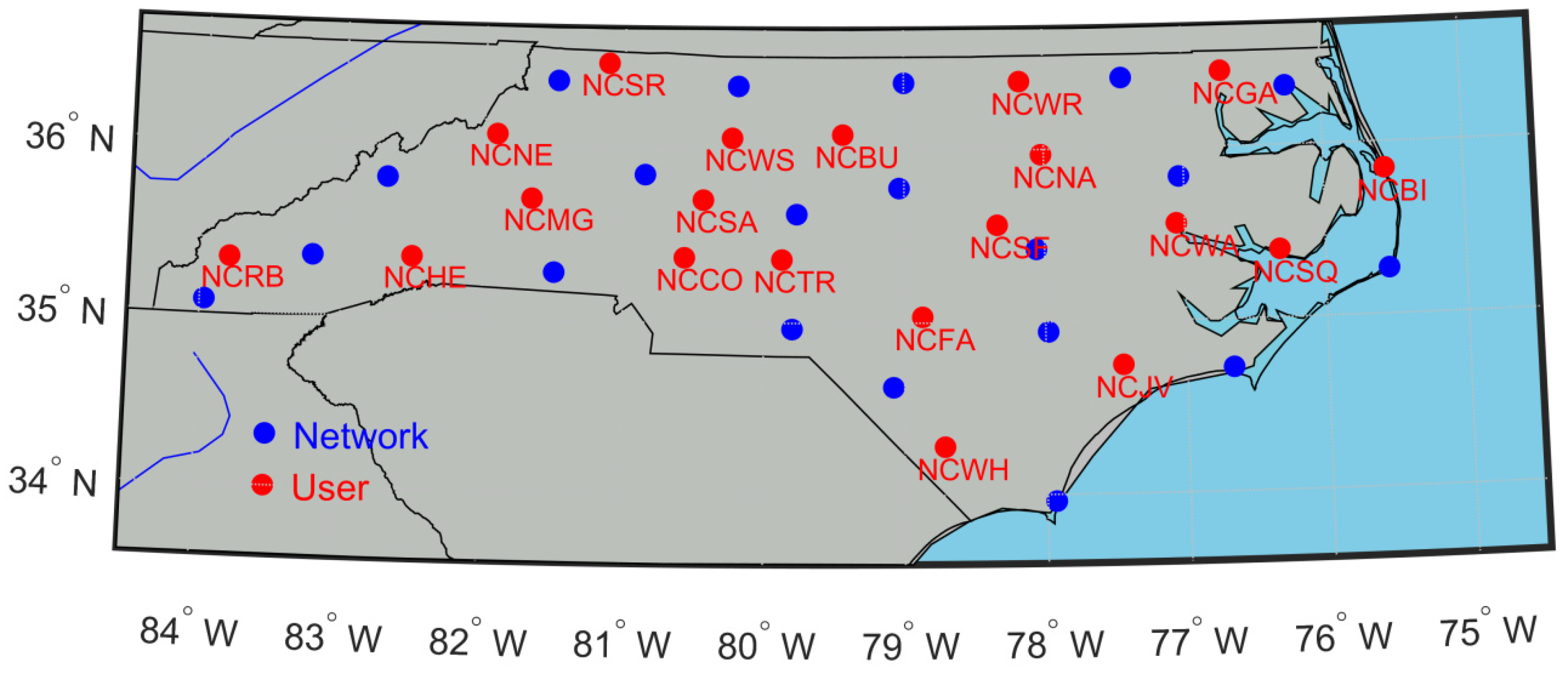
The North Carolina Continuously Operating Reference Station Network is composed of more than $60$ permanent stations, among which $20$ stations regularly distributed over the state were chosen as the reference to provide the satellite clock and phase delay corrections, as well as the tropospheric delay corrections. The average baseline length is about $100\mathrm{km}$. Another $20$ stations within and at the edge of the network are considered as user locations to validate the accuracy of the tropospheric delay correction and the performance of the tropospheric-weighted model. The locations of the reference and user stations can be seen in Figure 1.

The processing strategy options are summarized in

Table 1. Summary of the strategy of data processing for data processing.

Parameter	Strategy and Value
	Network	User
Positioning mode	Fixed	Kinematic/Static
Constellation	GPS	GPS
Frequency	L1 and L2	L1 and L2
Satellite orbits	IGS final	IGS final
Interval	$30\mathrm{s}$	$30\mathrm{s}$
Elevation cutoff angle	$10°$	$10°$
Kalman filter	Forward and backward	Forward
Standard deviation (STD) of phase/code observable	$0.005\mathrm{m}$/$0.5\mathrm{m}$	$0.005\mathrm{m}$/$0.5\mathrm{m}$
Weighting strategy	Elevation dependent	Elevation dependent
Zenith hydrostatic delay	Saastamoinen model	Saastamoinen model
Zenith wet delay	Estimate with the process noise $0.0001{\mathrm{m}}^2/\mathrm{s}$	Estimate with the process noise $0.0001{\mathrm{m}}^2/\mathrm{s}$
Slant ionospheric delay	Epoch independent	Epoch independent
Receiver clock offset	Epoch independent	Epoch independent
Satellite clock offset	Epoch independent	/
Receiver phase delay	Constant	Constant
Satellite phase delay	Constant	/
Ambiguity	Constant	Constant
Integer ambiguity resolution	Partial (with the success rate criterion $0.999$)	Partial (with the success rate criterion $0.999$)

. One can see that the IGS final orbit products are chosen as the precise satellite ephemeris in considering their highly precise satellite positions. The purpose is to reduce the satellite orbit errors to the maximum extent, since this study mainly focuses on the tropospheric delay corrections. Therefore, we intended to eliminate any other error sources and draw confidential conclusions without irrelevant influences. The real-time users do not need to worry about the time limit of the IGS final products since numerous research works have studied real-time and ultra-orbit products [32,33].

The data processing strategies for both network and user are quite similar. As demonstrated in the previous section, the satellite clock offset and satellite phase delay parameters are not estimated on the user side for the purpose of avoiding rank deficiency problems, and thus, these two types of unknowns are not applicable on the user side. Note that partial integer ambiguity resolution with a success rate criterion $0.999$ is implemented in the data processing, which means that only a subset of ambiguities is fixed to integer values such that a user-defined success rate criterion is met, rather than fixing all ambiguities.

3.1. Accuracy of the Tropospheric Corrections

Since the hydrostatic delays at both network and user stations have been corrected by the Saastamoinen model in preprocessing, only the wet delays are generated through the Kriging from the network at each epoch and provided to the user. Meanwhile, the zenith wet delays are also estimated at the user stations using the standard PPP-RTK model of (3) and regarded as the true value to verify the accuracy of tropospheric corrections.

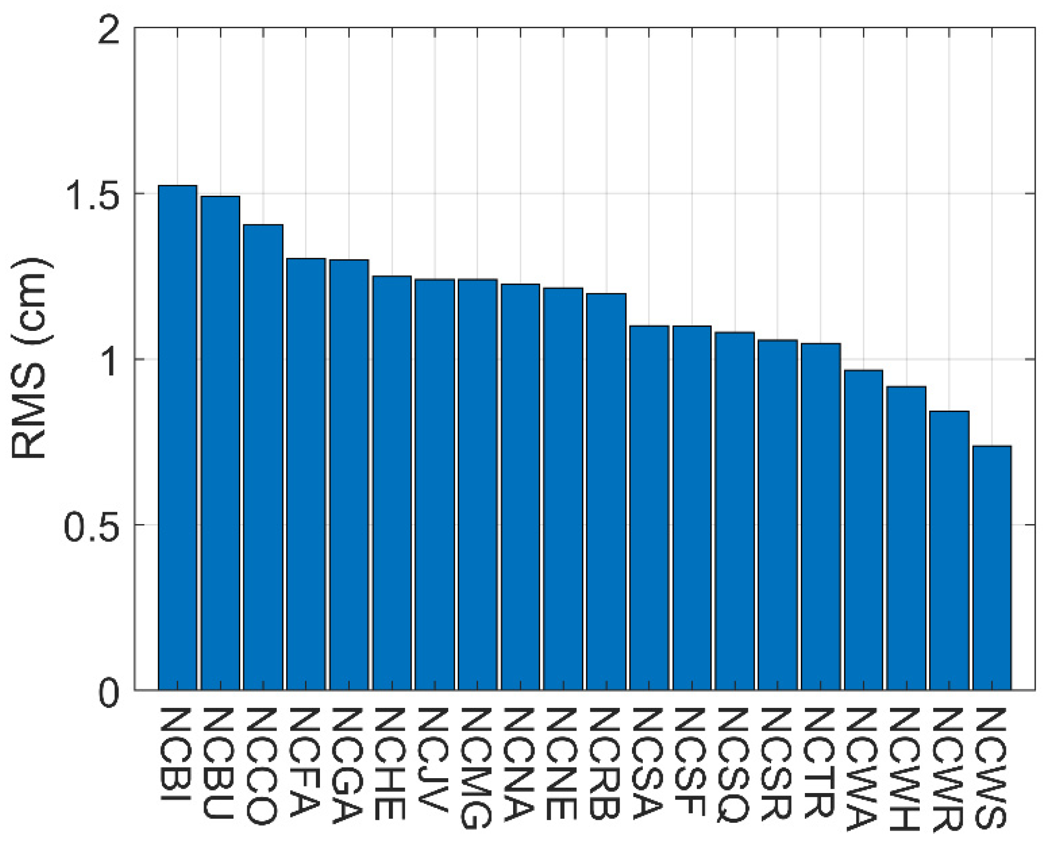
The Root Mean Square (RMS) errors of the tropospheric corrections at each user station after convergence are presented in Figure 2, which vary from $0.8$ to $1.5\mathrm{cm}$. It is worth mentioning that the quality of the corrections does not relate to the user locations, which means that $1$ cm-level accuracy can be obtained so long as the users are in the network.

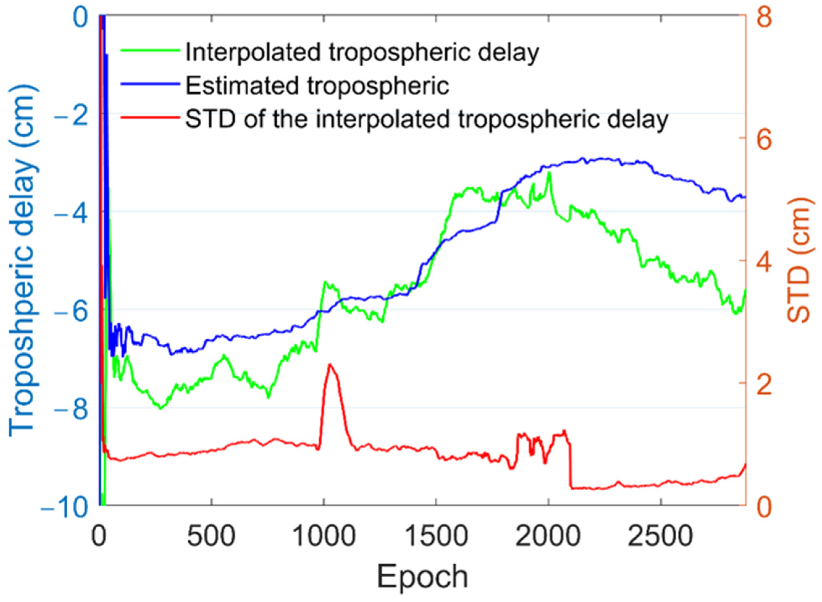
The time series of the interpolated and estimated tropospheric delay of the station NCWA is presented in Figure 3. One can see that the two types of tropospheric delays have a similar trend. However, the estimated solutions are smoother because they are tightly constrained in the filter processing, which means the interpolation strategy can still be further improved, e.g., by applying a filtering method to remove the turbulence between two epochs. It is worth noting that the values of the estimated tropospheric delay are negative. As is well known, this is because the hydrostatic part of the tropospheric delay is usually compensated by an empirical model, e.g., the Saastamoinen model used in this study [34]; the residuals caused by the empirical model would be lumped into the wet delay. With the overestimating of the hydrostatic delay, the extra hydrostatic delay is taken into account in the wet delay and leads to negative values. Although the negative wet delay does not have a physical sense, considering that the hydrostatic delay is two orders of magnitude larger than that of the wet delay, the combined delay is still positive.

The STDs provided by the Kriging vary over time since they depend not only on the distances between the user and network stations but also the variograms, which illustrate the variations of the known points. As can be seen in Figure 3, the STDs can nearly represent the displacement between the estimated and interpolated tropospheric delays. For instance, the STDs of the predicted tropospheric delay at the beginning of the data processing are higher due to the fact that the tropospheric delay estimations at the network have not converged, indicating less precise tropospheric delay corrections. The jump of STD around the $1000\mathrm{th}$ epoch is because of the unusual tropospheric estimations at one reference station, which causes a significant change of the variogram. Users have other options to represent the uncertainty of the interpolated corrections, for instance, a small value for normal weather conditions and a big value for a weather event.

3.2. Accuracy of the Kinematic Positioning

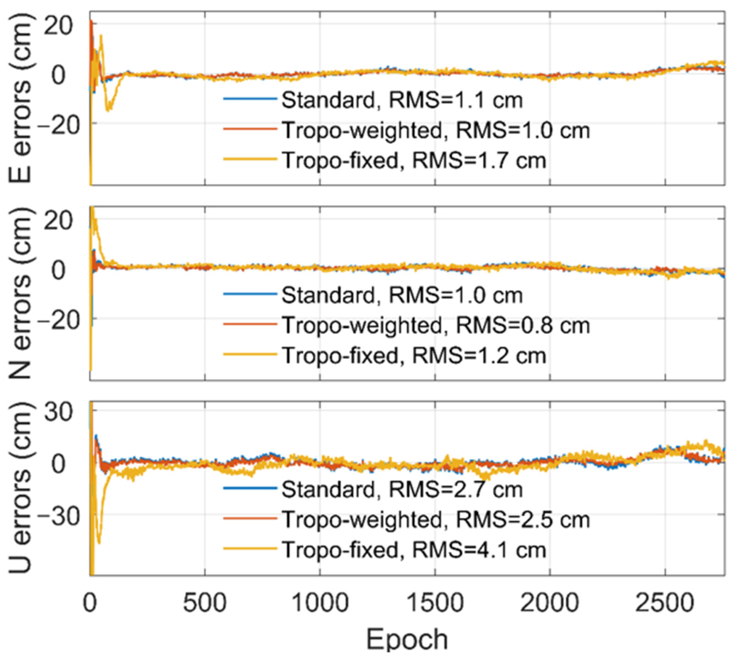
The $20$ user station dataset has been processed in kinematic mode to assess the performance offered by the tropospheric-weighted model. As can be seen in

Table 2. Cases of the PPP-RTK positioning modes.

		Integer Ambiguity Resolution
		Float	Fixed
PPP-RTK model	Standard	☑	☑
	Tropospheric-weighted	☑	☑
	Tropospheric-fixed	☑	☑

, six cases of ambiguity-float and -fixed solution of the standard PPP-RTK model as well as the tropospheric-weighted model are involved in the data processing of the accuracy experiment and the following convergence experiment. In addition, the tropospheric-fixed model for which the interpolated tropospheric delays are considered as the deterministic corrections rather than stochastic is also applied in the data processing to illustrate the advantage of taking into account the uncertainty of the interpolated corrections.

Figure 4 presents the ambiguity-float positioning errors of the user stations NCWA under three different models. One can see that the time series of the standard model is aligned to that of the tropospheric-weighted model, while the errors of the tropospheric-fixed model are distinguishable, especially for the up component. This is because the unavoidable errors of the interpolated corrections must influence the positioning solutions. Furthermore, the tropospheric delay and vertical direction are highly correlated. An increased tropospheric-fixed positioning error can be seen in up components.

The ambiguity-fixed positioning solutions of the same station are shown in Figure 5, in which the performances of three models are all improved as compared to those of the ambiguity-float solutions. However, the tropospheric-fixed solution requires more time to achieve the same accuracy level as the standard and tropospheric-weighted model because the imperfect corrections may cause harm to integer ambiguity resolution, and further affect the positioning solutions.

Statistics of the RMS errors of the different positioning models are presented in Figure 4 and Figure 5. Note that the statistics are calculated from the $4\mathrm{th}$ hour to the end, during which positioning solutions are already fully converged. The tropospheric-fixed model yields good performances, but they are still worse than the standard and tropospheric-weighted model. This is because the tropospheric-fixed model is mostly implemented in the two-step satellite orbit determination for which the tropospheric delays are estimated accurately by GPS and then used for determining other orbits of navigation satellite systems. In this case, the tropospheric effects are common to all constellations because they are the delays of one station.

As for the positioning, however, the user receivers may not be even close to the reference, and thus, interpolating errors are unavoidable in the troposphere corrections. If these errors are not carefully addressed, the positioning solutions would be influenced, especially for the up component due to the high correlation. This phenomenon can be seen in Figure 4 for the ambiguity-float solutions and Figure 5 for the ambiguity-fixed solutions. It is worth noting that the E and N components of the tropospheric-fixed model have the same accuracy as the standard model for the ambiguity-fixed solutions, which means that fixing ambiguities can eliminate the positioning errors caused by the inaccurate troposphere corrections to some extent.

Table 3. Average RMS of the $3\mathrm{D}$ positioning errors of ambiguity-float and -fixed solution at the user stations in the standard, tropospheric-weighted, and tropospheric-fixed model.

	Ambiguity-Float Positioning Solution (m)			Ambiguity-Fixed Positioning Solution (m)
	Standard	Tropo-Weighted	Tropo-Fixed	Standard	Tropo-Weighted	Tropo-Fixed
Average	0.031	0.028	0.034	0.027	0.023	0.026

presents the average RMS of the $3\mathrm{D}$ positioning errors of ambiguity-float and -fixed solution at $20$ user stations in the use of standard, tropospheric-weighted, and tropospheric-fixed model. Again, the statistics are calculated from the $4\mathrm{th}$ hour to the end. One can see an insignificant improvement of the tropospheric-weighted model as compared to the standard because the positioning results of the standard approach are already accurate enough for both the ambiguity-float and -fixed solution. The tropospheric pseudo-observable could hardly augment the strength of the underlying PPP-RTK model after convergence.

The gains for positioning with the tropospheric-weighted model are about $9.6\%$ (ambiguity-float) from $3.1$ to $2.8\mathrm{cm}$ and $14.8\%$ (ambiguity-fixed) from $2.7$ to $2.3\mathrm{cm}$. The accuracy of the ambiguity-fixed positioning solutions are close to that of the ambiguity-float solutions because the benefits of fixing integer ambiguities are marginal after convergence.

As for the tropospheric-fixed model, the accuracy of the ambiguity-float solutions degrades, from $3.1\mathrm{cm}$ to $3.4\mathrm{cm}$ on average for the standard model due to the errors of the interpolated corrections. The ambiguity-fixed solution of the tropospheric-fixed model with an average of $2.6\mathrm{cm}$ accuracy is slightly better than that of the standard model with $2.7\mathrm{cm}$. However, this might be completely random since there is only a $1\mathrm{mm}$ improvement in a only a few solutions, and for the ambiguity-fixed solutions of the tropospheric-fixed model, only half of the stations are improved compared to the standard model. Therefore, it is not evident that the tropospheric-fixed model is better than the standard.

3.3. Convergence Time of the Kinematic Positioning

Except for positioning accuracy, the convergence time is another factor that users may be interested in. In order to quantify the benefits of using tropospheric corrections towards the convergence time, the data processing of the standard and tropospheric-weighted model are re-initialized for all user stations at each from $1\mathrm{st}$ to $20\mathrm{th}$ h, which means that for each user station, we can have $20$ convergence time solutions. The criterion for convergence is the last time the positioning errors, e.g., $3\mathrm{D}$, horizontal, and up component, decrease to the $10\mathrm{cm}$ level. Only two hours of data from the start are processed because the positioning solution must have converged within two hours. Note that only the standard and tropospheric-weighted model are involved in the experiment of the convergence time because the performance of the tropospheric-fixed is not superior to that of the standard model.

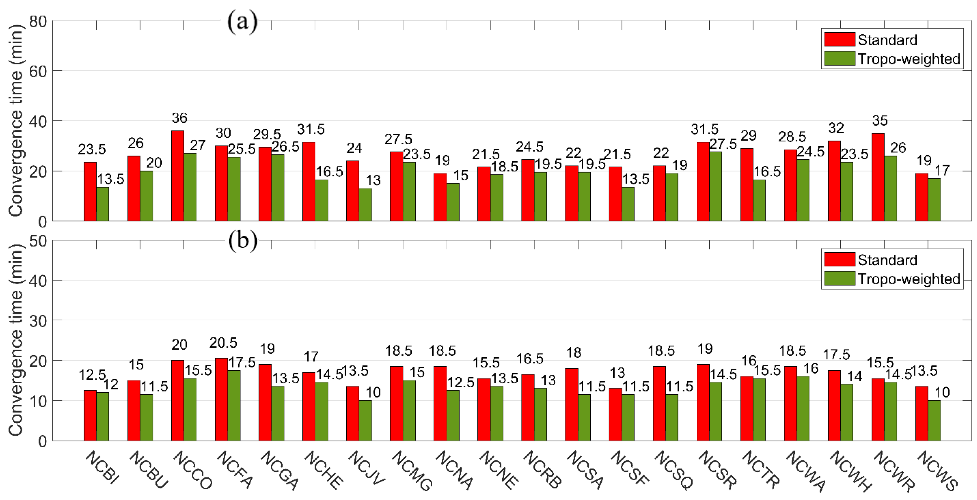
Figure 6 presents the convergence time of the $3\mathrm{D}$ ambiguity-float and -fixed positioning solutions with a $90\%$ probability, which means that with $90\%$ probability, one can obtain a better result than the values shown in the figure. The reason for not taking into account all convergence solutions is to eliminate the effects of the unusual error behavior in data processing, since there are unpredictable model errors that might be involved in the data. One can see that for most user stations in the top panel of Figure 6, reducing convergence times of $4$ to $10$ min appears in the implementation of the tropospheric-weighted model for kinematic data processing. This is because the tropospheric pseudo observable can, on the one hand, strengthen the underlying model so that the impact of the biases can be partly eliminated, and on the other hand, the Kriging has assured a certain level of corrections accuracy. Overall, the tropospheric-weighted model can shorten the convergence time to reach a $10\mathrm{cm}$ $3\mathrm{D}$ positioning accuracy based on the ambiguity-float solution by $4.5\min$ from $48$ to $43.5\min$ with $90\%$ probability.

The convergence times of the ambiguity fixed solutions, as shown in the bottom panel of Figure 6, are significantly shortened for both standard and tropospheric-weighted models compared to the top panel, the ambiguity-float solutions. This is because after fixing the ambiguity, the positioning model strength would be enhanced since extra pseudo-observations from fixing ambiguity are added to the functional model. In addition, the horizontal component is strongly correlated with the ambiguities, and therefore, once the ambiguities are successfully fixed, the accuracy of the positioning results will be significantly improved. Besides, the dispersion of the convergence times of fixed ambiguity positioning solution at different user stations is small, so that one can expect a $25\min$ observation session length if the receiver is in the network. The contribution of the external tropospheric corrections for the ambiguity fixed solutions is similar to the ambiguity-float solutions since the improvements in terms of convergence time between the standard and tropospheric-weighted model remain in the same scale. This is because the strengthened functional model by the troposphere pseudo observable can also contribute to the fast and successful integer ambiguity resolution, especially when the geometry is not good enough, e.g., only a few satellites can be observed. For the ambiguity-fixed solutions, an improvement of $5.5\min$ is achieved by the tropospheric-weighted model from $27$ to $21.5\min$.

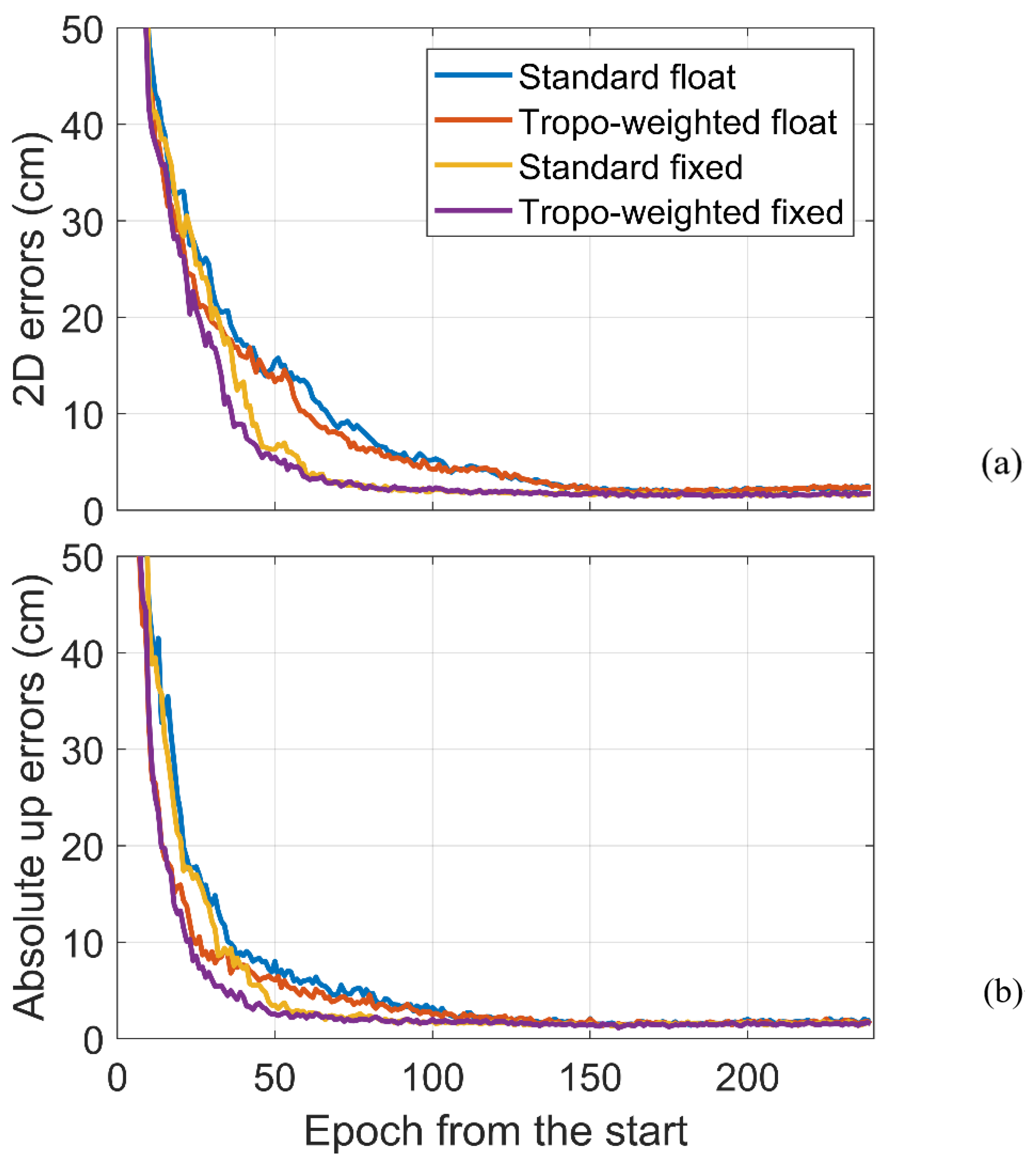
Figure 7 shows the horizontal and absolute up component positioning errors of each positioning mode at each epoch with a $90\%$ probability. Note that the $x$-axis is the epoch from the start of data processing so that the characteristics of all processes of $20$ user stations can be visually displayed and compared. One can see that at the beginning of the top plot, the positioning errors of the four positioning cases are not distinguishable. However, on the $0.2$ to $0.3\mathrm{m}$ positioning error level, the performances of the tropospheric-weighted ambiguity float and fixed solutions are better than those of the standard model. The partial integer ambiguity resolution is implemented in the data processing, which means only a subset of ambiguities with highly precise estimates can be fixed into integer values rather than whole ambiguities. Therefore, ambiguity-float and -fixed solutions are relatively close together for both the tropospheric-weighted and standard model since not too many ambiguities have been fixed at the beginning of data processing. Meanwhile, the tropospheric-weighted model is stronger with the external pseudo-observable, which leads to an obvious error decrease at this scale as compared to the standard model.

With the accumulation of the observations, the positioning errors of the ambiguity-fixed solutions are quickly reduced, which clearly benefits from the large number of fixed ambiguities. In this case, the ambiguity-fixed solutions spend less time to achieve a certain accuracy level (e.g., $10\mathrm{cm}$ and $5\mathrm{cm}$) compared to the ambiguity-float solutions. Finally, after a long convergence period, the ambiguity-float and -fixed solutions obtain almost the same accuracy level because the ambiguity float positioning models have been strong enough. This also explains the insignificant improvement of the tropospheric-weighted model for the kinematic positioning experiment. In addition, the benefits of the tropospheric-weighted model towards reducing the positioning error can still be seen at the $10\mathrm{cm}$ and $5\mathrm{cm}$ levels.

The patterns of the absolute up positioning errors, as can be seen in the bottom plot of Figure 7, are not the same as the horizontal component. One can see that the differences between float and fixed solutions for both the tropospheric-weighted and standard model are not significant even at the $10\mathrm{cm}$ level, which means the fixed ambiguities do not contribute much to the vertical accuracy. On the contrary, the horizontal positioning errors of fixed solutions have been dramatically reduced at the same accuracy level. This is because of the correlation between ambiguities and the horizontal component, thereby improving the horizontal accuracy once most ambiguities are successfully fixed. It is well known that the zenith tropospheric delay is one of the main error sources for GNSS to achieve an accurate vertical positioning solution, and thus, the tropospheric delay corrections bring with it improvements in vertical positioning accuracy.

Table 4. Summary of the convergence times to achieve $10\mathrm{cm}$ positioning accuracy of the standard and tropospheric-weighted model with $90\%$ probability in kinematic positioning mode (the unit is minutes).

Component	Ambiguity Resolution	Standard	Tropo-Weighted	Improvement in Minute	Improvement in Percentage
3D	Float	48	43.5	4.5	9.38%
	Fixed	27	21.5	5.5	20.37%
Horizontal	Float	37	32.5	4.5	12.16%
	Fixed	22	18	4	18.18%
Vertical	Float	34	26.5	7.5	22.06%
	Fixed	23.5	17	6.5	27.66%

presents the statistics of the corresponding convergence times to achieve $10\mathrm{cm}$ positioning accuracy for different modes. Note that statistics of each position component are counted individually and based on all processes of $20$ user stations in a manner of $90\%$ probability. It is clear that the fixed solutions of either the tropospheric-weighted or standard model have shorter convergence times compared to the float solutions. Furthermore, reduced convergence times can also be seen for the tropospheric-weighted model for which the $3\mathrm{D}$ positioning is $4.5\min$ for the float solution and $5.5\min$ for the fixed solution. The improvements of the vertical component are $7.5\min$ and $6.5\min$ for the float and fixed solution, which are bigger than those of the horizontal component at $4.5\min$ and $5\min$, respectively.

3.4. Convergence Time of the Static Positioning

Static positioning is also widely used today by companies offering surveying and mapping services. It assumes that the receiver is stationary rather than in motion, and thus, its positioning model is stronger than that of the kinematic since the coordinates remain constant over time. The convergence times of the static positioning, as shown in the top panel of Figure 8 with the float solution and in the bottom panel with the fixed solution, have better performances than those of kinematic positioning solutions in Figure 6.

An improvement of 6 min can be seen for the ambiguity float solution from the standard model with 31.5 min compared to the tropospheric-weighted model with 25.5 min. However, this convergence time is only shortened by $3.5\min$ for the ambiguity-fixed solution because the benefit of the external pseudo-observable is limited due to the increase of the underlying model strength.

The horizontal and up component positioning errors are shown in Figure 9. It can be seen that the standard model achieves practically the same performance at the $10\mathrm{cm}$ level accuracy as the tropospheric-weighted model with the external corrections in horizontal components. There is only a reduction of $2\min$ for the tropospheric-weighted model to achieve $10\mathrm{cm}$ positioning accuracy, as presented in

Table 5. Summary of the convergence times to achieve $10\mathrm{cm}$positioning accuracy of the standard and tropospheric-weighted model with $90\%$ probability in static positioning mode (the unit is minutes; values in brackets denote the convergence times to achieve $5\mathrm{cm}$ positioning accuracy).

Component	Ambiguity Resolution	Standard	Tropo-Weighted	Improvement in Minute	Improvement in Percentage
3D	Float	31.5 (47)	25.5 (41.5)	6 (5.5)	19.05% (11.70%)
	Fixed	18.5 (21.5)	15 (18)	3.5 (3.5)	18.92% (16.28%)
Horizontal	Float	24.5 (39)	22.5 (38)	2 (1)	8.16% (2.56%)
	Fixed	15.5 (19.5)	13.5 (16.5)	2 (3)	12.9% (15.38%)
Vertical	Float	24 (37)	16 (28.5)	8 (8.5)	33.33% (22.97%)
	Fixed	15.5 (20)	12 (16.5)	3.5 (3.5)	22.58% (17.50%)

. This is because, as mentioned before, the contribution of the pseudo-observable on the horizontal component is attenuated as the underlying model becomes strong. However, one can expect larger improvements of the vertical component in the use of the tropospheric-weighted model, which are $8\min$ for the float solution and $3.5\min$ for the fixed solution. Table 5 also gives the convergence times to achieve $5\mathrm{cm}$ level accuracy, for which the improvements of the tropospheric-weighted model are similar to those of the $10\mathrm{cm}$. This confirms the advantage of the tropospheric-weighted model in more accurate positioning solutions.

4. Conclusions and Discussion

In this contribution, instead of compensating the wet delay with deterministic values (the so-called tropospheric-fixed model), we introduce the stochastic properties of the external corrections into the functional positioning model to construct the tropospheric-weighted model. The wet delay corrections are generated by Kriging interpolation, which can also provide proper constraints for interpolated corrections. The RMSs of the tropospheric corrections at $20$ user stations vary from $0.8$ to $1.5\mathrm{cm}$ after convergence when compared to the tropospheric delays independently estimated at the corresponding station, which are accurate enough to be regarded as the pseudo-observable. The Kriging interpolation applied in this study does not consider the time correlation between adjacent corrections since, traditionally, it only considers the spatial correlation of a certain region. However, it is worthwhile to introduce the time-correlation into the tropospheric delay correction generating strategy because it is widely known that the tropospheric delay is highly time-correlated. Therefore, after considering the time correlation, the precision of the tropospheric delay corrections could be further improved.

Then, the dataset is first processed with the kinematic positioning strategy in both ambiguity-float and -fixed positioning solutions. It has been demonstrated that the performance of the tropospheric-fixed model is not better than that of the standard model. As for the tropospheric-weighted model, the results show that the improvement in terms of positioning accuracy is not significant because the positions obtained by the standard model have already been very accurate, and the standard model is strong enough after convergence; thus, the contribution of the tropospheric corrections is limited. One can only see that the improvements of the tropospheric-weighted model are at the millimeter-level for both the ambiguity-float and -fixed solutions.

Then, the tropospheric-weighted model is evaluated in terms of required time to achieve 10 cm positioning accuracy in kinematic and static positioning strategy separately. Taking into account all the convergence time solutions, $90\%$ of the $3\mathrm{D}$ convergence times of the standard model for the ambiguity-float solution are $48\min$ for the kinematic mode and $31.5\min$ for the static mode, while for the tropospheric-weighted model, they are $43.5\min$ and $25.5\min$, with improvements of $4.5\min$ and $6\min$, respectively.

The tropospheric-weighted model can also benefit from the ambiguity-fixed solution. The tropospheric-weighted model can reduce the convergence times of the ambiguity-fixed solution by $5.5\min$ for the kinematic mode from $27\min$ to $21.5\min$, and by $3.5\min$ for the static mode from $18.5\min$ to $15\min$.

Compared to the horizontal component, the shortened convergence times on the vertical component for both kinematic and static mode are more significant, which can be understood as the tropospheric delay being highly correlated with vertical position. Results of the experiment with $5\mathrm{cm}$ convergence threshold indicate that the tropospheric-weighted model can still work well in more accurate positioning solutions.

It is worth noting that the tropospheric delay correction generating method can be implemented in both small and large networks. This is because, as demonstrated previously, that the Kriging interpolation depends upon the distances between the unknown points and all available measurements, and the variation information of the interpolated values can also be provided. In other words, when the experiment region is small, the corrections will be precisely generated because of the correlation of the neutral atmosphere; meanwhile, the standard deviations of these corrections are at a relatively low level. On the contrary, when the experiment region is large, the corrections may not be precisely generated because the correlation of the neutral atmosphere is not obvious; at the same time, the standard deviations of the tropospheric delay correction must be at a relatively high level because the weights of the Kriging corrections partly depend on the distance. Besides, this method is independent of the satellite positioning data processing, which means that regardless of whether the receiver is the single, dual, or triple frequency, this proposed method can generate the tropospheric delay corrections.