Technical Note

Performance of SMAP and SMOS Salinity Products under Tropical Cyclones in the Bay of Bengal

1
College of Electronic and Information Engineering, Guangdong Ocean University, Zhanjiang 524088, China
2
Southern Marine Science and Engineering Guangdong Laboratory (Zhuhai), Zhuhai 519000, China
*
Author to whom correspondence should be addressed.
Remote Sens. 2022, 14(15), 3733; https://doi.org/10.3390/rs14153733
Submission received: 17 June 2022 / Revised: 27 July 2022 / Accepted: 2 August 2022 / Published: 4 August 2022

Abstract

:
To compare the accuracy of satellite salinity data of level-3 Soil Moisture Active Passive V4.0 (SSMAP) and debiased v5 CATDS level-3 Soil Moisture and Ocean Salinity (SSMOS) before and after tropical cyclones (TCs) in the Bay of Bengal (BoB), this study used the sea surface salinity of Argo (SArgo) to assess SSMAP and SSMOS before and after the passage of 10 TCs from 2015 to 2019. The results indicate that the SSMAP and SSMOS agreed well with SArgo before and after 10 TCs. It can be seen that the correlation between SSMAP and SArgo (before TCs: SSMAP = 0.95SArgo + 1.52, R2 = 0.83; after TCs: SSMAP = 0.87SArgo + 4.34, R2 = 0.79) was obviously higher than that of SSMOS and SArgo (before TCs: SSMOS = 0.68SArgo + 10.38, R2 = 0.62; after TCs: SSMOS = 0.88SArgo + 3.98, R2 = 0.58). The root mean square error (RMSE) was also significantly higher between SSMOS and SArgo (before TCs: 0.84 psu; after TCs: 0.78 psu) than between SSMAP and SArgo (before TCs: 0.58 psu; after TCs: 0.47 psu). In addition, this study compared SSMAP and SSMOS during two TCs that swept in nearshore and offshore waters, and the results show good agreement between SSMAP and SArgo in the nearshore and offshore waters of BoB. In the BoB, both SSMAP and SSMOS can retrieve sea surface salinity well, and SSMAP is overall better than SSMOS, but the SMOS salinity product can fill the gap of SMAP from 2010 to 2015.

1. Introduction

The Bay of Bengal (BoB), located in the northern part of the East Indian Ocean, is a typical sea area affected by South Asian monsoons. The South Asian summer monsoon brings abundant precipitation to the BoB, which greatly exceeds the evaporation capacity. Coupled with the injection of many runoffs around the bay, the input of a large amount of freshwater makes the BoB have the lowest salinity in the Indian Ocean, which induces a thick barrier layer. The changes in upper salinity not only affect the current circulation in the bay [1], but also play an important role in modulating the ocean’s Response to Tropical Cyclones (TCs) owing to the formation of the thick barrier layer [2,3].
Sea surface salinity is mainly detected by in situ observations (cruise, Argo, surface drifters, and buoys) and satellite measurements. Satellites (Aquarius, Soil Moisture and Ocean Salinity (SMOS), Soil Moisture Active Passive (SMAP)) provide a unique opportunity to produce synoptic maps of BoB salinity. SMOS V2.0 only captures the seasonal evolution of sea surface salinity in the northern BoB [2], but the Aquarius salinity product accurately captures seasonal signals in the entire basin [4]. The updated CATDS V4.0 level-3 salinity product from SMOS has much better performance [5]. The salinity product from SMOS now performs equivalently to Aquarius, but is slightly inferior to SMAP in the BoB [5]. SMOS, which was launched in 2009, has an average resolution of close to 43 km. SMAP, which was launched in 2015, provides retrieved sea surface salinity data with a spatial resolution of 40 km. SMAP has lighter land contamination and is less affected by radio frequency interference than SMOS [6]. Aquarius was launched in 2011 but was terminated in 2015 owing to an unrecoverable hardware failure. Moreover, Aquarius only provides salinity products with an effective resolution of ~150 km.
The BoB experiences intense TCs during the pre-monsoon (April–May) and post-monsoon (October–November) months. The thick barrier layer can affect the intensity of TCs and biological productivity by inhibiting vertical mixing [7,8,9]. Strong TC-induced mixing and upwelling cause a significant increase in sea surface salinity in the open ocean [10,11,12,13]. In the BoB, TC Vardah increased sea surface salinity up to 1.5 psu based on SMAP salinity observations [14]. The high winds of TCs can affect surface roughness, resulting in variations in satellite-observed brightness temperatures [15,16], which can affect salinity retrieval.
There are many studies assessing the salinity accuracy of SMAP, Aquarius, and SMOS in the oceans, but only a few studies have been designed to assess the accuracy of satellite salinity products under the effects of TCs. Xu et al. reported that the 8-day SMAP salinity product agreed well with the Argo salinity product before and after 25 TCs in the BoB [17]. However, the SMAP product only provides salinity data from 2015 to the present. The SMOS data cover a longer period than SMAP data, since 2010. In addition, the SMOS satellite data have recently been upgraded to version 5.0, which is greatly improved compared to the previous version. In this study, we compared the debiased v5 CATDS level-3 SMOS and level-3 SMAP v4.0 salinity products to the Argo measurement before and after 10 TCs to assess the data accuracy of the two satellites.

2. Data and Methods

The spatial resolution of the 8-day Level 3 SMAP ocean surface salinity product version 4.0 is approximately 70 km. The 70 km fields have significantly less noise than the 40 km data. The SMAP website (http://www.remss.com/missions/smap/, accessed on 1 October 2021) provides data with a geospatial resolution of 0.25° × 0.25° since 1 April 2015 [18]. The SMOS L3 product is generated by CATDS CEC LOCEAN debiased V5.0, which is corrected from systematic biases using an improved de-biasing technique [19]. The effective resolution of SMOS salinity data is approximately 43 km. The SMOS website (https://www.catds.fr/Products/Available-products-from-CEC-OS/CEC-Locean-L3-Debiased-v5/, accessed on 1 October 2021) provides 9-day averaged SOMS data with a geospatial resolution of 0.25° × 0.25° since 16 January 2010. The 6-hourly track data and maximum 10 m-sustained wind speed of TCs were obtained from the Regional Specialized Meteorological Centre (RSMC) of the India Meteorological Department (http://www.rsmcnewdelhi.imd.gov.in/, accessed on 1 October 2021). Ten TCs were chosen from April 2015 to December 2019, which were observed by no fewer than 6 Argo floats within 2° of the TC tracks. The tracks and basic information of these 10 TCs are shown in Figure 1 and Table 1, respectively.
The International Argo Program (www.argodatamgt.org/, accessed on 1 October 2021) provides salinity data from Argo floats. In this study, we divided Argo salinity (SArgo), SMAP salinity (SSMAP), and SMOS salinity (SSMOS) into two parts: ~8 days before and ~8 days after 10 TCs, within 2° of the TC’s center. For example, TC Roanu swept the BoB during 17–22 May 2016. The first part included Argo floats 8 days before 17 May within 2° of the TC center, and the second part included Argo floats 8 days after 16 May within 2° of the TC center. We chose the ~8-day average SSMAP and SSMOS before 17 May and after 16 May. A matched pair of in situ Argo and SMOS and SMAP observations was selected when Argo floats were within +/−8 days of satellite observations and when the satellite observations were within 27.75 km of the floats. We chose 119 Argo floats ~8 days before and 121 Argo floats ~8 days after the 10 TCs. The positions of all selected Argo floats are shown in Figure 1. The shallowest salinity (<10 m) from Argo floats was selected to represent surface salinity. The average depth of SArgo data was 4.05 ± 2.15 m. The matched pairs were defined as follows:
ΔS = Ssatellite data (position of Argo float) − SArgo (position of Argo float)
In this study, we calculated the mean, standard deviation (STD), linear correlation coefficient (R), bias ( 1 N i = 1 N ( S SMAP   or   SMOS ( i ) S A r g o ( i ) ) ), and root mean square error (RMSE; 1 N i = 1 N ( S SMAP   or   SMOS ( i ) S A r g o ( i ) ) 2 ) to evaluate the performance of SMAP and SMOS salinity products during the passage of 10 TCs in the BoB.

3. Results and Discussion

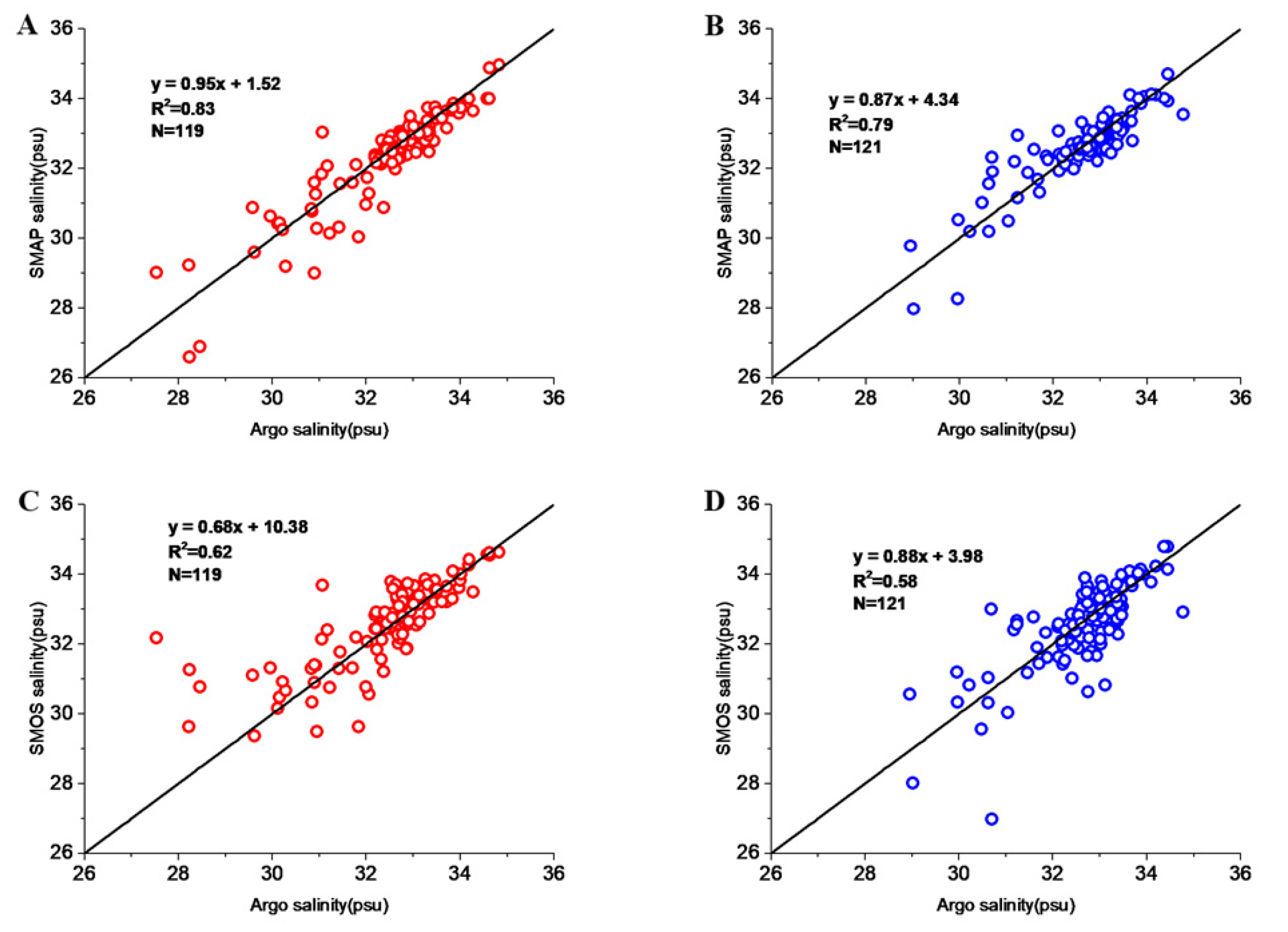
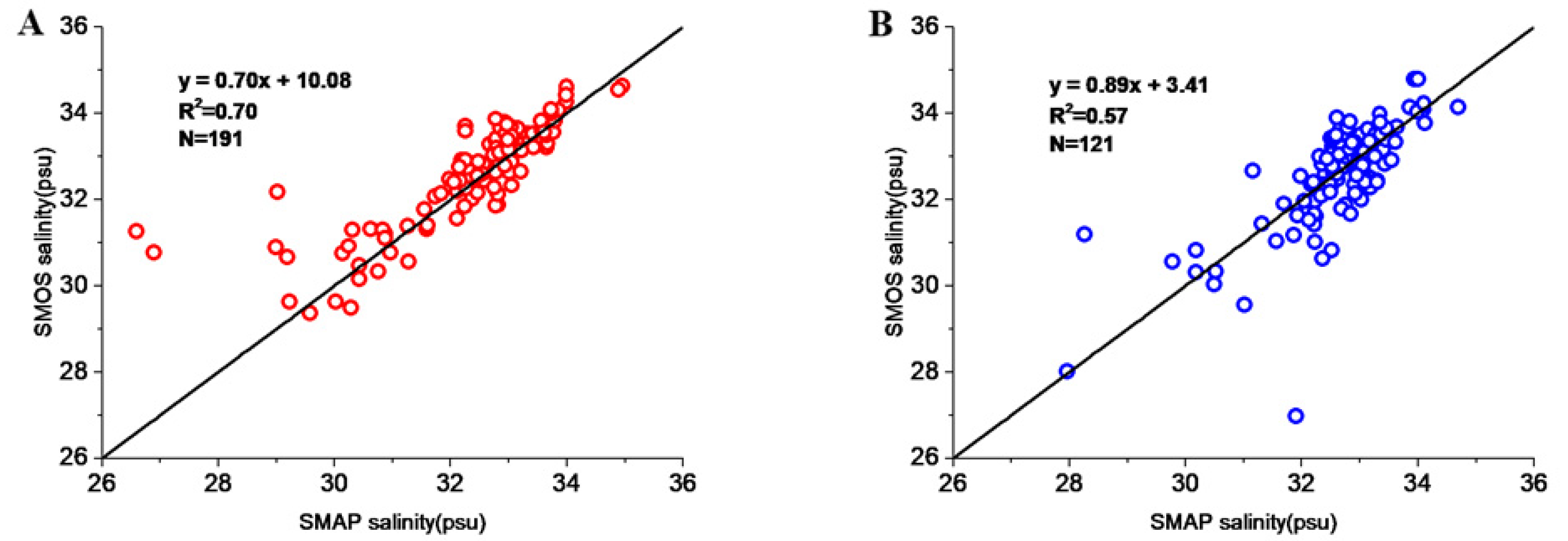
3.1. SMOS and SMAP Product Validation with Argo Salinity

In this study, the salinity product was divided into two groups: before TCs and after TCs. The differences between the satellite salinity data and the in situ Argo data were analyzed to verify the performance of the two satellites before and after 10 TCs. Figure 2 shows the correlations between SSMAP, SSMOS, and SArgo before and after 10 TCs. Before the TCs, the correlations were: SSMAP = 0.95SArgo + 1.52 (R2 = 0.83, N = 119) and SSMOS = 0.68SArgo + 10.38 (R2 = 0.62, N = 121). After the passage of 10 TCs, the correlations were: SSMAP = 0.87SArgo + 4.34 (R2 = 0.79, N = 119) and SSMOS = 0.88SArgo + 3.98 (R2 = 0.58, N = 121). The results indicate that the SMAP and SMOS salinity products agreed well with the in situ Argo salinity product (R2 > 0.5) and the retrieved salinity from SMAP was better than that of SMOS. After the 10 TCs, the coefficient of determination (R2) declined slightly, so the passage of the TCs affected the retrieval accuracy of the two satellites.
Table 1 shows the coefficient of determination between SSMAP, SSMOS, and SArgo for 10 TCs. The results show that the SMAP product could well retrieve sea surface salinity under the influence of most TCs. Among them, only after very severe cyclonic storm (VSCS) Gaja, SMAP salinity did not agree well with the in situ Argo salinity (R2 ≤ 0.3). The coefficient of determination for SMOS salinity after VSCS Vardah, Cyclonic Storm Maarutha, and Severe Cyclonic Storm (SCS) Mora was very low (R2 ≤ 0.3). These results indicate that SMOS is inferior to SMAP. In this study, under the influence of two severe tropical storms, VSCS Vardah and VSCS Gaja, the coefficient of determination between SSMAP and SArgo dropped significantly from 0.90 before Vardah to 0.53 after Vardah, and dropped from 0.60 before Vardah to 0.15 after Gaja. In addition, the salinity data of the two satellites before TCs are highly correlated: SSMOS = 0.70SSMAP + 10.08 (R2 = 0.70) (Figure 3). The passage of the 10 TCs caused a significant decrease in the correlation between the two satellites (SSMOS = 0.89SSMAP + 3.41, R2 = 0.57).
Table 2 shows the mean, bias, and root mean square error (RMSE) between satellite products and SArgo before and after 10 TCs. The results show that the mean SSMAP before the 10 TCs was 32.33 ± 1.39 psu, which is smaller than the mean SArgo (32.44 ± 1.34 psu). This result is consistent with a previous study in the BoB using the same SMAP and Argo salinity data [17]. However, the mean SSMOS (32.60 ± 1.16 psu) is larger than the mean SArgo. Due to the lack of Argo surface data, most of the Argo salinity data were acquired at ~5 m below the sea surface. The average depth of the Argo data in this study was 4.05 ± 2.15 m, while the satellite measures sea surface salinity shallower than 2 cm. Hence, the value of the in situ Argo salinity data should be higher than the remote sensing observation data [17,20]. In order to show the contrast between the surface and the shallowest depth of Argo, owing to the absence of surface salinity from Argo, we used the observations at 1 and 5 m of the RAMA moored buoy at 15°N, 90°E 8 days before and after TCs Kyant, Roanu, and Vardah. The results indicate that salinity before and after these TCs was lower at 1 m than at 5 m, and the difference between the two depths decreased from 0.026–0.053 psu before to 0.007–0.009 psu after the TCs.
Due to a large amount of runoff and rainfall in the BoB, severe salinity stratification forms on the surface, so surface salinity changes are very drastic [2,3]. TCs can cause intense mixing during their passage, which can break the surface salinity stratification and make the upper seawater homogenized [7,21,22]. The difference between 1 and 5 m decreased to 0.007–0.009 psu after TCs also identified this phenomenon. Owing to the homogenization of upper surface salinity, the observed mean SArgo (32.65 ± 1.03 psu) is very close to the mean SSMAP (32.64 ± 1.00 psu) after the passage of TCs (Table 2). Bias and RMSE between SSMAP and SArgo before the 10 TCs were −0.11 psu and 0.58 psu, respectively, which are smaller than the values between SSMOS and SArgo (0.16 psu and 0.84 psu). After the passage of 10 TCs, the negative bias between SSMOS and SArgo was −0.06 psu, which is higher than the value between SSMAP and SArgo (−0.01 psu); the RMSE between SSMOS and SArgo (0.78 psu) is also significantly higher than that between SSMAP and SArgo (0.47 psu). In this study, the updated SMAP V4.0 data at a spatial resolution of 70 km are smoother on the spatial structures, and the random noise is reduced by approximately 60% compared to the previous version, which is recommended for use in oceanographic applications [23]. This is probably the reason for the lower RMSE values of SMAP than SMOS.
Comparing the difference between SSMAP and SSMOS, it is found that the mean SSMAP before the TCs was 32.33 ± 1.39 psu, which is smaller than that of SSMOS (32.60 ± 1.16 psu). After the TCs passed, the mean SSMAP increased to 32.64 ± 1.00 psu, but the mean SSMOS decreased to 32.59 ± 1.18 psu. Under the influence of the TCs, the intense mixing and upwelling brought deeper and saltier waters to the surface [24,25,26], resulting in an increase in sea surface salinity in a large area in the BoB. The trend of mean SSMAP was consistent with the change of in situ Argo observations, which was 32.44 ± 1.34 psu before TCs and increased to 32.65 ± 1.03 psu after TCs. Therefore, SSMAP better captured the changes in sea surface salinity before and after 10 TCs in the BoB.
Figure 4 shows the correlations between SSMAP, SSMOS, and SArgo after the passage of 10 TCs on the left and right sides of their tracks. The results indicate that the correlations on the left side (R2 = 0.83, SSMAP vs. SArgo; 0.68, SSMOS vs. SArgo) are better than those on the right side (R2 = 0.77, SSMAP vs. SArgo; 0.55, SSMOS vs. SArgo). It is well known that in the Northern Hemisphere, TC-induced cooling is typically more pronounced on the right side of TC tracks [27,28]. This is because clockwise inertial currents are accelerated on the right side due to the rotation of the wind stress vector [29]. This amplifies entrainment and increases mixed layer stirring, which induces serious salinity variability on the right side. In addition, the right-front quadrant also has the highest waves [30]. In these situations, the retrieved salinity from SMAP and SMOS is much better on the left side of the TC track than on the right side, and the mechanism needs to be further studied.
Bao et al. compared the satellite SSS products (SMOS and SMAP) globally, and the results were somewhat similar to this study [31]. They found that SMOS and SMAP agreed well with in situ data in the open ocean between 40°S and 40°N. SMAP data were more highly correlated with TAO buoys (1 m) than SMOS data in the tropical Pacific, and the RMSE of SMOS and SMAP was 0.211 and 0.233 psu, respectively, which are smaller than the values in our study [31]. The higher RMSE values were probably due to the use of Argo data in regions with strong near-surface stratification or near river outflows [31,32]. On the other hand, Figure 2 shows a better correlation between satellite data (SMAP and SMOS) and Argo data at middle salinity (32–35 psu) than in fresher water (<32 psu). TCs bring heavy rain before and after their passage, and the SSS decreases and becomes fresher in some areas [33]. There may explain the high RMSE values of 0.47–0.84 psu. Moreover, strong TCs induce intense mixing, advection, and upwelling, which lead to strong small-scale SSS variations. Hence, when evaluating the satellite SSS products before and after TCs, the rich precipitation or strong small-scale SSS variations were found to have a potential influence on the spatial representation errors [34].
The reasons for the variations in the coefficient of determination and RMSE are complicated. Sea surface roughness increases due to strong winds when TCs are passing, and the coverage area of whitecaps and foam increases, which will increase the brightness temperature observed by microwave radiometers [15,16,35,36]. The residual roughness can be observed several days after a TC passes, but the clear impact on the brightness is during its passage when winds are still above 34 kts (17.5 m/s). It should be noted that the satellite products filter the salinity under high wind. For SMAP, salinity observations are filtered out in the L3 time average when wind speed exceeds 15 m/s. In the SMOS version 5 product, they are filtered out when wind speed is higher than 16 m/s.
In addition, there are temporal delays between local (in time) in situ data and 8- to 9-day satellite composite co-localized match-up pairs. Moreover, the strong changes in sea surface salinity lessen rather quickly within 5 days after the passage of a TC [12,13]. Therefore, Argo float measurements taken in this period might differ from composite satellite data that include a temporal average over an 8- to 9-day period.
In this study, the coefficient of determination for SMAP and SMOS was high, but the RSME was high. A recent study used a nonlinear empirical method based on random forest to correct the SMOS product, which reduced RMSE significantly and increased the correlation coefficient between in situ and satellite data [37]. This method could help us to correct salinity data in the new version of SMAP or SMOS in the future.

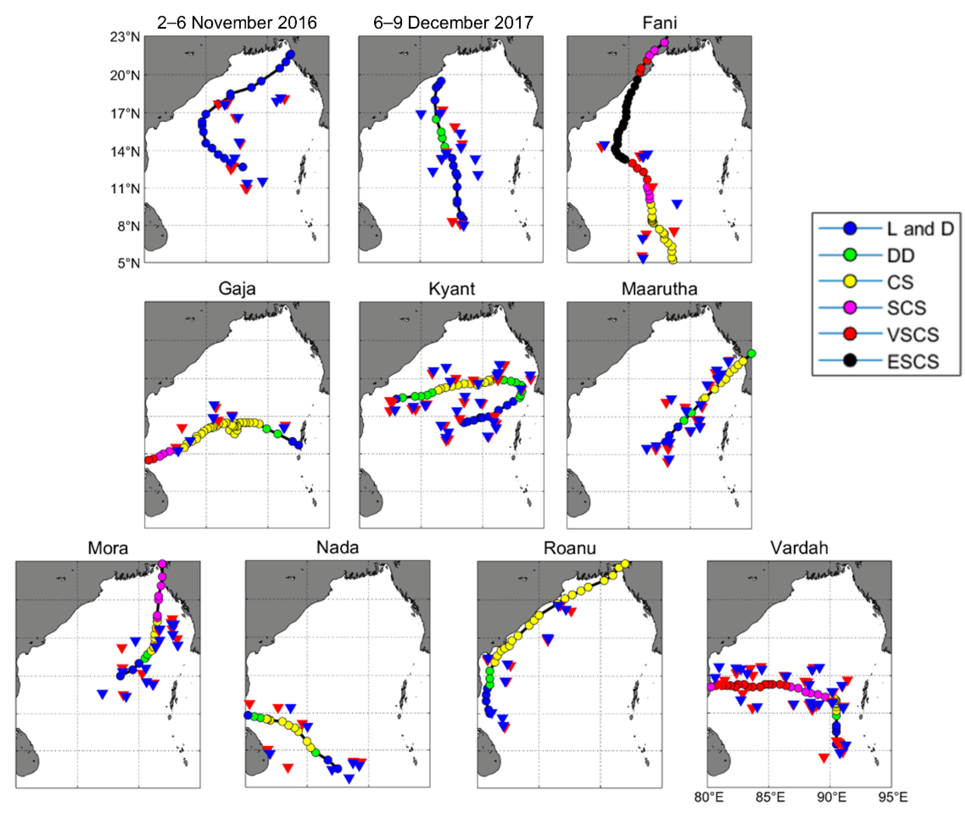
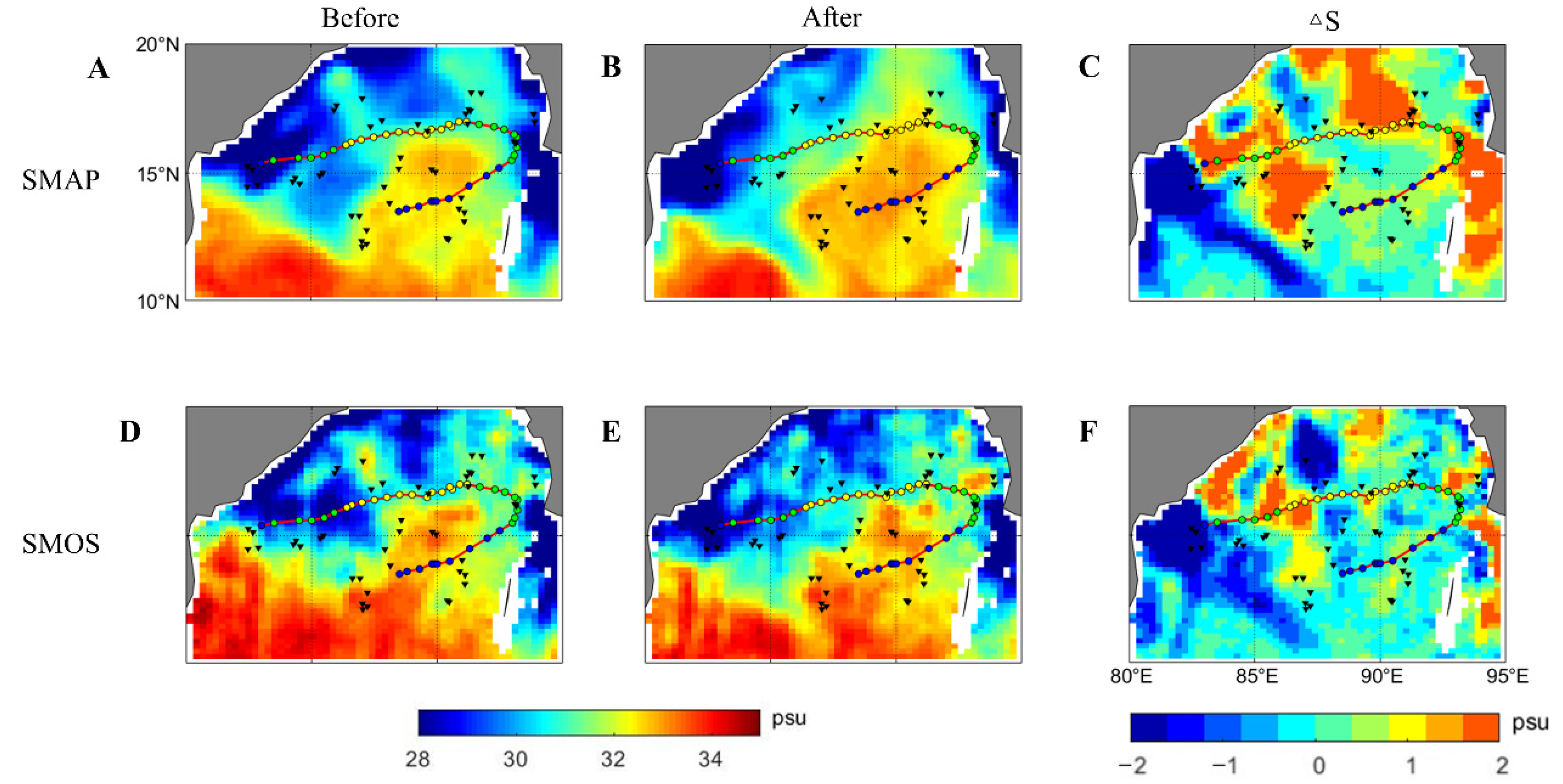
3.2. Impact of TC Roanu (2016) and TC Kyant (2016) on Retrieved Salinity from Satellite Products

TC Roanu (2016) in the coastal waters and TC Kyant (2016) in the open ocean of the BoB were selected as examples to analyze the influence of TCs on the retrieval of SMAP and SMOS salinity. TC Roanu developed over southwest BoB on 14 May 2016. Moving northeastward, it formed low pressure over southwest BoB and adjoining Sri Lanka on 15 May, then concentrated into a depression in southwest BoB on 17 May. TC Roanu moved northward and intensified to a deep depression on 18 May, then intensified as a cyclonic storm over western central BoB on 19 May. TC Roanu continued to move northeastward and skirt along the east coast of India. TC Kyant occurred as a depression over central southeastern BoB on 21 October 2016; the depression moved northeastward from 21 to 24 October. Then, it suddenly moved northwestward and intensified as a cyclonic storm over eastern central BoB on 25 October. TC Kyant kept moving southwest, then weakened and dissipated on 28 October 2016.
Figure 5 and Figure 6 show the retrieved salinity from SMAP and SMOS, and the salinity difference 8–9 days before and after TCs Roanu and Kyant. TC Roanu occurred in the pre-monsoon period (from 17 to 22 May 2016). Low-salinity (<32 psu) sea waters were only observed by SMAP and SMOS to the north of 20°N before and after TC Roanu. On the whole, SSMOS was higher than SSMAP, and the lower-salinity waters along the coast were mostly captured by SMAP. SSMAP worked better and agreed well with in situ SArgo on the coast of the BoB (R2 = 0.53) and reproduced a large part of the seasonal salinity variations [38]. Under the effect of TC Roanu, the salinity of coastal waters in the northwest BoB had small variations. The low salinity in the water in the northern bay was mainly due to rainfall and river discharge. Before and after TC Roanu passed, the salinity change of coastal waters was not very dramatic, and there was no large-scale increase in salinity. This was probably due to the compensation between the increased salinity caused by the TC (mixing and upwelling) and the decreased salinity caused by the large runoff and rainfall. There were 10 observations by Argo, which show that most SSMAP values were lower than in situ SArgo, but most SSMOS values were higher than SArgo (Figure 6). The average depth of in situ SArgo was 4.05 ± 2.15 m, which would lead to higher SArgo than the salinity of remote sensing observations.
TC Kyant occurred in the post-monsoon period (from 21 to 28 October 2016). There was a significant difference between the salinity in this period (Figure 7) and the pre-monsoon period (Figure 5): a larger area of lower-salinity waters (<28 psu) occupied the northern bay in the post-monsoon period. The passage of TC Kyant led to a large-scale increase in salinity along its track. This was mainly due to the strong TC-induced mixing and upwelling [17]. The correlations between SSMAP and SSMOS and SArgo were high (R2 = 0.82 for SMAP and 0.61 for SMOS). Figure 8 shows that SSMAP and SSMOS after TC Kyant passed mostly agree well with SArgo in the open ocean. Comparing SSMAP and SSMOS with the Argo in situ observations, the result shows that the former was overall better than the latter. These results are somewhat similar to those of a previous study in the tropical Pacific Ocean, showing that SMAP data had a higher correlation with TAO buoys than SMOS data [31]. After the SMOS data were updated from V3.0 to V5.0, the sea surface roughness correction model and retrieval algorithm were improved and the quality of SMOS data was greatly enhanced [19], but its retrieval is not as good as SMAP. This may be owing to the fact that the geophysical model function of SMAP in roughness correction is obtained from Aquarius [39], and the Aquarius can use radar data for roughness correction at high wind speeds. SMAP only provides salinity data from April 2015, while SMOS can provide valuable data for analyzing long-term series of salinity changes in the BoB from January 2010, effectively filling the SMAP gap.

4. Conclusions

Compared to the sea surface salinity data of Argo in the Bay of Bengal (BoB), this study assessed the accuracy of salinity products provided by level-3 Soil Moisture Active Passive (SMAP) V4.0 and debiased v5 CATDS level-3 Soil Moisture and Ocean Salinity (SMOS) for ~8 days before and after 10 tropical cyclones (TCs). The results show that both SMAP and SMOS could retrieve changes in sea surface salinity before and after the 10 TCs well. However, the retrieved salinity from SMAP was better than that from SMOS. Based on the evaluation of TC Roanu (2016) and TC Kyant (2016), the SMAP salinity data were basically consistent with the data from the in situ Argo observations in the coastal waters and open ocean in the BoB; in some cases, the retrieval of SMOS salinity data was inferior. In general, SMOS salinity data can fill the gap in SMAP satellite data from January 2010 to March 2015 and can provide more data for long-term salinity variability in the BoB.

Author Contributions

Conceptualization, H.X. and G.X.; formal analysis, Y.S.; investigation, H.X. and Y.S.; writing—original draft, Y.S.; writing—review and editing, H.X., G.X. and Y.S.; supervision, H.X. and G.X.; funding acquisition, H.X. All authors have read and agreed to the published version of the manuscript.

Funding

This research was funded by the Natural Science Foundation of China (42106148), Innovation Projects of Colleges and Universities in Guangdong Province (2021KQNCX028), scientific research start-up funds of Guangdong Ocean University (R20008), and the introduction and education program of “pilot plan” by the innovation and entrepreneurship term of Zhanjiang City (211207157080994).

Data Availability Statement

Satellite salinity data of level-3 Soil Moisture Active Passive V4.0 are available at http://www.remss.com/missions/smap/ (accessed on 1 October 2021). Satellite salinity data of debiased v5 CATDS level-3 Soil Moisture and Ocean Salinity can be accessed via https://www.catds.fr/Products/Available-products-from-CEC-OS/CEC-Locean-L3-Debiased-v5/ (accessed on 1 October 2021). The track data of tropical cyclones are available at http://www.rsmcnewdelhi.imd.gov.in/ (accessed on 1 October 2021). The Argo salinity data can be accessed via http://www.argodatamgt.org/ (accessed on 1 October 2021).

Acknowledgments

Argo data were obtained freely from the International Argo Program at http://www.argodatamgt.org/ (accessed on 1 October 2021). We are grateful to the academic editor and reviewers for constructive suggestions.

Conflicts of Interest

The authors declare that they have no competing or conflicts of interest to influence the work reported in this paper.

References

  1. Dube, S.K.; Rao, A.D.; Sinha, P.C.; Jain, I. Implications of climatic variations in the fresh water outflow on the wind-induced circulation of the Bay of Bengal. Atmos. Environ. 1995, 29, 2133–2138. [Google Scholar] [CrossRef]
  2. Vinayachandran, P.N.; Murty, V.S.N.; Babu, V.R. Observations of barrier layer formation in the Bay of Bengal during summer monsoon. J. Geophys. Res.-Oceans 2002, 107, C12. [Google Scholar] [CrossRef]
  3. Thadathil, P.; Muraleedharan, P.M.; Rao, R.R.; Somayajulu, Y.K.; Reddy, G.V.; Revichandran, C. Observed seasonal variability of barrier layer in the Bay of Bengal. J. Geophys. Res.-Oceans 2007, 112, C2. [Google Scholar] [CrossRef]
  4. Akhil, V.P.; Lengaigne, M.; Durand, F.; Vialard, J.; Chaitanya, A.V.S.; Keerthi, M.G.; Gopalakrishna, V.V.; Boutin, J.; Montegut, C.d.B. Assessment of seasonal and year-to-year surface salinity signals retrieved from SMOS and Aquarius missions in the Bay of Bengal. Int. J. Remote Sens. 2016, 37, 1089–1114. [Google Scholar] [CrossRef] [Green Version]
  5. Akhil, V.P.; Vialard, J.; Lengaigne, M.; Keerthi, M.G.; Boutin, J.; Vergely, J.L.; Papa, F. Bay of Bengal Sea surface salinity variability using a decade of improved SMOS re-processing. Remote Sens. Environ. 2020, 248, 111964. [Google Scholar] [CrossRef]
  6. Boutin, J.; Vergely, J.L.; Marchand, S.; D’Amico, F.; Hasson, A.; Kolodziejczyk, N.; Reul, N.; Reverdin, G.; Vialard, J. New SMOS Sea Surface Salinity with reduced systematic errors and improved variability. Remote Sens. Environ. 2018, 214, 115–134. [Google Scholar] [CrossRef] [Green Version]
  7. Sengupta, D.; Goddalehundi, B.R.; Anitha, D.S. Cyclone-induced mixing does not cool SST in the post-monsoon north Bay of Bengal. Atmos. Sci. Lett. 2008, 9, 1–6. [Google Scholar] [CrossRef]
  8. Neetu, S.; Lengaigne, M.; Vincent, E.M.; Vialard, J.; Madec, G.; Samson, G.; Kumar, M.R.R.; Durand, F. Influence of upper-ocean stratification on tropical cyclone-induced surface cooling in the Bay of Bengal. J. Geophys. Res.-Oceans. 2012, 117, C12. [Google Scholar] [CrossRef] [Green Version]
  9. Neetu, S.; Lengaigne, M.; Vialard, J.; Samson, G.; Masson, S.; Krishnamohan, K.S.; Suresh, I. Premonsoon/Postmonsoon Bay of Bengal Tropical Cyclones Intensity: Role of Air-Sea Coupling and Large-Scale Background State. Geophys. Res. Lett. 2019, 46, 2149–2157. [Google Scholar] [CrossRef]
  10. Grodsky, S.A.; Reul, N.; Lagerloef, G.; Reverdin, G.; Carton, J.A.; Chapron, B.; Quilfen, Y.; Kudryavtsev, V.N.; Kao, H.-Y. Haline hurricane wake in the Amazon/Orinoco plume: AQUARIUS/SACD and SMOS observations. Geophys. Res. Lett. 2012, 39, L20603. [Google Scholar] [CrossRef] [Green Version]
  11. Reul, N.; Quilfen, Y.; Chapron, B.; Fournier, S.; Kudryavtsev, V.; Sabia, R. Multisensor observations of the Amazon-Orinoco river plume interactions with hurricanes. J. Geophys. Res.-Oceans 2014, 119, 8271–8295. [Google Scholar] [CrossRef] [Green Version]
  12. Sun, J.; Vecchi, G.; Soden, B. Sea Surface Salinity Response to Tropical Cyclones Based on Satellite Observations. Remote Sen. 2021, 13, 420. [Google Scholar] [CrossRef]
  13. Reul, N.; Chapron, B.; Grodsky, S.A.; Guimbard, S.; Kudryavtsev, V.; Foltz, G.R.; Balaguru, K. Satellite Observations of the Sea Surface Salinity Response to Tropical Cyclones. Geophys. Res. Lett. 2021, 48, e2020GL091478. [Google Scholar] [CrossRef]
  14. Chacko, N. Insights into the haline variability induced by cyclone Vardah in the Bay of Bengal using SMAP salinity observations. Remote Sens. Lett. 2018, 9, 1205–1213. [Google Scholar] [CrossRef]
  15. Wang, X.; Yang, J.; Zhao, D.; Wang, X.; Sun, G. SMOS satellite salinity data accuracy assessment in the China coastal areas. Haiyang Xuebao 2013, 35, 169–176. (In Chinese) [Google Scholar]
  16. Yin, X.B.; Boutin, J.; Martin, N.; Spurgeon, P. Optimization of L-Band Sea Surface Emissivity Models Deduced From SMOS Data. IEEE Trans. Geosci. Remote Sens. 2012, 50, 1414–1426. [Google Scholar] [CrossRef]
  17. Xu, H.; Yu, R.; Tang, D.; Liu, Y.; Wang, S.; Fu, D. Effects of Tropical Cyclones on Sea Surface Salinity in the Bay of Bengal Based on SMAP and Argo Data. Water 2020, 12, 2975. [Google Scholar] [CrossRef]
  18. Meissner, T.; Wentz, F.J.; Manaster, A.; Lindsley, R. Remote Sensing Systems SMAP Ocean Surface Salinities [Level 2C, Level 3 Running 8-day, Level 3 Monthly], Version 4.0 validated release. Remote Sens. Syst. 2019. Available online: www.remss.com/missions/smap/ (accessed on 1 October 2021). [CrossRef]
  19. Boutin, J.; Vergely, J.L.; Khvorostyanov, D. SMOS SSS L3 maps generated by CATDS CEC LOCEAN. debias V5.0. SEANOE 2020. [Google Scholar] [CrossRef]
  20. Lin, X.; Qiu, Y.; Du, Y.; Zhou, X.; Xuan, L.; Xu, J. Study on the utilization of satellite remote sensing for variation characteristic of sea surface salinity in the Bay of Bengal. Haiyang Xuebao 2016, 38, 46–56. (In Chinese) [Google Scholar]
  21. Vidya, P.J.; Das, S.; Murali, M.R. Contrasting Chl-a responses to the tropical cyclones Thane and Phailin in the Bay of Bengal. J. Mar. Syst. 2017, 165, 103–114. [Google Scholar]
  22. Xu, H.; Tang, D.; Sheng, J.; Liu, Y.; Sui, Y. Study of dissolved oxygen responses to tropical cyclones in the Bay of Bengal based on Argo and satellite observations. Sci. Total Environ. 2019, 659, 912–922. [Google Scholar] [CrossRef] [PubMed]
  23. Remote Sensing Systems. New SMAP Sea Surface Salinity (SSS) 70 km Data. Available online: https://smap.jpl.nasa.gov/news/1265/smap-sees-sea-surface-salinity/ (accessed on 1 October 2021).
  24. Chacko, N. Chlorophyll bloom in response to tropical cyclone Hudhud in the Bay of Bengal: Bio-Argo subsurface observations. Deep. Sea Res. Part I Oceanogr. Res. Pap. 2017, 124, 66–72. [Google Scholar] [CrossRef]
  25. Xu, H.; Tang, D.; Liu, Y.; Li, Y. Dissolved oxygen responses to tropical cyclones “Wind Pump” on pre-existing cyclonic and anticyclonic eddies in the Bay of Bengal. Mar. Pollut. Bull. 2019, 146, 838–847. [Google Scholar] [CrossRef] [PubMed]
  26. Zhang, H.; Chen, D.; Zhou, L.; Liu, X.; Ding, T.; Zhou, B. Upper ocean response to typhoon Kalmaegi (2014). J. Geophys. Res. Ocean. 2016, 121, 6520–6535. [Google Scholar] [CrossRef]
  27. Price, J. Upper Ocean Response to a Hurricane. J. Phys. Oceanogr. 1981, 11, 153–175. [Google Scholar] [CrossRef] [Green Version]
  28. Potter, H.; Drennan, W.M.; Graber, H.C. Upper ocean cooling and air-sea fluxes under typhoons: A case study. J. Geophys. Res. Ocean. 2017, 122, 7237–7252. [Google Scholar] [CrossRef]
  29. Gonella, J. A rotary-component method for analysing meteorological and oceanographic vector time series. Deep. Sea Res. Oceanogr. Abstr. 1972, 19, 833–846. [Google Scholar] [CrossRef]
  30. Wright, C.W.; Walsh, E.L.; Vabdemark, D.; Krabill, W.B.; Garcia, A.W.; Houston, S.H.; Powell, M.D.; Black, P.G.; Marks, F.D. Hurricane Directional Wave Spectrum Spatial Variation in the Open Ocean. J. Phys. Oceanogr. 2001, 31, 2472–2490. [Google Scholar] [CrossRef]
  31. Bao, S.; Wang, H.; Zhang, R.; Yan, H.; Chen, J. Comparison of satellite-derived sea surface salinity products from SMOS, Aquarius and SMAP. J. Geophys. Res. Ocean. 2019, 124, 1932–1944. [Google Scholar] [CrossRef]
  32. Bao, S.; Wang, H.; Zhang, R.; Yan, H.; Chen, J. Spatial and temporal scales of sea surface salinity in the tropical Indian Ocean from SMOS, Aquarius and SMAP. J. Oceanogr. 2020, 76, 389–400. [Google Scholar] [CrossRef]
  33. Liu, S.S.; Sun, L.; Wu, Q.; Yang, Y.J. The responses of cyclonic and anticyclonic eddies to typhoon forcing: The vertical temperature-salinity structure changes associat ed with the horizontal convergence/divergence. J. Geophys. Res. Ocean. 2017, 122, 4974–4989. [Google Scholar] [CrossRef]
  34. Lin, X.; Qiu, Y.; Cha, J.; Guo, X. Assessment of Aquarius sea surface salinity with Argo in the Bay of Bengal. Int. J. Remote Sens. 2019, 40, 8547–8565. [Google Scholar] [CrossRef]
  35. Sabia, R.; Camps, A.; Vall-llossera, M.; Reul, N. Impact on Sea Surface Salinity Retrieval of Different Auxiliary Data Within the SMOS Mission. IEEE T. Geosci. Remote Sens. 2006, 44, 2769–2778. [Google Scholar] [CrossRef]
  36. Wang, J.; Jiao, Y.; Cao, Y.; Shi, J. Advances on ocean salinity remote sensing. Ocean Tech. 2006, 25, 76–81. (In Chinese) [Google Scholar]
  37. Bao, S.; Zhang, R.; Wang, H.; Yan, H.; Wang, Y. Correction of Satellite Sea Surface Salinity Products Using Ensemble Learning Method. IEEE Access 2021, 99, 1. [Google Scholar] [CrossRef]
  38. Alina, N.D.; Gaël, A.; Alex, C.S.; Adeola, B.; Arnaud, B. Global Analysis of Coastal Gradients of Sea Surface Salinity. Remote Sens. 2021, 13, 2507. [Google Scholar]
  39. Meissner, T.; Wentz, F.J.; Lee, T. Remote sensing systems SMAP ocean surface salinities [level 2C, level 3 running 8-day, Level 3 Monthly], Version 2.0 validated release. Remote Sens. Syst. 2019, 1–23. [Google Scholar] [CrossRef]
Figure 1. Tracks of 10 tropical cyclones (TCs) and positions of all selected Argo floats in Bay of Bengal (BoB) from April 2015 to December 2019. TC tracks are marked by solid red lines. (Note: blue, green, yellow, purple, red, and black dots represent low pressure (L) and depression (D), deep depression (DD), cyclonic storm (CS), severe cyclonic storm (SCS), very severe cyclonic storm (VSCS) and extremely severe cyclonic storm (ESCS), respectively, according to the India Meteorological Department. The red and blue inverted triangles represent the Argo floats before and after 10 TCs, respectively).
Remotesensing 14 03733 g001
Figure 2. Scatter map of Soil Moisture Active Passive Salinity (SSMAP), Soil Moisture and Ocean Salinity (SMOS), and Argo salinity (SArgo) data. (A,B) Correlation between SSMAP and SArgo before and after TCs, respectively; (C,D) correlation between SSOMS and SArgo before and after TCs, respectively. (Note: red dots represent the matched pairs before 10 TCs and blue dots represent the matched pairs after 10 TCs). Each dot represents collocated matched pairs and black lines show a 1:1 relationship. The linear correlation coefficients are significantly different from zero at 95% confidence (p-value).
Remotesensing 14 03733 g002
Figure 3. Scatter maps of SSMOS and SSMAP (A) before and (B) after passage of 10 TCs (indicated by red and blue dots, respectively).
Remotesensing 14 03733 g003
Figure 4. Scatter maps of SSMAP and SSMOS on left and right side of TC track after 10 TCs. Correlation after passage on (A) left side of TC track based on SMAP; (B) right side of TC track based on SMAP; (C) left side of TC track based on SMOS; (D) right side of TC track based on SMOS.
Remotesensing 14 03733 g004
Figure 5. Distribution of sea surface salinity of SMAP and SMOS (A,D) ~8 days before and (B,E) ~8 days after TC Roanu (2016), and (C,F) salinity difference of SMAP and SMOS between ~8 days before and after TC Roanu.
Remotesensing 14 03733 g005
Figure 6. Meridional salinity observations of Argo, SMAP, and SMOS after passage of TC Roanu (2016).
Remotesensing 14 03733 g006
Figure 7. Distribution of sea surface salinity of SMAP and SMOS (A,D) ~8 days before and (B,E) ~8 days after TC Kyant (2016), and (C,F) salinity difference of SMAP and SMOS between ~8 days before and after TC Kyant.
Remotesensing 14 03733 g007
Figure 8. Zonal salinity observations of Argo, SMAP, and SMOS after passage of TC Kyant.
Remotesensing 14 03733 g008
Table 1. Basic information about 10 TCs and correlations between SSMAP, SSMOS, and SArgo before and after TC passage in BoB.
DateMinimum Pressure (hPa)NameR2 of SSMAP and SArgo before TCsR2 of SSMAP and SArgo after TCsR2 of SSMOS and SArgo before TCsR2 of SSMOS and SArgo after TCs
17–22 May 2016983Cyclonic Storm Roanu0.53(8)0.85(10)0.38(8)0.67(10)
21–28 October 2016996Cyclonic Storm Kyant0.73(23)0.82(21)0.27(23)0.61(21)
2–6 November 20161000Depression0.88(9)0.93(9)0.74(9)0.78(9)
29 November–2 December 20161000Cyclonic Storm Nada0.97(7)0.86(7)0.98(7)0.93(7)
6–13 December 2016975VSCS Vardah0.90(26)0.53(22)0.78(26)0.27(22)
15–17 April 2017996Cyclonic Storm Maarutha0.85(13)0.80(15)0.43(13)0.30(15)
28–31 May 2017978SCS Mora0.51(11)0.43(14)0.68(11)0.04(14)
6–9 December 20171002Deep Depression0.87(7)0.85(10)0.54(7)0.94(10)
10–19 November 2018976VSCS Gaja0.60(6)0.15(6)0.46(6)0.35(6)
26 April–4 May 2019932ESCS Fani0.86(9)0.81(7)0.73(9)0.71(7)
Table 2. Comparison of satellite product (SSMAP and SSMOS) and Argo (SArgo) salinity data before and after 10 TCs. ∆ represents differences between Argo and satellite observations (SSMAP or SOMS-SArgo); bias represents mean difference (bias = Δ ¯ ). STD, standard deviation; RMSE, root mean square error.
SSMAP before TCsSArgo before TCsSSMOS before TCsSSMAP after TCsSArgo after TCsSSMOS after TCs
Mean ± STD (psu)32.33 ± 1.3932.44 ± 1.3432.60 ± 1.1632.64 ± 1.0032.65 ± 1.0332.59 ± 1.18
Bias (SMAP and Argo, psu)−0.11 −0.01
RMSE (SMAP and Argo, psu)0.58 0.47
Bias (SMOS and Argo, psu) 0.16 −0.06
RMSE (SMOS and Argo, psu) 0.84 0.78
Publisher’s Note: MDPI stays neutral with regard to jurisdictional claims in published maps and institutional affiliations.

