Abstract
In the modern electromagnetic environment, the intra-pulse modulations of radar emitter signals have become more complex. Except for the single-component radar signals, dual-component radar signals have been widely used in the current radar systems. In order to make the radar system have the ability to classify single-component and dual-component intra-pulse modulation at the same period of time accurately, in this paper, we propose a multi-label learning method based on a convolutional neural network and transformer. Firstly, the original single channel sampled sequences are padded with zeros to the same length. Then the padded sequences are converted to frequency-domain sequences that only contain the amplitude information. After that, data normalization is employed to decrease the influence of amplitude. After radar signals preprocessing, a designed model which combines a convolutional neural network and transformer is used to accomplish multi-label classification. The extensive experiments indicate that the proposed method consumes lower computation resources and has higher accuracy than other baseline methods in classifying eight types of single and thirty-six types of dual-component intra-pulse modulation, where the overall accuracy and weighted accuracy are beyond 90%.
1. Introduction
With the incensement in the number of radar systems, the modern electromagnetic environment has become more complex [1]. The intra-pulse modulation of radar emitter signals is an important part of electronic support measure systems, electronic intelligence systems and radar warning receivers [2,3,4]. Accurately classifying the intra-pulse modulation of radar emitter signals is beneficial for judging the threat level and analyzing the radar function [5]. As the radar systems become complicated, multi-component intra-pulse modulations have been employed for the radar signals, which increases the difficulty of classification.
The intra-pulse modulation classification methods based on deep learning [6] have been proposed in recent years. In [7], Kong et al. used Choi–William Distribution (CWD) images of low probability of intercept (LPI) radar signals and recognized the intra-pulse modulations. Similarly, Yu et al. [8] obtained the time-frequency images (TFIs) of the radar signal using CWD and extracted the contour of the signal in TFIs. After that, a convolutional neural network (CNN) model was trained with the contour images. In [9], Zhang et al. used Wigner–Ville Distribution (WVD) images of radar signals, which contain five types of intra-pulse modulations, to train the CNN model. In [10], Yu et al. firstly preprocessed the radar signal by Short-Time Fourier Transformation (STFT), and then, a CNN model was trained to classify intra-pulse modulation of radar signals. Wu et al. [11] designed a 1-D CNN with an attention mechanism to recognize seven types of radar emitter signals in the time domain, where the intra-pulse modulation of the signal is different. In [12], a 1-D Selective Kernel Convolutional Neural Network (SKCNN) was proposed to classify eleven types of intra-pulse modulations of radar emitter signals.
However, it could be seen from the above that the limitation is that the intra-pulse modulation classification mainly focuses on single-component intra-pulse modulation. As the intra-pulse modulation grows more complex than ever, multi-component intra-pulse modulation of radar emitter signals has been used in radar systems. Therefore, it is essential to take the cases in which multi-component intra-pulse modulation emerges in electromagnetic space into consideration. Some researchers have proposed methods, including blind source separation [13] and time-frequency analysis [14], but these methods require prior knowledge. With the development of deep learning, some methods based on convolutional neural networks have been proposed for classifying the multi-component intra-pulse modulations. Representative research is that Si et al. [15] used the smooth Pseudo-Wigner–Ville distribution (SPWVD) transformation to covert the dual-component radar signals into time-frequency images (TFIs), and then they used EfficientNet [16] to accomplish the multi-label classification tasks. The limitations of this method are that this method only focuses on the dual-component intra-pulse modulation, where the received signals may include single-component and dual-component intra-pulse modulation at the same time.
As the receivers of radar are passive, which means that both single-component and dual-component intra-pulse radar signals may be collected at the same period of time, it is not adequate for the classification system to only focus on single-component or dual-component intra-pulse modulation. Therefore, in order to reduce the mentioned limitation and make the radar system have the ability to classify single-component and dual-component intra-pulse modulation of radar emitter signals at the same period of time accurately, we proposed a multi-label learning method for accurately classifying single intra-pulse modulation and dual-component intra-pulse modulation of radar emitter signals.
In the experiments, the number of single-component intra-pulse modulations is set to be eight, including single-carrier frequency (SCF) signals, linear frequency modulation (LFM) signals, sinusoidal frequency modulation (SFM) signals, even quadratic frequency modulation (EQFM) signals, binary frequency shift keying (BFSK) signals, quadrature frequency shift keying (QFSK) signals, binary phase shift keying (BPSK) signals and Frank phase-coded (FRANK) signals. The dual-component intra-pulse modulations are generated by a random combination of each two single-component intra-pulse modulations, and the number of dual-component intra-pulse modulations is thirty-six, accordingly.
The framework of our method is shown as follows. Firstly, the original single channel sampled sequences are padded with zeros to the same length. Then, the padded sequences are converted to frequency-domain sequences that only contain the amplitude information. After that, data normalization is employed to decrease the influence of amplitude. After radar signals preprocessing, a designed model which combines a convolutional neural network and transformer is used to accomplish multi-label classification. The experiments show that in the situation of single-component and dual-component intra-pulse modulation existing at the same period of time, the proposed method consumes lower computation resources and has higher classification accuracy than other baseline methods.
The main contribution of this paper is that we focus not only on widely used single-component modulation but also on dual-component modulations, where the power for two-component modulations varies and the power ratio is not constantly 1:1. This work provides guidance and an effective approach for multi-label classification task on radar intra-pulse modulation. Another contribution is that we combined CNN and Transformer encoders, which makes better classification performance than the CNN-based structure only. The specific results can be seen in Section 5 and Section 6.
This paper is organized as follows: In Section 2, the related works about CNN in intra-pulse modulation classification and transformer in classification are introduced. Section 3 provides the information on the proposed method. The dataset and parameter settings are shown in Section 4. The extensive experiments and the corresponding analysis are described in Section 5. The ablation study and application scenarios of the proposed model are given in Section 6. Section 7 gives the conclusion.
2. Related Works
2.1. CNN in Radar Emitter Signal Intra-Pulse Modulation Classification
CNN has been widely used in image classification. The emergence of various CNN models made a great contribution to the improvement of classification accuracy. Many researchers have applied some of the CNN models to classify the intra-pulse modulation of radar emitter signals. Zhang et al. [9] used CNN to classify the intra-pulse modulations based on the Wigner-Ville Distribution (WVD) images of radar signals. Si et al. [15]. used a more effective model, EfficientNet, to classify the dual-component modulations based on the TFIs of SPWVD. Except for these 2-D CNN models, 1-D models were also applied. Wu et al. [11] proposed a 1-D CNN with an attention mechanism to classify five modulations of radar signals. Zhang et al. (Recognition of Noisy Radar Emitter Signals Using a One-Dimensional Deep Residual Shrinkage Network) proposed a 1-D DRSN, which could learn the features characterizing the signal directly. In our previous work [12], we designed a 1-D CNN model with selective kernel convolution layers and soft-attention parts, which has superior performance in the single-component modulation classification.
2.2. Transformer in Classification
Transformer [17] was originally proposed for natural language processing (NLP) tasks, which replaced the Recurrent Neural Network (RNN). In recent years, Transformer has been used in classification tasks. A guided transformer for classification is the vision transformer (ViT). ViT [18] divides an image into several patches as the input of the model, where the size of one patch is 14 × 14 or 16 × 16. The overview of ViT could be found in Figure 1. Swin Transformer [19] is one of the best transformer models, which uses window attention to combine both global and local information. The experiment results show that the transformer model could obtain a good classification accuracy when a huge number of samples is provided. However, when the number of samples is not so huge, the CNN models would perform better. In short, the transformer models lack inductive bias and need a huge number of samples to complete training [20].
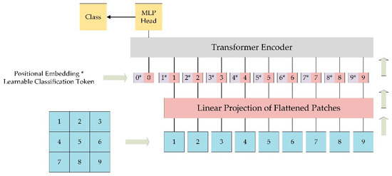
Figure 1.
The overview of ViT.
3. The Proposed Method
With the development of radar systems, except for single-component intra-pulse modulations, dual component intra-pulse modulations have been applied to new radar systems according to different functions. As the receivers of radar are passive, both single-component and dual-component intra-pulse modulation may be collected at the same period of time. In addition, the power ratio for two components of dual-component modulation varies according to different functions or purposes and is not constantly 1:1. Based on the above situation, in this paper, we proposed a multi-label learning method based on a convolutional neural network and transformer named CNN&Transformer to classify the single-component and dual-component intra-pulse modulation of radar emitter signals at the same time.
The method consists of the following parts: (1) Preprocess the raw single-channel sampled sequences. (2) Design the classification model based on a convolutional neural network and transformer. (3) Train the model with preprocessed samples.
3.1. The Architecture of Proposed CNN&Transformer
CNNs have been the dominant method of image since AlexNet [21] won the ImageNet competition. For intra-pulse modulation classification of radar emitter signals, there are two ways to design the CNN model. One is that convert the signals into 2-D TFIs and use two-dimensional (2-D) CNN models, where the classification task could be thought of as an image classification task. The second way is based on the feature of sampled radar signals, where the sequences are one-dimensional (1-D) and designed 1-D CNN-based model. To save the resource of computation and meet the real-time requirements to some degree, in this paper, we choose 1-D CNN as the backbones of the model.
Meanwhile, in recent years, Transformer [17] has been used in natural language processing tasks. Recently, researchers have employed the transformer in classification tasks. In [18], the author proposed a vision transformer (ViT) to classify the images. On the basis of ViT, some transformer models have been proposed for image classification tasks. Although these transformer models have been proved to have higher accuracy than CNN models, the limitations are that they are hard to train for computational cost and require much more data.
As the convolutional layer and pooling layer could extract features and reduce the size of the feature maps, and the transformer has been proved its effectiveness in classification tasks, inspired by [22], we combine the 1-D CNN with the transformer, which is hoped to combine the advantages of these two structures where CNN is faster, and transformer could bring better classification results, to classify both single-component and dual-component intra-pulse modulations. The overall architecture of the proposed model named CNN&Transformer is shown in Figure 2.
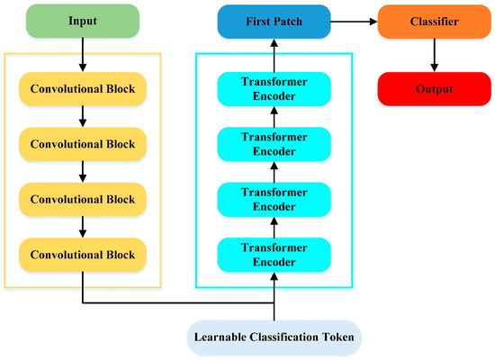
Figure 2.
The overall architecture of the proposed CNN&Transformer model.
The proposed model mainly contains two parts. The first part includes cascaded convolutional blocks, which extract feature from the input and provide the output feature maps in small size. The input feature maps in small size could reduce the computational cost of transformer. The second part is the cascaded transformer encoders, which are inspired by the original ViT that has a higher accuracy in image classification than traditional CNN.
Unlike the architecture of the original vision transformer shown in Figure 1, where the inputs are divided directly into several patches and the linear projection is on those patches, in our proposed CNN&Transformer, the CNN part extracts the features and outputs the input of the first transformer encoder. Compared with the operation of patch division, the CNN part, which is thought to have strong inductive bias [23], could make the input of the first transformer encoder more information. The classification results of the original transformer model could be found in Appendix A.3.
3.1.1. Convolutional Block
In this paper, there are four convolutional blocks in our proposed model, and the structure of the convolutional block is shown in Figure 3.
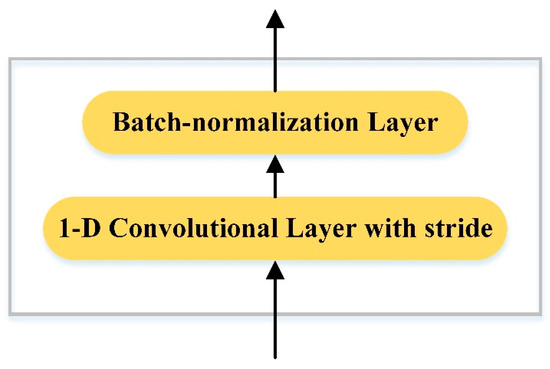
Figure 3.
The structure of convolutional block.
Each convolutional block includes a 1-D convolutional layer with stride and a batch-normalization layer [24]. Given an input sequence where refers to the length of sequence and refers to the channel number of sequence (For the first convolutional block, the value of is 1), the 1-D convolutional layer with a stride in the convolutional block will extract features and output the feature maps with less length. The output feature maps of the convolutional block could be obtained after batch-normalization layer. This process could be written as:
where and refer to the operation of 1-D convolution with stride and batch normalization, respectively. and are the corresponding result of these operations. Typically, the value of is smaller than that of , and the value of is larger than that of .
3.1.2. Transformer Encoder
There are four cascaded transformer encoders in the transformer part. Before feeding into the transformer part, a learnable classification token [25] is concatenated together with . This process could be written as:
where , to are the patches of with length and the length of each patch is .
In [18], position information was added by 1-D or 2-D positional encodings. As the front of the model is convolution, which contains the positional information [26], in this paper, there is no extra positional encodings.
The result is passed to the transformer encoders. The structure of transformer encoder is shown in Figure 4.
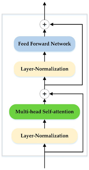
Figure 4.
The structure of transformer encoder.
Each transformer encoder includes a layer-normalization layer [27], a multi-head self-attention block, a layer-normalization layer and a feed forward network. Firstly, layer-normalization is employed to normalize , and the result could be written as:
where refers to the operation of layer normalization.
The multi-head self-attention block could be thought of as the concatenation of several single-head self-attention module. In the single-head self-attention module, for the given input , there are three trainable matrices named , and . The query, key and value for each patch of could be obtained by:
where is the i-th patch of . Then we calculate the inner product to match and , and normalize the result with the scale . The result could be shown as:
After that, SoftMax operation is employed to , and this process could be written as:
The result of could be thought of as the weights for , and the output could be written as:
Accordingly, in the form of matrix, the query matrix, key matrix and value matrix could be written as:
The output of a single self-attention module could be written as:
The multi-head self-attention block computes separately for times, where the value of is . Therefore, the output of the transformer encoder consists of number of independent . This could be written as:
Before feeding to the layer-normalization layer, there is a residual part that the original and could be fused together. This process could be written as:
Then, the result is sent to a two-layer fully connected neural network with “ReLU” activation function in the feed forward network. The second residual part fuses and the output of feed forward network. This process could be written as:
where refers to the output of the first transformer encoder, refers to the two-layer fully connected neural network.
The transformer encoders are cascaded, and we slice the first patch of the output in the last transformer encoder for the classification, which corresponds to the learnable classification token . This could be written as:
where refers to the output of the last transformer encoder.
3.2. Data Preprocessing
In this paper, we assume that the collected radar emitter signals vary in a certain range. The sampling way is single channel sampling, which could reduce the requirement and complexity of the sampling hardware compared with IQ sampling. The signal could be written as:
where refers to the pure radar signal and the intra-pulse modulation includes one or two components. is the additional white Gaussian noise (AWGN) [28]. Single-component and dual-component intra-pulse modulation are widespread on the real battlefield, and the power ratio for two-component of dual-component modulation varies according to different functions or purposes and is not constantly 1:1, which means that each component of dual-component modulation is not the same signal-to-noise ratio (SNR) under the same noise sequence.
Once the sampling frequency is given, the length of sampled signals will be determined. We firstly pad zero to the end of the original single channel sampled sequences and ensure that the padded sequences are of the same length. Then the padded sequences are converted to frequency-domain sequences that only contain the amplitude information. This process could be written as:
where refers to the original single channel sampled sequences, refers to discrete Fourier transformation and refers to the process of calculating the absolute value.
After that, data normalization is employed to decrease the influence of amplitude. This could be written as:
where ranges from 0 to 1. refers to the process of finding the max value of a given input sequence.
4. Dataset and Experiment Setting
In this section, a simulation dataset is introduced. In addition, the parameters of the proposed CNN&Transformer are shown in detail. A computer with Intel 10900K, 128GB RAM, RTX 3070 GPU hardware capabilities, “MATLAB 2021a” software, “Keras” and “Python” programming language have been used. “MATLAB 2021a” was used to generate the simulated dataset. “Keras” and “Python” were used for developing the model.
4.1. Dataset
In our experiments, the simulation dataset will be used to train and test the proposed method and other baseline methods. The sampling way is single channel sampling, and the sampling frequency is 1 GHz. Although in the real battlefield, the pulse width could range from several microseconds to hundred microseconds, in this paper, we only focus on a certain range of pulse width, which ranges from 5 us to 30 us.
Eight single-component intra-pulse modulations are generated, and their parameters are shown in Table 1.

Table 1.
Parameters of eight single-component intra-pulse modulations.
The carrier frequency and bandwidth in the table is the normalized frequency based on the single channel sampling frequency. For instance, if the carrier frequency is 0.2 or the bandwidth is 0.3, the according to carrier frequency and bandwidth based on the sampling frequency will be 200 MHz or 300 MHz, respectively. In addition, the sampled signals are discrete real signals with a length of 5000–30,000 points.
For the dual-component intra-pulse modulation of radar emitter signals, their modulations are based on the combinations of single-component intra-pulse modulation. Therefore, the number of single-component intra-pulse modulation is eight, and the number of dual-component intra-pulse modulation is thirty-six. In addition, the power for two-component modulations varies, and the power ratio of low-power component modulation and high-power component modulation ranges from 1:3 to 1:1, which provides better wider coverage than only a 1:1 power ratio.
To make the analysis of experiments in the next sections easier, we provide the index information for the modulation in Table 2 and Table 3.
Table 2.
The index information for the single-component modulation.
Table 3.
The index information for the dual-component modulation.
The SNR is defined as , where and are the pure signal power and AWGN power, respectively. The SNR ranges from −14 dB to 0 dB, with 2 dB increment. Every 2 dB, 400 samples, 100 samples and 200 samples for each type of intra-pulse modulation are generated for training, validation, and testing, respectively. Therefore, the training dataset, validation dataset and testing dataset include 140,800 samples, 35,200 samples and 70,400 samples, respectively.
Figure 5 shows the preprocessed results of six modulation samples in SID3, SID4, ID6, ID12, ID17 and ID19 when SNR is 0 dB. In order to make the samples more visible, the TFIs of these samples based on SPWVD in [15] are shown in Figure 6.
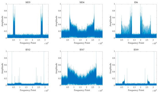
Figure 5.
The preprocessed result of six modulation samples in SID3, SID4, ID6, ID12, ID17 and ID19 when SNR is 0 dB.
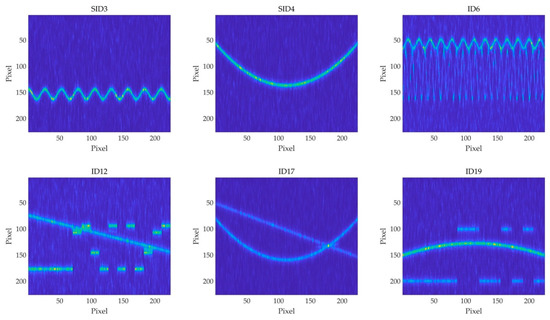
Figure 6.
The TFIs of six modulation samples in SID3, SID4, ID6, ID12, ID17 and ID19 based on SPWVD when SNR is 0 dB.
4.2. Experiment Setting
4.2.1. Multi-Hot Labelling
In this paper, we choose to label the sample in a multi-hot way. As there are single-component intra-pulse modulations, the labeling way should be adjusted compared with the way in [15]. Each label contains nine elements, and the first eight elements refer to the modulation the signals belong to. The last element is the mark whether the signal is in single-component modulation or dual-component modulation, where “0” refers to single-component modulation and “1” refers to dual-component modulation. For instance, a sample with a label vector means this sample is in dual-component modulation and the two components are all the first single intra-pulse modulation. The sample with a label vector means this sample is in single-component modulation and the component is the second single intra-pulse modulation.
4.2.2. Parameters of the Proposed CNN&Transformer
Based on the sampling frequency and pulse width, the length of sample sequences ranges from 5000 to 30,000 points. We set the length for padded sequences as 32,768, which could accelerate the processing of DFT [29]. Therefore, the input shape of the proposed model is 32,768.
The kernel size in each convolutional layer is 16. The number of filters in four convolutional blocks is 16, 32, 64 and 128. The convolutional stride in all the convolutional layers is set to be 4. Activation function is “ReLU” [30]. The number of heads in multi-head self-attention module is set to be 8. The first layer in the feed forward neural network contains 384 nodes, and the second layer contains 128 nodes, with “ReLU” activation function. The sliced patches of the output in the last transformer encoder will be fully connected with the output layer with nine nodes, where the activation function is “Sigmoid”.
4.2.3. Baseline Methods
The method used in [15], named CNN-SPWVD, is based on SPWVD of time-frequency analysis and will be selected and carried out as a baseline method using the simulated dataset. As other deep learning-based methods mainly focus on single-component intra-pulse modulation classification, we adjust some of these methods to make the model suitable for the multi-label learning classification task, specifically, 1-D SKCNN in [12], where the size of selective kernels are 16 and 9, respectively, the pooling size and pooling stride are adjusted as 7 and 7. The nodes of the first hidden layer of MLP in each selective convolutional block in 1-D SKCNN are 8, 16, 32, and 64, respectively. Moreover, the nodes of the full connection unit are 256.
In addition, although the method in [10], which used the TFIs of STFT based on time-frequency analysis, only aims to classify single-component intra-pulse modulations, this method is still applied as a baseline method, where the model is replaced by EfficientNet and changing the number of nodes in the output layer, which is named CNN-STFT. The method in [7] used TFIs of CWD; however, the model is quite simple. Therefore, EfficientNet is used to replace the original model, and this method is named CNN-CWD. The above time-frequency analysis tools are widely used in radar signal analysis and have been proved effective in intra-pulse modulation classification based on the mentioned literature.
In order to evaluate the effectiveness of the transformer encoder, we replace the transformer part with one convolutional block with 256 filters, where the stride in convolutional layer is 4, and add a full connect layer with 256 nodes, named CNN-Normal. Table 4 summarizes the name of methods with the according used input data and models in the experiments.
Table 4.
The name of the methods in experiments with the according used input data and models.
5. Experimental Results
5.1. Training Details
During the training sections, the loss function is binary cross-entropy. The optimization algorithm is set as adaptive moment estimation (ADAM) [31]. The batch size is set as 32, epochs as 50 with 0.001 learning rate. After training 50 epochs, another 10 training epochs with a 0.0001 learning rate are carried out. The influence of batch size on the efficiency of model training could be found in Appendix A.2. The weights for testing sections are chosen, which have the highest overall classification accuracy for the intra-pulse modulations on the validation dataset. As the output layer uses the “Sigmoid” activation function, the threshold for binarization is set as 0.5, and this process could be written as:
where is the result after binarization and is the output the model and the length is 9, which is equal to the length of the multi-hot label.
For traditional multi-label classification tasks, the metrics are insensitive to label imbalance, where recall, precision, F1-score and other metrics are included. However, for the radar system, the major demand is the classification accuracy, which means that both the number of components and the component itself, the classification system provided should exactly match the actual situation. Less classification and misclassification would make errors and increase the probability of being threatened by radar systems. Therefore, accuracy is used as the main metric for saving the best weights. As the numbers of single-component and dual-component intra-pulse modulation signals are not the same, where the ratio of the number is 8:36, it is important to balance the weight for evaluating classification performance. Therefore, in this paper, except for the overall classification accuracy, the weighted classification accuracy is also included, and the calculation for the weighted classification accuracy could be written as:
where and refers to the classification accuracy for single-component and dual-component intra-pulse modulations, respectively.
For the testing section, other metrics, including Hamming loss, recall, precision and F1-score, will be used to evaluate the methods comprehensively.
5.2. Experimental Results of the Proposed Method and Baseline Methods
Our proposed model and the baseline models were trained based on the datasets in Section 4.1. Firstly, the classification performance of eight single-component and thirty-six dual-component intra-pulse modulation of radar emitter signals based on the mentioned methods is shown in Figure 7. In addition, Table 5 gives the statistical results including average accuracy, Hamming loss, recall, precision and F1-score at macro level and micro level. Additionally, Figure 8 shows both the overall classification accuracy and weighted classification accuracy of these methods based on different SNRs.
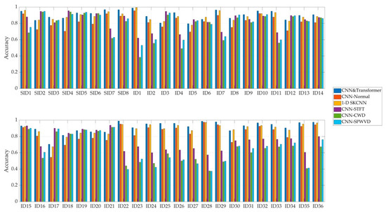
Figure 7.
The average classification accuracy of eight single-component and thirty-six dual-component intra-pulse modulation of radar emitter signals based on the mentioned methods.
Table 5.
The statistical results including average accuracy, Hamming loss, recall, precision and F1-score in macro level and micro level of the mentioned methods.
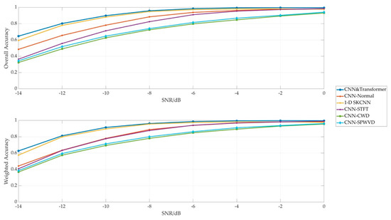
Figure 8.
The overall classification accuracy and weighted classification accuracy of the methods based on different SNR.
As the results show, the proposed CNN&Transformer performs best among the mentioned methods. For the 1-D methods, CNN-Normal performs worst, which shows that the simple CNN structure could not meet the demand of classification of intra-pulse modulation.
For these TFI-based CNN methods, CNN-STFT has the highest classification accuracy on both single-component and dual-component modulations, where both overall classification accuracy and weighted classification accuracy are at least 5% higher than the second best TFI-based CNN method named CNN-SPWVD. In addition, it could be found that all these three TFI-based methods have better classification accuracy on single-component modulations than that on dual-component modulations. However, the performance of 1-D SKCNN and CNN&Transformer is superior to these three TFI-based methods.
Generally, the classification accuracy increases when SNR improves. Compared with other methods, it could be found that the TFI-based methods are more vulnerable when the noise is strong. Additionally, even in the extreme situation where the SNR is −14 dB, the accuracy of the proposed CNN&Transformer is about 5% higher than the second best model 1-D SKCNN, which shows the superiority of our proposed method.
Although TFI-based methods have better classification performance on some types of intra-pulse modulation than CNN&Transformer, for instance, SID2, ID5 and ID15. However, their average classification accuracy for other modulations is much lower, where the biggest classification accuracy gap could be up to 60%. We also evaluate the accuracy stabilization of the methods with a series of accuracy thresholds. The average classification accuracy for 44 types of modulation that is less than 80%, 82.5% and 85% based on the mentioned models is calculated, and the results are shown in Table 6.
Table 6.
The average classification accuracy for 44 types of modulation that is less than 80%, 82.5% and 85%, based on the mentioned models.
According to Table 6, we could find that even for the higher accuracy threshold, our proposed CNN&Transformer is still more robust and more stable, with minimum number of times where the average classification accuracy is below the threshold.
Therefore, in terms of classification accuracy, our proposed CNN&Transformer is more competitive and superior to the mentioned methods.
5.3. Time Usage and Storage Space
In this section, we will evaluate the time usage and storage space of our proposed method and the baseline methods. For time usage, there are two main parts: the time of data preprocessing and the train time. For the storage space usage, the parameters (Params) of the model are focused on.
Specifically, the time usage at the data preprocessing stage is shown in Table 7. In addition, Table 8 gives the Params, floating point operations (FLOPs) and the training time per epoch of the mentioned methods.
Table 7.
The data preprocessing time between TFI-based methods and 1-D-model-based method.
Table 8.
The parameters, floating point operations and the training time per epoch of the mentioned models.
Table 7 shows that the data preprocessing time of CNN-STFT, CNN-CWD and CNN-SPWVD is around 3 times, 54 times and 57 times, respectively, than that of 1-D model-based methods. In addition, the length of the original sampled sequence ranges from 5000 to 30,000 points. The input shape of 1-D based model is a 32,768-length vector. However, the input shape of the TFI-based model is a matrix with 224 × 224 dimension that requires 1.5 times more space to save TFIs data compared with 1-D-based methods. Based on the mentioned analysis, it could be found that the 1-D model-based method has advantage of higher speed and low storage usage in data preprocessing stage.
According to Table 8, it is shown that compared with the baseline methods, our proposed CNN&Transformer is faster in training sessions. Additionally, when making a comparison among the CNN-Normal and our proposed CNN&Transformer model, we could easily find that the combination of CNN and transformer structure has the advantage of higher classification accuracy and limited computation resource.
6. Discussion
We further analyzed the influence of the number of transformer encoders and the number of heads in the multi-head self-attention module on the classification accuracy. The ablation experiments are based on the same dataset in Section 4.1, where the training setting is the same as in Section 5.1. In addition, we provide some scenarios of how our method could be applied. The effectiveness and rationality analysis of proposed CNN&Transformer could be found in Appendix A.1.
6.1. Ablation Study on the Number of Transformer Encoder and Head in Multi-Head Self-Attention Module
We change the number of transformer encoders. The encoder number is 1, 2, 4, 8 and 12. The head number for these five models is 1, 2, 4, 8 and 16, respectively. The classification accuracy, the Params, FLOPs and training time are shown in Table 9.
Table 9.
The classification accuracy, parameters, floating point operations and training time for the CNN-Transformer with different numbers of encoders and different numbers of heads.
The experimental result shows that more transformer encoders will bring better classification accuracy. It could be found that with an increment of the number of transformer encoders, the classification accuracy of intra-pulse modulation improves, especially when the number of encoders changes from 1 to 2. The accuracy improvement grows slowly when the number of encoders is already large. Additionally, the training time increases around 16 s when an extra transformer encoder is added.
Moreover, it could be found that when the encoder number is small, more heads in the multi-head self-attention module could increase the classification accuracy. For instance, the accuracy increases by nearly 3% when the head number increases from 1 to 16 in the one-encoder CNN&Transformer model. However, when the encoder number is large, the influence of head number on accuracy is little, and more heads may lead to a slight fallback in classification accuracy
In terms of the training time and classification accuracy, the structure with four transformer encoders and eight heads in the multi-head self-attention module, which does not bring too much extra time, is more suitable for this paper.
6.2. Application Scenarios
CNN and transformer have been widely used in image classification and other downstream tasks. CNN is thought to be good at extracting local information while the transformer is thought to be good at extracting global information. The existed literature has proved that it is much harder to train a whole transformer compared with CNN but the performance of a well-trained transformer is better than CNN. We combine both CNN and transformer to classify both single-component and dual-component intra-pulse modulation of radar emitter signals at the same time. Through the results of Table 5, Table 6, Table 7, Table 8 and Table 9, we could get a conclusion, the combination of CNN and transformer could increase the classification performance on single-component and dual-component intra-pulse modulation of radar emitter signals. Additionally, in real applications, radar systems have higher real-time requirements. Therefore, there is no need to make the model larger to improve its performance. A better solution to increase the classification performance is using the limited parameters and computation resources, and our proposed method has better performance in this regard.
At the same time, our method could be applied to other modulation classification tasks in semi-supervised situations. Currently, there are few pieces of literature focusing on semi-supervised classification of intra-pulse modulations of radar signals. We could use our proposed model to complete these kinds of tasks.
7. Conclusions
In this paper, we proposed a multi-label learning method based on the combination of CNN and Transformer for classifying both eights single-component and thirty-six dual-component intra-pulse modulations of radar emitter signals at the same time. The comparisons with other baseline methods in classification performance with accuracy, Hamming loss, recall, precision and F1-score in macro level and micro level, storage usage and computation resource show that our proposed method is superior and the combination of CNN and transformer is more effective than the CNN-based structure only. Additionally, according to the ablation study on the number of transformer encoders and the number of heads in multi-head self-attention module, we could conclude that when time permits, more encoders and more heads in a certain range could increase the classification performance. Our method provides guidance for multi-label classification tasks on intra-pulse modulation in radar systems.
In further work, we will attempt to optimize the structure of the proposed model and apply it to classify more complex multi-component intra-pulse modulations of radar emitter signals. Moreover, applying this framework to real radar systems and increasing the classification accuracy further is another problem in the future.
Author Contributions
Conceptualization, S.Y. and B.W.; methodology, S.Y. and B.W.; software, S.Y.; validation, S.Y.; formal analysis, P.L. and S.Y.; investigation, S.Y. and B.W.; resources, P.L.; data curation, S.Y.; writing—original draft preparation, S.Y.; writing—review and editing, S.Y.; supervision, P.L. All authors have read and agreed to the published version of the manuscript.
Funding
This research received no external funding.
Data Availability Statement
Data sharing is not applicable.
Conflicts of Interest
The authors declare no conflict of interest.
Appendix A
In Appendix A section, in order to show the stabilization of the proposed model, we train the proposed model nine more times to capture the mean accuracy with uncertainty, and the results can be seen in Appendix A.1. Appendix A.2 provides the analysis of the influence of batch size on the efficiency of model training.
Appendix A.1. Effectiveness and Rationality Analysis of Proposed CNN&Transformer
In this section, we train the proposed CNN&Transformer model (four encoders with eight heads) nine more times to capture the mean accuracy with uncertainty. The dataset and training details are the same as in Section 5.1. Table A1 shows the accuracy of the original experiment and five additional experiments.
Table A1.
The classification accuracy of the original experiment and five additional experiments.
Table A1.
The classification accuracy of the original experiment and five additional experiments.
| Experiment | Single Component | Dual Component | Overall Accuracy | Weighted Accuracy |
|---|---|---|---|---|
| Original | 0.9146 | 0.9087 | 0.9098 | 0.9116 |
| 1st Time | 0.9016 | 0.9104 | 0.9088 | 0.9060 |
| 2nd Time | 0.9120 | 0.9091 | 0.9096 | 0.9105 |
| 3rd Time | 0.9099 | 0.9091 | 0.9093 | 0.9095 |
| 4th Time | 0.9066 | 0.9093 | 0.9088 | 0.9080 |
| 5th Time | 0.9188 | 0.9072 | 0.9093 | 0.9130 |
| 6th Time | 0.9055 | 0.9094 | 0.9087 | 0.9074 |
| 7th Time | 0.9078 | 0.9080 | 0.9080 | 0.9079 |
| 8th Time | 0.9070 | 0.9098 | 0.9093 | 0.9084 |
| 9th Time | 0.9062 | 0.9091 | 0.9086 | 0.9076 |
| Average | 0.9090 | 0.9090 | 0.9090 | 0.9090 |
| Standard Deviation | 0.0045 | 0.0008 | 0.0005 | 0.0019 |
According to Table A1, it could be found that the mean average accuracy from a different view is beyond 90%, and the value of standard deviation is low. The additional experimental results show that the proposed CNN&Transformer model could converge on average to a corresponding result, which provides evidence of the effectiveness and rationality of our proposed model.
Appendix A.2. The Influence of Batch Size on the Efficiency of Model Training
In this section, we train the proposed CNN&Transformer model (four encoders with eight heads) with different batch sizes. The training details are the same as in Section 5.1 except for batch size.
The training epoch is set to be 50, where the learning rate is 0.001 with the ADAM optimizer. Unlike Section 5.1, in these experiments, the addition 10 epochs are not added. Table A2 shows the training time per epoch. The accuracy of the validation dataset at the end of each training epoch according to different batch sizes is shown in Figure A1.
Table A2.
The training time per epoch based on different batch sizes.
Table A2.
The training time per epoch based on different batch sizes.
| Batch Size | 16 | 32 | 64 | 128 | 256 |
|---|---|---|---|---|---|
| Time per epoch | 238 s | 129 s | 94 s | 81 s | 77 s |
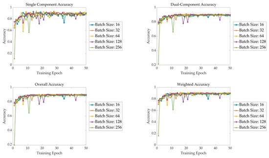
Figure A1.
The accuracy of validation dataset at the end of each training epoch according to different batch size.
According to Table A2, it could be found that a large number of batch size, which leads to fewer training iterations per epoch, could reduce the time usage per training epoch. However, due to the GPU hardware limitation, the trend of training acceleration is not linear with batch size. Additionally, Figure A1 indicates that small or large value of batch size in some cases is not stable, where the validation accuracy based on these values of batch size may fall several times. However, if the hardware is permitted, it is recommended to increase the value of batch size, which could make the most of computation resources, and set a large value of training epoch to enlarge the training iterations.
Appendix A.3. The Classification Results Based on The Original Transformer Model
In this section, we conduct the experiment based on the original transformer model. Like the patch division in Figure 1, we design three models, where the number of the transformer encoder is set to be 4 with 8 heads, 8 with 8 heads and 12 with 8 heads, respectively. The number of patches is set to 128, where the length of each patch is 256. After the linear projection, each patch will be converted to a vector with a length of 128, which is the same to the length of input before the first transformer encoder in our proposed CNN&Transformer model. The training details are the same as in Section 5.1. Table A3 gives the classification accuracy of testing dataset, including single-component accuracy, dual-component accuracy, overall accuracy and weighted accuracy.
Table A3.
The classification accuracy of testing dataset.
Table A3.
The classification accuracy of testing dataset.
| Encoder Number | Single Component | Dual Component | Overall Accuracy | Weighted Accuracy |
|---|---|---|---|---|
| 4 | 0.8268 | 0.8356 | 0.8340 | 0.8312 |
| 8 | 0.8263 | 0.8344 | 0.8329 | 0.8303 |
| 12 | 0.8321 | 0.8423 | 0.8405 | 0.8372 |
Table A3 indicates that the original architecture of transformer model could not perform well in classifying the intra-pulse modulations, where its accuracy is quite close to that of the CNN-Normal in Section 5.2. Compared with our proposed CNN&Transformer model, we could conclude that the combination of CNN and transformer could improve the performance of model in classifying intra-pulse modulations of radar emitter signals.
References
- Gupta, M.; Hareesh, G.; Mahla, A.K. Electronic Warfare: Issues and Challenges for Emitter Classification. Def. Sci. J. 2011, 61, 228. [Google Scholar] [CrossRef] [Green Version]
- Barton, D.K. Radar System Analysis and Modeling; Artech: London, UK, 2004. [Google Scholar]
- Richards, M.A. Fundamentals of Radar Signal Processing, 2nd ed.; McGraw-Hill Education: New York, NY, USA, 2005. [Google Scholar]
- Wiley, R.G.; Ebrary, I. ELINT: The Interception and Analysis of Radar Signals; Artech: London, UK, 2006. [Google Scholar]
- Wang, X. Electronic radar signal recognition based on wavelet transform and convolution neural network. Alex. Eng. J. 2022, 61, 3559–3569. [Google Scholar] [CrossRef]
- Schmidhuber, J. Deep Learning in Neural Networks: An Overview. Neural Netw. 2015, 61, 85–117. [Google Scholar] [CrossRef] [PubMed] [Green Version]
- Kong, S.-H.; Kim, M.; Hoang, L.M.; Kim, E. Automatic LPI Radar Waveform Recognition Using CNN. IEEE Access 2018, 6, 4207–4219. [Google Scholar] [CrossRef]
- Yu, Z.; Tang, J. Radar Signal Intra-Pulse Modulation Recognition Based on Contour Extraction. In Proceedings of the IGARSS 2020–2020 IEEE International Geo-science and Remote Sensing Symposium, Waikoloa, HI, USA, 26 September–2 October 2020; pp. 2783–2786. [Google Scholar] [CrossRef]
- Zhang, J.; Li, Y.; Yin, J. Modulation classification method for frequency modulation signals based on the time–frequency distribution and CNN. IET Radar Sonar Navig. 2018, 12, 244–249. [Google Scholar] [CrossRef]
- Yu, Z.; Tang, J.; Wang, Z. GCPS: A CNN Performance Evaluation Criterion for Radar Signal Intrapulse Modulation Recognition. IEEE Commun. Lett. 2021, 25, 2290–2294. [Google Scholar] [CrossRef]
- Wu, B.; Yuan, S.; Li, P.; Jing, Z.; Huang, S.; Zhao, Y. Radar Emitter Signal Recognition Based on One-Dimensional Convolutional Neural Network with Attention Mechanism. Sensors 2020, 20, 6350. [Google Scholar] [CrossRef]
- Yuan, S.; Wu, B.; Li, P. Intra-Pulse Modulation Classification of Radar Emitter Signals Based on a 1-D Selective Kernel Convolutional Neural Network. Remote Sens. 2021, 13, 2799. [Google Scholar] [CrossRef]
- Zhu, H.; Zhang, S.; Zhao, H. Single-channel source separation of multi-component radar signal based on EVD and ICA. Digit. Signal Process. 2016, 57, 93–105. [Google Scholar] [CrossRef]
- Zhu, D.; Gao, Q.; Lu, Y.; Sun, D. A signal decomposition algorithm based on complex AM-FM model. Digit. Signal Process. 2020, 107, 102860. [Google Scholar] [CrossRef]
- Si, W.; Wan, C.; Deng, Z. Intra-Pulse Modulation Recognition of Dual-Component Radar Signals Based on Deep Convolutional Neural Network. IEEE Commun. Lett. 2021, 25, 3305–3309. [Google Scholar] [CrossRef]
- Tan, M.; Le, Q. EfficientNet: Rethinking model scaling for convolutional neural networks. Proc. Int. Conf. Mach. Learn. 2019, 97, 6105–6114. [Google Scholar]
- Vaswani, A.; Shazeer, N.; Parmar, N.; Uszkoreit, J.; Jones, L.; Gomez, A.N.; Kaiser, Ł.; Polosukhin, I. Attention is all you need. In Proceedings of the Advances in Neural Information Processing Systems, Long Beach, CA, USA, 4–9 December 2021; pp. 5998–6008. [Google Scholar]
- Dosovitskiy, A.; Beyer, L.; Kolesnikov, A.; Weissenborn, D.; Zhai, X.; Unterthiner, T.; Gelly, S. An image is worth 16 × 16 words: Transformers for image recognition at scale. In Proceedings of the ICLR 2021: The Ninth International Conference on Learning Representations, Virtual Event. 3–7 May 2021. [Google Scholar]
- Liu, Z.; Lin, Y.; Cao, Y.; Hu, H.; Wei, Y.; Zhang, Z.; Guo, B. Swin transformer: Hierarchical vision transformer using shifted windows. arXiv 2021, arXiv:2103.14030. [Google Scholar]
- Zhang, J.; Zhao, H.; Li, J. TRS: Transformers for Remote Sensing Scene Classification. Remote Sens. 2021, 13, 4143. [Google Scholar] [CrossRef]
- Krizhevsky, A.; Sutskever, I.; Hinton, G.E. Imagenet classification with deep convolutional neural networks. Adv. Neural Inf. Process. Syst. 2012, 60, 84–90. [Google Scholar] [CrossRef]
- Xiao, T.; Singh, M.; Mintun, E.; Darrell, T.; Dollár, P.; Girshick, R. Early Convolutions Help Transformers See Better. arXiv 2021, arXiv:2106.14881. [Google Scholar]
- Battaglia, P.W.; Hamrick, J.B.; Bapst, V.; Sanchez-Gonzalez, A.; Zambaldi, V.; Malinowski, M.; Tacchetti, A.; Raposo, D.; Santoro, A.; Faulkner, R.; et al. Relational inductive biases, deep learning, and graph networks. arXiv 2018, arXiv:1806.01261. [Google Scholar]
- Ioffe, S.; Szegedy, C. Batch normalization: Accelerating deep network training by reducing internal covariate shift. arXiv 2015, arXiv:1502.03167. [Google Scholar]
- Devlin, J.; Chang, M.; Lee, K.; Toutanova, K. Bert: Pre-training of deep bidirectional transformers for language understanding. arXiv 2018, arXiv:1810.04805. [Google Scholar]
- Wu, H.; Xiao, B.; Codella, N.; Liu, M.; Dai, X.; Yuan, L.; Zhang, L. CvT: Introducing Convolutions to Vision Transformers. arXiv 2021, arXiv:2103.15808. [Google Scholar]
- Ba, J.L.; Kiros, J.R.; Hinton, G.E. Layer Normalization. arXiv 2016, arXiv:1607.06450. [Google Scholar]
- Hoang, L.M.; Kim, M.; Kong, S.-H. Automatic Recognition of General LPI Radar Waveform Using SSD and Supplementary Classifier. IEEE Trans. Signal Process. 2019, 67, 3516–3530. [Google Scholar] [CrossRef]
- Kumar, G.G.; Sahoo, S.K.; Meher, P.K. 50 Years of FFT Algorithms and Applications. Circuits, Syst. Signal Process. 2019, 38, 5665–5698. [Google Scholar] [CrossRef]
- Nair, V.; Hinton, G.E. Rectified linear units improve restricted boltzmann machines. ICML. In Proceedings of the 27th International Conference on Machine Learning (ICML-10), Haifa, Israel, 21–24 June 2010. [Google Scholar]
- Kingma, D.P.; Ba, J. Adam: A Method for Stochastic Optimization. arXiv 2014, arXiv:1412.6980. [Google Scholar]
Publisher’s Note: MDPI stays neutral with regard to jurisdictional claims in published maps and institutional affiliations. |
© 2022 by the authors. Licensee MDPI, Basel, Switzerland. This article is an open access article distributed under the terms and conditions of the Creative Commons Attribution (CC BY) license (https://creativecommons.org/licenses/by/4.0/).