Micro-Doppler Curves Extraction of Space Target Based on Modified Synchro-Reassigning Transform and Ridge Segment Linking

Abstract

The micro-movement feature is recognized as one of the practical features of space target recognition in academic circles. The separation of the micro-Doppler curve of the scattering center is the key to feature extraction and parameter estimation, which depends on the time–frequency analysis method. The existing techniques have low separation accuracy and adaptability when there are overlap and noise in the time–frequency domain. This paper proposes a micro-Doppler feature extraction algorithm of a space target based on the modified synchro-reassigning transform (MSRT) and ridge segment linking. The MSRT can eliminate repeated assignment problems, has more accurate micro-Doppler frequency estimates than the synchro-reassigning transform, and has lower computational complexity than second-order synchronous compression and synchronous extraction transforms. The re-linking of the ridge realizes the correct connection of the micro-Doppler curves of each scattering center. The simulation data and the electromagnetic calculation data verify the method’s effectiveness.

1. Introduction

Micro-motion reflects the electromagnetic scattering, geometric structure, and motion characteristics of a space target [1], so the m-D feature is widely used in the recognition task of space targets. Separating the m-D curves from the scattering center of the target is the basis of parameter estimation and feature extraction.

Micro-motion features can be obtained from the radar cross-section (RCS) and the joint time–frequency (JTF) distribution, high-resolution range profiles (HRRPs), and the range-instantaneous Doppler (RID) image [2]. Restricted by real-time and feasibility requirements [3], most existing micro-motion studies use narrow-band radar. In this case, the separation of the m-D curves is roughly divided into three categories. The first is dictionary learning [4], which involves high-dimensional parameter search and has high computational complexity. The second is the decomposition class, such as empirical mode decomposition (EMD) [5,6], ensemble empirical mode decomposition (EEMD) [7], chirplet decomposition [8], and independent component analysis (ICA) [9]. However, the m-D signals of each scattering center have severe overlap in the time–frequency domain (TFD), which reduces the effectiveness of this type of algorithm. The third is the time–frequency image domain method, which extracts the m-D curves from the m-D spectrum obtained by the time–frequency analysis technology [10]. Therefore, its performance depends on a high-precision time–frequency representation (TFR) and a robust ridge detection and association algorithm.

Classical time–frequency analysis (TFA) methods are mainly divided into linear TFA methods and nonlinear TFA methods. Linear TFA methods, such as the short-time Fourier transform (STFT) [11] and S-transform (ST) [12], are limited by Heisenberg’s uncertainty principle, and the time–frequency resolution is low. Reference [13] proposed a multi-order short-time fractional Fourier transform (STFRFT) time–frequency algorithm using the time–frequency characteristics of each micro-Doppler component signal, which has better performance in micro-Doppler time–frequency analysis. However, there is a high computational complexity of order search. The nonlinear TFA methods have serious cross-term interference, such as Wigner–Ville distribution (WVD) [14]. Apart from this, the parametric TFA [15,16] and demodulation TFA [17] aim to improve the energy concentration by demodulating time-varying signals according to an extended parametric mathematical model, the computational complexity is high, and Heisenberg’s uncertainty principle must limit their results. Recently, an attempt has been made to enhance the TFR through a deep neural network model named TFA-Net, which achieved better results [18]. However, the signal cannot be reconstructed, and there are still many limitations in the practical application of the model. Some advanced post-processing methods are effective measures to solve the low time–frequency resolution, such as the synchrosqueezing transform (SST) [19], second-order SST (SST2) [20], synchroextracting transform (SET) [21], second-order SET (SET2), and their higher-order forms [22,23]. These TFAs cannot extract the TF coefficients on the instantaneous frequency (IF) trajectories when dealing with signals with strongly nonlinear IFs or relatively close IFs. The synchro-reassigning transform (SRT) [24] can reassign these TF coefficients to the IF trajectory by the derivative of the amplitude spectrum and the three-step selection rule, which eliminates the repeated assignment problem (RAP). However, the estimated IF is a first-order approximation to the signal at each transient, so the SRT cannot adapt to strongly time-varying signals.

M-D curve separation can use the birth–death of IF (BDIF) [25] estimation strategy on the TFD or the local peak detection and component linking (LPDCL) algorithm [26]. In the presence of overlapping components in the TFD, it may lead to tracking errors and interleaving between components. The Viterbi algorithm can separate the signals sequentially according to the energy under a low signal-to-noise ratio (SNR) [10]. However, it only considers the time–frequency amplitude and the absolute frequency change, and there may be the problem of incorrect signal correlation in the cross-region, as well as the computational complexity is high. In some literature, multi-component signals are regarded as target traces, and then, these traces are tracked by a modified Kalman filter [27], particle filter [28], high-order multi-frame track-before-detect [29], etc. Reference [30] proposed a simple ridge reorganization algorithm considering the relationship between the components. However, due to the selection of the thresholds, the algorithm has low adaptability. Parametric algorithms, such as the Wigner–Hough transform [31] and Viterbi–Hough joint algorithm [32], cannot be used due to unparameterized or higher-order parameters of the signal. In recent years, micro-Doppler feature extraction under complex conditions such as the occlusion effect [33] or discontinuous observation [34] has also been considered.

We propose an m-D curves’ separation algorithm of a space target based on the modified synchro-reassigning transform (MSRT) and ridge segment linking to solve the above problems. This paper mainly has the following two contributions:

• This paper proposes the MSRT. We deduce the objective function $W\left(x\right)$ of the MSRT, establish a two-step rearrangement rule to approximate the second-order local instantaneous frequency of the signal, and solve the problem that the SRT cannot be applied to strong time-varying signals.
• We propose a novel ridge segment linking strategy. We make full use of the relationship between the components and the ridge information of the intersecting interval to realize the practical and robust association of the ridges of each component and solve the modal mismatch problem of the extracted ridges.

The remainder of this paper is organized as follows. Section 2 establishes the radar echo model of the cone-shaped target. Section 3 introduces the theory and implementation of the proposed MSRT. In Section 4, the details of the ridge segment linking algorithm are depicted. Section 5 verifies the effectiveness of the proposed method using simulation and electromagnetic calculation data. Finally, some conclusions are drawn in Section 6.

2. Radar Echo Model of Space Target

We built the micro-motion model of the space cone target shown in Figure 1. The initial distance between the radar and center of mass O is $R_0$. Taking O as the coordinate origin, the symmetry axis is the z axis to establish a local coordinate system $\left(x,y,z\right)$, which remains stationary with the target. A reference coordinate system $\left(X,Y,Z\right)$ is established with the re-entry direction as the positive Z axis, translating with the target. Its attitude remains stationary with the radar. During the flight of the target, while spinning around the $Oz$ axis, it will make a conical rotation around the $OZ$ axis. The angle between the $Oz$ and $OZ$ axis is the precession angle ${\theta }_n$ when ${\theta }_n$ remains stable during the movement; it is called precession, and when it swings within a specific range, it is called nutation.

The angle between the projection of the line of sight of the radar on the $XOY$ plane and the X axis is ${\beta }_n$. Assume that the $Oz$ axis is on the $YOZ$ plane at the initial moment. For the position vector ${\mathit{r}}_b$ of any scattering point in the body coordinate at t, its position vector ${\mathit{r}}_R$ in the radar coordinate system can be expressed as

$${\mathit{r}}_R=R_0\mathit{n}+{\mathit{R}}_c\left(t\right){\mathit{R}}_n\left(t\right){\mathit{R}}_s\left(t\right){\mathit{r}}_b,$$

(1)

where $\mathit{n}=-\left(sin{\theta }_{n}cos{\beta }_n,sin{\theta }_{n}sin{\beta }_n,cos{\theta }_n\right)$ is the unit direction vector of the line of sight for the radar in the reference coordinate system and ${\mathit{R}}_s\left(t\right)$, ${\mathit{R}}_n\left(t\right)$, and ${\mathit{R}}_c\left(t\right)$ are the transformation matrix of the spin, the initial rotation of the nutation angle, and the cone spin, respectively.

Assume that the angular velocity of the spin is ${\omega }_s$ and the angular velocity of the cone spin is ${\omega }_c$. The average of the cone spin angle is ${\theta }_c$; the angular velocity of the wobble for the symmetry axis is ${\omega }_w$; the wobble amplitude is ${\theta }_w$; the initial wobble phase is ${\psi }_w$. According to Rodrigues’ rotation formula, we can obtain

$${\mathit{R}}_s\left(t\right)=\mathit{I}+{\mathit{e}}_{s}sin\left({\omega }_{s}t\right)+{\mathit{e}}_s·{\mathit{e}}_s\left(1-cos\left({\omega }_{s}t\right)\right),$$

(2)

$${\mathit{R}}_n\left(t\right)=\mathit{I}+{\mathit{e}}_{n}sin\left(\theta \left(t\right)\right)+{\mathit{e}}_n·{\mathit{e}}_n\left(1-cos\left(\theta \left(t\right)\right)\right),$$

(3)

$${\mathit{R}}_c\left(t\right)=\mathit{I}+{\mathit{e}}_{c}sin\left({\omega }_{c}t\right)+{\mathit{e}}_c·{\mathit{e}}_c\left(1-cos\left({\omega }_{c}t\right)\right),$$

(4)

where $\theta \left(t\right)$ and the oblique symmetric matrix are, respectively,

$$\theta \left(t\right)={\theta }_c+{\theta }_{w}cos\left({\omega }_{w}t+{\psi }_w\right),$$

(5)

$${\mathit{e}}_s=\left[\begin{array}{ccc}0& -1& 0\\ 1& 0& 0\\ 0& 0& 0\end{array}\right],$$

(6)

$${\mathit{e}}_n=\left[\begin{array}{ccc}0& 0& 0\\ 0& 0& 1\\ 0& -1& 0\end{array}\right],$$

(7)

$${\mathit{e}}_c=\left[\begin{array}{ccc}0& -1& 0\\ 1& 0& 0\\ 0& 0& 0\end{array}\right].$$

(8)

A flat-bottomed cone-type target generally has three scattering centers, the ideal scattering center A at the top of the cone and the sliding scattering centers B and C at the edge of the radar incident plane and the bottom of the cone. The distances from the center of mass to the top and the bottom are $h_1$ and $h_2$, and the direction vector of the spin axis in the reference coordinate system ${\mathit{n}}_s={\mathit{R}}_c\left(t\right){\mathit{R}}_n\left(t\right){\mathit{R}}_s\left(t\right){\left[0,0,1\right]}^T$. Based on the geometric relationship, the distance vectors from the three scattering centers to the radar are calculated by

$${\mathit{r}}_A=R_0\mathit{n}+h_1{\mathit{n}}_s,$$

(9)

$${\mathit{r}}_B=R_0\mathit{n}-h_2{\mathit{n}}_s+r\left(\mathit{n}\times {\mathit{n}}_s\right)\times {\mathit{n}}_s,$$

(10)

$${\mathit{r}}_c=R_0\mathit{n}-h_2{\mathit{n}}_s-r\left(\mathit{n}\times {\mathit{n}}_s\right)\times {\mathit{n}}_s.$$

(11)

Due to the occlusion effect, some scattering does not contribute to the radar echo under a certain angle of view. The occlusion of the scattering center depends on the angle of view $\beta$ and the semi-cone angle $\gamma$. The specific correspondence is shown in

Table 1. Occlusion of scattering centers under different semi-cone angles $\gamma$ and the angle of view $\beta$.

$\mathit{\beta }\left(\mathit{t}\right)$	$0\le \mathit{\beta }\left(\mathit{t}\right)<\mathit{\gamma }$	$\mathbf{\gamma }\le \mathit{\beta }\left(\mathit{t}\right)<\mathbf{\pi }/2$	$\mathbf{\pi }/2\le \mathit{\beta }\left(\mathit{t}\right)<\mathbf{\pi }-\mathbf{\gamma }$	$\mathbf{\pi }-\mathbf{\gamma }\le \mathit{\beta }\left(\mathit{t}\right)<\mathbf{\pi }$
A	N	N	N	Y
B	N	N	N	N
C	N	Y	N	N

, where Y (or N) indicate that it is (or is not) occluded. In addition, the change rule of the angle of view is

$$\beta \left(t\right)=acos\left(-{\mathit{n}}^T{\mathit{n}}_s\right).$$

(12)

Finally, the narrowband radar echo of the cone target is

$$S\left(t\right)=\sum _{I\in \mathbb{N}\left(t\right)}{\sigma }_{I}exp\left(-j\frac{4\pi f_0∥{\mathit{r}}_I∥}{C}\right),$$

(13)

where $f_0$ represents the carrier frequency of the transmitted signal, C is the speed of light, $I\in \mathbb{N}\left(t\right)$ represents the set of the scattering that is not occluded at time t, and $∥·∥$ is the modulo operation.

3. The Proposed MSRT

The echo signal defined in the previous section behaves as a non-stationary multi-component signal, the modes of which will be reconstructed in this section through the MSRT. Firstly, we introduce the basic theory of the SRT. Secondly, the relationship between the SRT and the instantaneous frequency estimation operator is analyzed, and the basic idea of the second-order SRT is explained in detail. Finally, the implementation of the MSRT is given.

3.1. The Basic Theory of the SRT

For a multicomponent signal $x\left(t\right)$,

$$x\left(t\right)={\sum }_{k=1}^K{A}_k\left(t\right)exp\left(j2\pi {\varphi }_k\left(t\right)\right),$$

(14)

where $A_k\left(t\right)$ and ${\varphi }_k^{\prime }\left(t\right)$ represent the instantaneous amplitude (IA) and instantaneous frequency (IF) of the k-th mode, respectively. Its STFT is defined as

$$V_x^g(\omega ,t)={\int }_{-\infty }^{\infty }x\left(\tau \right)g^{\ast }(\tau -t)e^{-j\omega \tau }d\tau ,$$

(15)

where $\tau$ and $\omega$ are the integral variable with respect to time and angular frequency, the symbol “∗” indicates the complex conjugate, and $g\left(t\right)\in L^2\left(\mathbb{R}\right)$ is a real Gaussian window function.

By extracting the local maximum of amplitude spectrum $P\hspace{0.17em}=\hspace{0.17em}|V_x^g(\omega ,t)|$, we can obtain the approximate ideal time–frequency representation; $P\hspace{0.17em}=\hspace{0.17em}|V_x^g(\omega ,t)|$ satisfies

$$\begin{array}{cc}\hfill & \frac{\partial P}{\partial \omega }=\frac{\delta \left|V_x^g(\omega ,t)\right|}{\delta \omega }=0\hfill \\ \hfill & \frac{{\partial }^{2}P}{\partial {\omega }^2}=\frac{{\delta }^2\left|V_x^g(\omega ,t)\right|}{\delta {\omega }^2}<0.\hfill \end{array}$$

(16)

Then, the SRT is defined as

$$SRT\left(\eta ,t\right)=\left\{\begin{array}{c}{V}_x^g(\eta ,t)satisfying\left(16\right)\hfill \\ 0notsatisfying\left(16\right).\hfill \end{array}\right.$$

(17)

and the mode $x_k\left(t\right)$ can be reconstructed by

$$x_k\left(t\right)\approx \frac{1}{{\widehat{g}}^{\ast }\left(0\right)}{\int }_{\left|\eta -{\varphi }_k^{\prime }\left(t\right)\right|<d}SRT(\eta ,t)d\eta ,$$

(18)

where ${\widehat{g}}^{\ast }$ is the Fourier transform of the window function $g^{\ast }$ and ${\varphi }_k^{\prime }\left(t\right)$ is the instantaneous frequency of the k-th component at time t.

Next, we analyze the essence of the SRT. In [21], the two-dimensional IF can be obtained by

$${\tilde{\omega }}_x(\eta ,t)=\frac{{\partial }_t{V}_x^g(\eta ,t)}{2i\pi V_x^g(\eta ,t)}=\eta -\frac{1}{2i\pi }\frac{V_x^{g^{\prime }}(\eta ,t)}{V_x^g(\eta ,t)},$$

(19)

where $\eta$ is the integral variable with respect to frequency and $V_x^{g^{\prime }}(\eta ,t)$ is the STFT of the signal $x\left(t\right)$ when the window function is the derivative of $g\left(t\right)$ to t. Then, the IF estimation operator is defined as

$${\widehat{\omega }}_x(\eta ,t)=\Re \left\{{\tilde{\omega }}_x(\eta ,t)\right\}=\eta -\Re \left\{\frac{1}{2i\pi }\frac{V_x^{g^{\prime }}(\eta ,t)}{V_x^g(\eta ,t)}\right\}.$$

(20)

When the window function is $g\left(t\right)=e^{-\pi \frac{t^2}{{\sigma }^2}}$, then the first derivative of $g\left(t\right)$ to time $g^{\prime }\left(t\right)=-\frac{2\pi }{{\sigma }^2}tg\left(t\right)$, ${\widehat{\omega }}_x(\eta ,t)$ has a more concise expression.

$${\widehat{\omega }}_x=\eta +\Im \left\{\frac{1}{{\sigma }^2}\frac{V_x^{tg}}{V_x^g}\right\}.$$

(21)

Next, we analyze the characteristics of the zeros of ${\widehat{\omega }}_x-\eta$. ${\widehat{\omega }}_x-\eta$ can be rewritten as

$${\widehat{\omega }}_x-\eta =\Im \left\{\frac{1}{{\sigma }^2}\frac{V_x^{tg}}{V_x^g}\right\}=-\Im \left\{\frac{{\partial }_{\eta }{V}_x^g}{2i\pi {\sigma }^2{V}_x^g}\right\}=\frac{1}{4\pi {\sigma }^2}\frac{{\partial }_{\eta }{\left|V_x^g\right|}^2}{{\left|V_x^g\right|}^2}.$$

(22)

This shows that the points $\left({\eta }_0,t\right)$ corresponding to the zeros satisfy ${\partial }_{\eta }{\left|V_x^g\left(t,{\eta }_0\right)\right|}^2=0$ and ${\widehat{\omega }}_x$ can estimate the local maximum of ${\left|V_x^g\left(t,{\eta }_0\right)\right|}^2$. We can easily obtain ${\partial }_{\eta }\left|V_x^g\left(t,{\eta }_0\right)\right|=0$; it can be found that the essence of the SRT is to find the local maximum of $\left|V_x^g\left(t,{\eta }_0\right)\right|$, that is the zeros of ${\widehat{\omega }}_x-\eta$. While the SRT completely eliminates the RAP through the three-step rule, it also has the limitation that the signal is required to be a pure harmonic signal.

3.2. MSRT

In order to overcome the limitation that the first-order IF estimator ${\widehat{\omega }}_x(\eta ,t)$ is only suitable for pure harmonic signals, Reference [19] introduces the complex time delay operator ${\tilde{t}}_f(t,\eta )$ and the complex frequency modulation operator ${\tilde{q}}_f$, which are

$${\tilde{t}}_x(t,\eta )=t-\frac{{\partial }_{\eta }{V}_x^g(t,\eta )}{2i\pi V_x^g(t,\eta )}=t+\frac{V_x^{tg}(t,\eta )}{V_x^g(t,\eta )},$$

(23)

and

$${\tilde{q}}_f=\frac{{\partial }_{\eta }{\tilde{\omega }}_x}{{\partial }_{\eta }{\tilde{t}}_x}=\frac{1}{2i\pi }\frac{V_x^{g^{\prime }}{V}_x^{tg}-V_x^g{V}_x^{t{g}^{\prime }}-{\left(V_x^g\right)}^2}{V_x^g{V}_x^{t^{2}g}-{\left(V_x^{tg}\right)}^2},$$

(24)

where ${\tilde{q}}_f\left(\eta ,t\right)$ is the estimate of ${\varphi }^{″}\left(\eta ,t\right)$ and $V_x^{g^{\prime }}$, $V_x^{tg}$, and $V_x^{t^{2}g}$ are the STFTs of $x\left(t\right)$ when the window functions are $g^{\prime }$, $tg$, and $t^{2}g$, respectively.

Then, the second-order complex IF ${\tilde{\omega }}_x^{\left[2\right]}$ is defined by

$${\tilde{\omega }}_x^{\left[2\right]}=\left\{\begin{array}{cc}{\tilde{\omega }}_x+{\tilde{q}}_x\times \left(t-{\tilde{t}}_x\right)\hfill & \mathrm{if}{\partial }_{\eta }{\tilde{t}}_x\ne 0\\ {\tilde{\omega }}_x\hfill & \mathrm{otherwise}\end{array}\right.,$$

(25)

and the second-order IF estimator ${\widehat{\omega }}_x^{\left[2\right]}=\Re \left\{{\tilde{\omega }}_x^{\left[2\right]}\right\}$.

$$\begin{array}{cc}\hfill {\widehat{\omega }}_x^{\left[2\right]}& ={\widehat{\omega }}_x+\Re \left\{\frac{1}{2i\pi }\frac{{\left(V_x^g\right)}^2+V_x^g{V}_x^{t{g}^{\prime }}-V_x^{g^{\prime }}{V}_x^{tg}}{V_x^g{V}_x^{t^{2}g}-{\left(V_x^{tg}\right)}^2}\frac{V_x^{tg}}{V_x^g}\right\}\hfill \\ \hfill & ={\widehat{\omega }}_x+\Re \left\{\frac{1}{2i\pi }\frac{V_x^g{V}_x^{tg}}{V_x^g{V}_x^{t^{2}g}-{\left(V_x^{tg}\right)}^2}\right\}-\Im \left\{\frac{1}{{\sigma }^2}\frac{V_x^{tg}}{V_x^g}\right\}\hfill \\ \hfill & ={\widehat{\omega }}_x+\Re \left\{\frac{1}{2i\pi }\frac{V_x^g{V}_x^{tg}}{V_x^g{V}_x^{t^{2}g}-{\left(V_x^{tg}\right)}^2}\right\}-\left({\widehat{\omega }}_x-\eta \right)\hfill \\ \hfill & =\eta +\Im \left\{\frac{1}{2\pi }\frac{V_x^g{V}_x^{tg}}{V_x^g{V}_x^{t^{2}g}-{\left(V_x^{tg}\right)}^2}\right\}\hfill \end{array}$$

(26)

${\widehat{\omega }}_x^{\left[2\right]}-\eta$ is equivalent to

$$\begin{array}{cc}\hfill {\widehat{\omega }}_x^{\left[2\right]}-\eta & =\Im \left\{\frac{1}{2\pi }\frac{V_x^g{V}_x^{tg}}{V_x^g{V}_x^{t^{2}g}-{\left(V_x^{tg}\right)}^2}\right\}\hfill \\ \hfill & =\frac{1}{2\pi }\frac{{\left|V_x^g\right|}^2\Im \left\{V_x^{tg}{\left(V_x^{t^{2}g}\right)}^{\ast }\right\}-{\left|V_x^{tg}\right|}^2\Im \left\{V_x^g{\left(V_x^{tg}\right)}^{\ast }\right\}}{{\left|V_x^g{V}_x^{t^{2}g}-{\left(V_x^{tg}\right)}^2\right|}^2}\hfill \\ \hfill & =\frac{1}{2\pi }\frac{{\left|V_x^g\right|}^2\Re \left\{V_x^{tg}{\partial }_{\eta }{\left(V_x^{tg}\right)}^{\ast }\right\}-{\left|V_x^{tg}\right|}^2\Re \left\{V_x^g{\partial }_{\eta }{\left(V_x^g\right)}^{\ast }\right\}}{{\left|V_x^g{V}_x^{t^{2}g}-{\left(V_x^{tg}\right)}^2\right|}^2}\hfill \\ \hfill & =\frac{1}{2\pi }\frac{{\left|V_x^g\right|}^2{\partial }_{\eta }{\left|V_x^{tg}\right|}^2-{\left|V_x^{tg}\right|}^2{\partial }_{\eta }{\left|V_x^g\right|}^2}{{\left|V_x^g{V}_x^{t^{2}g}-{\left(V_x^{tg}\right)}^2\right|}^2}\hfill \end{array}$$

(27)

Assume $W\left(\eta ,t\right)={\left|V_x^g\right|}^2{\partial }_{\eta }{\left|V_x^{tg}\right|}^2-{\left|V_x^{tg}\right|}^2{\partial }_{\eta }{\left|V_x^g\right|}^2$; its discrete form is $W\left(m,n\right)$. Then, the point $\left({\eta }_0,t\right)$ corresponding to the zeros of ${\widehat{\omega }}_f^{\left[2\right]}-\eta$ satisfies $W\left({\eta }_0,t\right)=0$. Based on the idea of the SRT, we can define a similar two-step rule to find the zeros of $W\left(\eta ,t\right)$,

$$\left\{\begin{array}{c}\left|W(m,n)\right|<\xi \hfill \\ \left|W(m-1,n)\right|\ge \left|W(m,n)\right|\hfill \\ \left|W(m+1,n)\right|\ge \left|W(m,n)\right|\hfill \end{array}\right.$$

(28)

and

$$\left\{\begin{array}{c}W(m-1,n)>W(m,n)\\ W(m,n)>W(m+1,n)\end{array}\right.,$$

(29)

where $\xi$ is the calculation error; we set $\xi =5$ in our research.

The MSRT is defined as

$$MSRT\left(m,n\right)=\left\{\begin{array}{cc}{V}_x^g(m,n)& satisfying\left(28\right),and\left(29\right)\\ 0& notsatisfying\left(28\right),and\left(29\right)\end{array}\right.,$$

(30)

3.3. Implementation of the MSRT

The MSRT needs to calculate $W\left(\eta ,t\right)$, where ${\partial }_{\eta }{\left|V_x^{tg}\right|}^2$ and ${\partial }_{\eta }{\left|V_x^g\right|}^2$ can be obtained by

$$\begin{array}{cc}\hfill {\partial }_{\eta }{\left|V_x^{tg}\right|}^2& =2\Re \left(V_x^{tg}\right){\partial }_{\eta }\Re \left(V_x^{tg}\right)+2\Im \left(V_x^{tg}\right){\partial }_{\eta }\Im \left(V_x^{tg}\right)\hfill \\ \hfill & =2\Re \left(V_x^{tg}\right)\Re \left({\partial }_{\eta }{V}_x^{tg}\right)+2\Im \left(V_x^{tg}\right)\Im \left({\partial }_{\eta }{V}_x^{tg}\right),\hfill \end{array}$$

(31)

$${\partial }_{\eta }{\left|V_x^g\right|}^2=2\Re \left(V_x^g\right)\Re \left({\partial }_{\eta }{V}_x^g\right)+2\Im \left(V_x^g\right)\Im \left({\partial }_{\eta }{V}_x^g\right),$$

(32)

where ${\partial }_{\eta }{V}_x^g=-2i\pi V_x^{tg}$, ${\partial }_{\eta }{V}_x^{tg}=-2i\pi V_x^{t^{2}g}$, so we need to calculate the STFTs $V_x^g,V_x^{tg},V_x^{t^{2}g}$ when the window functions are $g,tg,\mathrm{and}{t}^{2}g$. We employ the standard fast discrete Fourier transform (FFT) for efficient computation. Consider a time domain discrete signal $x\left(n\right),n=0,\cdots ,N-1$ and a time domain discrete window function $g\left(m\right)$, $m=0,\cdots ,L-1$; $x\left[n\right]$ is the uniform sampling of the continuous signal $x\left[t\right]$ at time $t_n=t_0+nT$, and T is the sampling period, then

$$\left\{\begin{array}{c}{V}_x^g[·,n]=FFT\left(x_n\odot g\right)\hfill \\ V_x^{tg}[·,n]=FFT\left(x_n\odot tg\right)\hfill \\ V_x^{t^{2}g}[·,n]=FFT\left(x_n\odot t^{2}g\right),\hfill \end{array}\right.$$

(33)

where ⊙ represents elementwise multiplication.

Then, the MSRT can be calculated by Algorithm 1, and the computational complexity of the MSRT is about $O\left(3LN{log}_2\left(N\right)\right)$.

Algorithm 1 Fast calculation of the discrete MSRT.

Input:$x\left(n\right)$ Output:$MSRT$   1: Initialization: $\xi$, $Tx(m,n)\leftarrow 0$   2: Calculate $V_x^g,V_x^{tg},\mathrm{and}{V}_x^{t^{2}g}$ based on (33)   3: ${\partial }_{\eta }{V}_x^g\leftarrow -2i\pi V_x^{tg}$, ${\partial }_{\eta }{V}_x^{tg}\leftarrow -2i\pi V_x^{t^{2}g}$   4: Calculate ${\partial }_{\eta }{\left|V_x^{tg}\right|}^2$ and ${\partial }_{\eta }{\left|V_x^g\right|}^2$ based on (31) and (32)   5: $W\leftarrow {\left|V_x^g\right|}^2{\partial }_{\eta }{\left|V_x^{tg}\right|}^2-{\left|V_x^{tg}\right|}^2{\partial }_{\eta }{\left|V_x^g\right|}^2$   6: for$m=2$ to $L-1$ do   7:    for $n=1$ to N do   8:      if (28) and (29) are satisfied then   9:         $MSRT(m,n)=V_x^g(m,n)$ 10:      end if 11:    end for 12: end for

4. Ridge Segment Linking and Mode Reconstruction

M-D curves of the space target are severely overlapped in the time–frequency domain. A popular multi-ridge detection algorithm proposed in [19] can only be used for non-overlapping signals. The extracted ridges may not precisely match the modalities, but the ridges represent the global TF characteristics of the multi-component signal. Therefore, we can re-link the extracted time–frequency ridge line segments to achieve micro-Doppler curve separation and modal reconstruction of each scattering center of the space target. The process includes three steps: ridge detection, ridge segment linking, and mode reconstruction.

4.1. Ridge Detection

When the number of modes k is known, the ridges can be obtained by minimizing the following function E.

$$\begin{array}{c}E\left(\varphi \right)={\displaystyle \sum _{k=1}^K}-{\int }_{-\infty }^{+\infty }{\left|TFR\left(t,{\varphi }_k\left(t\right)\right)\right|}^{2}dt+{\int }_{-\infty }^{+\infty }\left(\lambda ·{\varphi }_k^{\prime }{\left(t\right)}^2+\beta ·{\varphi }_k^{″}{\left(t\right)}^2\right)dt,\hfill \end{array}$$

(34)

where ${\displaystyle \sum _{k=1}^K}\left(t,{\varphi }_k\left(t\right)\right)$ is an estimate of the IF trajectory in the TF plane and $\lambda$ and $\beta$ are the two regularization parameters. In this paper, the algorithm in [19] is used to extract the micro-Doppler curve, and several random initializations are used to improve the robustness. When a component is present, its surrounding energy is set to zero and stops when the energy is below a certain threshold.

4.2. Ridge Segment Linking

First, determine the intersection interval $\left(t_s,t_e\right)$ according to the distance between the ridges, and merge the adjacent intervals. Considering the distortion of the IF of each mode in the intersection interval, we discard the ridges in the intersection interval. Then, relink the ridge segment according to the rate of change of the ridges. The rate of change $k_l^m$, $k_r^n$, and $k_{lr}^{mn}$ at $t_s,t_e$, and $\left(t_s+t_e\right)/2$ can be approximated by

$$\begin{array}{cc}\hfill & k_l^m=\left[{IF}_l^m\left(t_s\right)-{IF}_l^m\left(t_s-\Delta t\right)\right]/\Delta t\hfill \\ \hfill & k_r^n=\left[{IF}_r^n\left(t_e+\Delta t\right)-{IF}_r^n\left(t_e\right)\right]/\Delta t\hfill \\ \hfill & k_{lr}^{mn}=\left[{IF}_{mn}\left(\frac{t_s+t_e}{2}\right)-{IF}_{mn}\left(\frac{t_s+t_e}{2}-\Delta t\right)\right]/\Delta t,\hfill \end{array}$$

(35)

where $m,n=1,\cdots ,I$. I is the number of modes; $\Delta t$ represents the sampling time interval; $I{F}_l^m$ and $I{F}_r^n$ represent the m-th ridge on the left and the n-th ridge on the right, respectively; $I{F}_{mn}$ can be obtained by cubic spline interpolation using $I{F}_m$ and $I{F}_n$. In practical applications, the average change rate with ridge segments within a specific time range increases the robustness. The matching degree matrix $Cm$ of different ridge segments is established to relink the ridges before and after the intersecting interval.

$$Cm(m,n)=\frac{max\left(\left|k_l^m-k_r^n\right|,\left|k_r^n-k_{lr}^{mn}\right|,\left|k_{lr}^{mn}-k_l^m\right|\right)}{max\left(\left|k_l^m\right|,\left|k_r^n\right|,\left|k_{lr}^{mn}\right|\right)}.$$

(36)

Then, we can determine the correct connection pair $(p,q)$ belonging to the same mode by minimizing the matching matrix $Cm$.

$$\left(p,q\right)=\underset{(m,n)\in \left(1,2,\cdots ,I\right)}{argmin}Cm\left(m,n\right).$$

(37)

This process is clearly shown in Figure 2.

4.3. Mode Reconstruction

The MSRT is an estimate of the IF of a second-order local approximation of the signal. Without loss of generality, the signal is locally approximated at each transient with a Gaussian-modulated linear chirp signal $x\left(t\right)$ with a Gaussian signal in amplitude and a second-order polynomial in phase.

$$x\left(t\right)=A_x{e}^{-{\left(t-t_0\right)}^2/2s^2}{e}^{-j2\pi \left(a+bt+\frac{1}{2}c{t}^2\right)},$$

(38)

where $A_x$ represents the amplitude, $t_0$ represents the time center, and s is the standard deviation of the time distribution of the Gaussian window function.

According to $\delta V_x^g/\delta t$ and $\delta V_x^{g^{\prime }}/\delta t$, we can deduce that

$$-V_x^{g^{\prime }}=q{V}_x^{tg}-\left(qt+p-j\omega \right)V_x^g,$$

(39)

$$-V_x^{g^{″}}=q{V}_x^{t{g}^{\prime }}-\left(qt+p-jw\right)V_x^{g^{\prime }}.$$

(40)

where $p=t_0/s^2+jb$ and $q=-\left(1/s^2-jc\right)$. $g^{\prime }$ and $g^{″}$ represent the first and second derivatives of the window function $g\left(t\right)$ with respect to time t. $V_x^{g^{″}}$, $V_x^{tg}$, and $V_x^{t{g}^{\prime }}$, respectively, represent the short-time Fourier transform of $x\left(t\right)$ using the window function $g^{″}\left(t\right)$, $tg\left(t\right)$ and $t{g}^{\prime }\left(t\right)$. Combining (39) and (40), we can obtain

$$\left\{\begin{array}{cc}\hfill qt+p& =\frac{V_x^{g^{\prime }}{V}_x^{t{g}^{\prime }}-V_x^{g^{″}}{V}_x^{tg}}{V_x^g{V}_x^{t{g}^{\prime }}-V_x^{g^{\prime }}{V}_x^{tg}}+jw\hfill \\ \hfill q& =\frac{V_x^{g^{\prime }}{V}_x^{g^{\prime }}-V_x^{g^{″}}{V}_x^g}{V_x^g{V}_x^{t{g}^{\prime }}-V_x^{g^{\prime }}{V}_x^{tg}}\hfill \end{array}\right.,$$

(41)

Furthermore, the signal $x\left(t\right)$ can be reconstructed by the $MSRT$ result.

$$x\left(t\right)=MSRT\left(\omega ,t\right)\frac{\sqrt{s}}{\sqrt{2}\sqrt[4]{\pi }}\sqrt{-q+\frac{1}{s^2}}exp\left(\frac{1}{2}{\left(\frac{\mathrm{Re}\left(qt+p\right)}{\sqrt{-q+\frac{1}{s^2}}}\right)}^2\right)$$

(42)

5. Simulation and Verification

The proposed algorithm obtains the TFR of the signal through the MSRT and then realizes the practical separation of multi-component echo signals through ridge extraction and ridge segment linking. In this section, the effectiveness and robustness of the algorithm are verified by the simulation data in Section 2, bat echo, and electromagnetic calculation data. The simulation and verification were performed on AMD Ryzen 7 4800H which manufactured by TSMC, Hsinchu, Taiwan and Matlab 2022a.

5.1. Detection Process and Parameter Setting

Considering real-time and feasibility requirements, single-frequency continuous wave radar is used to observe the space target. Figure 3a shows the detection scene. After the X-band radar has selected the target through the wave gate, the proposed MSRT method is used to obtain the m-D spectrum. After ridge extraction and ridge segment connection, the m-D curve of each scatter is obtained, which is used to extract micro-motion features for target identification such as precession frequency, precession angle, etc. The overall processing flow of the radar signal is shown in Figure 3b.

We considered a flat-bottomed cone-shaped target with a rotationally symmetric structure, as shown in Figure 4a. Its height is 1.6 m, and the radius of the bottom surface is 0.4 m. The target has three scattering centers, and the radar echo model was established according to Section 2. The carrier frequency of the radar transmit signal is 10 GHz; the bandwidth was not considered. The simulation assumes that the translation has been fully compensated by some method [35]. For the complete observation of the m-D frequency and the Doppler frequency brought by the residual translation, the sampling rate was selected to be 1000 Hz. The time–frequency window length is only obtained by the optimization method at the beginning of the simulation. When the radar carrier frequency and accumulation time are determined, the variation range of the optimal window length is small. The specific simulation parameters are shown in

Table 2. Simulation parameter settings.

Parameter	Value
Carrier frequency $f_0$	10 GHz
Sampling rate $f_s$	1000 Hz
Sampling time t	1 s
Average of viewing angle ${\theta }_n$	60${}^{\circ }$
Azimuth angle ${\beta }_n$	90${}^{\circ }$
Angular velocity of the cone ${\omega }_c$	$5\pi$ rad/s
Cone angle ${\theta }_c$	8${}^{\circ }$
Angular velocity of the wobble ${\omega }_w$	$2\pi$ rad/s
Amplitude of the wobble ${\theta }_w$	2${}^{\circ }$
Semi-cone angle $\gamma$	14${}^{\circ }$

.

5.2. Verification on Simulation Data

According to the theoretical analysis, when the horizon angle is 60°, the scattering center C is always in the occlusion state, and the signal-to-noise ratio $SNR$ = 15 dB, where the definition of SNR is shown in (43). The simulation time was 1 s. To ensure the accuracy of the comparison results, the source codes of the comparison TFA were refactored in the same way. The STFT result of the target echo in Figure 4b is consistent with the theoretical analysis.

$$\mathrm{SNR}=20{log}_{10}\frac{{\parallel x\parallel }_2}{{∥x_n∥}_2},$$

(43)

where ${\parallel \ast \parallel }_2$ stands for the $l_2$-norm, x represents the radar echo, and $x_n$ represents the noise signal.

Figure 5a–f show the m-D spectrum of the radar echo when the target precesses, which are the results of the SST, SST2, SET, SET2, SRT, and MSRT, respectively. It can be seen that the energy concentration of these post-processing methods is significantly better than that of the STFT. Compared with the SST, SET, and SST2, SRT and SRT2 can obtain a higher energy concentration; this is because the three-step rearrangement rule of the SRT can accurately identifytime–frequency ridges, and its concentration is comparable to that of the SET2.

To quantitatively evaluate the performance of the proposed MSRT, we compared the Rényi entropy and running time of different time–frequency representations. The Rényi entropy is widely used in the evaluation of time–frequency energy concentration. The smaller the entropy value is, the higher the time–frequency concentration is. The third-order Rényi entropy can be calculated by (44).

Table 3. Comparison with different time–frequency analysis methods.

TFR	STFT	SST	SST2	SET	SET2	SRT	MSRT
Rényi	19.2569	17.1664	14.7468	14.5391	13.1459	12.5594	13.0054
Time (s)	1.645	1.1864	2.8500	1.0315	2.2898	0.3894	0.9914
RMSE	2.1561	3.1588	1.5984	2.1561	1.5546	2.1578	1.5581

shows the Rényi entropy and running time of different TFA methods. The three-step rule of the SRT can accurately locate the local maximum represented by the amplitude spectrum and has a particular ability to suppress noise, so the Rényi entropy of the SRT is the smallest. The MSRT is slightly higher than the SRT. The reason is that the constraint of the two-step rule is weaker than that of the SRT, and the MSRT can estimate the second-order IF. For strong time-varying signals, the IF is not entirely concentrated in the local maximum of the amplitude spectrum. In addition, the MSRT can obtain similar estimation accuracy of the IF to that of the SET2 and SST2. The MSRT only needs to calculate the STFTs of three window functions. At the same time, its time complexity is much lower than that of the SST2 and SET2.

$$R=-\frac{1}{2}{log}_2\frac{{\int \int }_R^2|S(t,\omega ){|}^{3}d\omega dt}{{\int \int }_R^2\left|S(t,\omega )\right|d\omega dt},$$

(44)

where $S(t,\omega )$ represents the results of the TFA methods such as the STFT and SET.

Figure 6a,b show the m-D curve extraction results and relinking results, respectively. The ridge extraction algorithm cannot be applied to overlapping multi-component signals, and the extracted ridges have correlation errors in the intersection interval. Still, the global features of the m-D curve can be accurately extracted. The ridge segment connection can effectively correlate the Doppler curves of each scattering center, which will be helpful for the subsequent estimation of the fretting parameters. Figure 6c,d show the difference between the reconstructed signals of the scattering centers A and B and the original theoretical signals, and the signal-to-noise ratio of the reconstructed signals can reach more than 14 dB.

For the convenience of calculation, the time–frequency representation of the scattering center A was used to test the instantaneous frequency estimation accuracy of the SRT and MSRT. We used the root-mean-squared error between the estimated IF and the theoretical IF to evaluate the IF estimation accuracy and the output SNR to evaluate the signal reconstruction ability. According to Figure 7 and

Table 4. RMSE between the estimated IF and the theoretical IF and the output SNR of the reconstructed signal.

TFR	STFT	SST	SST2	SET	SET2	SRT	MSRT
RMSE	2.1561	3.1588	1.5984	2.1561	1.5546	2.1578	1.5581
Out SNR (dB)	4.8072	4.7943	14.1388	3.3783	14.3297	4.8072	14.2471

, it can be seen that the IF estimated by the SRT is entirely consistent with the local maximum of the amplitude spectrum. Near the maximum value of the iF, the MSRT and SRT have similar errors. At other times, the IF estimation based on the MSRT has higher accuracy. Since the second-order approximation of the signal is considered during modal reconstruction, the output SNR is far higher than the SRT.

Whether the m-D curves can be correctly correlated will seriously affect the micro-motion feature extraction process of space targets. Next, two-component and three-component signals were used to compare and verify the separation algorithm of Viterbi [10], the RPRG [30], and the proposed ridge segment linking. According to the analysis of the results shown in Figure 8a–c, the Viterbi algorithm only considers the absolute change of the amplitude and frequency of the spectrum. When the energy of each component is similar, the algorithm cannot effectively track the current Doppler trajectory at the intersection of the different modes. The RPRG is effective when appropriate parameters are selected. It can effectively correlate each mode in Figure 8b. However, when the same parameters are applied to the three-component signal in Figure 8e, the correlation error occurs, and the number of signal components is required for preliminary information. The proposed ridge segment linking makes full use of the information of the intersection interval and has a more robust constraint matching matrix to make ridge segment linking more stable.

Finally, we verified the noise robustness of the MSRT. We added different levels of Gaussian white noise to the radar echo signal, and the SNR ranged from 0 dB to 20 dB. Figure 9a shows the Rényi entropy calculated by different TFA methods. It can be seen that under different SNRs, the Rényi entropy of the MSRT is only higher than that of the SRT. This is because the MSRT rearranges the TF energy through the two-step rule, which can eliminate the RAP, effectively avoiding many noise ridges and having higher noise robustness. In Figure 9b, the output signal-to-noise ratios of the SST2-, SET2-, and MSRT-reconstructed signals are much higher than other methods. Under different input signal-to-noise ratio conditions, the output SNR of the MSRT reconstruction results has less fluctuation. With the decrease of the SNR, the Rényi entropy and the output SNR decrease. This is because the noise has three influences on the entire process. First, the noise is randomly distributed in the whole T-F plane, which makes the energy concentration of the TFR result lower. Second, the noise causes a deviation between the ridge and the IF of the signal, resulting in a decrease in the output SNR of the reconstructed signal. Third, high-energy noise may lead to the failure of the ridge segment connection.

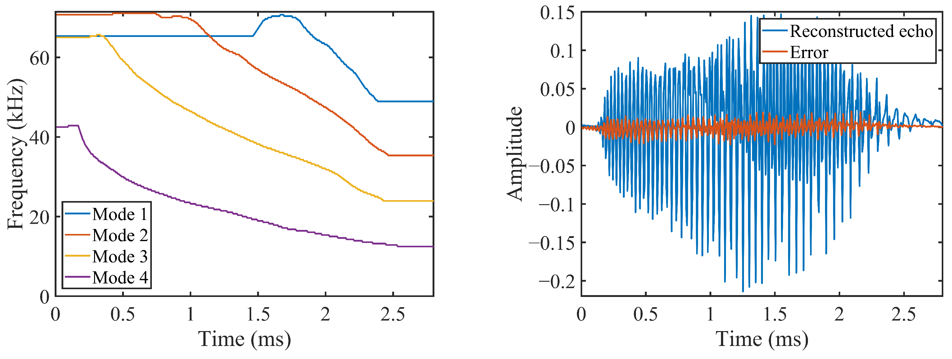
5.3. Application to Bat Echo

We used the bat echo [20] collected by Rice University to verify the adaptability of the MSRT proposed in this paper to the actual signal. The sampling rate of the bat echo used is 140 kHz, with a total of 400 sampling points. The waveform and spectrum are shown in Figure 10. It is not easy to understand how bats use their echoes to identify and locate targets.

Figure 11a shows the STFT of the bat echo. The nonlinear behaviors of bat echolocation precisely in the time–frequency domain are evident. The echo contains four modes, and the duration and frequency of each mode are easily available from the TFR. Figure 11b–e show the zooms of the STFT/MSRT/SST2 and SET2, respectively; the STFT has the lowest concentration, and the other three post-processing methods are significantly better than the STFT. The positioning accuracy of the MSRT for the instantaneous frequency of each mode is comparable to that of the SET2, but it introduces less noise.

In Figure 12, the IFs of each mode are estimated from the MSRT using the ridge extraction algorithm (see Figure 12a). Each mode was reconstructed from its TF coefficients. The reconstructed signals of each mode were superimposed to obtain the reconstructed echoes with tiny reconstruction errors, indicating that the MSRT has a good signal reconstruction capability, i.e., reversibility.

5.4. Application to Electromagnetic Calculation Data

When the cone-shaped target was nutated, we verified the proposed algorithm with electromagnetic calculation data. The cone rotation frequency was 1 Hz, and the simulation time was 5 s. The other simulation parameters are shown in Table 2. First, CADFEKO was used to establish the cone-shaped target shown in Figure 13a, and the static echo at full attitude was calculated. According to the Section 2, the field of view angle change law when the target is nutated (see in Figure 13b) was obtained. Then, the static data at the corresponding posture were extracted from the full-pose static echo to form the dynamic echo. In order to avoid the influence of the occlusion effect on the scattering intensity, the amplitude of the echo signal was normalized, that is $S_n\left(t\right)=S\left(t\right)/\left|S\left(t\right)\right|$. The short-time Fourier transform and MSRT were obtained as shown in Figure 13c,d, respectively, and it can be seen that the C scattering center is in an occluded state, which is consistent with the theoretical analysis. The MSRT has a higher time–frequency energy concentration. Figure 13e,f show that the proposed algorithm can extract the complete micro-Doppler curves corresponding to A and B and achieve the correct correlation.

For more complex objects, the radar echo behaves as a multi-component signal. The proposed algorithm obtains the TFR of the echo through the MSRT, and the ridge segment linking is used to associate and reorganize the ridges of each mode. As long as the various modes of the target echo signal do not completely overlap in the time–frequency domain, that is the requirements of separability are met [17], the algorithm is still applicable.

6. Conclusions

Aiming at the problems of the low precision of separation curves and easy association errors of overlapping m-D curves in the existing methods, we proposed an m-D curve separation algorithm with a space target based on the MSRT and ridge segment linking. Based on the idea of the SRT, the second-order frequency estimation operator is introduced to correct the SRT, which assists in rearranging the time–frequency coefficients of strongly time-varying signals. The MSRT can obtain a relatively high time–frequency concentration, strong noise robustness, and low computational complexity. Then, the m-D curve of the target scattering center is extracted from the MSRT, and the position of the cross-interval is adaptively determined according to the distance of each scattering center at each moment. Then, the m-D curve segments are correlated and reorganized by ridge segment linking. The simulation and experimental results verify the effectiveness of the algorithm. When the signal is completely submerged in noise, the denoising method of the radar signal or the more robust TFA method can improve the effectiveness of the proposed algorithm.

References

1. Chen, V.; Li, F.; Ho, S.S.; Wechsler, H. Micro-Doppler effect in radar: Phenomenon, model, and simulation study. IEEE Trans. Aerosp. Electron. Syst. 2006, 42, 2–21. [Google Scholar] [CrossRef]
2. Tian, X.; Bai, X.; Xue, R.; Qin, R.; Zhou, F. Fusion Recognition of Space Targets with Micro-Motion. IEEE Trans. Aerosp. Electron. Syst. 2022. [Google Scholar] [CrossRef]
3. Chen, J.; Zhang, J.; Jin, Y.; Yu, H.; Liang, B.; Yang, D.G. Real-Time Processing of Spaceborne SAR Data With Nonlinear Trajectory Based on Variable PRF. IEEE Trans. Geosci. Remote Sens. 2022, 60, 5205212. [Google Scholar] [CrossRef]
4. Li, G.; Varshney, P.K. Micro-Doppler parameter estimation via parametric sparse representation and pruned orthogonal matching pursuit. IEEE J. Sel. Top. Appl. Earth Obs. Remote Sens. 2014, 7, 4937–4948. [Google Scholar] [CrossRef]
5. Zhao, Y.; Su, Y. The extraction of micro-Doppler signal with EMD algorithm for radar-based small UAVs’ detection. IEEE Trans. Instrum. Meas. 2019, 69, 929–940. [Google Scholar] [CrossRef]
6. Wang, Z.; Luo, Y.; Li, K.; Yuan, H.; Zhang, Q. Micro-Doppler Parameters Extraction of Precession Cone-Shaped Targets Based on Rotating Antenna. Remote Sens. 2022, 14, 2549. [Google Scholar] [CrossRef]
7. Zhu, N.; Hu, J.; Xu, S.; Wu, W.; Zhang, Y.; Chen, Z. Micro-Motion Parameter Extraction for Ballistic Missile with Wideband Radar Using Improved Ensemble EMD Method. Remote Sens. 2021, 13, 3545. [Google Scholar] [CrossRef]
8. Zhang, W.; Xie, J.; Li, H. Micro-Doppler separation method in ISAR imaging based on short-time chirplet decomposition. J. Appl. Remote Sens. 2021, 15, 036515. [Google Scholar] [CrossRef]
9. Choi, I.; Kang, K.; Kim, K.; Park, S. Use of ICA to Separate Micro-Doppler Signatures in ISAR Images of Aircraft That Has Fast-Rotating Parts. IEEE Trans. Aerosp. Electron. Syst. 2022, 58, 234–246. [Google Scholar] [CrossRef]
10. Djurović, I.; Stanković, L. An algorithm for the Wigner distribution based instantaneous frequency estimation in a high noise environment. Signal Process. 2004, 84, 631–643. [Google Scholar] [CrossRef]
11. Djurović, I.; Popović-Bugarin, V.; Simeunović, M. The STFT-based estimator of micro-Doppler parameters. IEEE Trans. Aerosp. Electron. Syst. 2017, 53, 1273–1283. [Google Scholar] [CrossRef]
12. Li, B.; Zhang, Z.; Zhu, X. Adaptive S-Transform with Chirp-Modulated Window and Its Synchroextracting Transform. Circuits Syst. Signal Process. 2021, 40, 5654–5681. [Google Scholar] [CrossRef]
13. Pang, C.; Han, Y.; Hou, H.; Liu, S.; Zhang, N. Micro-Doppler Signal Time-Frequency Algorithm Based on STFRFT. Sensors 2016, 16, 1559. [Google Scholar] [CrossRef] [PubMed]
14. Boashash, B.; Black, P. An efficient real-time implementation of the Wigner-Ville distribution. IEEE Trans. Acoust. Speech Signal Process. 1987, 35, 1611–1618. [Google Scholar] [CrossRef]
15. Yang, Y.; Peng, Z.; Zhang, W.; Meng, G. Parameterised time–frequency analysis methods and their engineering applications: A review of recent advances. Mech. Syst. Signal Process. 2019, 119, 182–221. [Google Scholar] [CrossRef]
16. Ai, X.; Xu, Z.; Wu, Q.; Liu, X.; Xiao, S. Parametric Representation and Application of Micro-Doppler Characteristics for Cone-Shaped Space Targets. IEEE Sens. J. 2019, 19, 11839–11849. [Google Scholar] [CrossRef]
17. Meignen, S.; Pham, D.H.; McLaughlin, S. On demodulation, ridge detection, and synchrosqueezing for multicomponent signals. IEEE Trans. Signal Process. 2017, 65, 2093–2103. [Google Scholar] [CrossRef] [Green Version]
18. Pan, P.; Zhang, Y.; Deng, Z.; Fan, S.; Huang, X. TFA-Net: A Deep Learning-Based Time-Frequency Analysis Tool. IEEE Trans. Neural Netw. Learn. Syst. 2022. [Google Scholar] [CrossRef]
19. Meignen, S.; Singh, N. Analysis of Reassignment Operators Used in Synchrosqueezing Transforms: With an Application to Instantaneous Frequency Estimation. IEEE Trans. Signal Process. 2021, 70, 216–227. [Google Scholar] [CrossRef]
20. Oberlin, T.; Meignen, S.; Perrier, V. Second-Order Synchrosqueezing Transform or Invertible Reassignment? Towards Ideal Time-Frequency Representations. IEEE Trans. Signal Process. 2015, 63, 1335–1344. [Google Scholar] [CrossRef] [Green Version]
21. Yu, G.; Yu, M.; Xu, C. Synchroextracting transform. IEEE Trans. Ind. Electron. 2017, 64, 8042–8054. [Google Scholar] [CrossRef]
22. Bao, W.; Li, F.; Tu, X.; Hu, Y.; He, Z. Second-order synchroextracting transform with application to fault diagnosis. IEEE Trans. Instrum. Meas. 2020, 70, 3509409. [Google Scholar] [CrossRef]
23. Pham, D.H.; Meignen, S. High-Order Synchrosqueezing Transform for Multicomponent Signals Analysis—With an Application to Gravitational-Wave Signal. IEEE Trans. Signal Process. 2017, 65, 3168–3178. [Google Scholar] [CrossRef] [Green Version]
24. Li, M.; Wang, T.; Kong, Y.; Chu, F. Synchro-reassigning transform for instantaneous frequency estimation and signal reconstruction. IEEE Trans. Ind. Electron. 2021, 69, 7263–7274. [Google Scholar] [CrossRef]
25. McAulay, R.; Quatieri, T. Speech analysis/synthesis based on a sinusoidal representation. IEEE Trans. Acoust. Speech Signal Process. 1986, 34, 744–754. [Google Scholar] [CrossRef] [Green Version]
26. Rankine, L.; Mesbah, M.; Boashash, B. IF estimation for multicomponent signals using image processing techniques in the time–frequency domain. Signal Process. 2007, 87, 1234–1250. [Google Scholar] [CrossRef] [Green Version]
27. Ren, K.; Du, L.; Lu, X.; Zhuo, Z.; Li, L. Instantaneous Frequency Estimation Based on Modified Kalman Filter for Cone-Shaped Target. Remote Sens. 2020, 12, 2766. [Google Scholar] [CrossRef]
28. Hong, L.; Wang, X.; Liu, S. Micro-Doppler curves extraction based on high-order particle filter track-before detect. IEEE Geosci. Remote Sens. Lett. 2019, 16, 1550–1554. [Google Scholar] [CrossRef]
29. Zhu, N.; Xu, S.; Li, C.; Hu, J.; Fan, X.; Wu, W.; Chen, Z. An Improved Phase-Derived Range Method Based on High-Order Multi-Frame Track-Before-Detect for Warhead Detection. Remote Sens. 2022, 14, 29. [Google Scholar] [CrossRef]
30. Chen, S.; Dong, X.; Xing, G.; Peng, Z.; Zhang, W.; Meng, G. Separation of overlapped non-stationary signals by ridge path regrouping and intrinsic chirp component decomposition. IEEE Sens. J. 2017, 17, 5994–6005. [Google Scholar] [CrossRef]
31. Barbarossa, S. Analysis of multicomponent LFM signals by a combined Wigner-Hough transform. IEEE Trans. Signal Process. 1995, 43, 1511–1515. [Google Scholar] [CrossRef]
32. Ding, Y.; Liu, R.; She, Y.; Jin, B.; Peng, Y. Micro-Doppler Trajectory Estimation of Human Movers by Viterbi–Hough Joint Algorithm. IEEE Trans. Geosci. Remote Sens. 2022, 60, 5113111. [Google Scholar] [CrossRef]
33. Zhou, Y.; Chen, Z.; Zhang, L.; Xiao, J. Micro-Doppler Curves Extraction and Parameters Estimation for Cone-Shaped Target with Occlusion Effect. IEEE Sens. J. 2018, 18, 2892–2902. [Google Scholar] [CrossRef]
34. Shi, Y.; Jiu, B.; Liu, H. Optimization-Based Discontinuous Observation Strategy for Micro-Doppler Signature Extraction of Space Cone Targets. IEEE Access 2019, 7, 58915–58929. [Google Scholar] [CrossRef]
35. Chen, J.; Xing, M.; Yu, H.; Liang, B.; Peng, J.; Sun, G.C. Motion Compensation/Autofocus in Airborne Synthetic Aperture Radar: A Review. IEEE Geosci. Remote Sens. Mag. 2022, 10, 185–206. [Google Scholar] [CrossRef]
Figure 1. Micro-motion model of cone target with three scattering centers A, B and C.
Remotesensing 14 03691 g001
Figure 2. Ridge-segment linking process. (a) Determine the intersection interval. (b) Calculate the rate of change of the ridges. (c) Ridge-segment linking.
Remotesensing 14 03691 g002
Figure 3. Detection scene and signal processing flow. (a) Detection scene of space target with three scattering centers A, B and C. (b) Processing flow.
Remotesensing 14 03691 g003
Figure 4. Target model and TFD. (a) A flat-bottomed cone-shaped target with a rotationally symmetric structure. A, B and C are the three scattering centers of the cone-shaped target. (b) STFT result.
Remotesensing 14 03691 g004
Figure 5. Micro-Doppler spectrum through different time–frequency analysis methods. (a) SST. (b) SET. (c) SRT. (d) SST2. (e) SET2. (f) MSRT.
Remotesensing 14 03691 g005
Figure 6. Ridge detection and mode reconstruction results. (a) Ridge detection result. (b) Ridge segment linking. (c) Mode reconstruction result of scatter A. (d) Mode reconstruction result of scatter B.
Remotesensing 14 03691 g006
Figure 7. IF estimates and errors. (a) The instantaneous frequency estimate of the scatter A by different TFAs. (b) IF estimation error.
Remotesensing 14 03691 g007
Figure 8. Ridge correlation results by different methods. (ac) Result of ridge segment linking, the RPRG, and the Viterbi algorithm for a two-component signal. (df) Result of ridge segment linking, the RPRG, and the Viterbi algorithm for a three-component signal.
Remotesensing 14 03691 g008
Figure 9. Noise robustness verification results of the MSRT. (a) Rényi entropy under different SNR conditions. (b) Output SNR of reconstruction results under different SNR conditions.
Remotesensing 14 03691 g009
Figure 10. The base information of the bat signal. (a) Waveform. (b) Spectrum.
Remotesensing 14 03691 g010
Figure 11. Results of different TFAs. (a) STFT result. (b) Zoom of the STFT result. (c) Zoom of the MSRT result. (d) Zoom of the SST2 result. (e) Zoom of the SET2 result.
Remotesensing 14 03691 g011
Figure 12. The estimated IF and mode reconstruction of bat echo. (a) The estimated IF trajectories based on the MSRT. (b) Mode reconstruction results and error.
Remotesensing 14 03691 g012
Figure 13. Results of the proposed algorithm on electromagnetic computational data. (a) Cone-shaped target model with three scattering centers. (b) The field of view angle change law. (c) Result by the STFT. (d) Result by the MSRT. (e) Ridge extraction. (f) Ridge segment linking.
Remotesensing 14 03691 g013aRemotesensing 14 03691 g013b