
Linear and Non-Linear Vegetation Trend Analysis throughout Iran Using Two Decades of MODIS NDVI Imagery


Abstract
:1. Introduction
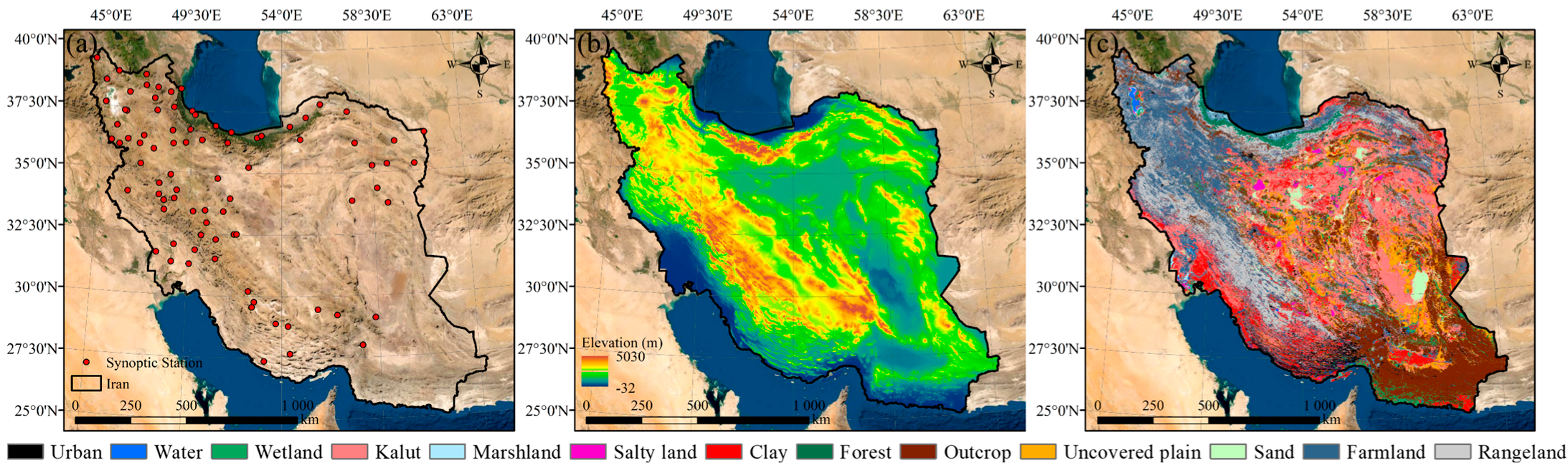
2. Study Area
3. Material and Methods
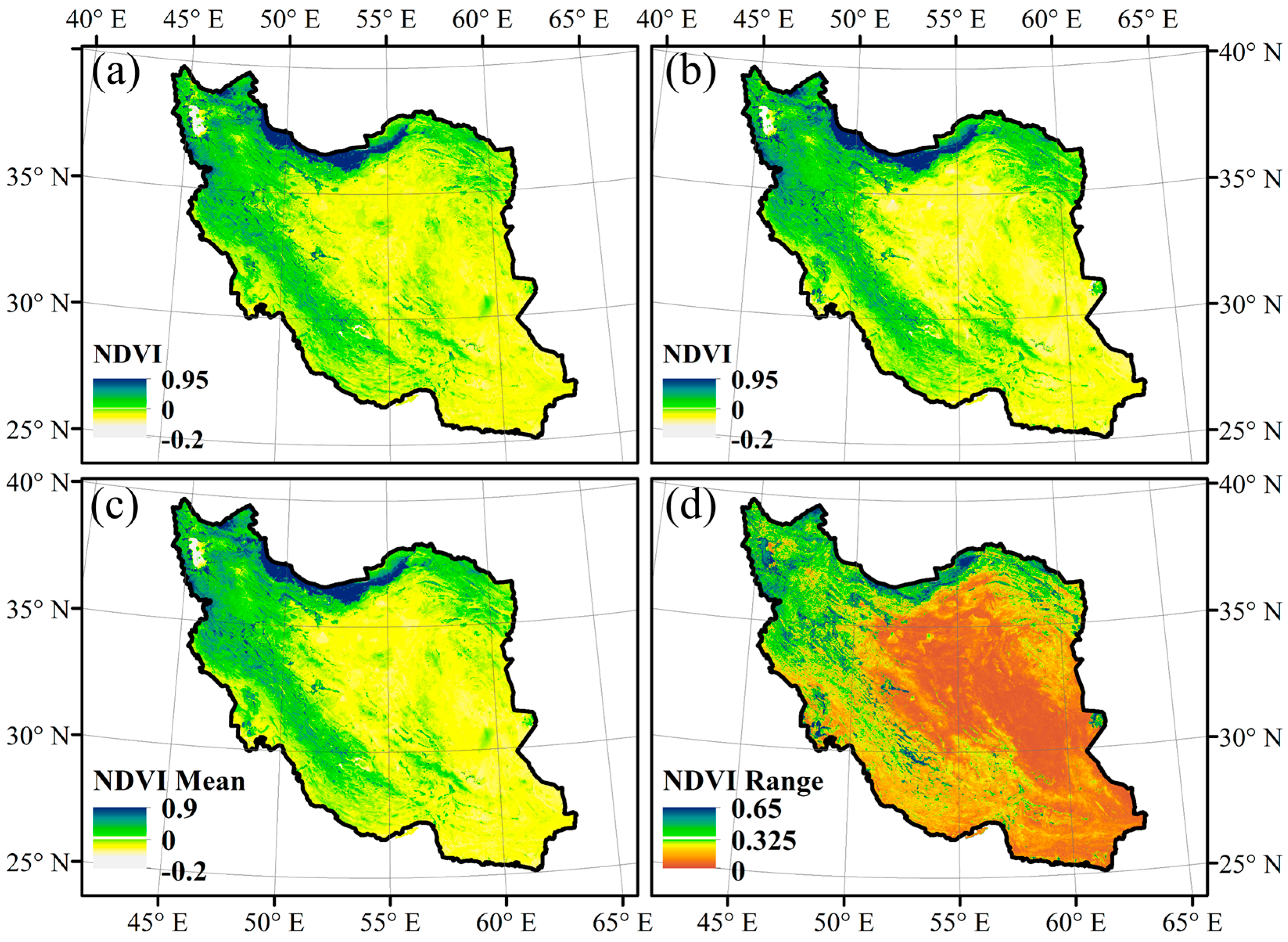
3.1. NDVI Dataset
3.2. Land Cover Dataset
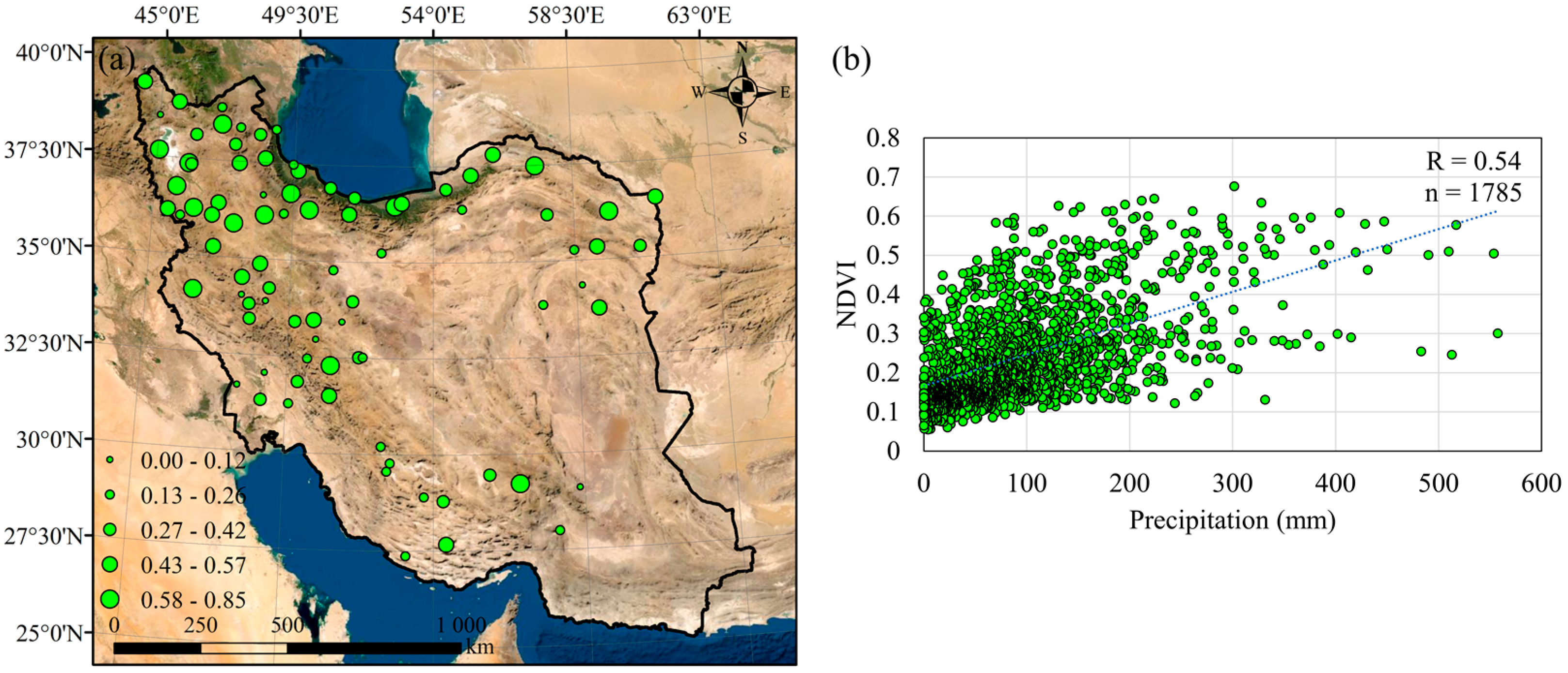
3.3. In-Situ Precipitation Dataset
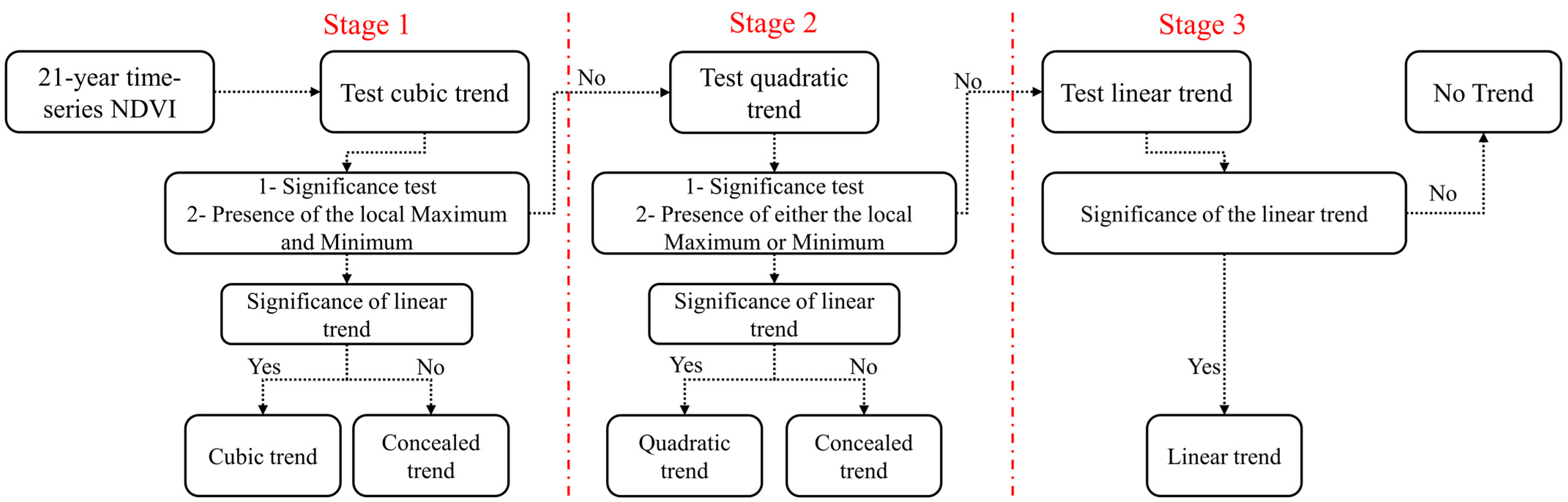
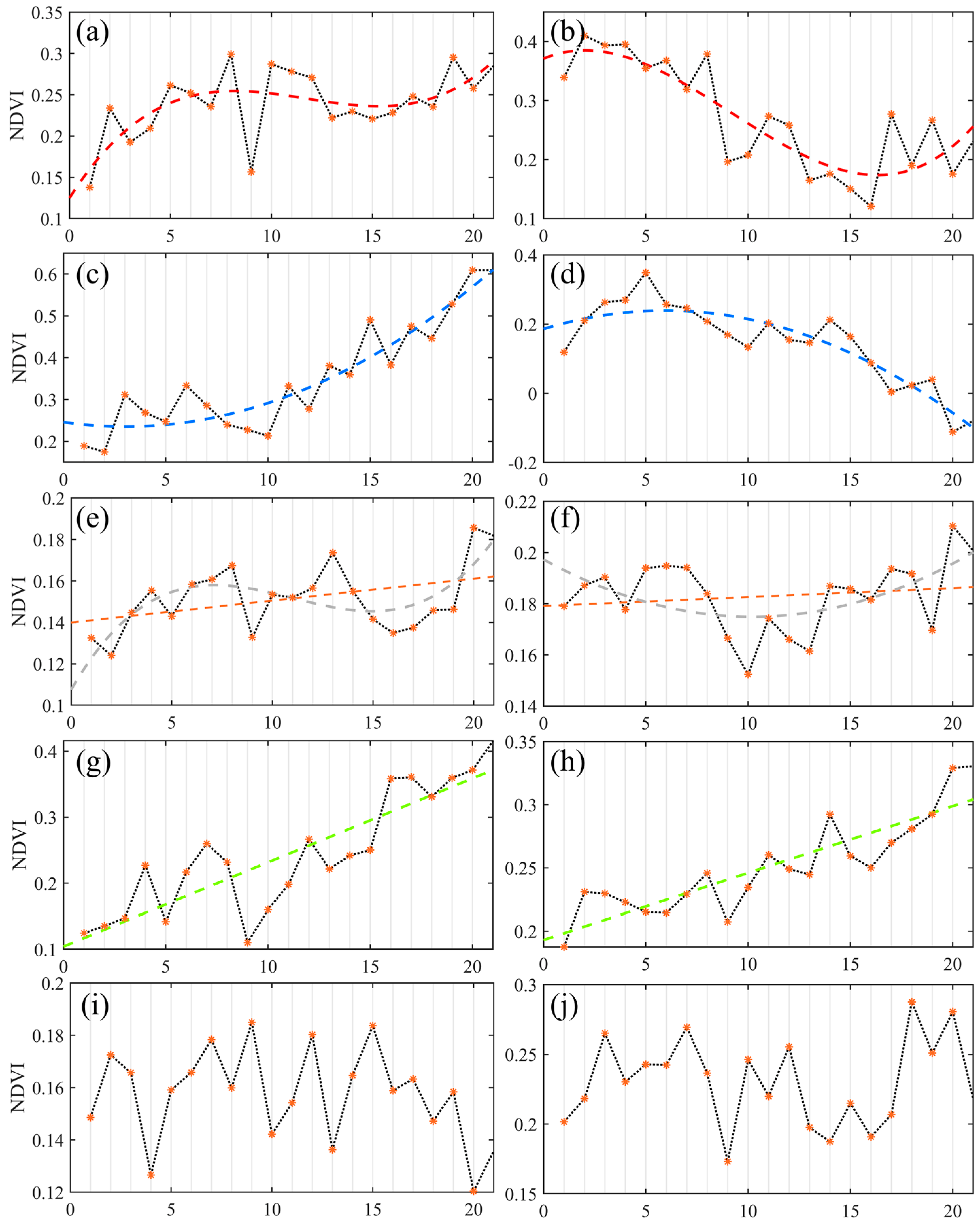
3.4. Linear and Non-Linear Trend Analysis
4. Results
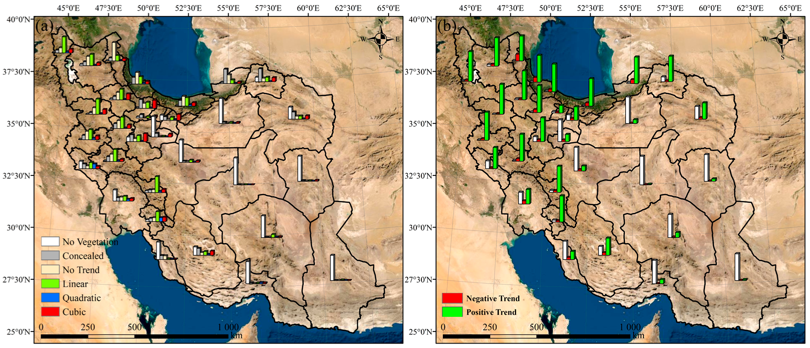
4.1. Trend Linearity/Non-Linearity Assessment
4.2. Trend Analysis
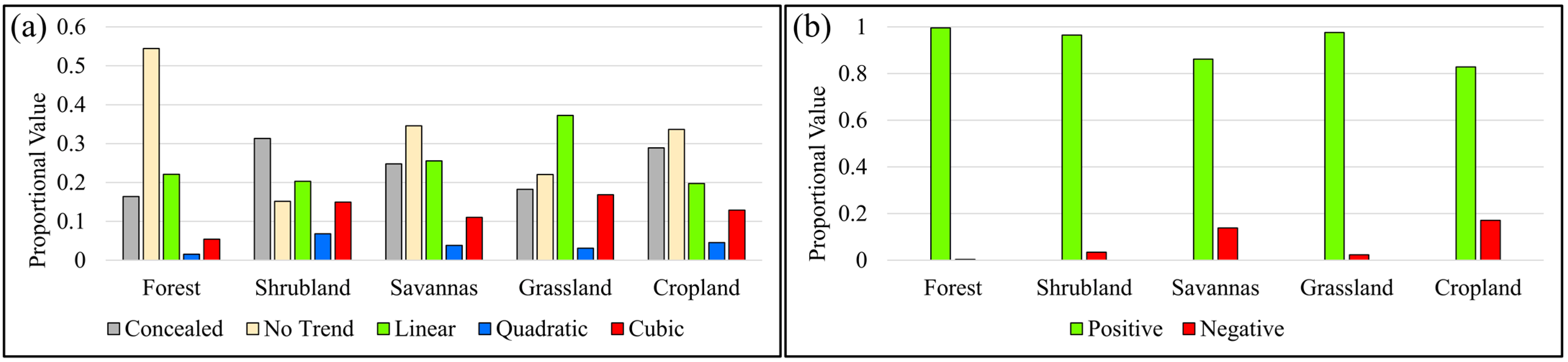
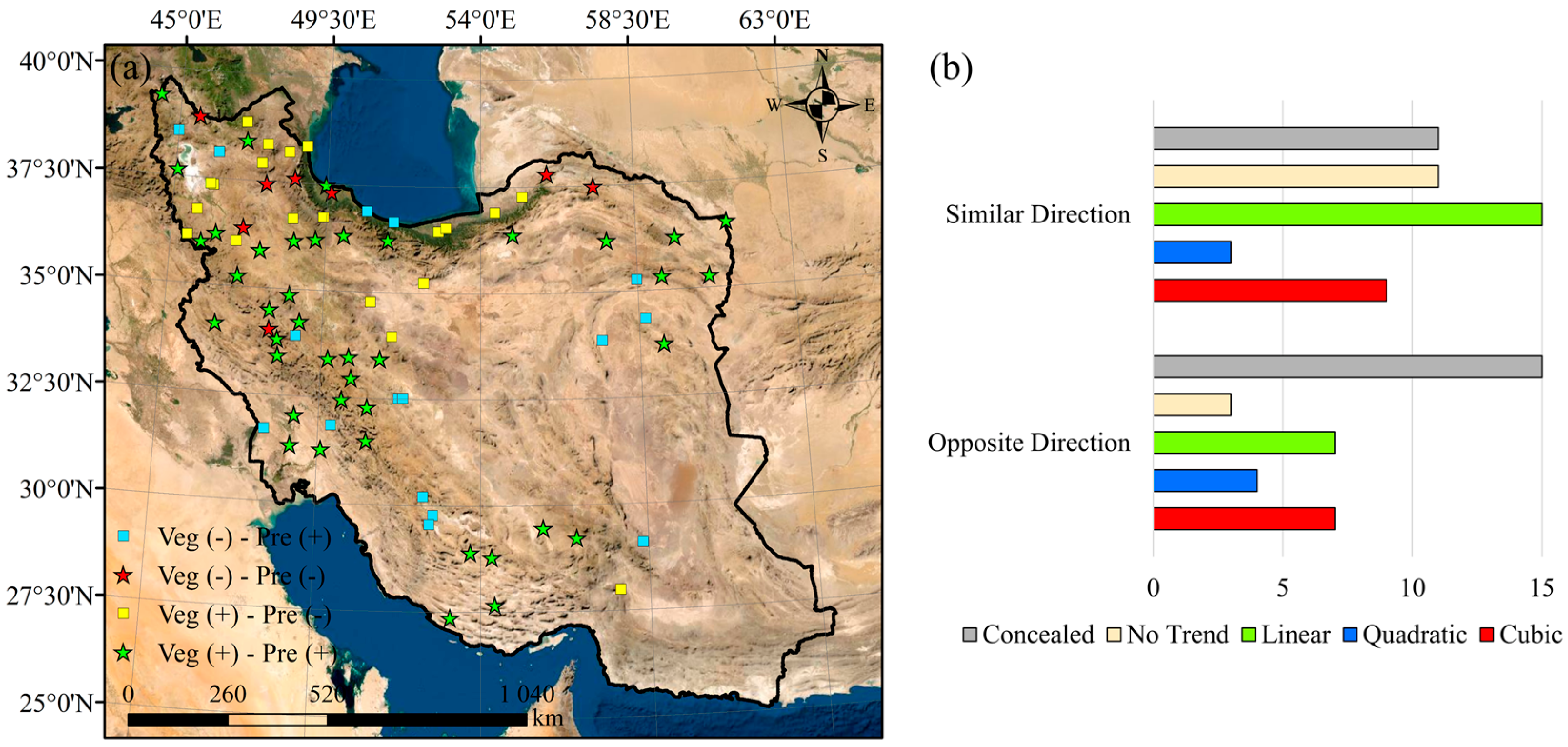
4.3. Vegetation Trend vs. Land Cover and Precipitation
5. Discussion
6. Conclusions
Author Contributions
Funding
Data Availability Statement
Acknowledgments
Conflicts of Interest
References
- Zhang, Y.; Song, C.; Band, L.E.; Sun, G.; Li, J. Reanalysis of Global Terrestrial Vegetation Trends from MODIS Products: Browning or Greening? Remote Sens. Environ. 2017, 191, 145–155. [Google Scholar] [CrossRef] [Green Version]
- Ruan, Z.; Kuang, Y.; He, Y.; Zhen, W.; Ding, S. Detecting Vegetation Change in the Pearl River Delta Region Based on Time Series Segmentation and Residual Trend Analysis (TSS-RESTREND) and MODIS NDVI. Remote Sens. 2020, 12, 4049. [Google Scholar] [CrossRef]
- Pakeman, R.J.; Fielding, D.A.; Everts, L.; Littlewood, N.A. Long-Term Impacts of Changed Grazing Regimes on the Vegetation of Heterogeneous Upland Grasslands. J. Appl. Ecol. 2019, 56, 1794–1805. [Google Scholar] [CrossRef]
- Pan, N.; Feng, X.; Fu, B.; Wang, S.; Ji, F.; Pan, S. Increasing Global Vegetation Browning Hidden in Overall Vegetation Greening: Insights from Time-Varying Trends. Remote Sens. Environ. 2018, 214, 59–72. [Google Scholar] [CrossRef]
- Chen, C.; Park, T.; Wang, X.; Piao, S.; Xu, B.; Chaturvedi, R.K.; Fuchs, R.; Brovkin, V.; Ciais, P.; Fensholt, R.; et al. China and India Lead in Greening of the World through Land-Use Management. Nat. Sustain. 2019, 2, 122–129. [Google Scholar] [CrossRef] [PubMed]
- Chu, H.; Venevsky, S.; Wu, C.; Wang, M. NDVI-Based Vegetation Dynamics and Its Response to Climate Changes at Amur-Heilongjiang River Basin from 1982 to 2015. Sci. Total Environ. 2019, 650, 2051–2062. [Google Scholar] [CrossRef] [PubMed]
- Yang, Y.; Wang, S.; Bai, X.; Tan, Q.; Li, Q.; Wu, L.; Tian, S.; Hu, Z.; Li, C.; Deng, Y. Factors Affecting Long-Term Trends in Global NDVI. Forests 2019, 10, 372. [Google Scholar] [CrossRef] [Green Version]
- Sun, Q.; Miao, C.; Duan, Q.; Ashouri, H.; Sorooshian, S.; Hsu, K.-L. A Review of Global Precipitation Data Sets: Data Sources, Estimation, and Intercomparisons. Rev. Geophys. 2018, 56, 79–107. [Google Scholar] [CrossRef] [Green Version]
- Gajewski, K. Impact of Holocene Climate Variability on Arctic Vegetation. Glob. Planet. Chang. 2015, 133, 272–287. [Google Scholar] [CrossRef] [Green Version]
- Kazemzadeh, M.; Noori, Z.; Alipour, H.; Jamali, S.; Seyednasrollah, B. Natural and Anthropogenic Forcings Lead to Contrasting Vegetation Response in Long-Term vs. Short-Term Timeframes. J. Environ. Manag. 2021, 286, 112249. [Google Scholar] [CrossRef]
- Dubovyk, O.; Landmann, T.; Erasmus, B.F.N.; Tewes, A.; Schellberg, J. Monitoring Vegetation Dynamics with Medium Resolution MODIS-EVI Time Series at Sub-Regional Scale in Southern Africa. Int. J. Appl. Earth Obs. Geoinf. 2015, 38, 175–183. [Google Scholar] [CrossRef]
- Kim, J.Y.; Rastogi, G.; Do, Y.; Kim, D.-K.; Muduli, P.R.; Samal, R.N.; Pattnaik, A.K.; Joo, G.-J. Trends in a Satellite-Derived Vegetation Index and Environmental Variables in a Restored Brackish Lagoon. Glob. Ecol. Conserv. 2015, 4, 614–624. [Google Scholar] [CrossRef] [Green Version]
- Wang, J.; Xie, Y.; Wang, X.; Dong, J.; Bie, Q. Detecting Patterns of Vegetation Gradual Changes (2001–2017) in Shiyang River Basin, Based on a Novel Framework. Remote Sens. 2019, 11, 2475. [Google Scholar] [CrossRef] [Green Version]
- Jiang, W.; Yuan, L.; Wang, W.; Cao, R.; Zhang, Y.; Shen, W. Spatio-Temporal Analysis of Vegetation Variation in the Yellow River Basin. Ecol. Indic. 2015, 51, 117–126. [Google Scholar] [CrossRef]
- Huang, S.; Tang, L.; Hupy, J.P.; Wang, Y.; Shao, G. A Commentary Review on the Use of Normalized Difference Vegetation Index (NDVI) in the Era of Popular Remote Sensing. J. For. Res. 2021, 32, 1–6. [Google Scholar] [CrossRef]
- Eckert, S.; Hüsler, F.; Liniger, H.; Hodel, E. Trend Analysis of MODIS NDVI Time Series for Detecting Land Degradation and Regeneration in Mongolia. J. Arid Environ. 2015, 113, 16–28. [Google Scholar] [CrossRef]
- Zhang, Y.; Ye, A. Spatial and Temporal Variations in Vegetation Coverage Observed Using AVHRR GIMMS and Terra MODIS Data in the Mainland of China. Int. J. Remote Sens. 2020, 41, 4238–4268. [Google Scholar] [CrossRef]
- Fensholt, R.; Langanke, T.; Rasmussen, K.; Reenberg, A.; Prince, S.D.; Tucker, C.; Scholes, R.J.; Le, Q.B.; Bondeau, A.; Eastman, R.; et al. Greenness in Semi-Arid Areas across the Globe 1981–2007—An Earth Observing Satellite Based Analysis of Trends and Drivers. Remote Sens. Environ. 2012, 121, 144–158. [Google Scholar] [CrossRef]
- Bruzzone, O.; Easdale, M.H. Rhythm of Change of Trend-Cycles of Vegetation Dynamics as an Early Warning Indicator for Land Management. Ecol. Indic. 2021, 126, 107663. [Google Scholar] [CrossRef]
- Huete, A.R. A Soil-Adjusted Vegetation Index (SAVI). Remote Sens. Environ. 1988, 25, 295–309. [Google Scholar] [CrossRef]
- Xue, J.; Su, B. Significant Remote Sensing Vegetation Indices: A Review of Developments and Applications. J. Sens. 2017, 2017, 1353691. [Google Scholar] [CrossRef] [Green Version]
- Rouse, J.W.; Haas, R.H.; Schell, J.A.; Deering, D.W. Monitoring vegetation system in the great plains with ERTS. In Proceedings of the Third Earth Resources Technology Satellite-1 Symposium, Greenbelt, MD, USA, 1 January 1974; pp. 3010–3017, NASA SP-351. [Google Scholar]
- Seydi, S.T.; Amani, M.; Ghorbanian, A. A Dual Attention Convolutional Neural Network for Crop Classification Using Time-Series Sentinel-2 Imagery. Remote Sens. 2022, 14, 498. [Google Scholar] [CrossRef]
- Amani, M.; Mahdavi, S.; Kakooei, M.; Ghorbanian, A.; Brisco, B.; Delancey, E.; Toure, S.; Reyes, E.L. Wetland Change Analysis in Alberta, Canada Using Four Decades of Landsat Imagery. IEEE J. Sel. Top. Appl. Earth Obs. Remote Sens. 2021, 14, 10314–10335. [Google Scholar] [CrossRef]
- Petersen, L.K. Real-Time Prediction of Crop Yields from MODIS Relative Vegetation Health: A Continent-Wide Analysis of Africa. Remote Sens. 2018, 10, 1726. [Google Scholar] [CrossRef] [Green Version]
- Karan, S.K.; Samadder, S.R.; Maiti, S.K. Assessment of the Capability of Remote Sensing and GIS Techniques for Monitoring Reclamation Success in Coal Mine Degraded Lands. J. Environ. Manag. 2016, 182, 272–283. [Google Scholar] [CrossRef]
- Yan, J.; Zhang, G.; Ling, H.; Han, F. Comparison of Time-Integrated NDVI and Annual Maximum NDVI for Assessing Grassland Dynamics. Ecol. Indic. 2022, 136, 108611. [Google Scholar] [CrossRef]
- Zhang, Y.; He, Y.; Li, Y.; Jia, L. Spatiotemporal Variation and Driving Forces of NDVI from 1982 to 2015 in the Qinba Mountains, China. Environ. Sci. Pollut. Res. 2022, 29, 52277–52288. [Google Scholar] [CrossRef]
- Gao, W.; Zheng, C.; Liu, X.; Lu, Y.; Chen, Y.; Wei, Y.; Ma, Y. NDVI-Based Vegetation Dynamics and Their Responses to Climate Change and Human Activities from 1982 to 2020: A Case Study in the Mu Us Sandy Land, China. Ecol. Indic. 2022, 137, 108745. [Google Scholar] [CrossRef]
- Huete, A.; Didan, K.; Miura, T.; Rodriguez, E.P.; Gao, X.; Ferreira, L.G. Overview of the Radiometric and Biophysical Performance of the MODIS Vegetation Indices. Remote Sens. Environ. 2002, 83, 195–213. [Google Scholar] [CrossRef]
- Matsushita, B.; Yang, W.; Chen, J.; Onda, Y.; Qiu, G. Sensitivity of the Enhanced Vegetation Index (EVI) and Normalized Difference Vegetation Index (NDVI) to Topographic Effects: A Case Study in High-Density Cypress Forest. Sensors 2007, 7, 2636–2651. [Google Scholar] [CrossRef] [Green Version]
- Didan, K.; Munoz, A.B.; Solano, R.; Huete, A. MODIS Vegetation Index User’s Guide (MOD13 Series); Vegetation Index and Phenology Lab, University of Arizona: Tucson, AZ, USA, 2015. [Google Scholar]
- Kumari, N.; Srivastava, A.; Dumka, U.C. A Long-Term Spatiotemporal Analysis of Vegetation Greenness over the Himalayan Region Using Google Earth Engine. Climate 2021, 9, 109. [Google Scholar] [CrossRef]
- Jamali, S.; Seaquist, J.; Eklundh, L.; Ardö, J. Automated Mapping of Vegetation Trends with Polynomials Using NDVI Imagery over the Sahel. Remote Sens. Environ. 2014, 141, 79–89. [Google Scholar] [CrossRef]
- Liu, C.; Huang, H.; Sun, F. A Pixel-Based Vegetation Greenness Trend Analysis over the Russian Tundra with All Available Landsat Data from 1984 to 2018. Remote Sens. 2021, 13, 4933. [Google Scholar] [CrossRef]
- Sen, P.K. Estimates of the Regression Coefficient Based on Kendall’s Tau. J. Am. Stat. Assoc. 1968, 63, 1379–1389. [Google Scholar] [CrossRef]
- Emamian, A.; Rashki, A.; Kaskaoutis, D.G.; Gholami, A.; Opp, C.; Middleton, N. Assessing Vegetation Restoration Potential under Different Land Uses and Climatic Classes in Northeast Iran. Ecol. Indic. 2021, 122, 107325. [Google Scholar] [CrossRef]
- Gholamnia, M.; Khandan, R.; Bonafoni, S.; Sadeghi, A. Spatiotemporal Analysis of MODIS NDVI in the Semi-Arid Region of Kurdistan (Iran). Remote Sens. 2019, 11, 1723. [Google Scholar] [CrossRef] [Green Version]
- Verbesselt, J.; Hyndman, R.; Newnham, G.; Culvenor, D. Detecting Trend and Seasonal Changes in Satellite Image Time Series. Remote Sens. Environ. 2010, 114, 106–115. [Google Scholar] [CrossRef]
- Sedighifar, Z.; Motlagh, M.G.; Halimi, M. Investigating Spatiotemporal Relationship between EVI of the MODIS and Climate Variables in Northern Iran. Int. J. Environ. Sci. Technol. 2020, 17, 733–744. [Google Scholar] [CrossRef]
- Eskandari Dameneh, H.; Gholami, H.; Telfer, M.W.; Comino, J.R.; Collins, A.L.; Jansen, J.D. Desertification of Iran in the Early Twenty-First Century: Assessment Using Climate and Vegetation Indices. Sci. Rep. 2021, 11, 20548. [Google Scholar] [CrossRef] [PubMed]
- Lenton, T.M.; Held, H.; Kriegler, E.; Hall, J.W.; Lucht, W.; Rahmstorf, S.; Schellnhuber, H.J. Tipping Elements in the Earth’s Climate System. Proc. Natl. Acad. Sci. USA 2008, 105, 1786–1793. [Google Scholar] [CrossRef] [Green Version]
- Lambin, E.F.; Geist, H.J.; Lepers, E. Dynamics of Land-Use and Land-Cover Change in Tropical Regions. Annu. Rev. Environ. Resour. 2003, 28, 205–241. [Google Scholar] [CrossRef] [Green Version]
- Barnosky, A.D.; Hadly, E.A.; Bascompte, J.; Berlow, E.L.; Brown, J.H.; Fortelius, M.; Getz, W.M.; Harte, J.; Hastings, A.; Marquet, P.A.; et al. Approaching a State Shift in Earth’s Biosphere. Nature 2012, 486, 52–58. [Google Scholar] [CrossRef] [PubMed]
- Takaku, J.; Tadono, T.; Tsutsui, K. Generation of High Resolution Global Dsm from Alos Prism. ISPRS Ann. Photogramm. Remote Sens. Spat. Inf. Sci. 2014, 2, 243–248. [Google Scholar] [CrossRef] [Green Version]
- Ghorbanian, A.; Kakooei, M.; Amani, M.; Mahdavi, S.; Mohammadzadeh, A.; Hasanlou, M. Improved Land Cover Map of Iran Using Sentinel Imagery within Google Earth Engine and a Novel Automatic Workflow for Land Cover Classification Using Migrated Training Samples. ISPRS J. Photogramm. Remote Sens. 2020, 167, 276–288. [Google Scholar] [CrossRef]
- Mansouri Daneshvar, M.R.; Ebrahimi, M.; Nejadsoleymani, H. An Overview of Climate Change in Iran: Facts and Statistics. Environ. Syst. Res. 2019, 8, 7. [Google Scholar] [CrossRef] [Green Version]
- Fallah, B.; Sodoudi, S.; Russo, E.; Kirchner, I.; Cubasch, U. Towards Modeling the Regional Rainfall Changes over Iran Due to the Climate Forcing of the Past 6000 Years. Quat. Int. 2017, 429, 119–128. [Google Scholar] [CrossRef] [Green Version]
- Justice, C.O.; Townshend, J.R.G.; Vermote, E.F.; Masuoka, E.; Wolfe, R.E.; Saleous, N.; Roy, D.P.; Morisette, J.T. An Overview of MODIS Land Data Processing and Product Status. Remote Sens. Environ. 2002, 83, 3–15. [Google Scholar] [CrossRef]
- Sobrino, J.A.; Julien, Y. Trend Analysis of Global MODIS-Terra Vegetation Indices and Land Surface Temperature between 2000 and 2011. IEEE J. Sel. Top. Appl. Earth Obs. Remote Sens. 2013, 6, 2139–2145. [Google Scholar] [CrossRef]
- Wang, D.; Morton, D.; Masek, J.; Wu, A.; Nagol, J.; Xiong, X.; Levy, R.; Vermote, E.; Wolfe, R. Impact of Sensor Degradation on the MODIS NDVI Time Series. Remote Sens. Environ. 2012, 119, 55–61. [Google Scholar] [CrossRef] [Green Version]
- MOD13Q1 V006. Available online: https://lpdaac.usgs.gov/products/mod13q1v006/ (accessed on 5 April 2022).
- MODIS Validation Strategy. Available online: https://modis-land.gsfc.nasa.gov/MODLAND_val.html?_ga=2.3712953.804892803.1651590227-365777974.1651413819 (accessed on 5 April 2022).
- General Accuracy Statement for Vegetation Indices. Available online: https://modis-land.gsfc.nasa.gov/ValStatus.php?ProductID=MOD13&_ga=2.70272921.804892803.1651590227-365777974.1651413819 (accessed on 5 April 2022).
- Sabziparvar, A.A.; Ghahfarokhi, S.M.M.; Khorasani, H.T. Long-Term Changes of Surface Albedo and Vegetation Indices in North of Iran. Arab. J. Geosci. 2020, 13, 117. [Google Scholar] [CrossRef]
- Ebrahimi-Khusfi, Z.; Mirakbari, M.; Khosroshahi, M. Vegetation Response to Changes in Temperature, Rainfall, and Dust in Arid Environments. Environ. Monit. Assess. 2020, 192, 691. [Google Scholar] [CrossRef]
- Gorelick, N.; Hancher, M.; Dixon, M.; Ilyushchenko, S.; Thau, D.; Moore, R. Google Earth Engine: Planetary-Scale Geospatial Analysis for Everyone. Remote Sens. Environ. 2017, 202, 18–27. [Google Scholar] [CrossRef]
- Amani, M.; Ghorbanian, A.; Ahmadi, S.A.; Kakooei, M.; Moghimi, A.; Mirmazloumi, S.M.; Moghaddam, S.H.A.; Mahdavi, S.; Ghahremanloo, M.; Parsian, S.; et al. Google Earth Engine Cloud Computing Platform for Remote Sensing Big Data Applications: A Comprehensive Review. IEEE J. Sel. Top. Appl. Earth Obs. Remote Sens. 2020, 13, 5326–5350. [Google Scholar] [CrossRef]
- Sulla-Menashe, D.; Gray, J.M.; Abercrombie, S.P.; Friedl, M.A. Hierarchical Mapping of Annual Global Land Cover 2001 to Present: The MODIS Collection 6 Land Cover Product. Remote Sens. Environ. 2019, 222, 183–194. [Google Scholar] [CrossRef]
- Zhao, F.; Wu, Y.; Sivakumar, B.; Long, A.; Qiu, L.; Chen, J.; Wang, L.; Liu, S.; Hu, H. Climatic and Hydrologic Controls on Net Primary Production in a Semiarid Loess Watershed. J. Hydrol. 2019, 568, 803–815. [Google Scholar] [CrossRef]
- Jin, K.; Wang, F.; Zong, Q.; Qin, P.; Liu, C.; Wang, S. Spatiotemporal Differences in Climate Change Impacts on Vegetation Cover in China from 1982 to 2015. Environ. Sci. Pollut. Res. 2022, 29, 10263–10276. [Google Scholar] [CrossRef]
- Jiang, S.; Chen, X.; Smettem, K.; Wang, T. Climate and Land Use Influences on Changing Spatiotemporal Patterns of Mountain Vegetation Cover in Southwest China. Ecol. Indic. 2021, 121, 107193. [Google Scholar] [CrossRef]
- Zheng, K.; Tan, L.; Sun, Y.; Wu, Y.; Duan, Z.; Xu, Y.; Gao, C. Impacts of Climate Change and Anthropogenic Activities on Vegetation Change: Evidence from Typical Areas in China. Ecol. Indic. 2021, 126, 107648. [Google Scholar] [CrossRef]
- Zheng, K.; Wei, J.-Z.; Pei, J.-Y.; Cheng, H.; Zhang, X.-L.; Huang, F.-Q.; Li, F.-M.; Ye, J.-S. Impacts of Climate Change and Human Activities on Grassland Vegetation Variation in the Chinese Loess Plateau. Sci. Total Environ. 2019, 660, 236–244. [Google Scholar] [CrossRef] [PubMed]
- Notaro, M.; Liu, Z.; Gallimore, R.G.; Williams, J.W.; Gutzler, D.S.; Collins, S. Complex Seasonal Cycle of Ecohydrology in the Southwest United States. J. Geophys. Res. Biogeosci. 2010, 115. [Google Scholar] [CrossRef]
- Chen, Z.; Wang, W.; Fu, J. Vegetation Response to Precipitation Anomalies under Different Climatic and Biogeographical Conditions in China. Sci. Rep. 2020, 10, 830. [Google Scholar] [CrossRef] [PubMed] [Green Version]
- Xu, X.; Liu, H.; Jiao, F.; Gong, H.; Lin, Z. Nonlinear Relationship of Greening and Shifts from Greening to Browning in Vegetation with Nature and Human Factors along the Silk Road Economic Belt. Sci. Total Environ. 2021, 766, 142553. [Google Scholar] [CrossRef] [PubMed]
- Holtvoeth, J.; Vogel, H.; Valsecchi, V.; Lindhorst, K.; Schouten, S.; Wagner, B.; Wolff, G.A. Linear and Non-Linear Responses of Vegetation and Soils to Glacial-Interglacial Climate Change in a Mediterranean Refuge. Sci. Rep. 2017, 7, 8121. [Google Scholar] [CrossRef] [PubMed] [Green Version]
- Jeong, S.-J.; Ho, C.-H.; Brown, M.E.; Kug, J.-S.; Piao, S. Browning in Desert Boundaries in Asia in Recent Decades. J. Geophys. Res. Atmos. 2011, 116. [Google Scholar] [CrossRef] [Green Version]
- Yang, Q.; Qin, Z.; Li, W.; Xu, B. Temporal and Spatial Variations of Vegetation Cover in Hulun Buir Grassland of Inner Mongolia, China. Arid Land Res. Manag. 2012, 26, 328–343. [Google Scholar] [CrossRef]
- Eastman, J.R.; Sangermano, F.; Machado, E.A.; Rogan, J.; Anyamba, A. Global Trends in Seasonality of Normalized Difference Vegetation Index (NDVI), 1982–2011. Remote Sens. 2013, 5, 4799–4818. [Google Scholar] [CrossRef] [Green Version]
- Kazemzadeh, M.; Noori, Z.; Jamali, S.; Abdi, A.M. Four Decades of Air Temperature Data over Iran Reveal Linear and Nonlinear Warming. J. Meteorol. Res. 2022, 36. [Google Scholar] [CrossRef]
- Kazemzadeh, M.; Hashemi, H.; Jamali, S.; Uvo, C.B.; Berndtsson, R.; Huffman, G.J. Linear and Nonlinear Trend Analyzes in Global Satellite-Based Precipitation, 1998–2017. Earth’s Future 2021, 9, e2020EF001835. [Google Scholar] [CrossRef]
- Jamali, S.; Klingmyr, D.; Tagesson, T. Global-Scale Patterns and Trends in Tropospheric NO2 Concentrations, 2005–2018. Remote Sens. 2020, 12, 3526. [Google Scholar] [CrossRef]
- Sahadevan, A.S.; Joseph, C.; Gopinath, G.; Ramakrishnan, R.; Gupta, P. Monitoring the Rapid Changes in Mangrove Vegetation of Coastal Urban Environment Using Polynomial Trend Analysis of Temporal Satellite Data. Reg. Stud. Mar. Sci. 2021, 46, 101871. [Google Scholar] [CrossRef]
- Zhang, Y.; Liang, S.; Xiao, Z. Observed Vegetation Greening and Its Relationships with Cropland Changes and Climate in China. Land 2020, 9, 274. [Google Scholar] [CrossRef]
- Ghebrezgabher, M.G.; Yang, T.; Yang, X.; Sereke, T.E. Assessment of NDVI Variations in Responses to Climate Change in the Horn of Africa. Egypt. J. Remote Sens. Sp. Sci. 2020, 23, 249–261. [Google Scholar] [CrossRef]
- Wingate, V.R.; Phinn, S.R.; Kuhn, N. Mapping Precipitation-Corrected NDVI Trends across Namibia. Sci. Total Environ. 2019, 684, 96–112. [Google Scholar] [CrossRef]
- Braswell, B.H.; Schimel, D.S.; Linder, E.; Moore Iii, B. The Response of Global Terrestrial Ecosystems to Interannual Temperature Variability. Science 1997, 278, 870–873. [Google Scholar] [CrossRef]
- Kong, D.; Zhang, Q.; Singh, V.P.; Shi, P. Seasonal Vegetation Response to Climate Change in the Northern Hemisphere (1982–2013). Glob. Planet. Chang. 2017, 148, 1–8. [Google Scholar] [CrossRef] [Green Version]
- Easdale, M.H.; Bruzzone, O.; Mapfumo, P.; Tittonell, P. Phases or Regimes? R Evisiting NDVI Trends as Proxies for Land Degradation. Land Degrad. Dev. 2018, 29, 433–445. [Google Scholar] [CrossRef]
- Zhang, X.; Xiao, X.; Wang, X.; Xu, X.; Chen, B.; Wang, J.; Ma, J.; Zhao, B.; Li, B. Quantifying Expansion and Removal of Spartina Alterniflora on Chongming Island, China, Using Time Series Landsat Images during 1995–2018. Remote Sens. Environ. 2020, 247, 111916. [Google Scholar] [CrossRef]
- Jiang, L.; Liu, Y.; Wu, S.; Yang, C. Analyzing Ecological Environment Change and Associated Driving Factors in China Based on NDVI Time Series Data. Ecol. Indic. 2021, 129, 107933. [Google Scholar] [CrossRef]
- Yuan, Z.; Wang, Y.; Xu, J.; Wu, Z. Effects of Climatic Factors on the Net Primary Productivity in the Source Region of Yangtze River, China. Sci. Rep. 2021, 11, 1376. [Google Scholar] [CrossRef] [PubMed]
- Chen, Y.; Cao, R.; Chen, J.; Liu, L.; Matsushita, B. A Practical Approach to Reconstruct High-Quality Landsat NDVI Time-Series Data by Gap Filling and the Savitzky–Golay Filter. ISPRS J. Photogramm. Remote Sens. 2021, 180, 174–190. [Google Scholar] [CrossRef]
- Dhillon, M.S.; Dahms, T.; Kuebert-Flock, C.; Borg, E.; Conrad, C.; Ullmann, T. Modelling Crop Biomass from Synthetic Remote Sensing Time Series: Example for the DEMMIN Test Site, Germany. Remote Sens. 2020, 12, 1819. [Google Scholar] [CrossRef]
- Khare, S.; Latifi, H.; Khare, S. Vegetation Growth Analysis of Unesco World Heritage Hyrcanian Forests Using Multi-Sensor Optical Remote Sensing Data. Remote Sens. 2021, 13, 3965. [Google Scholar] [CrossRef]
- Dhillon, M.S.; Dahms, T.; Kübert-Flock, C.; Steffan-Dewenter, I.; Zhang, J.; Ullmann, T. Spatiotemporal Fusion Modelling Using STARFM: Examples of Landsat 8 and Sentinel-2 NDVI in Bavaria. Remote Sens. 2022, 14, 677. [Google Scholar] [CrossRef]
- Zhou, Q.; Rover, J.; Brown, J.; Worstell, B.; Howard, D.; Wu, Z.; Gallant, A.L.; Rundquist, B.; Burke, M. Monitoring Landscape Dynamics in Central Us Grasslands with Harmonized Landsat-8 and Sentinel-2 Time Series Data. Remote Sens. 2019, 11, 328. [Google Scholar] [CrossRef] [Green Version]
- Wang, Y.; Zhang, Z.; Chen, X. Quantifying Influences of Natural and Anthropogenic Factors on Vegetation Changes Based on Geodetector: A Case Study in the Poyang Lake Basin, China. Remote Sens. 2021, 13, 5081. [Google Scholar] [CrossRef]
- Xu, X.; Liu, H.; Lin, Z.; Jiao, F.; Gong, H. Relationship of Abrupt Vegetation Change to Climate Change and Ecological Engineering with Multi-Timescale Analysis in the Karst Region, Southwest China. Remote Sens. 2019, 11, 1564. [Google Scholar] [CrossRef] [Green Version]
- Guo, E.; Wang, Y.; Wang, C.; Sun, Z.; Bao, Y.; Mandula, N.; Jirigala, B.; Bao, Y.; Li, H. NDVI Indicates Long-Term Dynamics of Vegetation and Its Driving Forces from Climatic and Anthropogenic Factors in Mongolian Plateau. Remote Sens. 2021, 13, 688. [Google Scholar] [CrossRef]


| Dataset | Sensor | Resolution Spatial | Time Period | Source | |
|---|---|---|---|---|---|
| Type | Name | ||||
| Satellite | NDVI | MODIS (MOD13Q1) | 250 m | 2000–2020 | Google Earth Engine (GEE) |
| Satellite | Land Cover | MODIS (MCD12Q1) | 500 m | 2001 and 2020 | Google Earth Engine (GEE) |
| In-situ | Precipitation | Synoptic Station | - | 2000–2020 | Islamic Republic of Iran Meteorological Organization (IRIMO) |
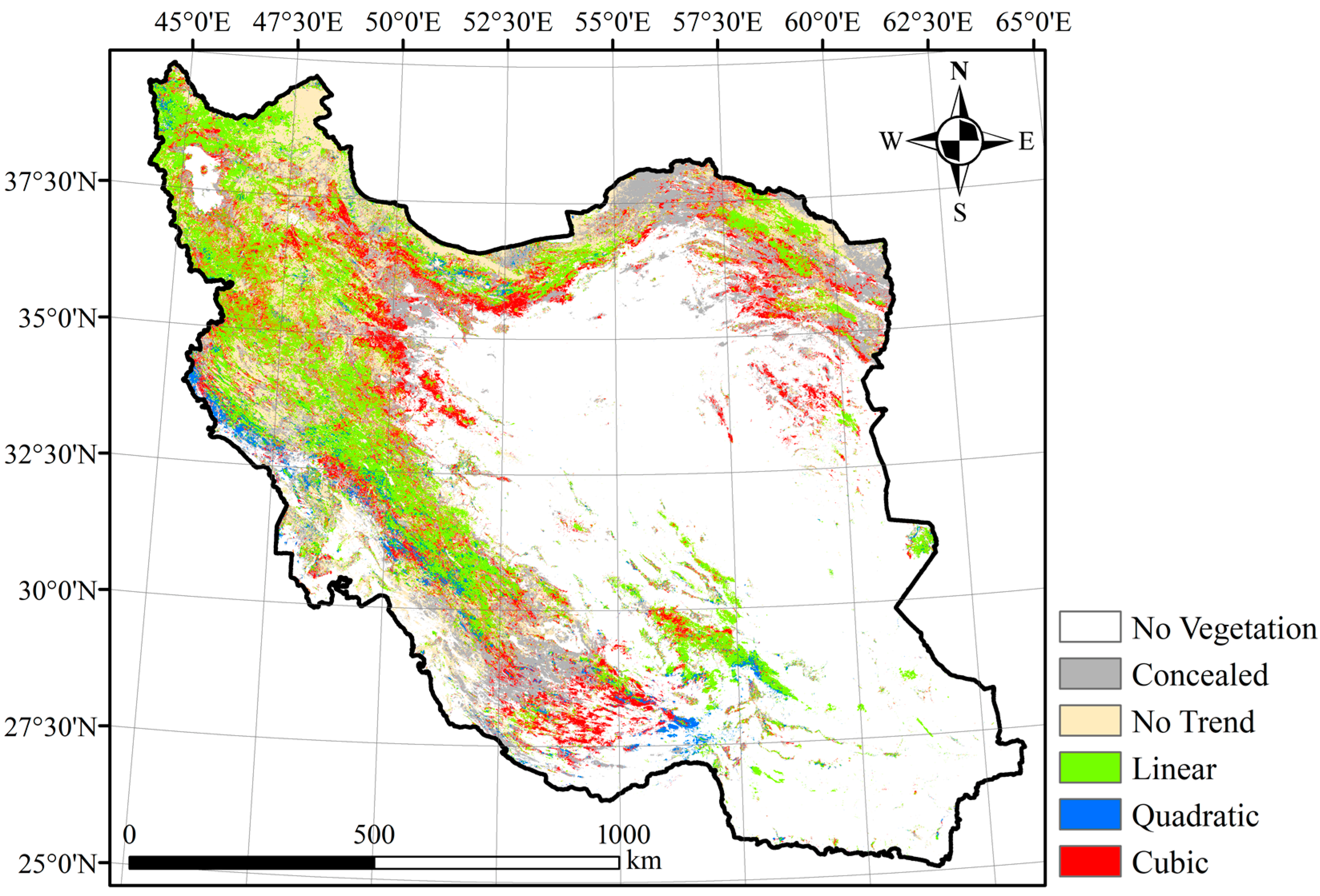
| Trend Type | Pixels (%) | Area (km2) | Positive (km2) | Negative (km2) | Slope Value Range (NDVI Unit) |
|---|---|---|---|---|---|
| No Vegetation | 56 | 1,081,447 | - | - | - |
| Concealed | 11 | 212,622 | 179,181 | 33,608 | −0.016–0.017 |
| No Trend | 9 | 181,929 | 156,042 | 28,273 | −0.013–0.016 |
| Linear | 14 | 270,890 | 258,521 | 6096 | −0.043–0.041 |
| Quadratic | 2 | 38,587 | 39,849 | 3228 | −0.041–0.037 |
| Cubic | 8 | 146,603 | 143,756 | 9575 | −0.048–0.047 |
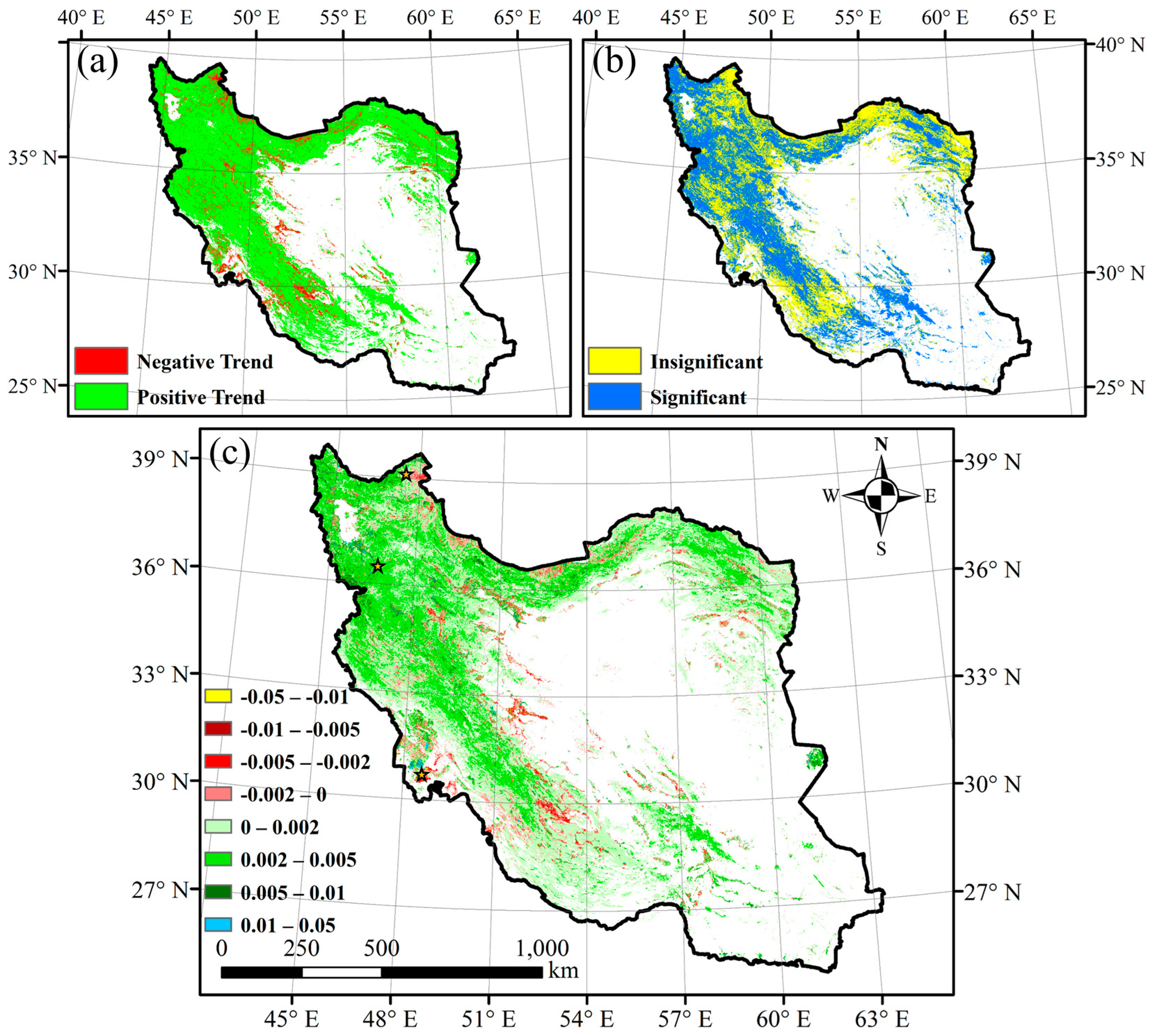
| Slope Magnitude Range | ||||||||
|---|---|---|---|---|---|---|---|---|
| [−0.05–−0.01] | [−0.01–−0.005] | [−0.005–−0.002] | [−0.002–0] | [0–0.002] | [0.002–0.005] | [0.005–0.01] | [0.01–0.05] | |
| Vegetation Pixels | 0.15% | 0.75% | 2.34% | 7.34% | 59.15% | 26.63% | 3.17% | 0.57% |
| Highest Transitions between 2001 and 2020 (Area in km2) | |||||
|---|---|---|---|---|---|
| First | Second | Third | Fourth | Fifth | |
| Linear | B ➔ S (6130) | G ➔ S (5147) | S ➔ G (4651) | B ➔ G (4272) | G ➔ C (3318) |
| Quadratic | B ➔ S (2443) | S ➔ G (1098) | G ➔ S (939) | B ➔ G (779 km2) | G ➔ C (603) |
| Cubic | B ➔ S (7150) | G ➔ S (3821) | B ➔ G (3389) | S ➔ G (2119) | G ➔ C (1474) |
Publisher’s Note: MDPI stays neutral with regard to jurisdictional claims in published maps and institutional affiliations. |
© 2022 by the authors. Licensee MDPI, Basel, Switzerland. This article is an open access article distributed under the terms and conditions of the Creative Commons Attribution (CC BY) license (https://creativecommons.org/licenses/by/4.0/).
Share and Cite
Ghorbanian, A.; Mohammadzadeh, A.; Jamali, S. Linear and Non-Linear Vegetation Trend Analysis throughout Iran Using Two Decades of MODIS NDVI Imagery. Remote Sens. 2022, 14, 3683. https://doi.org/10.3390/rs14153683
Ghorbanian A, Mohammadzadeh A, Jamali S. Linear and Non-Linear Vegetation Trend Analysis throughout Iran Using Two Decades of MODIS NDVI Imagery. Remote Sensing. 2022; 14(15):3683. https://doi.org/10.3390/rs14153683
Chicago/Turabian StyleGhorbanian, Arsalan, Ali Mohammadzadeh, and Sadegh Jamali. 2022. "Linear and Non-Linear Vegetation Trend Analysis throughout Iran Using Two Decades of MODIS NDVI Imagery" Remote Sensing 14, no. 15: 3683. https://doi.org/10.3390/rs14153683
APA StyleGhorbanian, A., Mohammadzadeh, A., & Jamali, S. (2022). Linear and Non-Linear Vegetation Trend Analysis throughout Iran Using Two Decades of MODIS NDVI Imagery. Remote Sensing, 14(15), 3683. https://doi.org/10.3390/rs14153683