Article

Offshore Oil Slick Detection: From Photo-Interpreter to Explainable Multi-Modal Deep Learning Models Using SAR Images and Contextual Data

1
LISTIC Laboratory, Polytech Annecy-Chambery, University of Savoie Mont Blanc, F-74944 Annecy le Vieux, France
2
TotalEnergies S.E., Avenue Larribau, F-64018 Pau, France
*
Author to whom correspondence should be addressed.
Remote Sens. 2022, 14(15), 3565; https://doi.org/10.3390/rs14153565
Submission received: 12 June 2022 / Revised: 13 July 2022 / Accepted: 19 July 2022 / Published: 25 July 2022
(This article belongs to the Special Issue Remote Sensing Applications in Ocean Observation)

Abstract

:
Ocean surface monitoring, emphasizing oil slick detection, has become essential due to its importance for oil exploration and ecosystem risk prevention. Automation is now mandatory since the manual annotation process of oil by photo-interpreters is time-consuming and cannot process the data collected continuously by the available spaceborne sensors. Studies on automatic detection methods mainly focus on Synthetic Aperture Radar (SAR) data exclusively to detect anthropogenic (spills) or natural (seeps) oil slicks, all using limited datasets. The main goal is to maximize the detection of oil slicks of both natures while being robust to other phenomena that generate false alarms, called “lookalikes”. To this end, this paper presents the automation of offshore oil slick detection on an extensive database of real and recent oil slick monitoring scenarios, including both types of slicks. It relies on slick annotations performed by expert photo-interpreters on Sentinel-1 SAR data over four years and three areas worldwide. In addition, contextual data such as wind estimates and infrastructure positions are included in the database as they are relevant data for oil detection. The contributions of this paper are: (i) A comparative study of deep learning approaches using SAR data. A semantic and instance segmentation analysis via FC-DenseNet and Mask R-CNN, respectively. (ii) A proposal for Fuse-FC-DenseNet, an extension of FC-DenseNet that fuses heterogeneous SAR and wind speed data for enhanced oil slick segmentation. (iii) An improved set of evaluation metrics dedicated to the task that considers contextual information. (iv) A visual explanation of deep learning predictions based on the SHapley Additive exPlanation (SHAP) method adapted to semantic segmentation. The proposed approach yields a detection performance of up to 94 % of good detection with a false alarm reduction ranging from 14 % to 34 % compared to mono-modal models. These results provide new solutions to improve the detection of natural and anthropogenic oil slicks by providing tools that allow photo-interpreters to work more efficiently on a wide range of marine surfaces to be monitored worldwide. Such a tool will accelerate the oil slick detection task to keep up with the continuous sensor acquisition. This upstream work will allow us to study its possible integration into an industrial production pipeline. In addition, a prediction explanation is proposed, which can be integrated as a step to identify the appropriate methodology for presenting the predictions to the experts and understanding the obtained predictions and their sensitivity to contextual information. Thus it helps them to optimize their way of working.

1. Introduction

Throughout the era of offshore data, the detection of oil slicks originating from anthropogenic (spills) or natural (seeps) sources has always been a long-standing challenge. Offshore oil slick monitoring is a relevant topic for a broad audience, including scientists, environmentalists, and local authorities. The devastating effects of marine pollution, including the deterioration of aquatic ecosystems, make oil slick detection a mandatory task [1].
Previous studies [2,3] have highlighted the usefulness of Remote Sensing (RS) technology for offshore monitoring. In particular, Synthetic Aperture Radar (SAR) technology has been identified as an effective technology for detecting marine pollution [4,5]. The main advantage of SAR technology is that it is independent of sunlight, weather, and clouds and allows for global coverage. These results provide new solutions to improve the detection of natural and anthropogenic oil slicks by providing tools that allow photo-interpreters to work more efficiently on a wide range of marine surfaces to be monitored worldwide. Such a tool will accelerate the oil slick detection task to keep up with the continuous sensor acquisition. This upstream work will allow us to study its possible integration into an industrial production pipeline. Nevertheless, slick detection has remained a challenge due to the high variability of their nature, shape, and extent. Oil slicks have no typical characteristics and vary according to the environment and surrounding conditions, which makes their detection very complex. As oil slicks are present on the sea surface, their shape depends on weather conditions and their source (e.g., an elongated dark patch if the origin is a moving ship or a random pattern if it comes from a platform or natural seepage). In addition, the acquisition time of the SAR image containing the oil is delayed relative to the time of its appearance. Thus, the shape of the oil slick then has time to evolve significantly with the help of weather conditions that influence the physio-chemical properties of the oil slick (e.g., fragmentation of the slick into droplets, dissolution in seawater, etc.). Another challenge is the potential confusion with similar patterns such as algae, low wind areas, and up-welling [2].
Indeed, multiple studies such as Brekke et al. [4], Alpers et al. [2], Solberg et al. [6], and Espedal [7] point out that improving slick detection using SAR requires the inclusion of more ancillary contextual information such as meteorological information. Finally, from an application point of view, an additional challenge relates to the fast processing of large quantities of data to assist human experts in real-time monitoring. Such an aim is actually no more feasible by sole human experts when considering the high spatial resolution and high revisit frequency of the sensors required for the task.
The state-of-the-art on this topic involves manual inspection, pattern detection, and thresholding methods based on various feature categories [8,9]. However, the latter exhibit poor generalization behavior and lack robustness against false detection due to lookalikes.
Neural networks and, more particularly, deep neural networks (DNNs) [10] have recently shown an increasing interest in improving over classical approaches both in terms of detection accuracy and generalization capability [11]. However, those works rely on the sole use of SAR images.
In this paper, we study offshore oil slick detection using deep neural network approaches in a supervised manner, taking full advantage of massive annotated datasets of real recent slicks monitoring scenarios manually annotated by human experts (photo-interpreter). The objective is to provide new solutions to improve the detection of natural and anthropogenic oil slicks by providing tools that allow photo-interpreters to work more efficiently on a wide range of marine surfaces to be monitored worldwide. This tool will speed up their detection task to keep up with continuous sensor acquisition. As this is a difficult task with many challenges, including high target variability and the potential for false alarms, providing rapid predictions should be valuable.
To this end, we consider multi-modal deep learning approaches, allowing heterogeneous data fusion taking into account SAR images and wind information.
To the best of our knowledge, this is the first study combining meteorological information with SAR data and evaluating the impact of wind speed on slick detection on a broad collection of data spanning different regions in the world with a wide diversity of real slick cases. This upstream work will allow us to study its possible integration into an industrial production pipeline.
This paper presents the following contributions: first, a slick detection performance analysis of structurally different deep neural networks is conducted. Second, a new deep neural network model structure considers the fusion of SAR information with wind speed information. Third, a refined performance analysis method is proposed, taking into account contextual factors such as wind speed and human infrastructure position. Finally, model prediction explanations are proposed. It relies on adapting the SHAP [12] method to the semantic segmentation problem and allows the input features contributing to the local decision to be highlighted.

1.1. Offshore Oil Slick Detection and the Related Literature

1.1.1. Oil Slick Observation on the Sea Surface

Oil slicks observed on the sea surface are commonly of two types: spills and seeps. The causes of oil spills can be discharges of crude oil from tankers, offshore platforms, ships, drilling rigs, and spills of refined petroleum products or used oil. On the other hand, seeps are naturally occurring oil flows that escape from the ground through soil fractures and sediments to the sea surface.
These differences in nature lead to variations in oil slick characteristics, such as viscosity and thickness, resulting in different behaviors and increasing the variability of oil slick observations.
The observation of offshore oil slicks is conducted mainly by RS, specifically by active sensors such as SAR. SAR technology relies on ElectroMagnetic (EM) signals sensitive to the sea surface roughness. The intensity of SAR images is related to the strength of the backscattered radar signal. In more detail, the energy transmitted by the SAR sensor is backscattered with characteristics that highlight the properties of the areas involved. In the case of a calm sea, most of the transmitted energy is reflected away from the radar, resulting in minimal backscatter to the sensor and a darker area on the resulting image. Conversely, in the case of a rough surface due to wind, a more significant part of the EM energy is backscattered from the surface [2] and thus yields a brighter area with speckle noise.
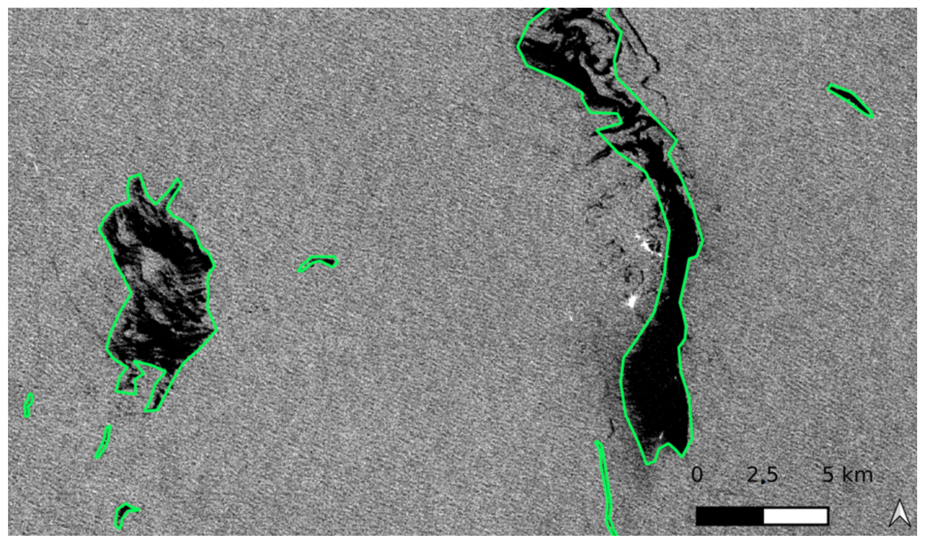
Further, if an oil slick appears, it dampens the waves on the sea surface, reducing the surface roughness and the corresponding radar backscatter. This is due to the viscous damping of short gravity/capillary waves (wavelengths of a few centimeters) by the oil slick or oil/water mixture, whose viscosity is much higher than water [2]. As a result, oil slicks appear on SAR images as dark patches compared to the surrounding clean sea, as illustrated in Figure 1. Slick characteristics are widely variable, such as the contrast value, which depends on the local sea state, the slick type, the image resolution, the SAR frequency, and the incidence angle.
Besides the oil slicks on the sea surface, several phenomena referred to as lookalikes can generate similar radar signatures (low backscatter areas) that can yield false alarms (FA). This generally originates from algal blooms, sargassum, and upwelling [4]. More generally, any patch that is darker than the surrounding area could be an oil slick. Illustrations of spills, seeps, and lookalikes are shown in Figure 2.
To summarize, the main factors involved in oil slick detection from SAR images are related to contextual information such as wind conditions, sensor characteristics, and the presence of lookalikes.

1.1.2. Contextual Data: Impact on Oil Slick Detection

In oil slick detection, numerous studies have emphasized the importance of contextual information as the main factor impacting the monitoring of offshore oil slicks using SAR imagery. The study proposed by Brekke et al. [4] highlights the interest in weather conditions, distance from ships, and infrastructure position (platform, pipeline, etc.). Meteorological weather conditions are emphasized, namely wind speed, which affects the oil slick profile (oxidation, biodegradation, dispersion, sedimentation, etc.) and changes its characteristics (size, shape, etc.) [14]. In addition, wind speed impacts the backscatter contrast between the sea and slick areas. On the one hand, oil slicks tend to scatter gradually into smaller parts at moderate wind speeds and disappear as wind speed increases. On the other hand, local low wind speeds can generate areas of low backscatter and, therefore, lookalikes [15]. Observing the effect of wind on slick characterization reveals the apparent importance of this information in the slick detection and characterization process.
Moreover, during oil slick manual detection by the photo-interpreters, the evaluation can be adjusted by taking the instantaneous wind speed into account. According to Fingas et al. [3], the wind speed range for oil detectability is (1.5 m/s, 6–10 m/s). Beyond this range, the oil signature will be further removed. The most accepted limits are 1.5 to 10 m/s. La et al. [16] and Brekke et al. [4] have further refined this range, a summary of which is provided in Table 1. However, it may remain specific to small-scale, local studies that do not permit generalization. As a general rule, these experiments report the requirement for moderate wind speeds. This paper considers a trade-off between the proposed wind speed ranges that seems relevant to our large-scale study.
Further, in the process of oil spill detection, the photo-interpreters are informed about the positions of the infrastructure since pollution can originate from human activities. The deballasting of the ship hold is easily recognizable thanks to the strong backscattering point created by the ship at the end of the oil slick when the SAR image is captured. The geometry of the oil slick is also generally straight along the ship’s path due to the speed effect. Oil spills can also originate from underwater infrastructures and conduits (pipes) designed to carry oil. For the situations mentioned above, ship and platform positions can be spatially detected based on the diffraction points observed in the SAR images. This can help distinguish anthropogenic oil from natural oil based on the distance of the slicks from the infrastructure in the area [2].

1.1.3. Classical Methods for Oil Slick Detection

The state-of-the-art of offshore oil slick monitoring is extensive. A brief classification of the main approaches is presented below based on the surveys proposed by Alpers et al. [2], Brekke et al. [4], and Al-Ruzouq et al. [18].
Entirely Manual Inspection: Oil slick detection on SAR images is essentially manual. Operators (photo-interpreters) are trained to analyze images to detect oil slicks versus lookalikes and differentiate between natural and anthropogenic oil. The class assignment (spill, seep, sea including lookalikes) is based on the following features: the contrast level with the surroundings, the homogeneity of the surroundings, the wind speed, the oil platforms, ships and natural slicks in the proximity, as well as the shape and edge of the patch. This detection method is tedious, time-consuming, and costly regarding resources.
Conventional Approaches: This category of approaches focuses mainly on three steps: the first is to detect the dark patterns, the second is to extract their features, and the third is to classify them [3]. Conventional features can belong to several categories, such as geometric, statistical, and polarimetric features [4,19,20]. Such approaches, however, exhibit poor generalization behavior and lack robustness against lookalikes [18,21].
Semi-Automatic Approaches: Some processing stages of the conventional approaches, such as dark pattern detection, can rely on machine learning. For instance, the integration of Neural Networks improves the traditional process. Nevertheless, such a general approach still has limited generalization behaviors and keeps high false alarm rates [2].

1.1.4. Deep Learning Methods for Oil Slick Detection

Various facts have directed the search for the automation of oil detection toward end-to-end approaches driven by deep Convolutional Neural Networks (CNNs). Among these is overcoming the shortcomings of conventional approaches reported by state-of-the-art; lack of studies on both oil types, lack of relevant features to distinguish oil slicks from lookalike phenomena and the limited generalization capability. The remarkable results of CNN-based approaches have led to dramatic advances in the state-of-the-art for fundamental computer vision problems such as object detection, object localization, and semantic and instance segmentation [22,23,24]. Several studies have compared deep learning techniques to classical classifiers and indicated better performance with deep learning techniques [20,25]. The studies report the ability of CNNs to perform both feature extraction and classification, allowing the exploration of relevant features for better discrimination between the oil slick and background patterns. The ability of the CNN network to leverage the extensive existing data can ensure a certain level of generalization capability [18].
Table 2 reports examples of recent NN models applied to oil slick detection and segmentation from Sentinel-1 images, indicating the type of oil spill targeted by the study along with the number and size of the used images. Various models of NNs are proposed; some perform semantic segmentation, such as Unet [26], and others perform object detection and instance segmentation, such as Mask R-CNN. It should be noted that few annotated SAR data are available, which limits supervised learning of large models and explains the use of Transfer Learning (TL) strategies, i.e., representations of data preliminary learned in other tasks and domains.

2. Materials and Methods

2.1. Oil Slicks Segmentation Methods

In this study, we consider both transfer learning and full model learning (learning from scratch). For the first method, the model is pre-trained on a different dataset and task and is next transferred and fine-tuned for oil slick detection on dedicated datasets. As for the second method, we focus on model optimization exclusively performed on the data of interest without any pre-training.
Since the goal is to find the precise location of oil slicks in SAR images, standard object detection methods are not appropriate because they commonly provide object bounding boxes that may be too large compared to the thin oil slicks to be detected. In this case, the segmentation of oil slick instances is more relevant. Such a strategy opens wide doors to a variety of approaches. In this work, a comparison is made between a convolutional neural network, for instance, segmentation: Mask Region-Based Convolutional Neural Networks (Mask R-CNN [32]) with object segmentation capability and a semantic segmentation neural network Fully Convolutional DenseNet (FC-DenseNet [33]). Instance and semantic segmentation methods are comparable in this case study since we do not face occlusion issues of oil slicks on the sea surface. Consequently, applying connected components to the semantic segmentation predictions yields instance segmentation.
As for our experimental strategy, we first compare the performance of models using only SAR data in order to identify the best parameter configuration (number of layers, learning rate, etc.). Then, we investigate heterogeneous data fusion strategies to fuse wind speed information with SAR information.

2.1.1. Instance Segmentation: Mask R-CNN

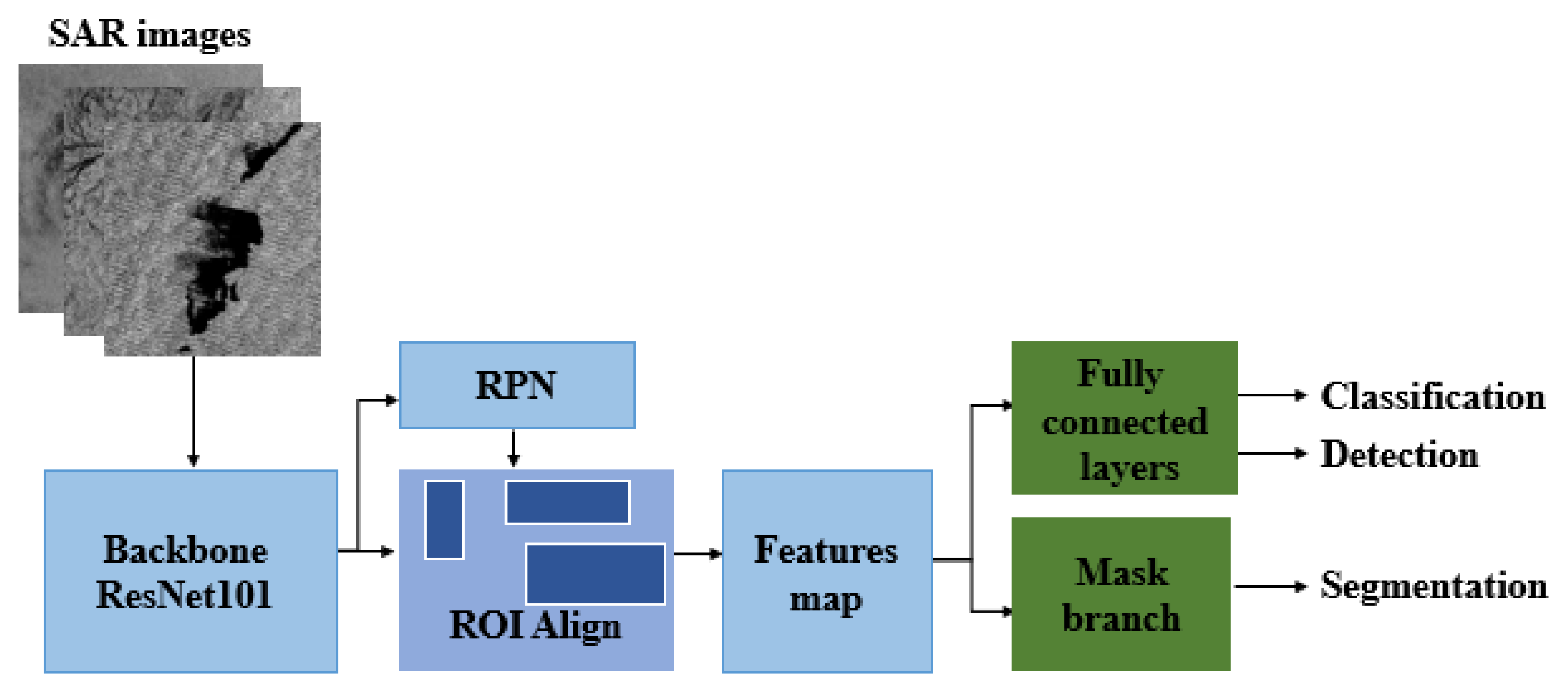
Mask R-CNN is a multi-task model that generates bounding boxes of the target object regions, as well as masks for object classification and segmentation. The first step is to extract features r from the input x using the parameter set θ b , such that f b ( x , θ b ) = r . Then, the features are passed to several heads f t i ( r , θ t i ) = y t i , with t i referring to the i t h task.
The model is shown in Figure 3. Nevertheless, this complex deep architecture must be trained by transfer learning when targets are scarce. As described in a previous study [28], the parameters of a pre-trained model are transferred from the COCO dataset [34]. Subsequently, we gradually adjust the transferred weights on our data, starting with the heads and moving towards the backbone. This whole process is achieved while reducing the learning rate as described in the following.

2.1.2. Model Parameters Configuration

The implementation from Abdulla [35] was adopted to accommodate the Mask R-CNN model. Several experiments were performed to select the parameters and adapt the problem properly; the main ones are described below.
Backbone selection: The backbone network could be any CNN designed for image classification, such as ResNet-50 or ResNet-101.
Loss selection: Since oil slicks are scarce and diverse, one needs to down-weight easy examples and focus the training on hard ones. Thus, we use the focal loss [36] instead of the cross-entropy (CE) for mask loss computation. This loss is also more adapted than CE for highly imbalanced classes. It is formulated as follows: L ( p t ) = α t ( 1 p t ) λ l o g ( p t ) where p t is the model’s slick detection probability. The role of the α t and λ parameters is to down-weight easy examples (error loss) and thus focus training on hard negatives [36].
Learning strategies: as reported in [28], relevant optimization of Mask R-CNN can be achieved with multiple training phases. This decomposition can give us training flexibility. The primary approach is to train all the networks in a single stage. A second approach consists of two steps: training the model heads first while using transferred weights for the rest of the network, then fine-tuning all networks. Finally, the three-step learning strategy trains the model heads over a few epochs first while also using transferred weights. Then, all but the first four ResNet layers are trained over additional epochs. Finally, the entire network is fine-tuned while reducing the learning rate. For this work, the approach used is to train the model based on the three-step learning strategy.

2.1.3. Semantic Segmentation: FC-DenseNet

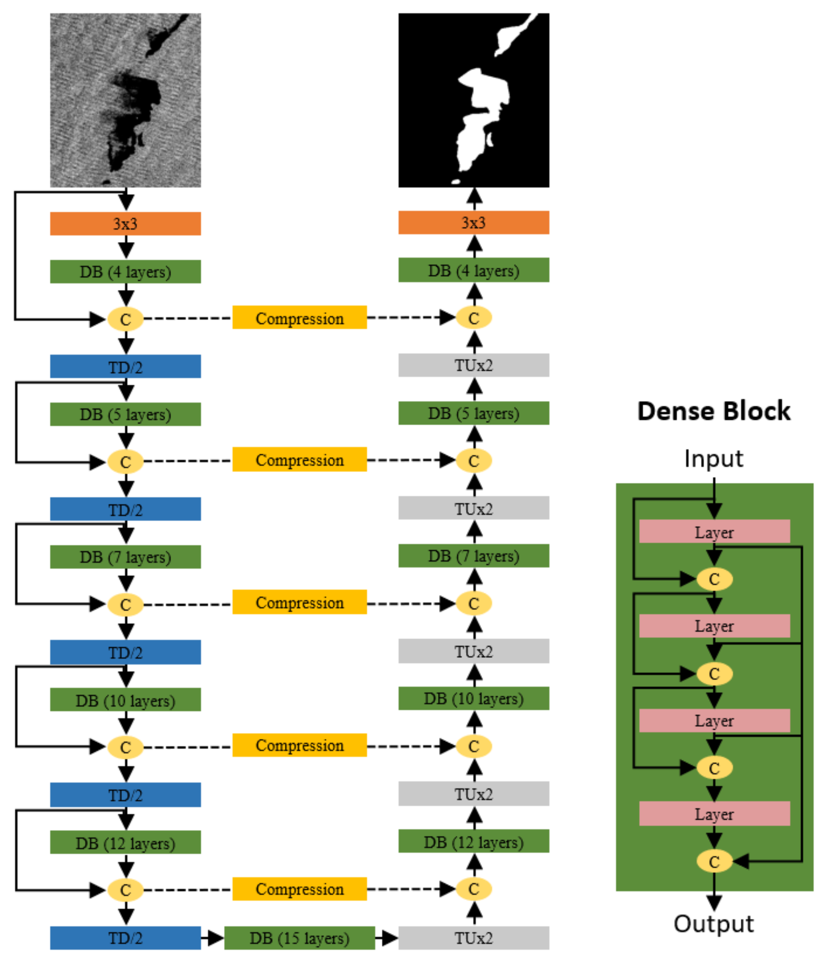
We propose a refined version of the FC-DenseNet model [33], a well-known extension of densely connected convolutional networks (DenseNets) [37]. The DenseNets architecture has been proposed to maximize feature reuse and limit the model depth and computational costs compared to the classical U-net structure [38]. The FC-DenseNet extends the DenseNets classification architecture to perform semantic segmentation by adding an upsampling path to perform pixel-level classification. This architecture belongs to the category of encoder-decoders, as shown in Figure 4. It is built from dense blocks and sampling operations.
This architecture uses the so-called skip connections, allowing the transmission of low-level feature maps from the encoder to the decoder. The decoder thus performs a concatenation of the low-level abstract feature provided by the encoder with the high-level semantic feature available in the decoder. This results in a more refined and more accurate prediction map that fully exploits the details of the high-resolution first model features. Moreover, skip connections facilitate the model learning by transmitting the gradient error directly to the first layers of the model and thus reducing gradient fading. Similarly, at the dense block level, skip connections are used. All previous layer feature maps are concatenated and used as inputs for each layer, and their feature maps are used as inputs for all subsequent layers. Each layer generates an activation map designed according to a connectivity pattern that iteratively concatenates all feature outputs in a feed-forward approach, according to Equation (1) [33]:
f l = H l ( { f l 1 , f l 2 , , f 0 } , θ l )
where f l indicates the output feature map of the lth layer. It is computed by applying a non-linear transformation H l on the concatenation of the previous layers’ feature maps f l 1 , f l 2 , , f 0 . H l is a non-linear transformation defined as a convolution with trained parameters θ l , followed by a R e L U and dropout. It then maximizes feature reuse and facilitates the training of deep structures.

2.1.4. Model Parameters Configuration

Intensive experiments were conducted to search for the best model and to select the appropriate parameters. The main ones are described below.
  • Optimizer: Different gradient-based optimization algorithms of objective functions have been introduced so far, such as Stochastic Gradient Descent (SGD) [39], Adam [40], and RMSprop [40]. Driven by the work of Kingma et al. [40], we use the Adam algorithm in our work. It is computationally efficient, requires little memory, is invariant to the diagonal scaling of gradients, and is well suited to large problems in terms of data and/or parameters. We consider an initial learning rate of 0.00005 to begin the learning. Subsequently, a learning rate decay policy is applied: it is reduced by a factor of ten if the validation loss has not improved in the last 150 epochs. This latency time does not result in an over-fitting, thanks to the dropout existing in all the model layers.
  • Loss function: An extreme imbalance is observed between foreground (slicks) and background (sea) classes on the considered data collections. A set of losses has been experimented with, such as focal loss [36], dice loss [41], and cross-entropy. The main objective is to select a loss taking into account the class imbalance, focusing the training on difficult cases. The loss chosen based on the experiment is the sum of the dice loss and the cross-entropy.
  • Batch size: Batch size, rather than optimizing the network from one sample at a time, leading to non-optimal solutions, averaging the errors over a set of samples has proven to be more efficient. We use a batch of 4 samples due to hardware limitations.
  • Model depth and width: We experiment FC-DenseNet with various hyper-parameter combinations controlling model depth (number of dense blocks) and width (number of neurons per layer, also referred to as growth rate). Experiments show that a higher depth gives the best results. We chose to set the number of dense blocks to 5 and the number of feature maps per layer to 16. Thus, the total number of parameters of the corresponding model is about 8 M.

2.1.5. FC-DenseNet Model Enhancements

We propose an improved version of the FC-DenseNet model based on several optimizations listed below.
  • Layer initialization: The choice of initial parameter values for gradient-based optimization is very crucial. Following [42], we chose random orthogonal initial weights to start with complementary operators and to accelerate the convergence compared to a Gaussian initialization. Such an approach indeed leads to faithful gradient propagation, even in deep non-linear networks, by combating exploding and vanishing gradients. Further, regarding the initialization of the last linear classification layer, it is common to use a bias b = 0. However, Lin et al. [36] point out that this could cause instability during training for obtaining class probabilities. Therefore, for training, we initialize the bias of the last layer as b = l o g ( ( 1 c f ) / c f ) , where c f = 1 / C where C is the number of classes.
  • Non-linearity: In the original FC-DenseNet model, R e L U ( x ) = m a x ( 0 , x ) is considered as an activation function. Its main advantage is the non-saturation of its gradient, which leads to faster convergence of the training process [43]. Improved versions of ReLU activation have been proposed, such as Leaky-ReLU [44]. Such activation enables the transformation of the negative input signal instead of canceling it as for ReLU. This activation can interest classical model structures with no or few skip connections to avoid losing important information. However, the dense blocks of the model allow all the data to be shared across layers with dense connections, thus maximizing feature reuse before applying activation functions and justifying the use of RELU.
  • Model regularization: Original FC-DenseNet relies on batch normalization with large batch size. However, small batch size is required to handle large images while working with limited GPU memory. In this situation, batch normalization is discarded. A chosen alternative is the use of Spectrum Restricted Isometry (SRIP) weights regularization [45] for all but the last layer. This regularization technique does not induce additional computation at test time and provides notable advantages: it ensures feature normalization while maintaining the orthogonality of neuron parameters throughout the training, which is complementary to the initialization strategy [45]. This approach then ensures that neural kernels act in a complementary way, which is relevant when dealing with few feature maps per layer as for the FC-DenseNet structure.
  • Skip connection compression: It aims at reducing the size of the features passed from the encoding part to the decoding one. Actually, for the vanilla FC-DenseNet, the dimensions of the low-level features outing from the encoder to be fused with the decoder features are higher than their counterpart. A compression then allows for a balance of feature dimensions and reduces model complexity on the decoder side. In this work, compression consists of 1 × 1 convolutions. The compression ratio is adjusted so that the feature maps of the skip connections and the previous dense block have the same size before they are concatenated.
  • Upsampling: Transposed convolutions are generally considered but tend to introduce checkerboard artifacts on the outputs [46]. An alternative is to separate upsampling to a higher resolution from convolutions to compute features. We then first resize the image using nearest-neighbor interpolation and then apply 2D convolution layers as proposed in [47].

2.1.6. Detecting from Heterogeneous Sources, Fuse-FC-DenseNet

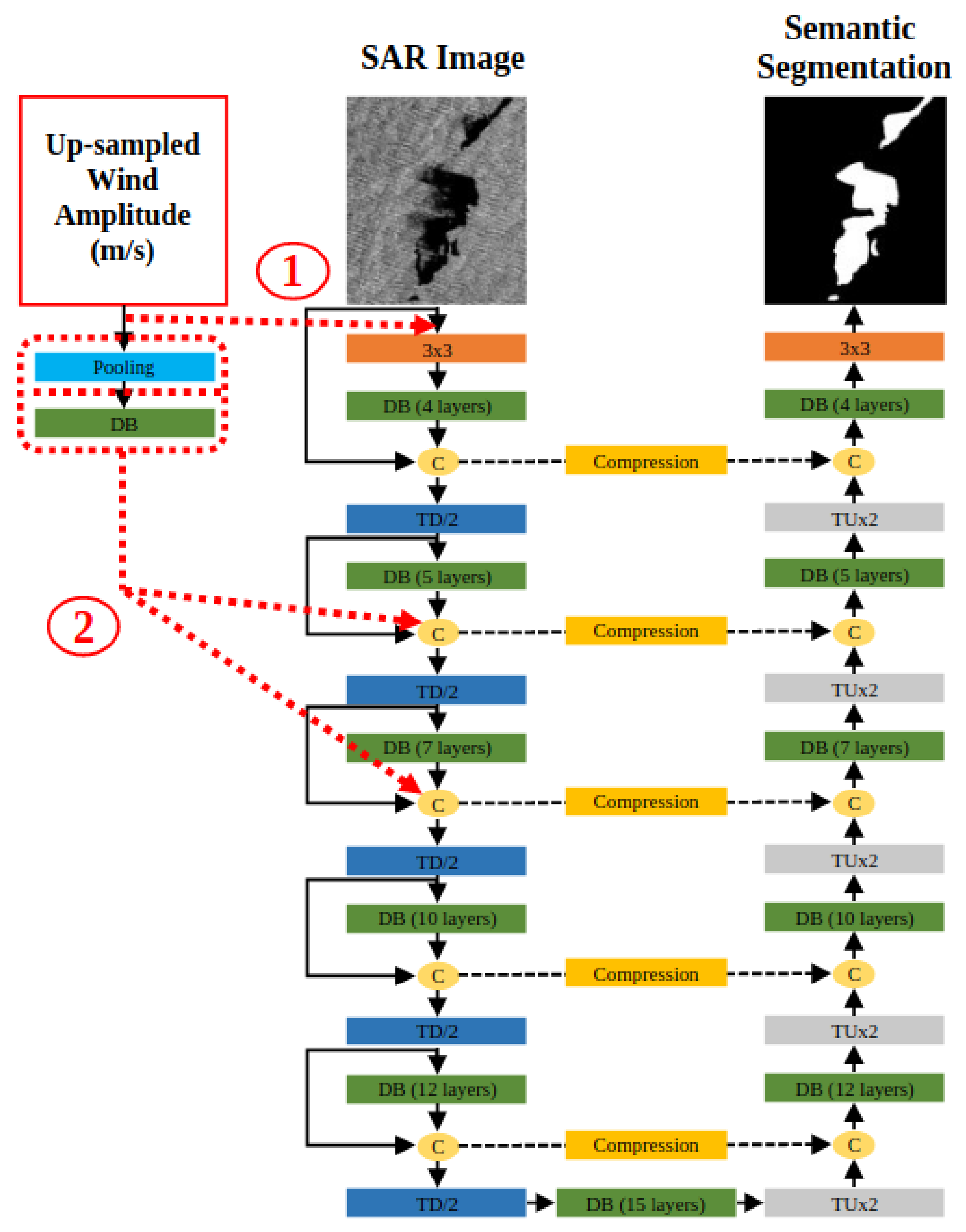
Since the radar backscatter at the sea surface is deeply affected by the wind speed, as detailed in Section 1.1.2, the fusion of wind speed with SAR information is an exciting approach for oil detection. In this work, the fusion of wind and SAR data is performed in two different ways, as illustrated in Figure 5 (1 and 2).
(1)
Early fusion: Wind and SAR modalities are considered at the same level. Thus, the network input consists of the SAR data channel and the corresponding wind speed channel, resampled during the data processing step to match the SAR image resolution.
(2)
Late fusion: The SAR and wind modalities are considered as two specific input channels with their separate layers before their fusion. In this approach, while keeping the enhanced FC-DenseNet structure for the SAR data, the wind modality is introduced in subsequent dense blocks along the model encoding path. The merging process is performed after the second or third block so that the wind features at their original scale are fused with the SAR features when the latter reach a similar resolution after a few downscaling steps along the encoding section. As for the general DenseNet approach, this fusion operation consists of concatenating the features of each channel. Regarding the processing of wind channels, several strategies can be investigated. In this paper, we consider two approaches: (i) applying a simple average pooling to adjust feature scales and (ii) applying mean clustering and then extracting higher-level features with a dense block.

2.2. Experimental Data

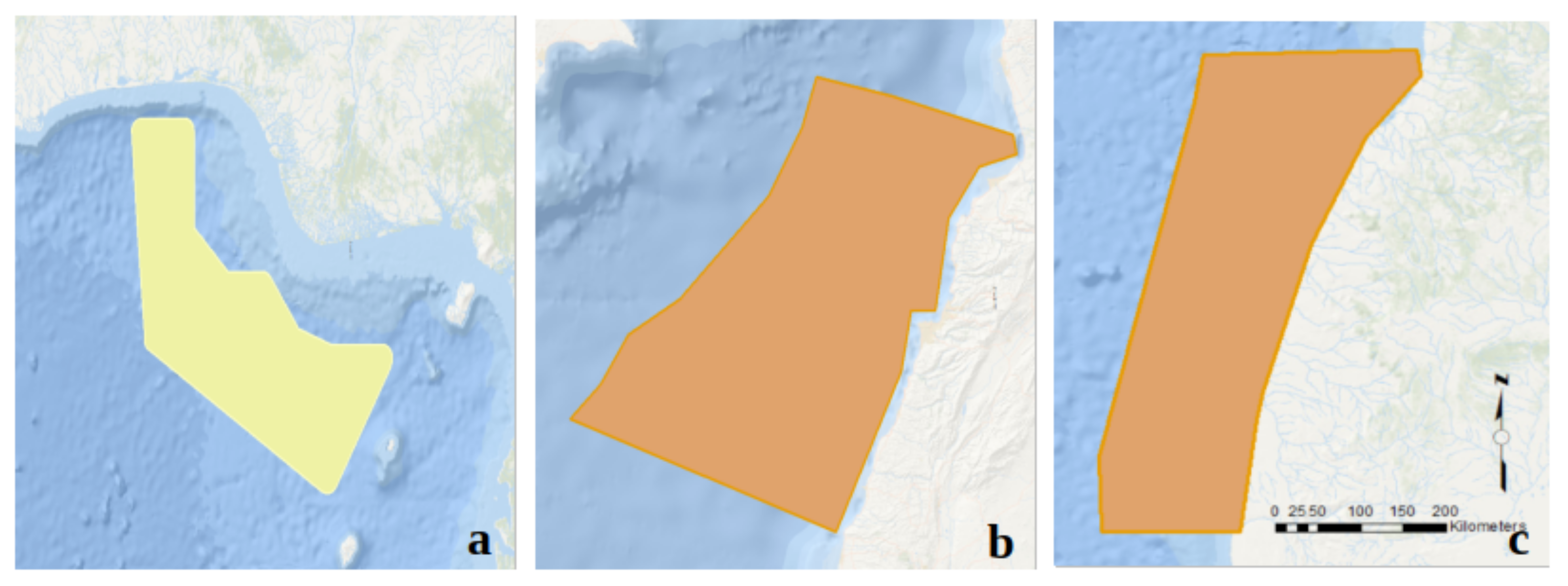
The experimental data considered in this work are acquired over four years (2015–2019) in three separate study areas shown in Figure 6. The training, validation, and test datasets were acquired in these three areas but differed in acquisition date and coverage. This location diversity enriches our database with a larger area to explore and more variety in terms of statistics (weather, infrastructure, etc.). Below is a description of all the data considered in our study.
  • Sentinel-1 SAR data: Acquired by the European Space Agency (ESA) organization in Interferometric Wide-swath Mode, C-band (5.40 GHz) and with a 10 m resolution per pixel. The level of signal backscattered by the sea surface is higher for vertically polarized waves (V) than for horizontally polarized waves (H) [48]. Hence, vertical polarizations for transmission and reception (VV channel) are selected as they are generally preferred to the HH channel for ocean studies [49]. A set of 1428 images is considered in this study.
  • Slick annotation (Ground Truth): Human experts performed manual annotation of natural and anthropogenic oil slicks. The considered classes are: sea, spill, and seep. Importantly, this study is based on real-world monitoring scenarios. Under these conditions, the photo-interpreters cannot provide accurate annotations on object boundaries due to the fuzzy contours of the slicks and the annotation rhythm. Therefore, the annotations show sharp transitions that do not reflect the actual slick shape. Further, slick annotation is performed by five photo-interpreters, revealing a diversity of annotation criteria. For example, some slick annotations do not match the black slick perfectly and are shifted by a few pixels. Others account for small slick patches separated from the main slick and displaced. The difference is shown in Figure 2a–j. Figure 7 shows an example of image annotation. One can then consider that annotation is noisy but satisfies operational monitoring requirements.
  • Wind speed information: Wind speed estimates for each SAR image are also provided. The estimation is performed based on empirical Geophysical Model Functions (GMFs), relying on the relationship between the backscatter and the wind speed. For C-band and VV polarization, several variants of GMFs named CMODs have been developed [50]. The CMOD5 variant is a version that has been used successfully as an improvement of the above variants. It is formulated as Equation (2):
    σ C M O D 5 0 ( V , ϕ , θ ) = b 0 ( 1 + b 1 cos ϕ + b 2 cos ϕ ) 1.6
    where the variables are:
    • σ C M O D 5 0 : backscatter value of the model CMOD5,
    • V: wind speed (m/s),
    • ϕ : relative direction between the radar look direction and the wind direction,
    • θ : angle of incidence,
    • b 0 , b 1 , b 2 : functions of wind speed V and incidence angle θ .
    CMOD5 estimates the radar backscatter in a scene as a function of the surface wind speed (V) and the angle that the wind makes with respect to the direction of the pulse ( ϕ ) and the incidence angle ( θ ) [51]. However, for surfaces such as slick areas, the wind speed is underestimated due to the wave damping effect. This discrepancy has been considered at the model performance assessment step.
    In our context, SAR and wind resolutions are 10 and 100 m per pixel, respectively, such that wind is upsampled by a factor of 10 using linear interpolation when required. An example of a Sentinel-1 SAR image before and after adaptation to CMOD5 is shown in Figure 8.
  • Infrastructure Position: This information is known using global referencing, which represents support for photo-interpreter analysis [4]. Through the use of infrastructure position, we further improve the evaluation of model performance in terms of detecting anthropogenic oil. The types of infrastructure considered are pipelines, wells, ports, platforms and ships. For each of them, there is a possibility of leakage accorded to the experts. The location of the infrastructures is associated with the SAR images, as shown in Figure 9.
To summarize, for each SAR image available in the dataset, the associated wind speed, infrastructure position and slick annotation are provided.

2.2.1. Data Preprocessing

To enable heterogeneous data processing, we describe below the preprocessing of each data and its purpose.
  • SAR Data: The preprocessing of initial SAR data consists of low-level transformations to improve the qualitative and quantitative interpretation of image components, thus facilitating the visibility of slicks for photo-interpreters. SAR preprocessing can be grouped into four processes: radiometric calibration, geo-referencing, filtering, and masking [18].
    (1)
    First, radiometric correction and calibration: Its purpose is to remove or minimize radiometric distortions and to ensure the correlation of pixel values with the backscatter coefficient of the reflecting surface [52]. Thus, quantitative measurements (backscattered microwave energy) restored from image pixel values can be compared with object characteristics in multi-temporal SAR images acquired with different sensors and SAR modes [53].
    (2)
    A geo-referencing step of the SAR data is then performed to correct eventual geometric distortions and to locate each pixel of the image on the Earth [54]. This step is also applied to all the considered data sources to ensure their alignment.
    (3)
    A speckle noise filtering step is then performed. As reported by [3,55], such noise must be reduced in order to facilitate the analysis and interpretation of the data. An optimal speckle filtering technique should preserve useful radiometric information and avoid the loss of features, such as the local mean of backscatter, texture, edges, and point targets [56]. Several filter types have been used in previous studies to reduce speckles and enhance SAR images for oil slicks, such as Lee, Frost, Kuan, median, and Lopez [57]. The considered preprocessing pipeline relies on such filters, but its detailed implementation remains confidential.
    (4)
    The final preprocessing step consists of masking the land and shorelines from the SAR images. This process restricts sea surface analysis and prevents land from interfering with oil slick detection [58].
  • Wind data: For each 10 m resolution SAR image, the associated wind intensity map is provided with the same geographic coverage but at 100 m resolution. Therefore, to align the two modalities, bi-linear interpolation is applied to the wind map. However, the wind speed is underestimated over the slick areas due to the wave damping effect. Then, specifically for the test set and evaluation process but not for the training set, the wind speed, in the vicinity of 50 m around the annotated slicks, is merged within the slick area, relying on iterative median filtering.
  • Infrastructure data: It is based on the infrastructure position; a map that represents the proximity of existing infrastructure in the neighborhood for each pixel is realized. These distance maps will be considered only in the evaluation process.

2.2.2. Preparation of the Training/Validation Datasets

After processing the different data modalities separately, an alignment of each SAR image with the corresponding slick annotations, wind speed map, and infrastructure distance map is performed. Then, datasets of heterogeneous data are built for training, validation, and testing sets. The strategy is described below.
(1)
Dataset Splitting: Following our previous study [28], both training and validation sets rely on the same geographical areas. However, they do not share the same images; each has a different capture date and sea coverage. A third area (Nigeria) is chosen for testing to validate the generalization capability of the model.
(2)
Image Crop Selection: We built a collection of smaller image crops of 512 × 512 pixels from the large images of the training and validation datasets. This resolution is a compromise between the size of the layer, the field of view of the model, and the memory constraints of the GPUs (NVidia V100 16 Gb).
The crop selection strategy takes into account the slick annotations and ensures the presence of slicks within crops following the logical function presented in Equation (3):
C s l i c k ( X , Y ) = ¬ B ( X ) ( E ( Y ) > T )
where ∧ and ¬ are the logical AND and NOT operators, respectively, X is a random crop in a large SAR image, Y is the corresponding annotation, B ( X ) a Boolean function that checks if there is a border (no data area) inside the crop, E ( Y ) is the entropy function used to check the sea and slick classes statistics within the crop, and T is a threshold fixed heuristically to 0.3 .
Further, to make the model robust against slick lookalikes, an additional crop selection of such potential patterns is built from the slick-free image areas. Since no specific annotation reports them, we rely on a heuristic reported in Equation (4), the objective of which is to choose crops with contrasting patterns:
C l o o k a l i k e s ( X ) = ¬ B ( X ) V ( X ) ¬ E ( Y ) ) )
where ∧ is the logical OR operator, B ( X ) and E ( Y ) correspond to the ones described in Equation (3), and V ( X ) is a Boolean function that randomly selects the crop that probably contains lookalikes based on the normalized variance of the pixel values. A minimal variance threshold fixed on the basis of experiments must be reached to highlight a contrasted area.
(3)
Data Augmentation: It is applied to increase the variability in the dataset artificially. It is comprised of random horizontal and vertical flipping and ±90 random rotation in both training and validation datasets [59].
Table 3 outlines the details of the training and validation datasets. A total of 85% of the crops in the dataset belong to the training set. We notice that the oil slicks are small to medium in size compared to the large sea area, covering less than 11% of the total area. This emphasizes the strong imbalance in the number of slicks pixels and the clean sea pixels that include lookalikes.

2.2.3. Test Dataset

Many images are captured in an additional region close to Africa that has not been used for training/validation. This region provides the opportunity to test the generalization ability of our models through a variety of meteorological conditions. Table 4 indicates the characteristics of the test set. It contains 214 oil slicks that give a broad representation of the shape and variation in slick type (spill, seep). One must highlight that this diversity is originally compared to state-of-the-art, which is mainly limited to a single type of oil slicks. This data collection also contains several lookalikes phenomena, such as windless areas. The cost of preparing this data limits the number of samples available, but it represents relevant real-world monitoring and annotation scenarios.
Figure 10 shows the distribution of oil slick annotations as a function of wind speed, slick size, and proximity to infrastructure. Regarding wind speed, most slicks have been annotated at medium wind speeds (3 m/s), few were annotated at very low wind speeds, and none at wind speeds above 6 m/s. As for the size of the slicks, it varies from a few hm2 to 10.000 hm2. The proximity to infrastructure ranges from being very close to being 70 km away from one. This figure illustrates the diversity of the targets and the strong imbalance of their behaviors, which explains the difficulty of their detection.

2.3. Performance Assessments

A set of metrics adapted to the task and operational context is selected. The first category corresponds to standard measures considered for semantic segmentation and object detection. These metrics are reported by taking into account contextual information such as the size of the slick, the local wind speed, and the position of infrastructures. We also rely on ROC curves to visualize the trade-off between detector hit (true positive) rates and false alarm (false positive) rates. The second category of metrics relies on a visual explanation of the model predictions.

2.3.1. Standard Metrics

Semantic Segmentation Quality Metric (pixel-level): A pixel-level classification metric such as the Intersection over Union (IoU) is the most used metric to evaluate models in image segmentation tasks [60]. However, its relevance is moderate in our case since the annotation is noisy.
Standard Object Detection Metrics (instance level): Such metrics describe the detection potential of the model better rather than the segmentation quality. Detection rates and the associated false positives and negative rates are thus computed. Further, in the proposed context, the fragmentation of a single slick in multiple detection instances is not an issue. Therefore, if more than one prediction intersects the same annotated slick, detection is considered valid for this slick. The number of well-detected instances is calculated according to Equation (5).
D e t e c t e d I n s t a n c e s = i = 1 N G t i P r e d
where N is the number of annotated slick instances, P r e d is the predicted instances, and is the indicator function.
Receiver Operating Characteristic curves (ROC): These curves are used to characterize a model segmentation quality in a more detailed way. Such ROC curves are obtained by plotting the True Positive Rate (TPR) as a function of the False Positive Rate (FPR), thus quantifying the performance of a detector as its discrimination threshold varies. In other words, ROC curves describe the trade-off between detector hit rates and false alarm rates [61].

2.3.2. Prediction Explanation Methods

Several model explainability techniques have been proposed to facilitate the understanding of complex model predictions. The best known, according to the study of Linardatos et al. [62], are listed below.
  • Class Activation Maps (CAM)-based methods, e.g., Grad-CAM [63,64], are designed to generate heat maps of the input, indicating which areas most influence the network decision. It relies on a linear combination of activation maps of a given layer, weighted with the gradient of the class score, with regard to the feature map activation. CAM-based methods have some drawbacks: first, explanation precision is limited given that the produced heatmap is computed based on low-resolution activation maps and further upsampled to match the original image size. Second, it does not provide information on negative contributions (inhibition effects).
  • Local Interpretable Model-agnostic Explanations (LIME) [65] is a model-agnostic method that aims to locally (e.g., for one set of inputs) approximate the complex model to a more easily understandable one. This method aims to produce visual artifacts that provide a good understanding of the model choice. However, the LIME method can be criticized for its lack of stability and the discrepancy of its results with human intuition.
  • Layer-wise Relevance Propagation (LRP) [66] uses calculation rules to backpropagate the score of a specified output of the network until the first layer, thus showing areas that affected the network decision for the specific output. This method is specific to neural networks and may not provide a trustworthy comparison when applied to different network architectures, as the score backpropagation will proceed differently. Moreover, the backpropagation through FC-DenseNet architecture can lead to conflicts caused by skip connections.
  • SHapley Additive exPlanation (SHAP) [12] is a game-theory-inspired method that attempts to enhance interpretability by computing the importance values of each input feature on individual predictions. By definition, the Shapley value calculated by SHAP is the average marginal contribution of an input feature to a model output across all possible coalitions. Different methods are proposed for estimating Shapley values, such as KernelSHAP or DeepSHAP [12]. They provide results demonstrating the expressiveness of SHAP values in terms of discrimination ability between different output classes and better alignment with human intuition compared to many other existing methods [62]. Several works have adopted the SHAP method for image classification or object detection [67,68].
In this work, explanations are based on the SHAP method, mainly because it is one of the most comprehensive and relevantly used methods in the literature for visualizing interactions and feature significance. SHAP is not only model agnostic but also applies to any data.
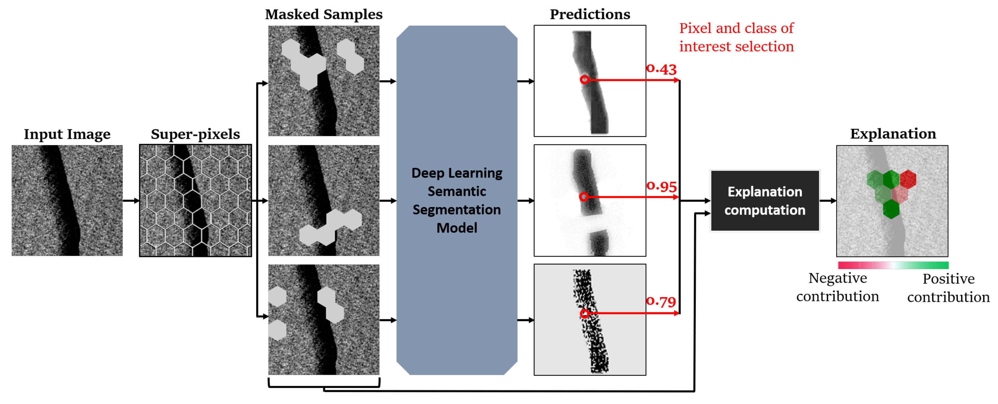
However, SHAP must be adapted to the semantic segmentation problem. To do so, we use an algorithm based on the KernelSHAP function [12], computing model-agnostic explanations linked to a specific input image. The proposed workflow is illustrated in Figure 11. It can be summarized by the following steps:
(1)
The first step aims at creating groups of pixels, or super-pixels, from the input image. The method result shows the contribution of each super-pixel in the model’s decision. Experiments have shown that relying on super-pixels of equal size and shape generates clearer explanations. Moreover, hexagonal super-pixels allow for a more natural explanation than square super-pixels, mainly due to the higher number of direct neighbors of each super-pixels. Thus, explanations presented in this paper rely on a grid of super-pixels shaped as a regular hexagon.
(2)
Then, masking is applied to the input image super-pixels in order to generate several masked samples, as shown in Figure 11. Note that masking super-pixels with the zero value is often considered in this step but is avoided in our case, as it would introduce ambiguity with the target (dark oil slicks). Thus, the explanations presented in this paper are based on a grid of super-pixels shaped like a regular hexagon.
(3)
The third step is to feed the resulting masked samples through a semantic black-box image segmentation model, which yields prediction probability maps for each sample.
(4)
The fourth step is to select the pixel and class of interest (e.g., the pixel highlighted in red in Figure 11 and the class “slick”), for which the explanation of the model decision is to be conducted.
(5)
After that, explanation computation based on Shapley values computation rules is applied [69], considering the mask and the pixel-level decision for every sample. In more detail, the Kernel SHAP algorithm estimates the impact of each super-pixel on the probability that the selected pixel belongs to the selected class (e.g., slick).
(6)
Finally, a heat map explanation is generated, highlighting the areas (super-pixel) of the input image that contributed positively (excited) and negatively (inhibited) to the model decision.
The result is obtained as an image, presenting the interpretation of the model decision for a given local (pixel level) classification. The interpretation (SHAP values) regarding a selected pixel (outlined in red on prediction matrices) is shown on the right in Figure 11. A SHAP value is assigned to each super-pixel, and these values are assigned to a color range. Red colors are attributed to a super-pixel decreasing the prediction value for the given class (inhibition, negative contribution to the class probability), and green colors are attributed to a super-pixel increasing this value (excitation, positive contribution to the class probability). The intensity of the color is directly linked to the amplitude of the SHAP value.

3. Results

In this section, the first part concerns the experiments conducted exclusively on SAR images using the selected deep neural network architectures. A presentation and comparison of the results are established. The second part discusses the fusion of SAR and wind information by the proposed Fuse-FC-DenseNet model. The identification of the most suitable approach is conducted with respect to the baseline model that relies on only the SAR information. The third part focuses on interpreting the results of both models (trained on SAR data alone and trained on SAR and wind speed data) by the adapted SHAP explanation method.
All comparisons and assessments of the results presented are based on the expertly selected test set presented in Section 2.2.3. It consists of SAR monitoring images of a real monitoring case with 214 slick instances of both types (spills and seeps) with various sizes, shapes, and slick characteristics.

3.1. Evaluation of SAR Data Experiments

3.1.1. Evaluation of Models Based on SAR Data

The evaluation of the proposed approaches is established on a test set of 214 instances of spill and seep, shown in Figure 4. The test set contains large SAR images (10,000 × 10,000 pixels) that are never seen during the training and validation of the models. It can also be noted that the test set belongs to an entirely new area (which was not included in the training/validation sets), implying a variation in the context. Thus, the performance of the models includes their generalization capabilities. The performance presented in Table 5 shows the instance and pixel level metrics of the enhanced FC-DenseNet and Mask-RCNN models. It shows that the improved FC-DenseNet model has a detection rate of 0.93 % , while the Mask-RCNN model has a rate of 0.83 % . However, the Mask-RCNN model has a slightly lower number of false alarms in the test set. In terms of pixel-level metrics, the improved FC-DenseNet significantly outperforms the Mask-RCNN in terms of IoU, precision, and recall.
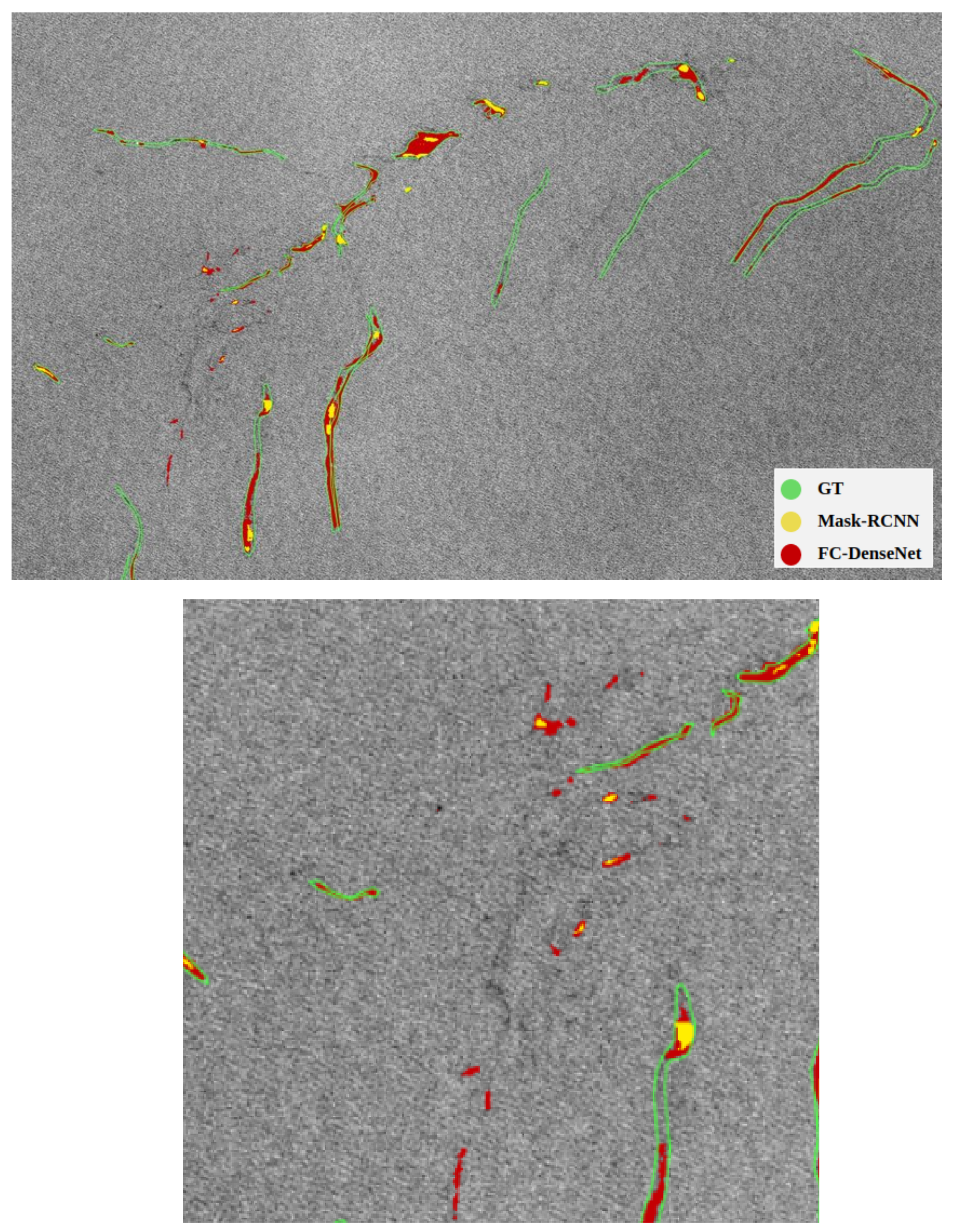
Figure 12 shows an illustration of the result of a test image containing different slicks. The predictions of both models are shown together with the ground truth. Predictions in red are placed under the yellow ones for a more trustworthy visualization. As we observe, Mask R-CNN fails to detect more annotated oil slicks and overlaps less with expert annotations (IoU 0.06 ). On the other hand, the improved version of FC-DenseNet covers the surface of slicks better (IoU 0.3 ). In terms of miss-detection rates, Mask R-CNN misses 2.3 times more slick instances than FC-DenseNet. More in-depth analysis shows that the spill miss-detection rate is around 40 % lower than the seep miss-detection rate for both models. This can be explained by the fact that the spill instance in our training set is higher than the seep instance. Regarding false alarm rates, the enhanced FC-DenseNet is higher and can be observed in the bottom part of Figure 12.
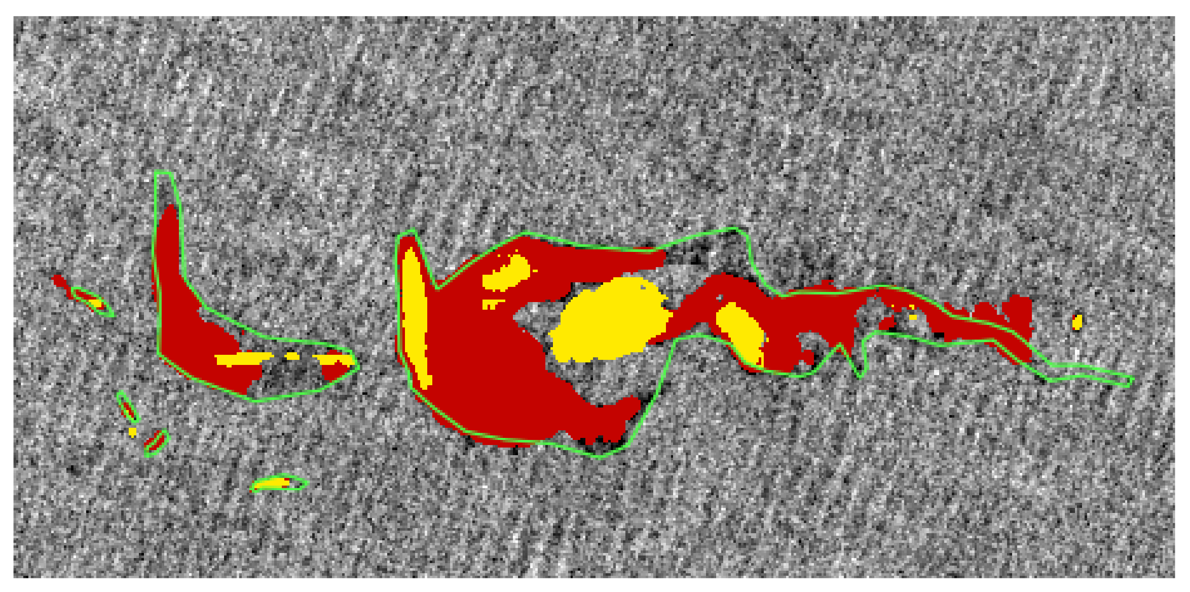
We observe that in the case of huge oil slicks, as seen in Figure 13, the improved version of the FC-DenseNet detection is fragmented. One general reason for this is the lack of large slicks in the training database. In addition, the detection is performed on image crops of 512 × 512 pixels for training and applied in a sliding window fashion on large test images. The models, therefore, only have a partial view of large slicks. In the situations where a slick extends over the entire crop area, its detection will be inhibited by the lack of contextual information. This could be combated by training on larger image crops but requires more memory on the GPUs.

3.1.2. Evaluation Based on Contextual Data

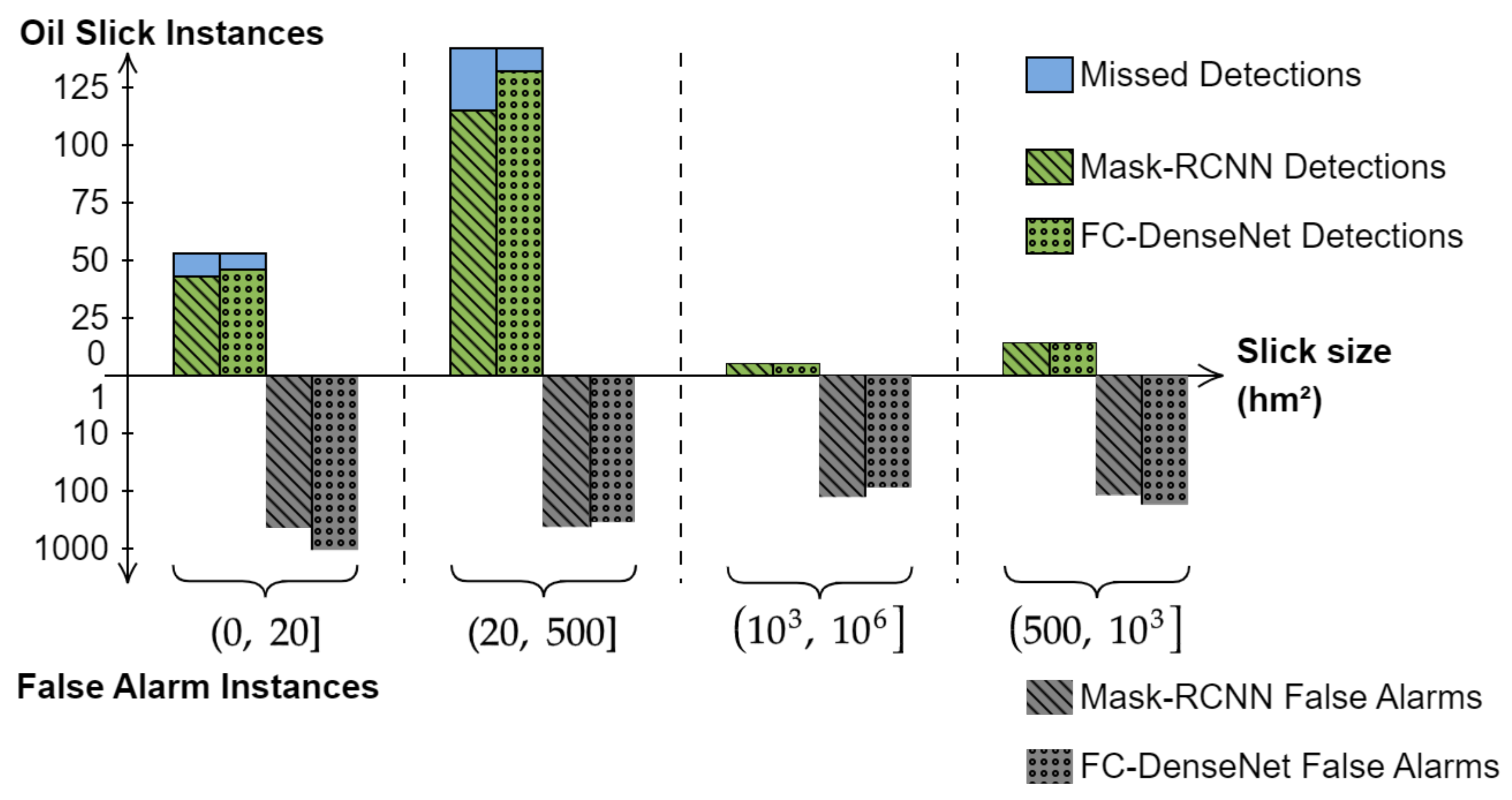
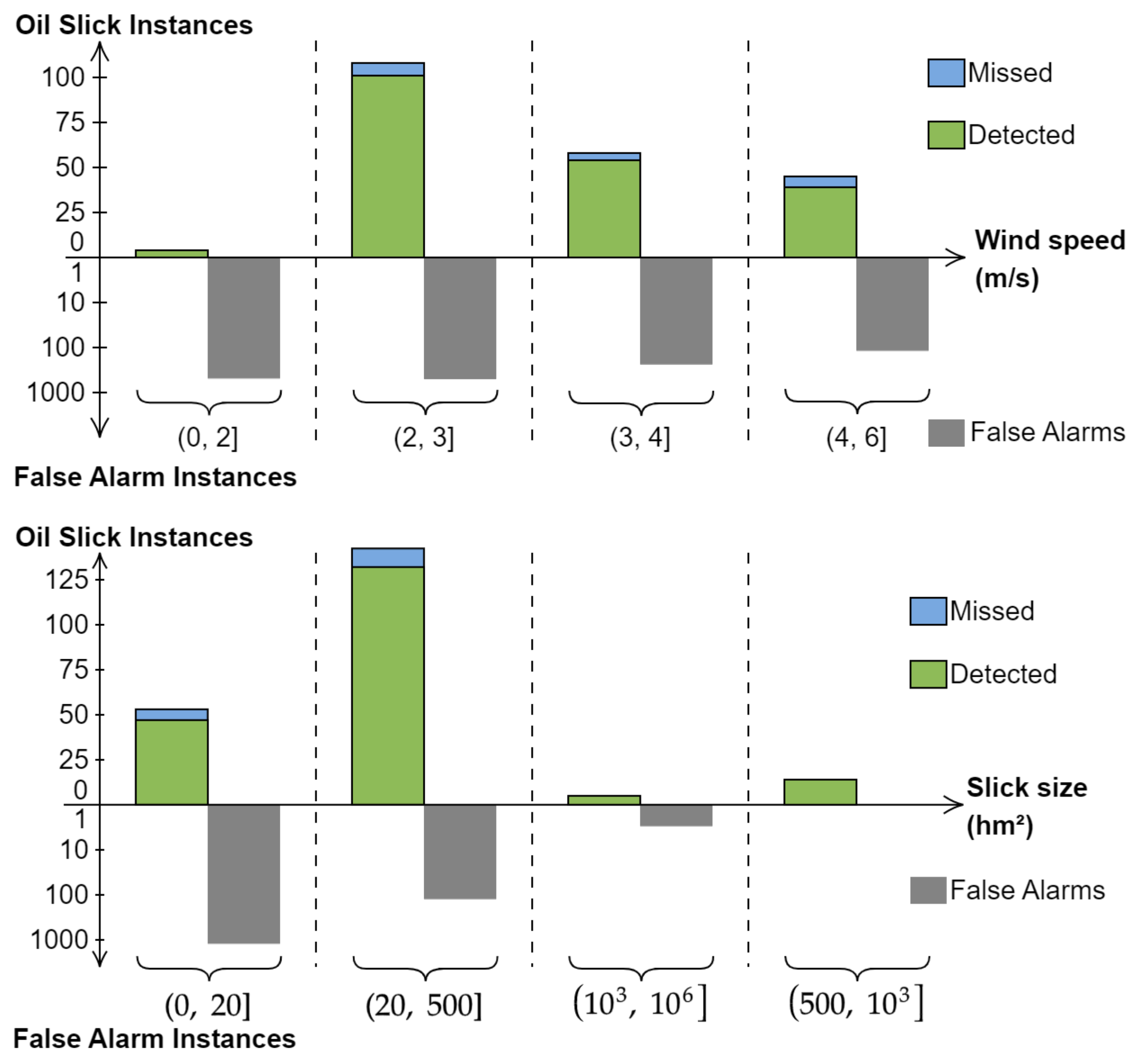
Figure 14 and Figure 15 show the results of the two approaches as a function of wind speed level and slick size. Similar general behaviors can be noted for both models, detecting slicks over the full range of wind speed and slick size. For both models, false detection areas are greater than 20 hm 2 and mostly correspond to windless areas, but their rate decreases as wind speed increases.
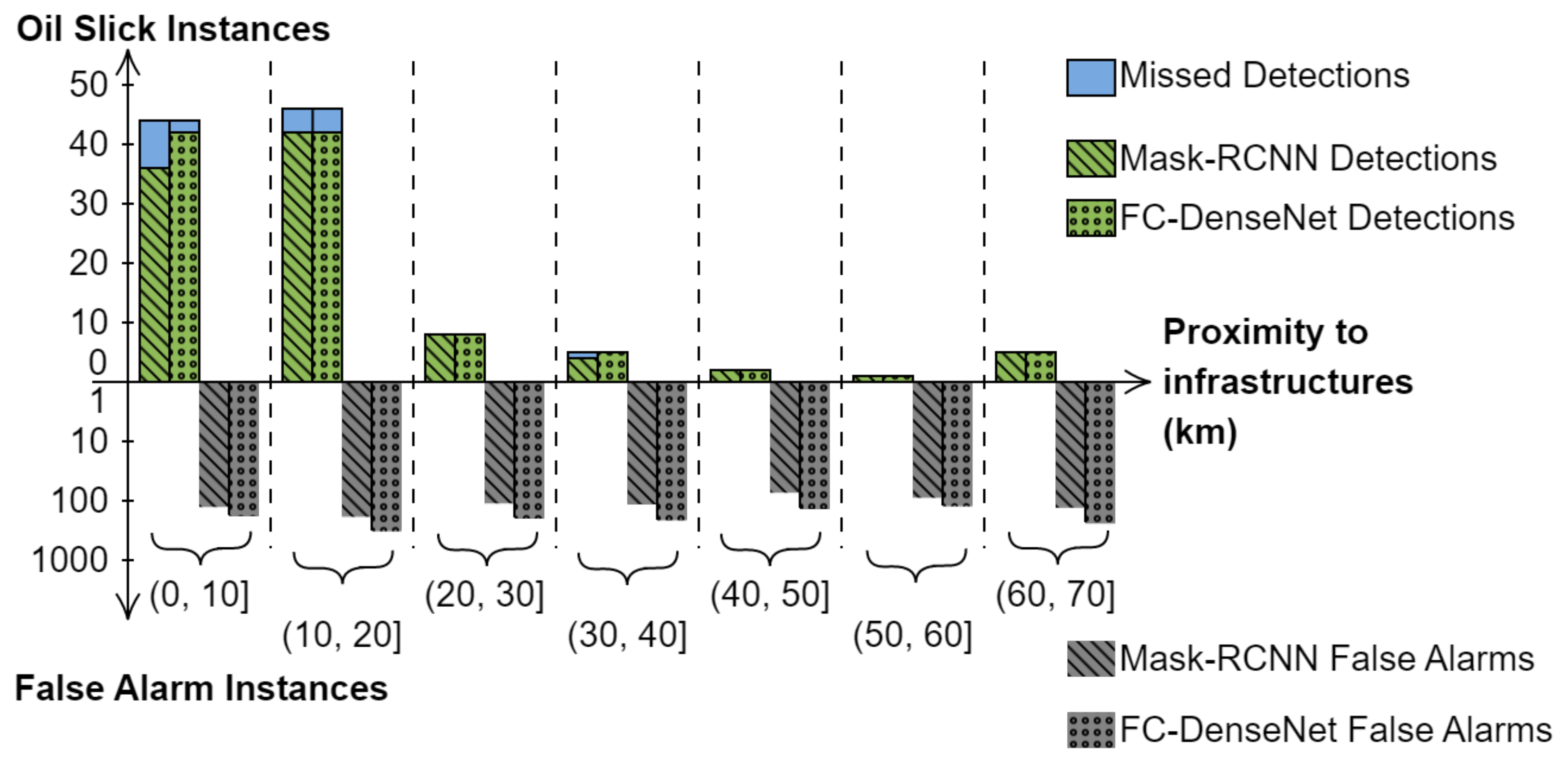
Figure 16 shows the distribution of the predictions of the two models regarding the proximity of the slicks (spill and seep) to infrastructure (ship, platform, pipeline, etc.). The information on proximity to infrastructure mainly relates to spill type, representing 150 instances in the test database. The improved version of FC-DenseNet model detects 149 / 150 spill instances, missing only one instance.
The first two bars ([0, 20] km) in Figure 16 shows both spill and seep instances, indicating that few slicks near the infrastructure are missed (blue). The R-CNN mask behaves similarly, detecting fewer slicks and missing some slicks farther from the infrastructure ([30, 40] km). The information on the proximity of the infrastructure represents relevant information for identifying the oil slick, notably the oil spill. This information serves as a reassurance to experts about the existence and type of slick.
As enhanced FC-DenseNet shows a better IoU value, reasonable detection rate, and miss-detection rate, this model is chosen as the baseline for the following experiments. An additional argument for this choice is also based on the fact that it is fully trained on the target data, unlike Mask R-CNN, which is pre-trained on other data.

3.2. Evaluation of Data Fusion Models

In this section, models conducting heterogeneous data fusion (SAR and wind speed information) are evaluated and compared against the SAR-based baseline model referred to as T S A R . Building upon the fusion strategies illustrated in Figure 5, several experiments have been performed. The most pertinent ones are reported in the following. T 0 corresponds to early fusion (the first arrow of Figure 5, only an upsampling of the wind maps is applied). Late fusion experiments correspond to the second arrow on the same figure, and we derive experiments T 1 , T 2 , T 3 , which systematically apply a subsampling (pooling) of the wind data to match the feature size of the SAR feature maps in later blocks. Those experiments differ in terms of feature extraction strategies on the wind information and fusion step positioning with respect to the SAR branch. Relevant experiment summaries are reported in Table 6, and the global results are presented in Table 7 and discussed in the following.

3.2.1. Early Fusion Experiment

When directly fusing SAR information with the upsampled wind data and providing this as a unified input to the model, the mitigated results are reported in Table 7. The number of good detection remains the same, and an 18% reduction of false detections is observed. This is consistent with the process of photo-interpreters using wind data to identify suspicious slicks and distinguish them from lookalikes. However, such an early fusion model reduces the IoU metric by 0.1 and also lowers precision and recall. The distribution of model detection as a function of wind speed and slick size is represented by the detection plots in Figure 17. Interpretations are similar to the baseline model.
Figure 18 shows a local comparison of the baseline SAR-based model and the early fusion strategy (displayed on top). The number of false detections of the baseline model is more noticeable, especially outside of the fine manual annotations.
Compared to the baseline model, the early fusion indicates a decrease in the IoU value. It may be noted that this limitation may be due to the manipulation of two data channels at the same scale. Meanwhile, the wind modality is highly interpolated. Extracting the fine resolution patterns do not seem appropriate. The fusion of wind data at a more appropriate scale should yield more insights.

3.2.2. Late Fusion Experiments

As shown in Table 7, in the case of late fusion at the block 2 levels (experiments T 1 and T 2 ), the detection rate (93.4%), IoU (0.31), precision (0.42), and recall (0.55) improve over the early fusion experiment T 0 and can reach or outperform the baseline. Further, by comparing the late fusion experiments, we notice that the later we fuse wind information with SAR, the lower the false detections at the price of a slight decrease in the number of good detection and a limited increase in the number of false detections. The slick IoU also decreases. However, the results are based only on selecting the most likely class between sea and slick and, therefore, they do not focus solely on slick probability levels, and further analysis is required.
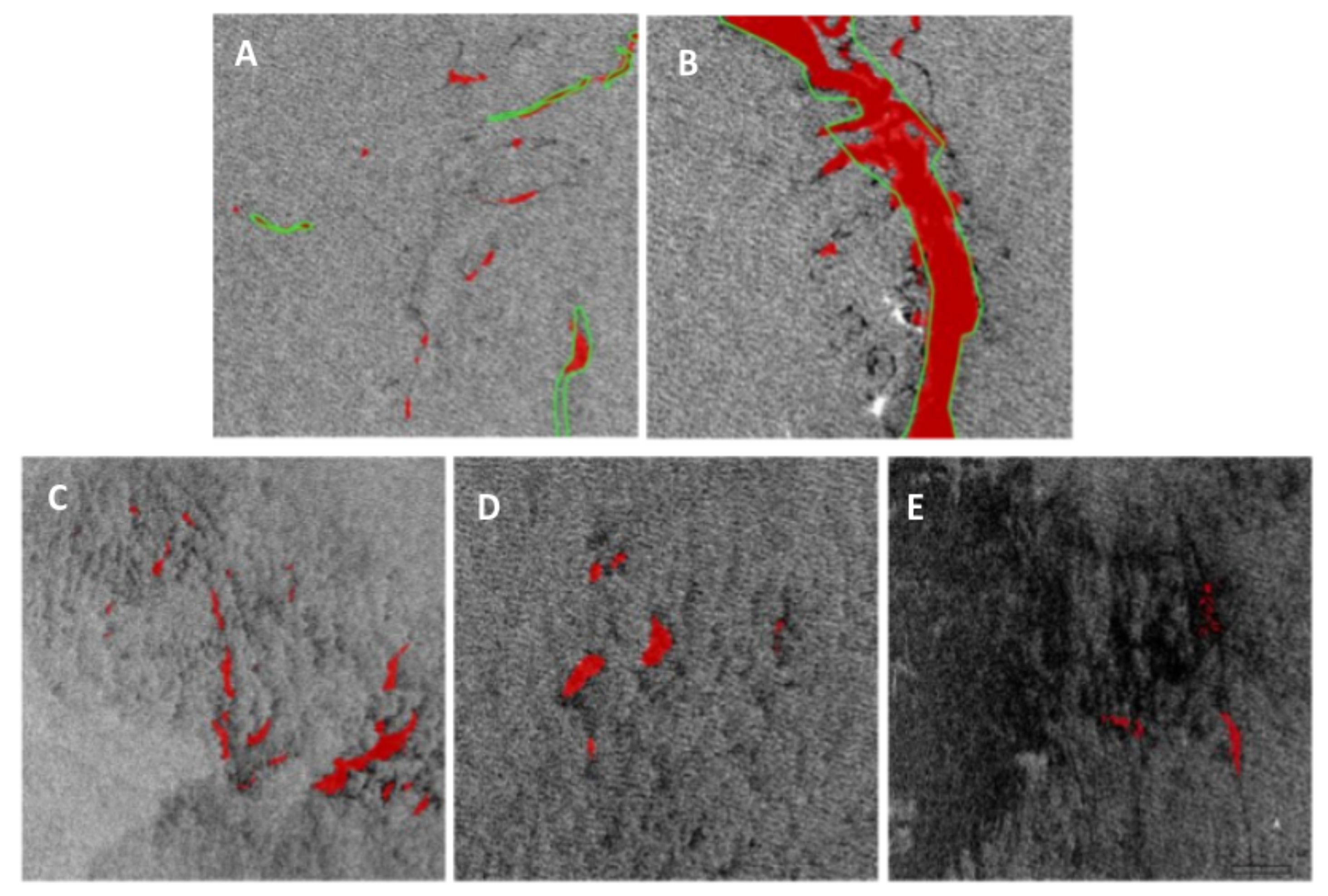
Regarding the number of false detections, we notice that they are often either around a large slick or grouped in the no-wind areas and fringed in small fragments such as Figure 19, showing an example of false detections of an improved version of the FC-DenseNet. A post-processing step of the dilation-erosion operation can be applied to minimize the number of false alarm instances.
Finally, for all the fusion experiments, a decrease in the number of false detections is observed. This then confirms the importance of wind speed for slick detection, especially for distinguishing slicks from lookalikes.

3.2.3. ROC Curves Analysis

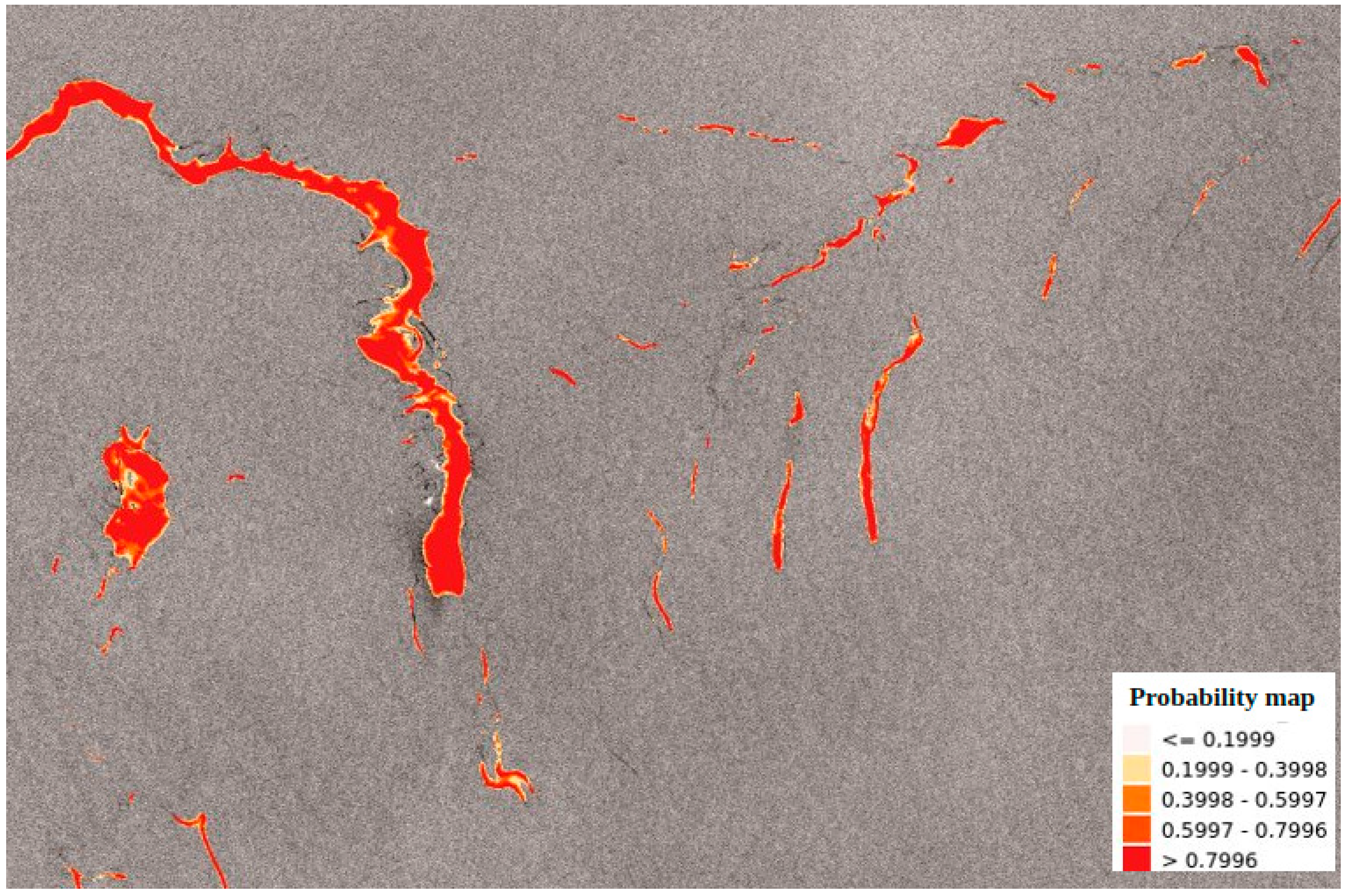
To better understand the prediction of the considered improved version of FC-DenseNet models, particularly their false detections, the slick probability maps outing from the model are analyzed. Figure 20 shows an example with a heat map representing the slick probability levels. One can visually observe that the slick inner surfaces generally have a high probability (red) and that the low probability values are always on the boundaries of the slicks (yellow). Given the quality of the annotation reported in Section 2.2, the IoU level remains strongly proportional to the quality of the ground truth boundary and cannot reach very high values.
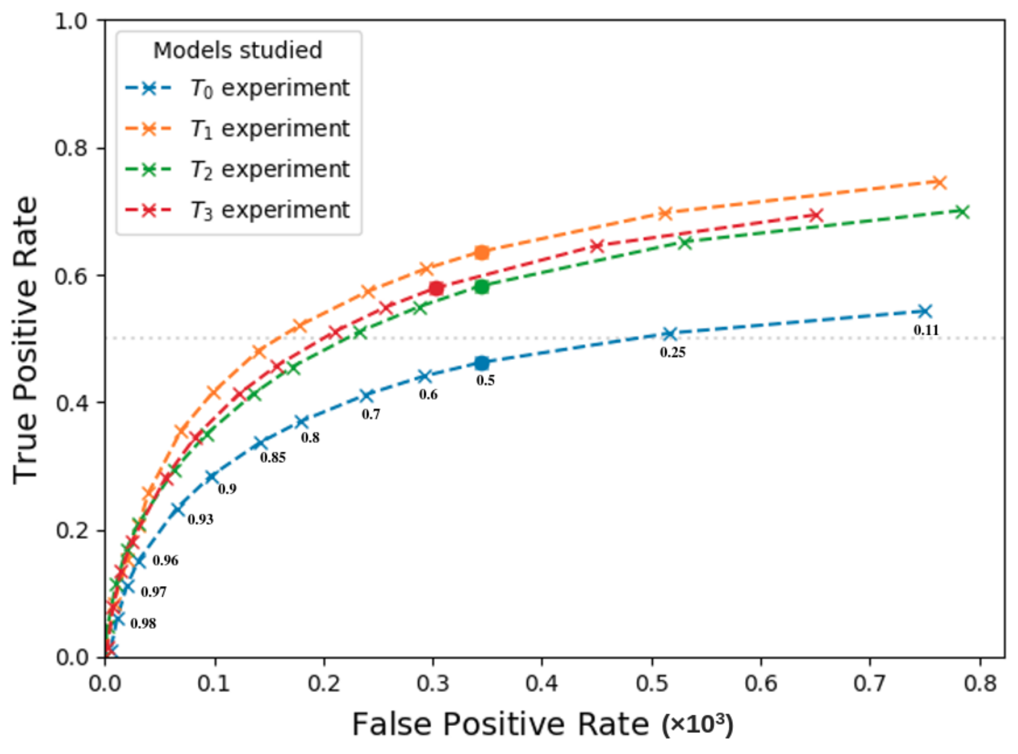
For a larger-scale investigation, these slick probability maps are considered to plot the ROC curves aggregating all the predictions on the test database for the different late fusion models. ROC curves for the fusion experiments are shown in Figure 21.
Experiment T 1 shows high values for each threshold measure compared to the other fusion experiments curves, which have a similar shape. It also shows a lower FPR for almost the entire range of TPR, we can assume that this fusion model provides the best segmentation quality.
Moreover, there is a noticeable gap between the late fusion experiments and the early fusion ones. This gap shows that late fusion is more appropriate in our context, as both input channels present too different characteristics to be considered at the same level in the architecture.
One can note that slick detection improvement can be made by selecting an adjusted threshold on the slick probability map instead of choosing the most probable class for every pixel. The threshold involves a different trade-off between TPR and FPR and thus can be decided by the domain experts.

3.3. SHAP Explanation

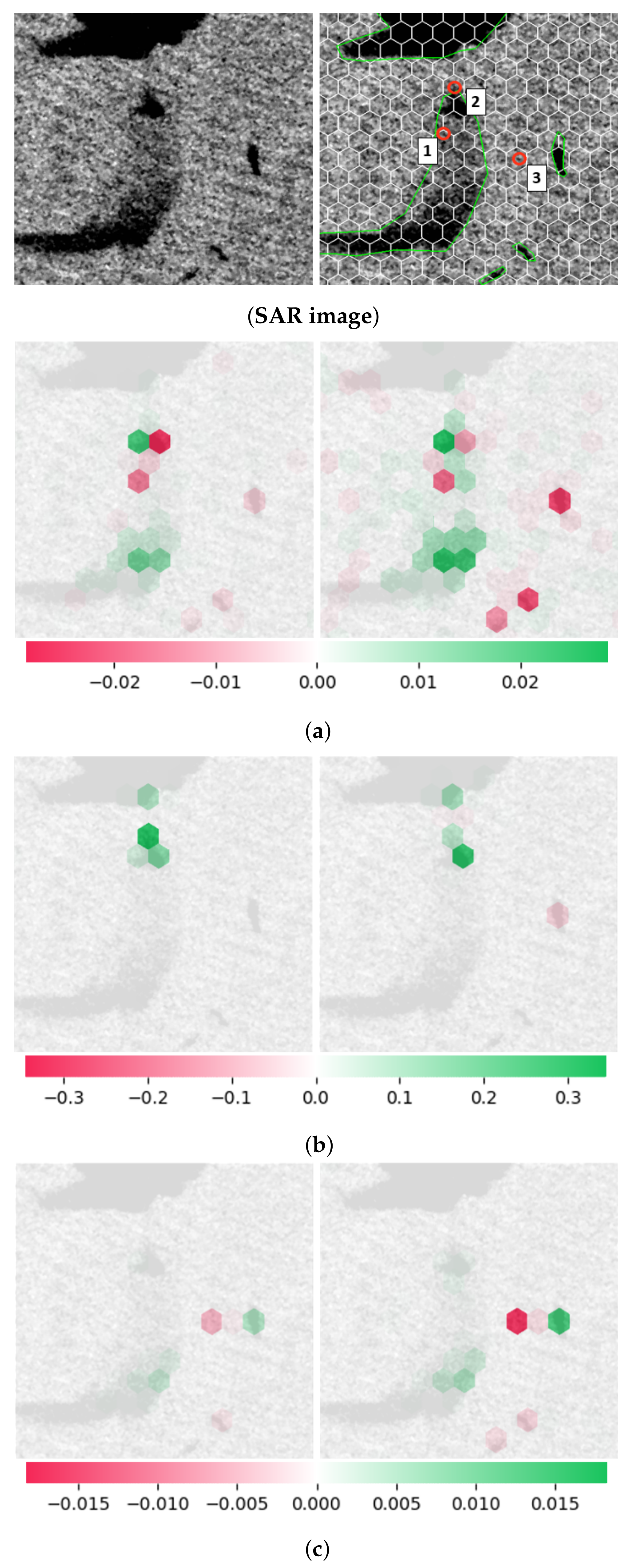
Explanation of the network decision processes can be made using the SHAP adaptation proposed in Section 2.3.2. This method is used to compare two models of interest: one corresponds to the T S A R experiment, and the other corresponds to the T 1 late fusion experiment. Then, based on the explanations obtained from the two model predictions on a varied set of the same pixels from the same input images, one can receive insights into the model behaviors and their differences in terms of the effective field of view and sensitivity to neighboring patterns. The following will focus on the three main observed behaviors illustrated in Figure 22, Figure 23 and Figure 24. These figures show the input images, a set of explained pixels (red circles), the applied features delimitation, and the explanation maps:
  • For a pixel classified as sea, as for explained pixels in Figure 22a,c and Figure 23a: the surface affecting the decision of the networks is large and depends on the presence of slicks (or lookalikes) in the entire image. Specifically, a general observation reveals that the prediction is mainly influenced by the presence of oil slicks in the vicinity of the explained pixel: a positive impact (reinforcing the classification of the pixel as slick) in the case of a relatively close slick and a negative one in the case of a distant slick. However, their contribution to the decision is extremely low and always countered by the considered pixel area. As a result, the prediction associated with the slick class is always close to 0 % .
  • For a pixel classified as slick, as for the explained pixel in Figure 22b, Figure 23c, and Figure 24b: the prediction is based on a limited area centered around the considered pixel. The maximal SHAP value in these cases is the highest observed (about 0.5). Typically, the network prediction for the pixel is impacted by one input feature containing mainly black pixels, which is enough to classify the pixel as a slick, with a probability above 80 % .
  • For a pixel located on a slick edge or within a narrow slick, as for the explained pixel in Figure 23b,d: networks tend to detect and base their decision on the slick edge or the narrow slick length. This shows that networks can detect the slick edges around the selected pixel in all observed images, which significantly influences their decision. The impact of each area containing a slick edge tends to decrease as the area moves away from the pixel.

4. Discussion

Based on the results obtained, we can confirm the ability of deep learning to detect both types of oil slicks (natural and anthropogenic) in a large-scale and real-world application, which contrasts with previous work dedicated to single types of oil slicks.
The result evaluation based solely on the SAR data shows a good detection rate but notable false alarms. The false alarms obtained can be divided into two categories: the first represents false alarms related to several lookalikes, such as low wind areas, algal blooms, and upwelling, as shown in Figure 19C–E, and the second represents false alarms related to small spots around an oil slick annotation, as shown in Figure 19A,B. These small oil slick patches, confirmed by photo-interpreters, are related to environmental effects, particularly meteorological conditions that influence the physicochemical properties of the oil slick, inducing its dispersion (fragmentation into droplets) and spreading process. These small oil slicks are also noticeable in Figure 15, where we can see the presence of false alarms ranging in size from 0 to 500 hm2.
One observation is that the ground truth annotation made by the photo-interpreters is not perfect and suffer from imprecise boundaries, as shown in Figure 2, revealing a diversity of annotations that position our detection task in a noisy reference context [70], as mentioned in Section 2.2. Hence the validation process requires a second pass of expertise on the large images to check the false alarms and eventually correct the annotations to integrate some false alarms as real slicks. We are thus, in a real context, allowing a continuous progression of the models and improvement of the annotations. This also becomes apparent in the prediction probability maps obtained by the models, as shown in Figure 20, where the lowest probabilities are always found on the slick boundaries. The imprecision of the annotation boundaries is apparent in the slick IoUs limited to 0.31 in Table 5 and also in the prediction probability maps obtained by the models, where the lowest probabilities are always found on the slick boundaries, as shown in Figure 20. Despite this, the semantic and instance segmentation models are quite capable of detecting slicks but suffer from false alarms.
To further reduce false alarms, we proposed Fuse-FC-DenseNet models that allow the fusion of wind speed and SAR data. Comparing the early and late fusion strategies using ROC curves shows that fusing wind data later in the models provides a satisfactory trade-off between good detection and false alarm rates. It can be noted that fusing wind speed data later in the model, approaching its resolution, provides better results than fusing too early, which causes the layers to learn inconsistent features, leading to undesired results. The obtained results with Fuse-FC-DenseNet have a better detection rate, and its detection better matches the photo interpretations (up to 93 % of the dataset targets are detected).
Late fusion experiments improve the performance while reducing false detections in the range of 14 % to 34 % . Regarding the late fusion experiments ( T 1 and T 3 ), the comparison is made based on the trade-off between good detection and false detection. T 3 shows a lower false alarm rate and detection rate than the single-modality (SAR) model results. This comparison is based on oil distribution in the dataset (214 oil instances). In the end, the choice of the best model is to be decided by the end-users to find the best compromise, taking into account the global costs that may include on-site verification flights.

Explainable Results

Going further, based on the comparison of the explanations presented in Section 3.3, it is possible to understand the effect of wind speed data on the model predictions. Figure 24a shows a lookalike that corresponds to waves. More precisely, one focuses on the explanation of the pixel of interest. This lookalike is detected as a slick only by the network that does not manage wind speed information ( T S A R ). The explanatory maps for both models show the impact of near-pixel areas on their decisions, increasing the probability of the pixel classification as a slick. However, the T 1 model that performs SAR and wind fusion gives more importance to contextual information: other dark patches in the image harm the classification of the considered pixel as a slick. The interpretation of this phenomenon is linked to the presence of wind speed data in the network decision process: the T 1 experiment can better differentiate slicks and lookalikes in this configuration, which makes contextual information more reliable. For all interpretations, the T 1 model shows a higher intensity of the SHAP value than the T S A R (red and green intensity in the SHAP images).
The proposed explanation method already provides valuable information to understand better and compare models. Its application to oil slick detection is interesting and aims to provide monitoring teams with additional information to help in the diagnosis of automated alarms. Several case studies and extensions of this approach are under consideration but are beyond the scope of this paper and will be discussed in future publications.

5. Conclusions

Deep learning for health, safety, and the environment is an active research trend, and oil spill monitoring is a relevant case study. To address this task, we demonstrate the interest in optimized semantic segmentation models based on the improved version of FC-Densenet and an instance segmentation approach transferred from another domain, Mask R-CNN. We evaluate and compare them relying on Sentinel-1 SAR imagery depending on domain expert photo-interpreters and taking into account contextual information regarding wind speed and proximity to human activities. First, we show the relevance of these approaches and propose a set of dedicated metrics that allow refined comparison of the models in various contextual situations in worldwide real-monitoring scenarios. Both models can detect slicks, but the improved version of FC-DenseNet has a better detection rate, and its detections better match the photo interpretations. Further, this paper shows the models applicability to detect oil slicks (both natural and anthropogenic), thus contrasting with previous work dedicated to a single slick type. In addition, we propose Fuse-FC-DenseNet model to fuse SAR and wind speed data to improve performances and diminish false alarm rates.
Compared to the baseline model, a decrease in false alarms is observed for all the fusion experiments. This then confirms the importance of wind speed for slick detection, especially for distinguishing slicks from lookalikes. The proposed Fuse-FC-DenseNet networks are capable of improving performance while reducing false detections in the range of 14 % to 34 % . As for human experts, such data fusion helps the models select relevant information to provide enhanced predictions and better distinguish oil slicks from lookalikes. The model predictions would be integrated into the industrial production pipeline to provide ready predictions to photo-interpreters. This will speed up the oil slick detection task and keep up with continuous sensor acquisition.
Finally, to offer ready-made predictions that are understandable by the photo-interpreters and enable human validation, we propose an extension of the SHAP explanation method that allows semantic segmentation predictions to be explained. It also allows a refined comparison of model behaviors on local decisions and their sensitivity to neighboring patterns in the data.
This work yields several insights, including the possibility of further studying explainability by extending analyses and explanations using the SHAP technique. In addition, different spatial organizations of the super-pixels can be tested, and analysis based on variability in the size of the contextual information can be established.
Another perspective may be to adapt the data fusion model further by introducing infrastructure position data as additional information during the learning process. The aim is to train the network to detect oil slicks and discriminate between spills and seeps.

Author Contributions

Investigation, E.A. and P.D.; Methodology; E.A., data curation; E.A. and H.C., Project administration; A.B., P.B., D.D. and A.C., Resources: D.D. and A.C., Software: E.A., Validation; P.B.; Supervision: P.B., A.B., A.C. and D.D., Writing—original draft: E.A. and P.D., Writing—review and editing; A.B. and D.D., Funding acquisition; A.C. and D.D. All authors have read and agreed to the published version of the manuscript.

Funding

This research was funded by TotalEnergies grant number FR00064703.

Data Availability Statement

Not applicable.

Acknowledgments

This work was carried out thanks to the ENVISAT and Sentinel-1 data provided by the European Space Agency.

Conflicts of Interest

Author E.A. received research grants from the company TotalEnergies. The funders have a role in the collection, partial preprocessing of the data, and the decision to publish the results.

Abbreviations

The following abbreviations are used in this manuscript:
AIArtificial Intelligence
EMElectroMagnetic
FAFalse Alarms
FC-DenseNetFully Convolutional DenseNet
GMFGeophysical Model Functions
Mask R-CNNMask Region Based Convolutional Neural Network
SARSynthetic Aperture Radar
SHAPSHapley Additive exPlanation
ROCReceiver Operating Characteristic
RSRemote Sensing

References

  1. Girard-Ardhuin, F.; Mercier, G.; Garello, R. Oil slick detection by SAR imagery: Potential and limitation. In Proceedings of the Oceans 2003. Celebrating the Past… Teaming Toward the Future (IEEE Cat. No. 03CH37492), San Diego, CA, USA, 22–26 September 2003; Volume 1, pp. 164–169. [Google Scholar]
  2. Alpers, W.; Holt, B.; Zeng, K. Oil spill detection by imaging radars: Challenges and pitfalls. Remote Sens. Environ. 2017, 201, 133–147. [Google Scholar] [CrossRef]
  3. Fingas, M.; Brown, C. Review of oil spill remote sensing. Mar. Pollut. Bull. 2014, 83, 9–23. [Google Scholar] [CrossRef] [PubMed] [Green Version]
  4. Brekke, C.; Solberg, A.H. Oil spill detection by satellite remote sensing. Remote Sens. Environ. 2005, 95, 1–13. [Google Scholar] [CrossRef]
  5. Angelliaume, S.; Dubois-Fernandez, P.C.; Jones, C.E.; Holt, B.; Minchew, B.; Amri, E.; Miegebielle, V. SAR imagery for detecting sea surface slicks: Performance assessment of polarization-dependent parameters. IEEE Trans. Geosci. Remote Sens. 2018, 56, 4237–4257. [Google Scholar] [CrossRef] [Green Version]
  6. Solberg, A.S.; Storvik, G.; Solberg, R.; Volden, E. Automatic detection of oil spills in ERS SAR images. IEEE Trans. Geosci. Remote Sens. 1999, 37, 1916–1924. [Google Scholar] [CrossRef] [Green Version]
  7. Espedal, H. Satellite SAR oil spill detection using wind history information. Int. J. Remote Sens. 1999, 20, 49–65. [Google Scholar] [CrossRef]
  8. Karathanassi, V.; Topouzelis, K.; Pavlakis, P.; Rokos, D. An object-oriented methodology to detect oil spills. Int. J. Remote Sens. 2006, 27, 5235–5251. [Google Scholar] [CrossRef]
  9. Nirchio, F.; Sorgente, M.; Giancaspro, A.; Biamino, W.; Parisato, E.; Ravera, R.; Trivero, P. Automatic detection of oil spills from SAR images. Int. J. Remote Sens. 2005, 26, 1157–1174. [Google Scholar] [CrossRef]
  10. Benoit, A.; Ghattas, B.; Amri, E.; Fournel, J.; Lambert, P. Deep learning for semantic segmentation. In Multi-Faceted Deep Learning; Springer: Berlin/Heidelberg, Germany, 2021. [Google Scholar]
  11. Krestenitis, M.; Orfanidis, G.; Ioannidis, K.; Avgerinakis, K.; Vrochidis, S.; Kompatsiaris, I. Oil spill identification from satellite images using deep neural networks. Remote Sens. 2019, 11, 1762. [Google Scholar] [CrossRef] [Green Version]
  12. Lundberg, S.; Lee, S.I. A unified approach to interpreting model predictions. arXiv 2017, arXiv:1705.07874. [Google Scholar]
  13. Li, X.; Nunziata, F.; Garcia, O. Oil spill detection from single-and multipolarization SAR imagery. In Reference Module in Earth Systems and Environmental Sciences; Elsevier: Amsterdam, The Netherlands, 2018. [Google Scholar]
  14. Espedal, H.; Hamre, T.; Wahl, T.; Sandven, S. Oil Spill Detection Using Satellite Based SAR, Pre-Operational Phase A; Technical Report; Nansen Environmental and Remote Sensing Center: Bergen, Norway, 1995. [Google Scholar]
  15. Wang, P.; Zhang, H.; Patel, V.M. SAR image despeckling using a convolutional neural network. IEEE Signal Process. Lett. 2017, 24, 1763–1767. [Google Scholar] [CrossRef] [Green Version]
  16. La, T.V.; Messager, C.; Honnorat, M.; Channelliere, C. Detection of convective systems through surface wind gust estimation based on Sentinel-1 images: A new approach. Atmos. Sci. Lett. 2018, 19, e863. [Google Scholar] [CrossRef]
  17. Najoui, Z.; Deffontaines, B.; Xavier, J.P.; Riazanoff, S.; Aurel, G. Wind Speed and instrument modes influence on the detectability of oil slicks using SAR images: A stochastic approach. Remote Sens. Environ. 2017. Available online: www-igm.univ-mlv.fr/~riazano/publications/NAJOUI_Zhour_thesis_paper1_Oil_slicks_detectability_from_SAR_images_draft31.pdf (accessed on 2 February 2022).
  18. Al-Ruzouq, R.; Gibril, M.B.A.; Shanableh, A.; Kais, A.; Hamed, O.; Al-Mansoori, S.; Khalil, M.A. Sensors, Features, and Machine Learning for Oil Spill Detection and Monitoring: A Review. Remote Sens. 2020, 12, 3338. [Google Scholar] [CrossRef]
  19. Chehresa, S.; Amirkhani, A.; Rezairad, G.A.; Mosavi, M.R. Optimum features selection for oil spill detection in SAR image. J. Indian Soc. Remote Sens. 2016, 44, 775–787. [Google Scholar] [CrossRef]
  20. Topouzelis, K.; Karathanassi, V.; Pavlakis, P.; Rokos, D. Detection and discrimination between oil spills and look-alike phenomena through neural networks. ISPRS J. Photogramm. Remote Sens. 2007, 62, 264–270. [Google Scholar] [CrossRef]
  21. Hamedianfar, A.; Barakat, A.; Gibril, M. Large-scale urban mapping using integrated geographic object-based image analysis and artificial bee colony optimization from worldview-3 data. Int. J. Remote Sens. 2019, 40, 6796–6821. [Google Scholar] [CrossRef]
  22. Guo, H.; Wu, D.; An, J. Discrimination of oil slicks and lookalikes in polarimetric SAR images using CNN. Sensors 2017, 17, 1837. [Google Scholar] [CrossRef] [Green Version]
  23. Yaohua, X.; Xudong, M. A sar oil spill image recognition method based on densenet convolutional neural network. In Proceedings of the 2019 International Conference on Robots & Intelligent System (ICRIS), Haikou, China, 15–16 June 2019; pp. 78–81. [Google Scholar]
  24. Chen, Y.; Li, Y.; Wang, J. An end-to-end oil-spill monitoring method for multisensory satellite images based on deep semantic segmentation. Sensors 2020, 20, 725. [Google Scholar] [CrossRef] [Green Version]
  25. Gallego, A.J.; Gil, P.; Pertusa, A.; Fisher, R. Segmentation of oil spills on side-looking airborne radar imagery with autoencoders. Sensors 2018, 18, 797. [Google Scholar] [CrossRef] [Green Version]
  26. Bianchi, F.M.; Espeseth, M.M.; Borch, N. Large-scale detection and categorization of oil spills from SAR images with deep learning. Remote Sens. 2020, 12, 2260. [Google Scholar] [CrossRef]
  27. Cantorna, D.; Dafonte, C.; Iglesias, A.; Arcay, B. Oil spill segmentation in SAR images using convolutional neural networks. A comparative analysis with clustering and logistic regression algorithms. Appl. Soft Comput. 2019, 84, 105716. [Google Scholar] [CrossRef]
  28. Emna, A.; Alexandre, B.; Bolon, P.; Véronique, M.; Bruno, C.; Georges, O. Offshore Oil Slicks Detection From SAR Images Through The Mask-RCNN Deep Learning Model. In Proceedings of the 2020 International Joint Conference on Neural Networks (IJCNN), Glasgow, UK, 19–24 July 2020; pp. 1–8. [Google Scholar]
  29. Amri, E.; Courteille, H.; Benoit, A.; Bolon, P.; Dubucq, D.; Poulain, G.; Credoz, A. Deep learning based automatic detection of offshore oil slicks using SAR data and contextual information. In Proceedings of the Remote Sensing of the Ocean, Sea Ice, Coastal Waters, and Large Water Regions 2021, Online, 13–17 September 2021; Volume 11857, pp. 35–42. [Google Scholar]
  30. Orfanidis, G.; Ioannidis, K.; Avgerinakis, K.; Vrochidis, S.; Kompatsiaris, I. A deep neural network for oil spill semantic segmentation in Sar images. In Proceedings of the 2018 25th IEEE International Conference on Image Processing (ICIP), Athens, Greece, 7–10 October 2018; pp. 3773–3777. [Google Scholar]
  31. Yu, X.; Zhang, H.; Luo, C.; Qi, H.; Ren, P. Oil spill segmentation via adversarial f-divergence learning. IEEE Trans. Geosci. Remote Sens. 2018, 56, 4973–4988. [Google Scholar] [CrossRef]
  32. He, K.; Gkioxari, G.; Dollár, P.; Girshick, R. Mask r-cnn. In Proceedings of the International Conference on Computer Vision (ICCV), Venice, Italy, 22–29 October 2017; pp. 2961–2969. [Google Scholar]
  33. Jégou, S.; Drozdzal, M.; Vazquez, D.; Romero, A.; Bengio, Y. The one hundred layers tiramisu: Fully convolutional densenets for semantic segmentation. In Proceedings of the IEEE Conference on Computer Vision and Pattern Recognition Workshops, Honolulu, HI, USA, 21–26 July 2017; pp. 11–19. [Google Scholar]
  34. Lin, T.; Maire, M.; Belongie, S.J.; Bourdev, L.D.; Girshick, R.B.; Hays, J.; Perona, P.; Ramanan, D.; Dollár, P.; Zitnick, C.L. Microsoft COCO: Common Objects in Context. In European Conference on Computer Vision; Springer: Berlin/Heidelberg, Germany, 2014. [Google Scholar]
  35. Abdulla, W. Mask R-CNN for Object Detection and Instance Segmentation on Keras and TensorFlow. 2017. Available online: https://github.com/matterport/Mask_RCNN (accessed on 2 February 2022).
  36. Lin, T.Y.; Goyal, P.; Girshick, R.; He, K.; Dollár, P. Focal loss for dense object detection. In Proceedings of the IEEE International Conference on Computer Vision, Venice, Italy, 22–29 October 2017; pp. 2980–2988. [Google Scholar]
  37. Huang, G.; Liu, Z.; Van Der Maaten, L.; Weinberger, K.Q. Densely connected convolutional networks. In Proceedings of the IEEE Conference on Computer Vision and Pattern Recognition, Honolulu, HI, USA, 21–26 July 2017; pp. 4700–4708. [Google Scholar]
  38. Ronneberger, O.; Fischer, P.; Brox, T. U-net: Convolutional networks for biomedical image segmentation. In Proceedings of the International Conference on Medical Image Computing and Computer-Assisted Intervention; Springer: Berlin/Heidelberg, Germany, 2015; pp. 234–241. [Google Scholar]
  39. Bottou, L. Stochastic gradient descent tricks. In Neural Networks: Tricks of the Trade; Springer: Berlin/Heidelberg, Germany, 2012; pp. 421–436. [Google Scholar]
  40. Kingma, D.P.; Ba, J. Adam: A method for stochastic optimization. arXiv 2014, arXiv:1412.6980. [Google Scholar]
  41. Sudre, C.H.; Li, W.; Vercauteren, T.; Ourselin, S.; Cardoso, M.J. Generalised dice overlap as a deep learning loss function for highly unbalanced segmentations. In Deep Learning in Medical Image Analysis and Multimodal Learning for Clinical Decision Support; Springer: Berlin/Heidelberg, Germany, 2017; pp. 240–248. [Google Scholar]
  42. Saxe, A.M.; McClelland, J.L.; Ganguli, S. Exact solutions to the nonlinear dynamics of learning in deep linear neural networks. arXiv 2013, arXiv:1312.6120. [Google Scholar]
  43. Krizhevsky, A.; Sutskever, I.; Hinton, G.E. Imagenet classification with deep convolutional neural networks. Adv. Neural Inf. Process. Syst. 2012, 25, 1097–1105. [Google Scholar] [CrossRef]
  44. Nair, V.; Hinton, G.E. Rectified linear units improve restricted boltzmann machines. In Proceedings of the International Conference on Machine Learning, Haifa, Israel, 21–24 June 2010. [Google Scholar]
  45. Bansal, N.; Chen, X.; Wang, Z. Can we gain more from orthogonality regularizations in training deep cnns? arXiv 2018, arXiv:1810.09102. [Google Scholar]
  46. Hénaff, O.J.; Simoncelli, E.P. Geodesics of learned representations. arXiv 2015, arXiv:1511.06394. [Google Scholar]
  47. Dong, C.; Loy, C.C.; He, K.; Tang, X. Image super-resolution using deep convolutional networks. IEEE Trans. Pattern Anal. Mach. Intell. 2015, 38, 295–307. [Google Scholar] [CrossRef] [Green Version]
  48. Valenzuela, G.R. Theories for the interaction of electromagnetic and oceanic waves—A review. Bound.-Layer Meteorol. 1978, 13, 61–85. [Google Scholar] [CrossRef]
  49. Goodman, R. Overview and future trends in oil spill remote sensing. Spill Sci. Technol. Bull. 1994, 1, 11–21. [Google Scholar] [CrossRef]
  50. Attema, E. An experimental campaign for the determination of the radar signature of the ocean at C-band. In Proceedings of the Third International Colloquium on Spectral Signatures of Objects in Remote Sensing, Les Arcs, France, 16–20 December 1986; pp. 791–799. [Google Scholar]
  51. Mouche, A. Sentinel-1 Ocean Wind Fields (OWI) Algorithm Definition; Sentinel-1 IPF Reference:(S1-TN-CLS-52-9049) Report; CLS: Brest, France, 2010; pp. 1–75. [Google Scholar]
  52. Freeman, A.; Curlander, J.C. Radiometric correction and calibration of SAR images. Photogramm. Eng. Remote Sens. 1989, 55, 1295–1301. [Google Scholar]
  53. Lihai, Y.; Jialong, G.; Kai, J.; Yang, W. Research on efficient calibration techniques for airborne SAR systems. In Proceedings of the 2009 2nd Asian-Pacific Conference on Synthetic Aperture Radar, Shanxi, China, 26–30 October 2009; pp. 266–269. [Google Scholar]
  54. Moreira, A.; Prats-Iraola, P.; Younis, M.; Krieger, G.; Hajnsek, I.; Papathanassiou, K.P. A tutorial on synthetic aperture radar. IEEE Geosci. Remote Sens. Mag. 2013, 1, 6–43. [Google Scholar] [CrossRef] [Green Version]
  55. Lillesand, T.; Kiefer, R.W.; Chipman, J. Remote Sensing and Image Interpretation; John Wiley & Sons: Hoboken, NJ, USA, 2015. [Google Scholar]
  56. Gao, F.; Xue, X.; Sun, J.; Wang, J.; Zhang, Y. A SAR image despeckling method based on two-dimensional S transform shrinkage. IEEE Trans. Geosci. Remote Sens. 2016, 54, 3025–3034. [Google Scholar] [CrossRef]
  57. Tong, S.; Liu, X.; Chen, Q.; Zhang, Z.; Xie, G. Multi-feature based ocean oil spill detection for polarimetric SAR data using random forest and the self-similarity parameter. Remote Sens. 2019, 11, 451. [Google Scholar] [CrossRef] [Green Version]
  58. Singha, S.; Vespe, M.; Trieschmann, O. Automatic Synthetic Aperture Radar based oil spill detection and performance estimation via a semi-automatic operational service benchmark. Mar. Pollut. Bull. 2013, 73, 199–209. [Google Scholar] [CrossRef]
  59. Wang, J.; Perez, L. The effectiveness of data augmentation in image classification using deep learning. Convolutional Neural Netw. Vis. Recognit. 2017, 11, 1–8. [Google Scholar]
  60. Powers, D.M. Evaluation: From precision, recall and F-measure to ROC, informedness, markedness and correlation. arXiv 2020, arXiv:2010.16061. [Google Scholar]
  61. Fawcett, T. An introduction to ROC analysis. Pattern Recognit. Lett. 2006, 27, 861–874. [Google Scholar] [CrossRef]
  62. Linardatos, P.; Papastefanopoulos, V.; Kotsiantis, S. Explainable ai: A review of machine learning interpretability methods. Entropy 2021, 23, 18. [Google Scholar] [CrossRef]
  63. Selvaraju, R.R.; Cogswell, M.; Das, A.; Vedantam, R.; Parikh, D.; Batra, D. Grad-cam: Visual explanations from deep networks via gradient-based localization. In Proceedings of the IEEE International Conference on Computer Vision, Venice, Italy, 22–29 October 2017; pp. 618–626. [Google Scholar]
  64. Vinogradova, K.; Dibrov, A.; Myers, G. Towards interpretable semantic segmentation via gradient-weighted class activation mapping (student abstract). In Proceedings of the AAAI Conference on Artificial Intelligence, New York, NY, USA, 7–12 February 2020; Volume 34, pp. 13943–13944. [Google Scholar]
  65. Ribeiro, M.T.; Singh, S.; Guestrin, C. “Why should i trust you?” Explaining the predictions of any classifier. In Proceedings of the 22nd ACM SIGKDD International Conference on Knowledge Discovery and Data Mining, San Francisco, CA, USA, 13–17 August 2016; pp. 1135–1144. [Google Scholar]
  66. Montavon, G.; Samek, W.; Müller, K.R. Methods for interpreting and understanding deep neural networks. Digit. Signal Process. 2018, 73, 1–15. [Google Scholar] [CrossRef]
  67. Van der Velden, B.H.; Janse, M.H.; Ragusi, M.A.; Loo, C.E.; Gilhuijs, K.G. Volumetric breast density estimation on MRI using explainable deep learning regression. Sci. Rep. 2020, 10, 18095. [Google Scholar] [CrossRef]
  68. Knapič, S.; Malhi, A.; Salujaa, R.; Främling, K. Explainable Artificial Intelligence for Human Decision-Support System in Medical Domain. arXiv 2021, arXiv:2105.02357. [Google Scholar]
  69. Shapley, L.S. 17. A Value for n-Person Games; Princeton University Press: Princeton, NJ, USA, 2016. [Google Scholar]
  70. Yu, S.; Chen, M.; Zhang, E.; Wu, J.; Yu, H.; Yang, Z.; Ma, L.; Gu, X.; Lu, W. Robustness study of noisy annotation in deep learning based medical image segmentation. Phys. Med. Biol. 2020, 65, 175007. [Google Scholar] [CrossRef]
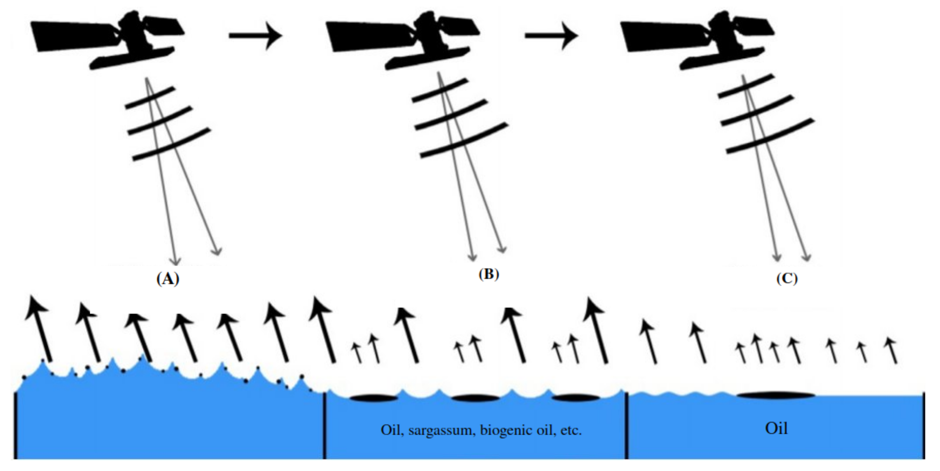
Figure 1. Illustration of SAR backscatter with different sea roughness. The wind conditions at the time of the data collection constrain the backscattered energy properties [13]. (A) represent strong winds (winds > 10 m/s), (B) represent ideal winds (7 m/s> Winds > 3 m/s) and (C) represent weak winds (winds < 3 m/s).
Remotesensing 14 03565 g001
Figure 2. Examples of oil slicks marked in yellow polygons (ai) and lookalike phenomena (jl) extracted from Sentinel-1 data.
Remotesensing 14 03565 g002
Figure 3. Mask R-CNN architecture. RPN stands for region Proposal Network, ROI stands for Region Of Interest.
Remotesensing 14 03565 g003
Figure 4. Architecture of the enhanced FC-DenseNet version. Orange blocks are convolutions, DB: dense blocks, TD: transitions down (2 times spatial downscale), TU: transitions up (2 times spatial upscale), C corresponds to the concatenation operation, and the dashed lines are skip connections.
Remotesensing 14 03565 g004
Figure 5. Fuse-FC-DenseNet architectures that fuse heterogeneous data, wind, and SAR information. The left branch is the wind branch, and the operations surrounded by red dotted lines are the different ways to fuse the wind speed information with the SAR information. (1) represents the early fusion, (2) represents the late fusion. The operations surrounded by red dotted lines are selected depending on the experiment.
Remotesensing 14 03565 g005
Figure 6. Location maps of the considered Areas Of Interest (AOI) captured from the Sentinel-1 sensor: (a,b) two areas of the Atlantic Ocean coast are located in Southern Africa (Nigeria and Namibia), (c) the Mediterranean Sea in Western Asia (Lebanon). The orange areas are used for training and validation, and the yellow area is used for testing.
Remotesensing 14 03565 g006
Figure 7. Example of slick annotation on a Sentinel-1 image on 21 January 2020 in the Nigeria area, where annotations are highlighted in green.
Remotesensing 14 03565 g007
Figure 8. Illustration of the wind information associated with the SAR image on 21 January 2020 in the Nigeria area. The SAR image with slicks and lookalike phenomena on the left, on the right, the associated wind speed data.
Remotesensing 14 03565 g008
Figure 9. Illustration of the position of infrastructures associated with the SAR image on 15 October 2018 in the Lebanon area. On the left, SAR image, on the right, the associated infrastructures position.
Remotesensing 14 03565 g009
Figure 10. Distribution of slick instances in the test dataset as a function of (from top to bottom) wind speed (m/s), slick size (hm2), and infrastructure proximity (km).
Remotesensing 14 03565 g010
Figure 11. Overview of SHAP adaptation to image semantic segmentation.
Remotesensing 14 03565 g011
Figure 12. An example of FC-DenseNet (red) and Mask R-CNN (yellow) prediction on Sentinel-1 images where green polygons represent manual slick annotations. A zoom in on an area of interest is placed at the bottom. Note that since Mask-RCNN is systematically within FC-DenseNet ones, Mask-RCNN masks are applied above FC-DenseNet to facilitate analysis.
Remotesensing 14 03565 g012
Figure 13. Sample of large slick and the corresponding prediction of FC-DenseNet and Mask R-CNN. Same legend as Figure 12.
Remotesensing 14 03565 g013
Figure 14. Detection performance of the improved version of FC-DenseNet and Mask R-CNN as a function of wind speed (m/s). Green bars represent good detection; blue shows missed detection. False alarms are represented by gray bars on a logarithmic scale.
Remotesensing 14 03565 g014
Figure 15. Detection performance of FC-DenseNet and Mask R-CNN as a function of ground truth size (hm2), same legend as Figure 14.
Remotesensing 14 03565 g015
Figure 16. Detection performance of FC-DenseNet and Mask R-CNN as a function of infrastructure proximity (km), same legend as Figure 14.
Remotesensing 14 03565 g016
Figure 17. Detection performance of Fuse-FC-DenseNet as a function of wind speed (m/s) and ground truth size (hm2), early fusion case.
Remotesensing 14 03565 g017
Figure 18. An example of the baseline SAR-based enhanced FC-DenseNet (red) and the early fusion version (blue) predictions to be compared with the green polygons representing the photo-interpretation slick annotation.
Remotesensing 14 03565 g018
Figure 19. False alarm samples for the improved baseline version of the FC-DenseNet model ( T S A R ). False alarms are marked in red and slick annotations are marked with green polygons. (A,B) represent false alarms around a slick, and (CE) represent other false alarms.
Remotesensing 14 03565 g019
Figure 20. Example of a prediction probability map of the improved version of FC-DenseNet model.
Remotesensing 14 03565 g020
Figure 21. ROC curves of fusion experiments ( T 0 , T 1 , T 2 , T 3 ). The threshold measurements marked on the blue curves are identical for all curves. The solid point represents the 0.5 threshold.
Remotesensing 14 03565 g021
Figure 22. Results of SHAP explanation function. (a) SHAP images for pixel number 1, classified as sea; (b) SHAP images for pixel number 2, classified as slick; (c) SHAP images for pixel number 3, classified as sea. (SAR image) right: SAR image, left: SAR image with a grid of white super-pixels representing the SHAP input. The ground truth is outlined in green and the pixels considered are numbered and circled in red. For SHAP image rows, right corresponds to the information obtained through the network T S A R , and left corresponds to information obtained through the T 1 experiment.
Remotesensing 14 03565 g022
Figure 23. Results of SHAP explanation function, showing effects of slick edges on networks. (a) SHAP images for pixel number 1, classified as sea; (b) SHAP images for pixel number 2, between slick and sea; (c) SHAP images for pixel number 3, classified as slick; (d) SHAP images for pixel number 4, between slick and sea. Similar legend to Figure 22.
Remotesensing 14 03565 g023
Figure 24. Results of SHAP explanation function, showing the difference between both studied experiments. (a) SHAP images for pixel number 1, classified as a slick by T S A R model and as sea by T 1 ; (b) SHAP images for pixel number 2, classified as slick. Same legend as Figure 22.
Remotesensing 14 03565 g024
Table 1. Range of wind speeds for oil slick detection according to the literature.
Wind Speed m/sReferenceYear
1.5 to 6[3]2014
2 to 7[16]2018
2.09 to 8.33[17]2017
3 to 7–10[4]2005
Table 2. Commonly used CNN models for oil slick detection.
ArchitectureCrop NumberImage SizeSpill & SeepTL
OFCN/UNet [26] 713160 × 160spill-
Fully CNNs [27]-128 × 128, 2048 × 2048spill-
Mask R-CNN [28,29] 9302512 × 512spill and seep
DeepLab [30] 6771252 × 609spill-
DeepLabv3+ [11] 1002321 × 321spill
AutoEncoders [25]-256 × 256, 384 × 384spill-
GANs [31]-256 × 256spill-
Table 3. Statistics of the training and validation dataset consisting of crops with a size of 512 × 512 pixels.
SpillSeepSeaTotal
Image crops number1.9642448603.068
Studied area surface (hm2)251,20021,9007,769,5008,042,600
Surface rate3.12%0.27%96.6%100%
Table 4. Statistics of the test dataset.
SpillSeepSeaTotal
Slick instances number15064-214
Studied area surface (hm2)49,77125,622267,112,507267,187,900
Surface rate3.12%0.27%96.6%100%
Table 5. Results of FC-DenseNet versus Mask R-CNN on a test set of 214 slicks.
MetricsFC-DenseNetMask R-CNN
Instance levelGood detection number198177
Miss-detection number1637
False-detection number16581103
Pixel levelIoU Slick0.30.06
Precision0.420.33
Recall0.530.06
Table 6. Experiment descriptions.
NameDescription
T S A R Enhanced FC-DenseNet baseline model relying exclusively on SAR data
T 0 Early fusion of upsampled wind data at the same level as the SAR data
T 1 Average pooling of the wind data and fusion with SAR data after dense block 2 (late fusion)
T 2 Average pooling and Denseblock applied to the wind data prior fusion with the SAR data after dense block 2 (late fusion)
T 3 Average pooling and Denseblock applied to the wind data prior fusion with the SAR data after dense block 3 (late fusion)
Table 7. Comparison of the FC-DenseNet results on a test set of 214 slicks using only SAR data with different data fusion models.
MetricsOnly SAREarly FusionLate Fusion
T S A R T 0 T 1 T 2 T 3
Instance levelGood detection number198198200201192
Miss-detection number1616141322
False-detection number16581357137614301094
Pixel levelIoU slick0.300.220.310.280.21
Precision0.420.350.420.380.24
Recall0.530.380.550.490.60
Publisher’s Note: MDPI stays neutral with regard to jurisdictional claims in published maps and institutional affiliations.