Article

Evaluation of Simulated AVIRIS-NG Imagery Using a Spectral Reconstruction Method for the Retrieval of Leaf Chlorophyll Content

1
Department of Physics, Indian Institute of Technology (BHU), Varanasi 221005, India
2
Remote Sensing Laboratory, Institute of Environment and Sustainable Development, Banaras Hindu University, Varanasi 221005, India
3
Geophysical Institute, University of Alaska Fairbanks, Fairbanks, AK 99775, USA
*
Author to whom correspondence should be addressed.
Remote Sens. 2022, 14(15), 3560; https://doi.org/10.3390/rs14153560
Submission received: 11 June 2022 / Revised: 20 July 2022 / Accepted: 21 July 2022 / Published: 25 July 2022
(This article belongs to the Special Issue Remote Sensing in Geomatics)

Abstract

:
The leaf chlorophyll content (LCC) is a vital parameter that indicates plant production, stress, and nutrient availability. It is critically needed for precision farming. There are several multispectral images available freely, but their applicability is restricted due to their low spectral resolution, whereas hyperspectral images which have high spectral resolution are very limited in availability. In this work, hyperspectral imagery (AVIRIS-NG) is simulated using a multispectral image (Sentinel-2) and a spectral reconstruction method, namely, the universal pattern decomposition method (UPDM). UPDM is a linear unmixing technique, which assumes that every pixel of an image can be decomposed as a linear composition of different classes present in that pixel. The simulated AVIRIS-NG was very similar to the original image, and its applicability in estimating LCC was further verified by using the ground based measurements, which showed a good correlation value (R = 0.65). The simulated image was further classified using a spectral angle mapper (SAM), and an accuracy of 87.4% was obtained, moreover a receiver operating characteristic (ROC) curve for the classifier was also plotted, and the area under the curve (AUC) was calculated with values greater than 0.9. The obtained results suggest that simulated AVIRIS-NG is quite useful and could be used for vegetation parameter retrieval.

Graphical Abstract

1. Introduction

Remote sensing has become significant in Earth science, observation, research, and solving environmental problems. Many satellites and unmanned aerial vehicles (UAV) are available now to help us understand the Earth’s surroundings. Sensors collect data ranging from visible to microwave frequencies in the electromagnetic spectrum. A wide range of sensors, including multispectral sensors (MSS) and hyperspectral sensors (HSS), give information in different spectral resolutions. However, MSS is limited in use because of its lower spectral resolution than HSS. The former gives information in around 10–15 spectral bands, whereas the latter provides information in the order of 100 bands. Hyperspectral data have far more information than multispectral data, thus dramatically expanding the variety of remote sensing applications [1]. HS imagery provides detailed information due to the narrow bandwidth but is scarcely available due to the high data acquisition cost. At present, there are only a few space-borne hyperspectral sensors available. On the other hand, widely available multispectral data can be used to simulate or construct hyperspectral data, particularly in situations where the latter are required but difficult to obtain.
There is extensive use of data simulation in the remote sensing field to generate images for virtual or novel sensors in the design stage. Simulated data can also be used to assess spatial properties important to a specific study and compared with the spectra obtained from a sensor [2]. Data simulation is frequently used to assess the impact of various spectral or spatial resolutions in specific applications to determine the best resolution for a given problem [3,4]. Some researchers assessed the applicability of linear spectral unmixing to different degrees of spatial resolution by simulating hyperspectral data with varied spatial resolution. In contrast, others assessed the impact of spatial and spectral resolution on vegetation categorization. Furthermore, this method has found its usage in assessing and testing new algorithms in HS remote sensing, such as target detection and identification [5].
For this study, the vegetation parameter of interest was leaf chlorophyll content (LCC), a biochemical parameter that gives information about the pigment level and individual vegetation’s nutrition. Thus, creating a thorough and accurate image for crop development status requires a quantitative estimation of crop leaf chlorophyll concentration. With the change in stages of the vegetation, whenever exposed to stresses, the LCC value also changes. The change in the pigment level determines vegetation health. As a result, determining its level is required to query plant stress and nutritional status to maximize crop yield [6,7]. Traditional approaches for estimating LCC are costly, time-consuming, and damaging. Hyperspectral remote sensing provides a nondestructive and scalable monitoring strategy. Thus, investigating vegetation’s spectra using hyperspectral remote sensing yields promising findings for retrieving this biochemical parameter [8].
Various approaches are used to estimate the biochemical composition of the vegetation. The most straightforward method is to directly build a statistical relationship between the in-situ parameter value and canopy reflectance obtained using aerial or satellite sensors [9,10,11]. The most extensively used semiempirical methods for estimating LCC are vegetation index-based and multivariate statistical approaches [12]. The vegetation index (VI) is a linear or nonlinear combination of reflectance at different wavelengths used to indicate information about vegetation. VIs exploit reflectance/absorption values in the visible and near-infrared (NIR) regions of the electromagnetic spectrum. The benefit of utilizing VIs is that they improve spectral information by identifying variations caused by physiological and morphological factors [13]. Physical modeling for estimating leaf biochemical contents has made significant progress. Numerical inversion of radiative transfer (RT) models such as PROSPECT and LEAFMOD have been used to predict LCC [14,15,16,17]. Several researchers have also worked with enhanced learning algorithms combined with VIs for the retrieval of vegetation parameters in order to avoid the mathematical complexity of physical models [18,19,20].
The universal pattern decomposition method (UPDM) is a spectral reconstruction approach based on the spectral unmixing method; it is a modified version of the pattern decomposition method [21]. UPDM is a sensor-independent technique in which each satellite pixel is expressed as the linear sum of fixed, standard spectral patterns for significant classes, and the same normalized spectral patterns can be used for different solar-reflected spectral satellite sensors. There have been studies where UPDM has been used to generate different HSS data for different sensors using MS data. Zhang et al. suggested a spectral response technique for hyperspectral data simulation from Landsat 7 Enhanced Thematic Mapper Plus (ETM+) and Moderate Resolution Imaging Spectroradiometer (MODIS) data that employed the UPDM. Liu et al. used the same method to recreate 106 hyperspectral bands from the EO-1 Advance Land Imager (ALI) multispectral bands using normal ground spectra of water, vegetation, and soil. Badola et al. used UPDM to reconstruct Airborne Visible-Infrared Imaging Spectrometer—Next Generation (AVIRIS-NG) imagery from Sentinel-2 for improved wildfire fuel mapping in Boreal, Alaska. The spectral reconstruction technique has also found its application in mineral mapping [5,22,23]. Muramatsu et al. used UPDM for vegetation type mapping from ALOS/AVNIR-2 and PRISM data. Until now, UPDM has proven its usefulness in various fields for mapping and classification purposes; however, the efficiency of reconstructed HS imagery using UPDM for retrieving vegetation parameters with application in agriculture has yet to be explored.
In the presented work, we used UPDM to simulate AVIRIS-NG imagery using Sentinel-2 for a region in the Gujarat district that contains mainly agricultural areas to expand the use of the UPDM method in the retrieval of vegetation parameters. The simulated data were evaluated visually and statistically, and then further verified for the LCC retrieval of various crops in different vegetative stages.

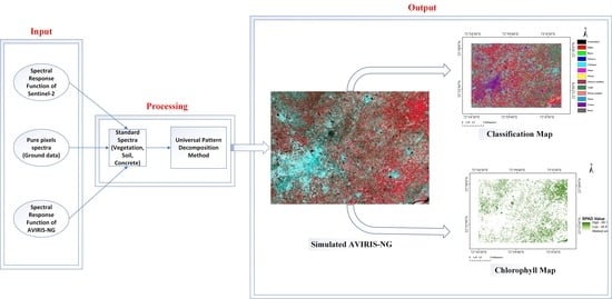
2. Materials and Methods

2.1. Study Area and Data Acquisition

This study was conducted on the AVIRIS-NG India campaign site in Anand district, Gujarat, located in the western part of India. The geographical area of the district lies between 72°00′–72°99′N and 22°46′–22°56′E with an elevation of 39 m, making it the 20th largest district that covers an area of 2951 km2. The annual rainfall records in the district vary between 286.9 mm and 1693.4 mm; during the southwest monsoon, the highest rainfall recorded from June to September is 687 mm. Different types of soil such as black cotton, mixed red and black, residual sandy, alluvial, and lateritic are found in the district. However, the major soil found in the study area is Goradu (gravelly) and black. Anand district is mainly covered with heterogeneous agricultural crops such as wheat, maize, sorghum, tobacco, Amaranthus, tomato, and chickpea. Tobacco, rice, and wheat are the major growing crops in the study area. Rigorous field sampling was performed during the flight overpass of AVIRIS-NG in the month of March 2018 [22,23].

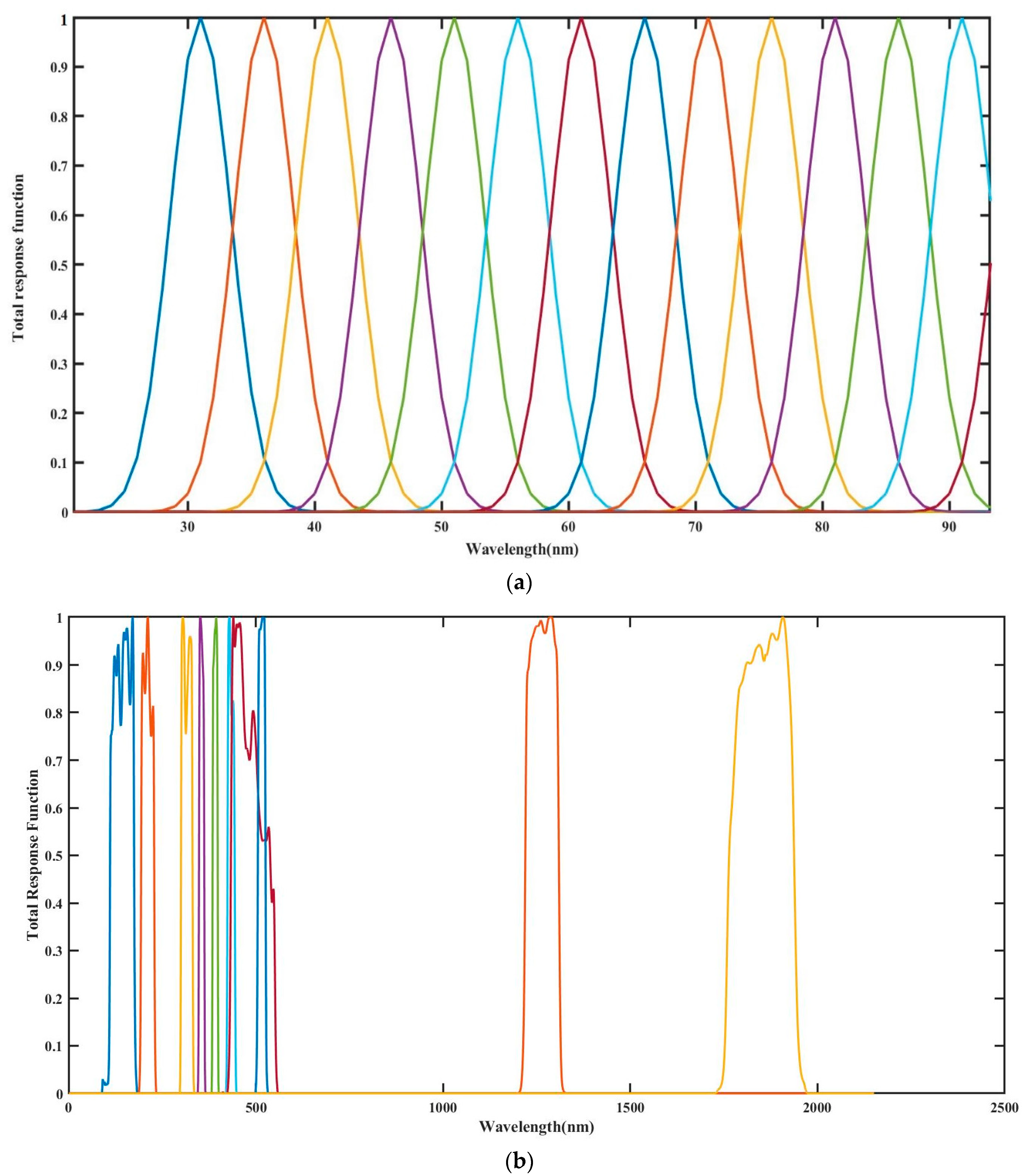
2.2. Remotely Sensed Data

2.2.1. Hyperspectral Data

The second AVIRIS-NG Indian campaign was held from 26–28 March 2018. The collected level-2 surface reflectance AVIRIS—Next Generation (NG) scene was downloaded from the VEDAS-SAC (source: https://vedas.sac.gov.in/aviris/) geoportal assessed on 8 September 2018. The downloaded scene includes the agricultural area of the Anand district, Gujarat [24,25]. AVIRIS-NG mission is a collaboration of NASA and ISRO. It is also known as a push broom spectral mapping system, designed for high-performance spectroscopy with high signal-to-noise ratio (SNR) values. AVIRIS-NG, also known as a hyperspectral imaging spectrometer, collects 425 contiguous bands with 5 nm spatial resolution. The wavelength ranges from 0.38 to 2.51 μm VNIR (400–100 nm) and SWIR (970–2500 nm) regions with 8.1 m spatial resolution [26]. AVIRIS-NG was developed as the next generation of the classic Airborne Visible Infrared Imaging Spectrometer. It measures the data at 5 nm sampling intervals with high SNR >2000 at 600 nm and >1000 at 2200 nm. Due to its narrow contiguous bands, the most applicable and precise information can be retrieved for any location. The accuracy of AVIRIS-NG was noted as 95% with an FOV (field of view) of 34° and IFOV (instantaneous field of view) of 1 m rad (https://aviris-ng.jpl.nasa.gov/ accessed on 10 June 2022), along with a resolution of ground sampling distance (GSD) of 4–8 m at a flight elevation of 4–8 km [27]. Data can be downloaded from the ‘Vedas’ site in both radiance and reflectance format. Due to the presence of various types of atmosphere aerosols, it makes the data vulnerable to distortions and need to be preprocessed using various atmospheric correction methods. Presented AVIRIS-NG data were preprocessed, and current L1 products were used (radiance to reflectance).

2.2.2. Multispectral Data

Sentinel-2 images acquired on 28 March 2018 for the study site were downloaded from the Copernicus open access hub of ESA (source: https://scihub.copernicus.eu/dhus/#/home) assessed on 16 October 2021. The original L1C (top-of-atmosphere) product was converted to L2A (bottom-of-atmosphere) reflectance using the Sen2cor processor. Sentinel-2 has a multispectral imager (MSI) that captures images in 13 bands with different resolutions i.e., 10 m, 20 m, and 60 m. The bands B2 (blue), B3 (green), B4 (red), and B8 (NIR) have a spatial resolution of 10 m, while bands B5 (red edge), B6, B7, B8a (NIR), B11, and B12 (SWIR) have a pixel size of 20 m. The bands B1 (coastal aerosol) and B10 (cirrus) have 60 m resolution. For this study, bands B1 and B10 were removed, and the remaining bands were resampled to a pixel size of 10 m; all bands were stacked, and the study area was clipped. The analysis of multispectral imagery was performed in SNAP 8.0.

2.2.3. Ground Data

The pure spectra for various vegetation were used from the spectral library generated during the field campaign i.e., 26–28 March 2018. In the sampling, spectra of different species were collected at different vegetative stages. The field spectra were taken with a high-resolution ASD FieldSpec4 spectroradiometer. The spectral range of the radiometer covers wavelengths ranging from 350 to 2500 nm with a sampling rate of 0.2 s per spectrum. It has different spectral resolutions at different wavelengths, 3 nm in the very short IR and 10 nm in the far-IR wavelengths, which are resampled to 1 nm. The device records spectra on the basis of information provided by 2151 bands. The leaf chlorophyll content was collected from Soil Plant Analysis Development (SPAD) during a field campaign held from 26–28 March 2018. The device measures the transmittance in the red and infrared regions and gives LCC values to three significant figures [28]. Extensive sampling was performed to collect data such as stage, soil condition, chlorophyll content, and plant height, coinciding with the AVIRIS-NG flight overpass dates.

2.3. Simulating AVIRIS-NG from Sentinel-2 Using UPDM

2.3.1. Calculating Standard Spectra

The reflectance from a pixel’s FOV gives the combined spectra of classes in the pixel. The study site contained mostly agricultural fields, harvested land, bare soil, and some urban areas, as shown in Figure 1. We chose vegetation, bare soil, and urban area as three primary classes/endmembers to be given to the algorithm. For urban area, a spectrum of concrete was downloaded from the USGS library and used in the process of simulation. The concrete spectrum had the exact spectral resolution and wavelength range of vegetation and soil spectra. The other two classes (vegetation and soil) were taken from the spectral library generated during field sampling.
The standard spectra for each class, i.e., vegetation, soil, and concrete, were calculated by convolving the pure spectra with the spectral response function (SRF) of the sensors to normalize them. The SRF for Sentinel-2 was downloaded from the ESA document library, whereas the SRF for AVIRIS-NG was calculated. The full width at half maximum (FWHM) values for each band are available; in order to calculate SRF for AVIRIS-NG sensors, a Gaussian function (g) for the ith band was calculated as follows:
g λ i ¯ , σ i = e x p λ i ¯ λ 2 2 σ i 2 .
The FWHM of each band was used to get the bandwidth.
σ i = F W H M 2 2 l n 2 ,
where λ ¯ is the central wavelength, σ is the bandwidth, and λ is the wavelength. Figure 2a,b show the SRFs of AVIRIS-NG and Sentinel-2 sensors.

2.3.2. Spectral Unmixing

The method used for the study was UPDM, which is a sensor-independent spectral reconstruction method. UPDM is a multidimensional analysis, whose working is similar to the spectral unmixing method. The reflectance of each pixel is decomposed into the summation of standard spectra of various significant classes. The three major classes present in the study site are vegetation, concrete, and soil. Under the vegetation class, different agricultural crops are present, which was identified and noted during data sampling. Buildings and road come under the concrete class, and harvested agricultural, plowed field, and bare soil area come under the soil class. These three endmembers were used in UPDM to generate the AVIRIS-NG image for the entire area.
R i = P i v C v + P i s C s + P i c C c ,
where Ri is the reflectance of a particular pixel in the band i measured by any sensor, Cv, Cs, and Cc are the decomposition coefficients for vegetation (v), soil (s), and concrete (c), respectively, and Piv, Pis, and Pic are the respective normalized standard spectra for the mentioned classes.
Mathematically, UPDM can be expressed in the form of matrices as shown below.
R = P × C.
R 1 R 2 R n = P 1 v P 1 s P 1 c P 2 v P 2 s P 2 c P n v P n s P n c C V C S C C ,
where n is the number of bands, and R1, R2, …, Rn is the reflectance value of a pixel in each band. P is the standard pattern matrix of order n × 3, and it is unique for every sensor. C is the decomposition coefficient matrix.
For a multispectral sensor, Equation (2) becomes
R m = P m C m .
Decomposition coefficient matrices (Cm) were calculated from Sentinel-2 using UPDM. Cm calculates the fraction of class in a pixel. This matrix would remain same for simulated hyperspectral data due to its sensor independent property. R m is the reflectance value matrix for Sentinel-2 image, and P m is the standard spectral matrix for major classes (v, s, c). Cm is obtained by minimizing the sum of squared error.
C m = P m T . P m 1 . P m T . P m .
Furthermore, for the simulation of HS spectra,
R h = P h C h .
Cm replaces Ch in the above equation using Equation (5). The spatial resolution of simulated HS data would have the same value as that of MS data, which is why the coefficient matrix does not change for both sensors.
R h =   P h . P m T . P m 1 . P m T . P m ,
where Rh is the resultant simulated HS reflectance matrix, and it contains 425 simulated bands of AVIRIS-NG. The simulation was conducted in MatLab. Figure 3 and Figure 4 show the comparison of a vegetation and soil spectra. Some of the noisy bands were removed from both the spectra due to one or another kind of scattering or absorption, e.g., bands 196–210 and 290–309 were removed due to water vapor absorption bands, whereas bands 408–425 were removed due to strong water vapor and methane absorption.

2.4. Classification Using Spectral Angle Mapper (SAM)

Different classes in the generated HS image were identified using SAM, which identifies unknown pixels on the basis of the degree of similarity between their spectral profiles and those of the references. SAM considers the reference classes and spectra as vectors in a space that has dimensions equal to the number of bands.
α = cos 1 X . Y X 2 Y 2   ,
where α is the angle between vectors (references and original spectra), X is the original spectrum, and Y is the reference spectrum. Different values of α were given to run the classification; for α = 0.5 radian, the classifier gave the best results.
Classification distinguished 12 different classes in the simulated imagery including different vegetation species, urban, water, and road (Figure 5). The ground-truth image was used to classify the image.

Calculation of Vegetation Index for the Retrieval of LCC

Singh et al. [29] generated several models for the estimation of vegetation LCC; amongst 12 models, the best-fitted modeled normalized VI, chlorophyll content index 10 (CCI10), was chosen to estimate the LCC for the given area.
C C I 10 = R 1954 R 416 R 1954 + R 416 ,
where R i denotes the reflectance values for the i-th band. This vegetation index was further used to create the model for the retrieval of chlorophyll content (LCC), equated as
LCC = 93.45 × (CCI10) + 27.36.

3. Results

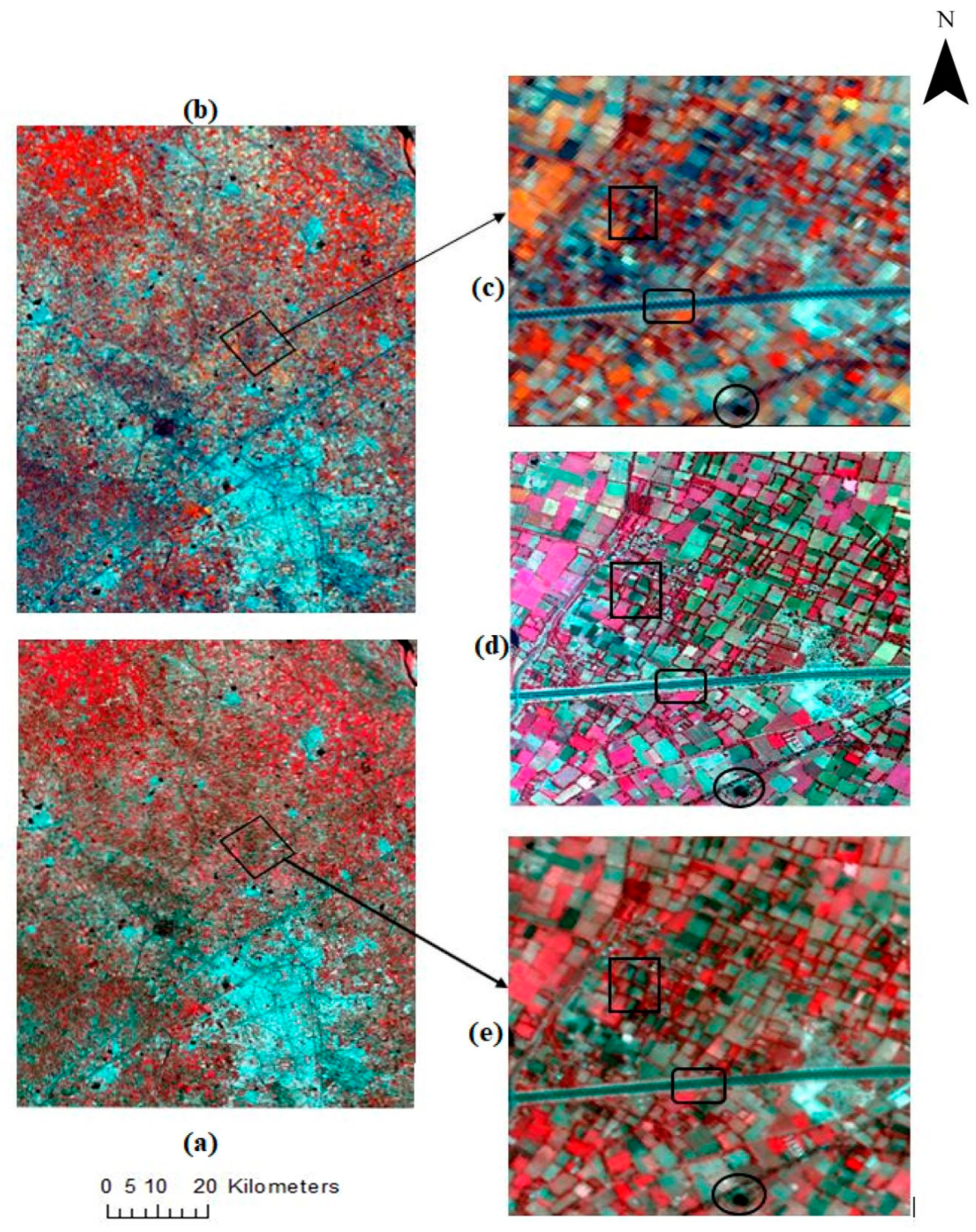
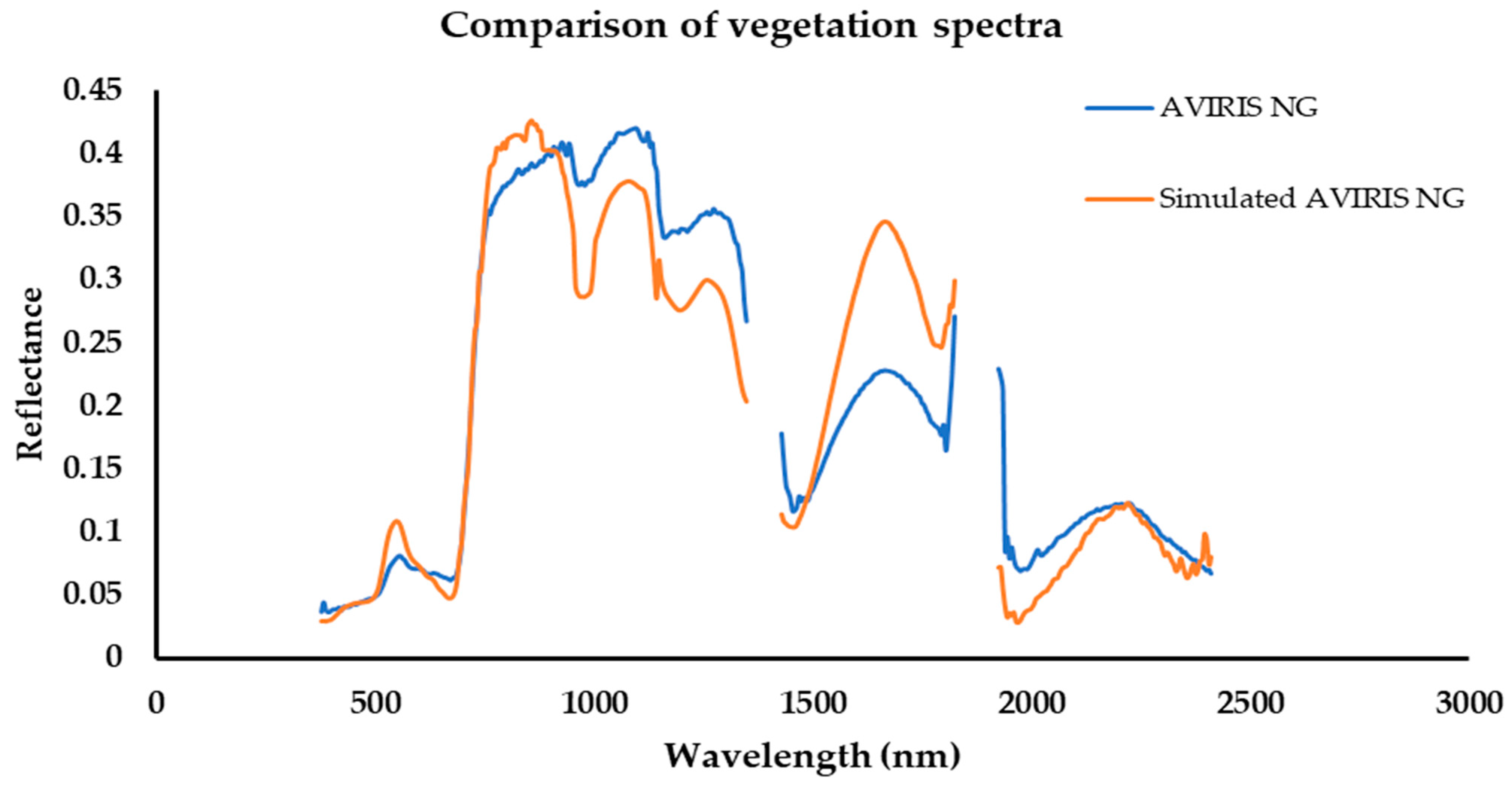
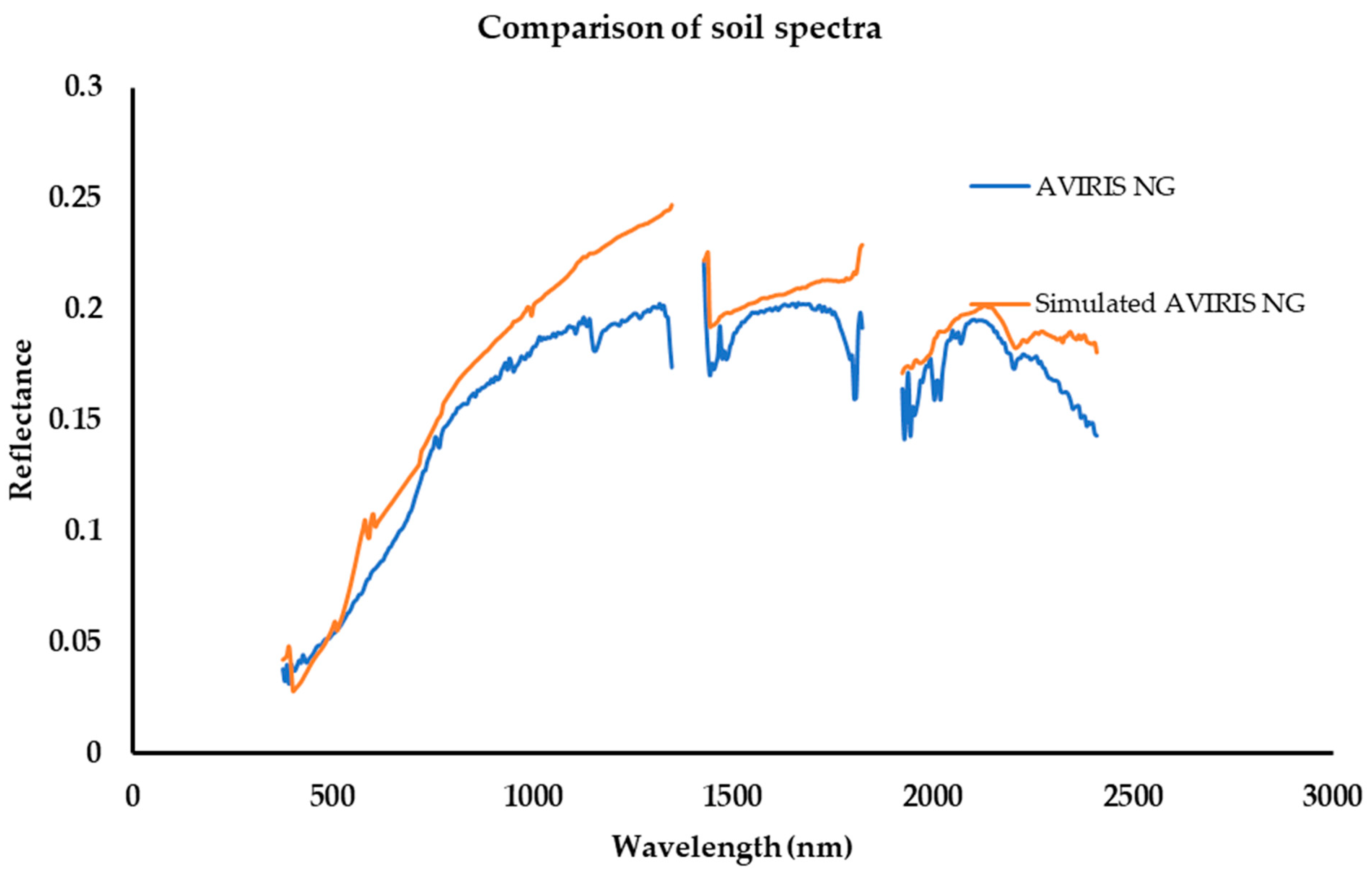
3.1. Simulation of AVIRIS-NG Imagery

In the present work, synthetic AVIRIS-NG imagery was generated using Sentinel-2 (multispectral imagery) and UPDM (a spectral unmixing method). Some of the noisy bands for the simulated and AVIRIS-NG were removed, i.e., bands from 1353.55–1423.67 nm, 1829.36–1919.53 nm, and 2415.38–2500.54 nm. Figure 1 shows the Sentinel-2 imagery and its corresponding simulated HS image, where a small portion from both the images is clipped out and compared with original AVIRIS-NG imagery. The red, green, and blue (RGB) band combination shown in the figure was bands 8, 4, and 3 for Sentinel-2 and bands 97, 56, and 36 for the simulated and AVIRIS-NG imagery. It is clear from the figure that the simulated image has more detailed information in addition to the richness expected in spectral resolution compared to the Sentinel-2 image, and it was quite close to the original AVIRIS-NG imagery. In order to further investigate the simulated imagery, Figure 3 and Figure 4 show the spectral comparison for vegetation, where it is evident that the simulated image showed a similar pattern from the blue to red edge (396.89–752.51 nm) region and from the SWIR to far-IR (1929.55–2405.37 nm) region. In the case of soil, regions 376.86–807.60 nm and 1924.54–2235.08 nm showed the best similarity with the original image. It is clear that the simulated imagery and AVIRIS-NG imagery have very good spectral signature similarity, and this property of simulated imagery could be further scrutinized for the vegetation parameter retrieval. Under close inspection, it can be seen that the simulated imagery has more clarity, and classes could be differentiated clearly as compared to Sentinel-2 image. To justify this, a few of the regions are marked in Figure 1. The squared region shows the ‘vegetation’ area, the rounded square area covers the ‘road’, and the circled portion shows the ‘water bodies’ in the clipped images of Sentinel-2, AVIRIS-NG, and simulated AVIRIS-NG. It is evident from the figure that the simulated image had clarity in spectral resolution as compared to the Sentinel-2 image. However, it is obvious that these classes were most easily identifiable in AVIRIS-NG. Thus, it is clear that the simulated image has a high degree of resemblance in characteristics compared to the original HS image.

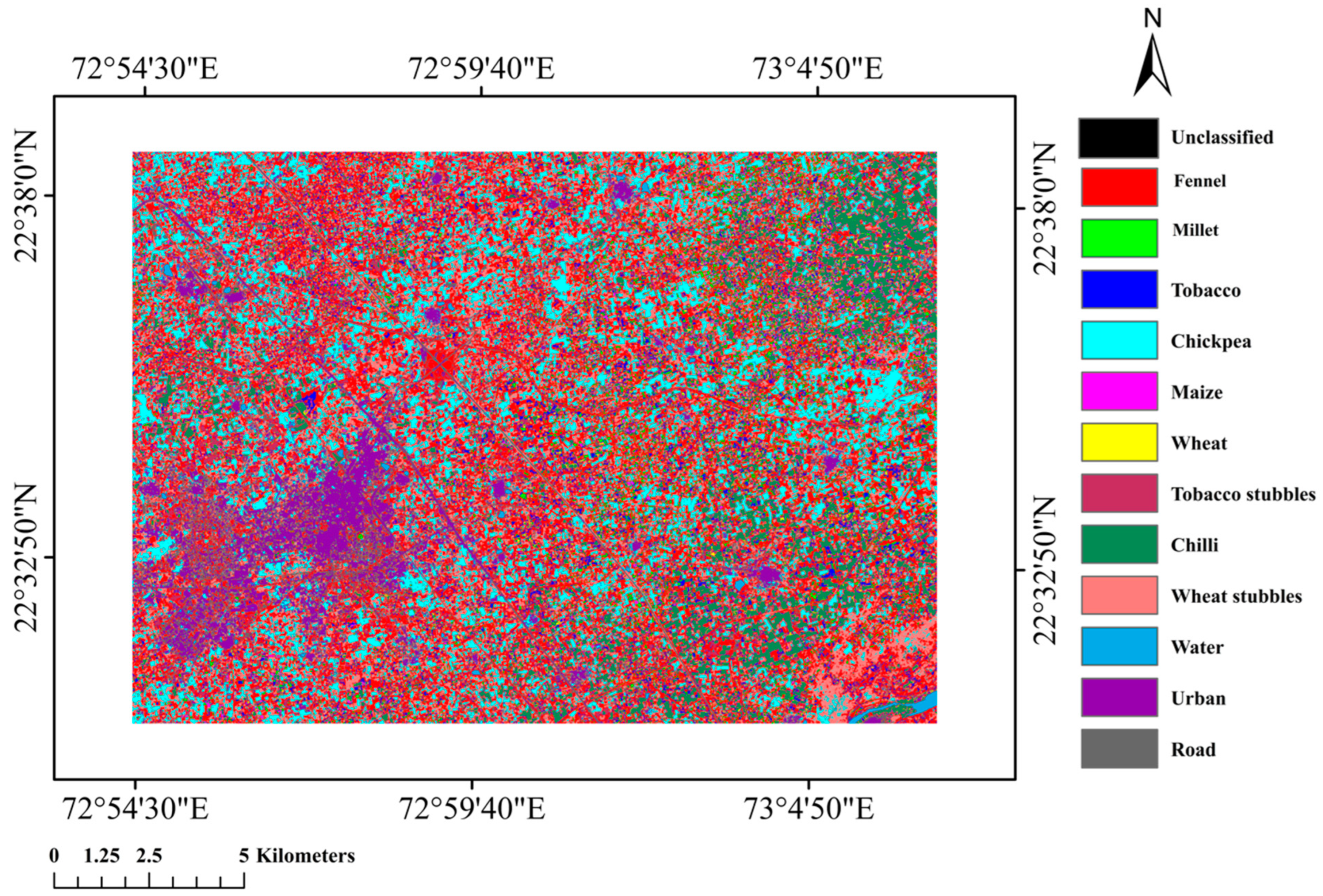
3.2. Classification of Simulated Image

During sampling, for the agricultural area, the region identified, i.e., the name of crops, was also noted. Furthermore, since the study area included urban, water bodies, and soil in addition to crops, a total of 12 classes were identified and given to the classifier. In total, 12 classes were identified using the SAM classifier in the simulated region, i.e., fennel (Foeniculum vulgare), millet (Pennisetum glaucum), tobacco (Nicotiana tabacum), chickpea (Cicer arietinum), maize (Zea mays), wheat (Triticum), tobacco stubbles, chili (Capsicum frutescens), and wheat stubbles, as well as urban, water, and road areas. Pure pixels were utilized to classify the image, and an independent set of ground datasets were used to validate the classified image. As endmembers to categorize different species and classes for the categorization, the spectral profiles from the sample sites were used. The performance of the classifier was evaluated using the overall accuracy (OA), kappa coefficient, precision, recall, and F1-score, as presented in Table 1. The overall accuracy came out to 87.40% with a kappa coefficient of 0.85.
Precision and recall are two critical model assessment measures. While precision is the proportion of relevant outcomes, recall is the percentage of total relevant results properly categorized by the algorithm. There is a simpler measure that considers both precision and recall, called the F1-score, which is just the harmonic mean of accuracy and recall. A higher value of this score indicates a better model, with a maximum attainable score of 1 or 100%.
Mathematically, the F1-score is calculated as follows:
F 1 = 2 × P r e c i s i o n × R e c a l l P r e c i s i o n + R e c a l l .
The user and producer accuracies for each class are shown in Table 2. It is evident that the ‘urban’ class has the highest user accuracy, whereas ‘fennel’ and ‘water’ have the highest producer accuracy.
An ROC curve is a binary classification problem assessment measure. It is a probability curve that separates ‘signal’ from ‘noise’. The AUC is a measure of a classifier’s ability to discriminate between classes and is used to summarize the ROC curve. An ROC curve was plotted for the classifier to show its performance, and the AUC was further calculated. A greater AUC indicates a better ability of the model in differentiating between positive and negative classes. When AUC = 1, the classifier works best to distinguish amongst classes; a value > 0.5 shows that the model performs well in classification. For the SAM classifier applied for each class, we obtained values > 0.9, as shown in Figure 6.

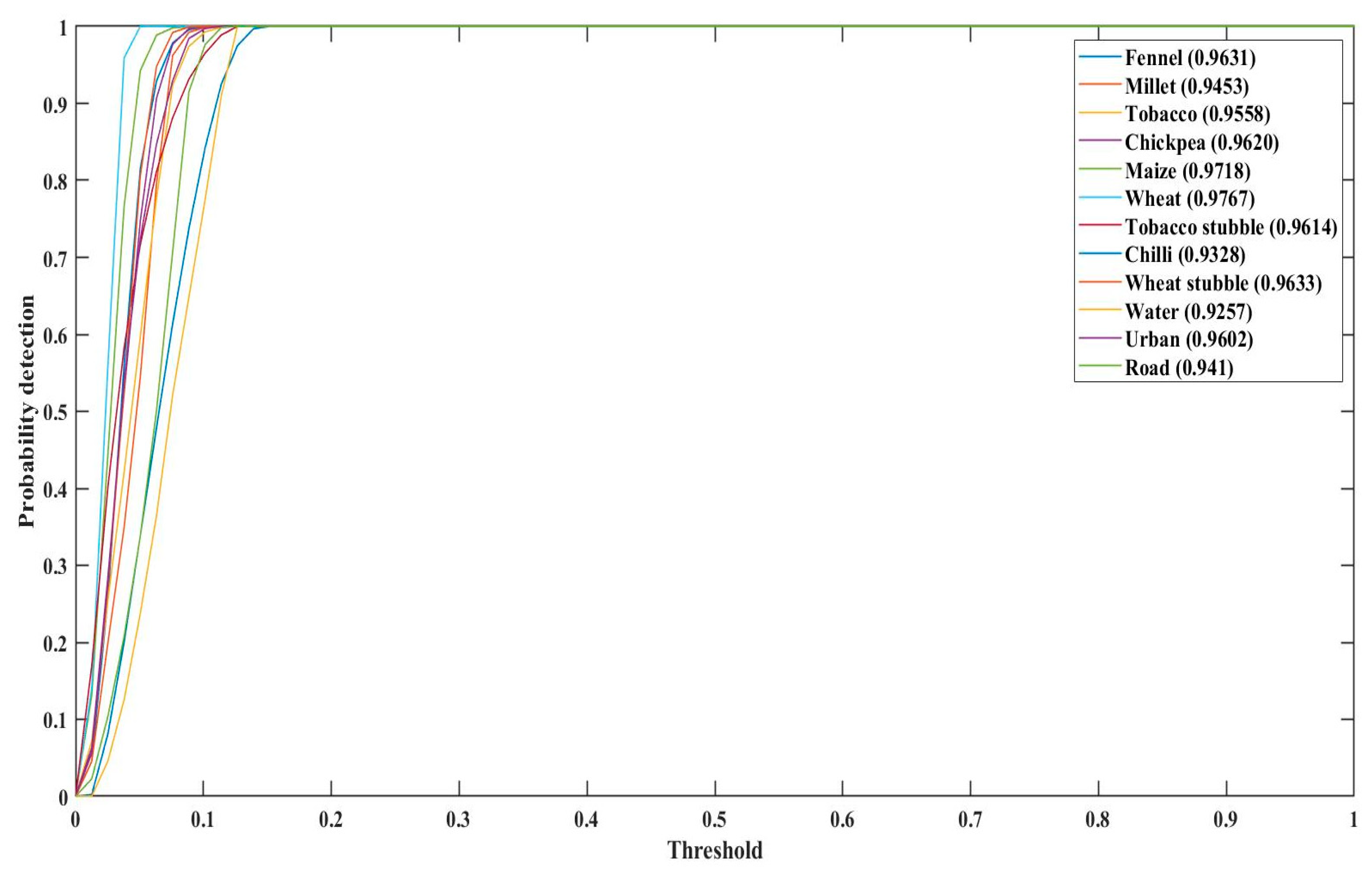
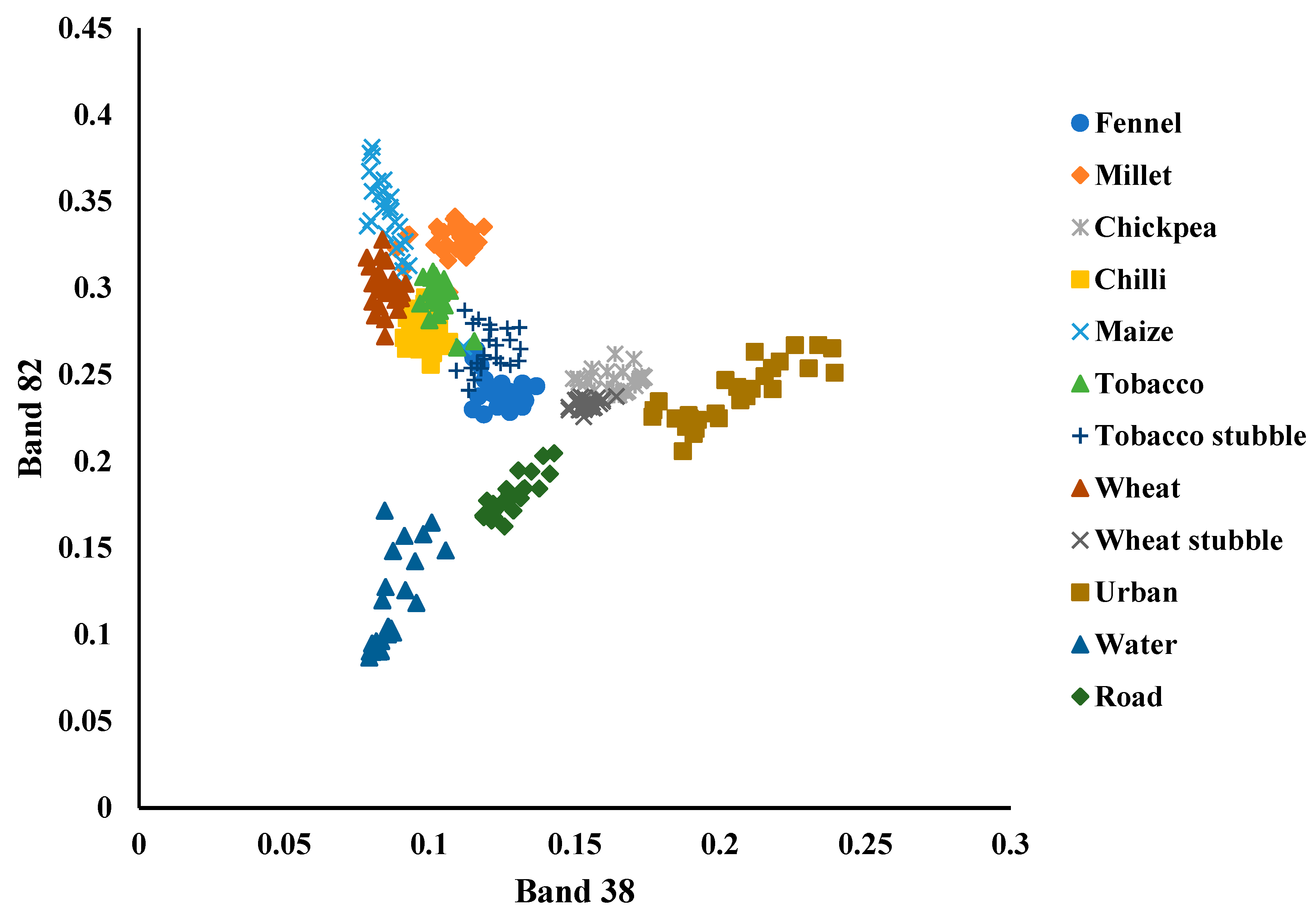
3.3. Class Separability Analysis
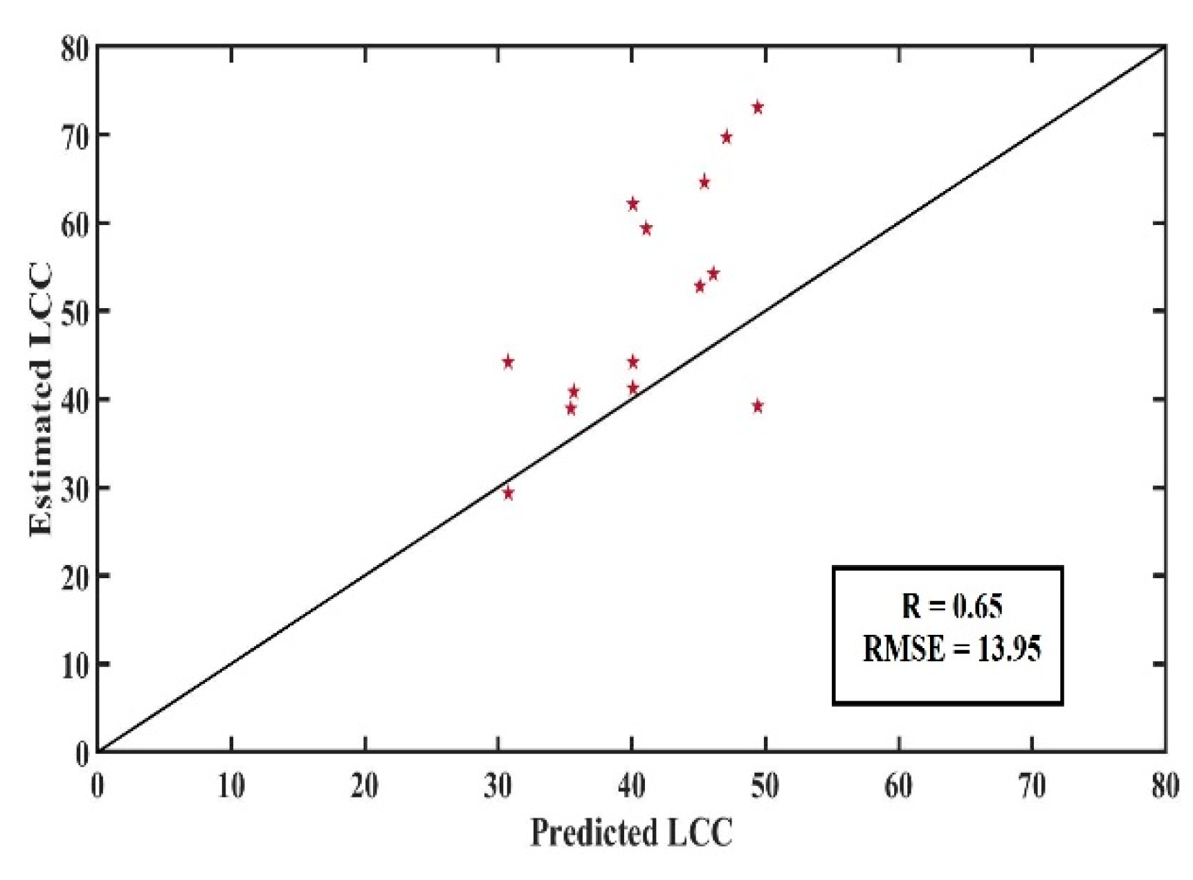
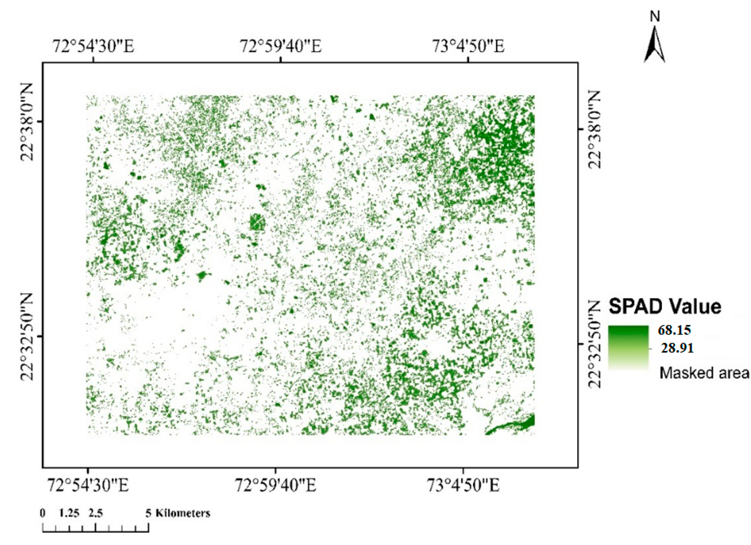
It is critical from the standpoint of computing cost and complexity that items of distinct classes be distinguished using specific metrics. The idea of class separability (CS) is one such statistic. The class separability plot was created utilizing pixel values between the two bands to evaluate any mixed pixel effects, as shown in Figure 7. CS was plotted for two bands, band 38 vs. band 82, chosen randomly. The plot shows that the ‘urban’, ‘water’, and ‘road’ classes were well separated. Moreover, classes of different vegetation were fairly separated with a few overlapping pixels amongst them.

3.4. LCC Retrieval

In order to estimate the LCC from the simulated HS imagery, the vegetation index CCI10, developed by Singh et al., was used for AVIRIS-NG imagery. CCI10 calculates the normalized ratio of bands 416 nm in the blue region and 1934 nm in the NIR region, and it was found to be the best model for the estimation of LCC in the vegetation area for the site. The estimated values for the LCC values for the entire area for simulated imagery were found in the range of 28.91 to 68.15 of SPAD values. These values were validated with the in-situ chlorophyll data, yielding R = 0.65, with RMSE value = 13.95. Figure 8 shows the chlorophyll map, and Figure 9 is the scatter plot for the comparison between estimated LCC and in situ LCC values. A chlorophyll map was generated for the simulated image of the entire area, using VI (Equation (11)) and the model (Equation (12)). In the chlorophyll map, areas with certain values in the lower and upper bounds were masked such that it showed values for the vegetation part only. The model was generated for the AVIRIS-NG campaign conducted at the same site for the year 2016 (Figure 8 and Figure 9).

4. Discussion

The presented work showed the efficiency of simulated hyperspectral imagery (AVIRIS-NG) for the retrieval of LCC. For the simulation of imagery, many endmember combinations were investigated to get the best possible results: vegetation–soil (VS), vegetation–soil–concrete (VSC), vegetation–soil–asphalt (VSA), and vegetation–soil–concrete–asphalt (VSCA). For VS and VSCA, we found poor results, whereas, for VSA and VSC, we got fair results, among which VSC gave the best estimation for the study site. Accordingly, it can be inferred that this model worked best with only three classes; thus, when using UPDM to generate imagery, only three distinct classes should be taken for calculation. From the simulated results, it is clear that there was higher similarity in the visible to red-edge region and far-SWIR region, whereas the model usually overestimated in the SWIR region for vegetation. However, in the case of soil, the model worked acceptably for almost the entire spectrum. Therefore, it can be deduced that this method may also work well for soil science studies. According to the findings of Zhang et al. [21] with respect to differences between simulated and original AVIRIS-NG spectra, they were much less for the visible to mid-infrared (<1000 nm) region, while some differences were seen beyond that. These differences could be due to the spatial resolution, since Sentinel-2 has 20 m spatial resolution in the SWIR band that we resampled to 10 m. The simulated imagery was more detailed than the Sentinel-2 imagery, and the generated hyperspectral data looked similar to the AVIRIS-NG data, with fine spatial features retained. Overall, the simulated hyperspectral imaging outperformed Sentinel-2 images in terms of spectral resolution. Classification was also performed on the simulated image, and it showed good accuracy, with classes tobacco, chickpea, maize, wheat, wheat stubbles, and urban having a user accuracy above 90%, whereas water had the lowest user accuracy value. For UPDM, three endmembers were used to simulate the image. Since there were 12 classes including different species of crops, urban areas, water bodies, roads, and buildings present in the study area, classification was run on the simulated image to check if the UPDM-generated image could effectively identify different classes.
In previous studies performed on the classification of simulated images via UPDM, Badola et al. [30] found that the classifier performed best on the AVIRIS-NG image with an accuracy of 94.6%, followed by simulated imagery (89%) and Sentinel-2 imagery (77.8%) for forestry area. They also assessed the effects of different reflectance values on classification accuracy, finding that, for up to a 25% difference in reflectance values, there was very low impact on classification accuracy. Liu et al. [5] also attempted classifying a simulated image (ALI multispectral to EO-1 hyperion data), and they found overall accuracies of 87.6% and 86.8% for simulated data and ALI data, respectively. Jyoti et al. [31] performed mangrove classification on AVIRIS-NG imagery using a support vector machine (SVM), and they found an accuracy of 87.61%, whereas Shahbaz et al. [32] performed vegetation species identification using SVM and ANN for an AVIRIS-NG image and found an accuracy of 86.75% and 86.45%. In view of the studies shown, the AVIRIS-NG simulated in this study showed very comparable results for classification purposes. The classification accuracy obtained for simulated AVIRIS-NG was very similar to the classification accuracy of the original AVIRIS-NG image; therefore, UPDM works well for the simulation of hyperspectral image.
In the CS analysis, performed on the classified image, it was found that almost every vegetation species had a few overlapping pixels, and, albeit fairly separated, all of the vegetation classes were near to each other. This could be explained by the fact that, while providing endmembers to the UPDM algorithm, one type of vegetation spectrum was used in the calculation; hence, the base spectrum for each species was the same.
The LCC retrieval was performed using linear regression from the CCI10 model, and the accuracy of the model can be further increased if nonlinear regression is implemented. Furthermore, use of the radiative transfer model can also be explored. Until now, no study has investigated the usefulness of simulated AVIRIS-NG imagery for the estimation of vegetation parameters. Therefore, in order to extend the application of the data simulation from UPDM to precision agriculture, a chlorophyll map was generated for the entire area. LCC estimated using the CCI10 model from the spectra generated was compared with the in-situ data, revealing acceptable results. It was found that spectra in visible, red-edge, SWIR, and far-IR regions showed good correlation with the original AVIRIS-NG bands. The regions near 1900 nm and 416 nm showed similar trends to the original image, indicating a good correlation with LCC in terms of the CCI10 VI model.

5. Conclusions

In the presented study, hyperspectral imagery for AVIRIS-NG was simulated by utilizing a spectral reconstruction approach (UPDM) and multispectral imagery (Sentinel-2). The generated image was further evaluated with statistical analysis and visually interpreted. In order to explore the usability of the generated model in terms of vegetation biochemical parameter retrieval, it was applied to calculate the leaf chlorophyll content for different vegetation species. A chlorophyll map for the region was generated to show the variation in LCC of different vegetation under different stages, and this was validated for some points by LCC taken during data sampling. Singh et al. generated different models for the estimation of LCC for the same region using AVIRIS-NG imagery, and the best model (R = 0.706) for the site was chosen to retrieve LCC for simulated HS imagery. It was found that the simulated imagery gave quite agreeable (R = 0.65) LCC values with respect to in situ data. In conclusion, this free-of-cost HS imagery simulated using UPDM and MS imagery can be used further in the agriculture community for the retrieval of vegetation parameters.

Author Contributions

Conceptualization, B.V. and A.B.; methodology, B.V. and A.B.; software, B.V.; validation, B.V. and P.S.; formal analysis, B.V.; investigation, B.V.; resources, P.K.S.; data curation, P.K.S. and P.S.; writing—original draft preparation, B.V.; writing—review and editing, B.V., R.P. and A.B.; visualization, J.S.; supervision, R.P. and P.K.S. All authors have read and agreed to the published version of the manuscript.

Funding

This research received funding from Space Application Center, ISRO under the Grant number P-32/20.

Data Availability Statement

The AVIRIS-NG data used in this study can be made available upon request. The Sentinel-2 dataset is freely available through the Copernicus website.

Acknowledgments

The authors would like to thank SAC-ISRO for providing AVIRIS-NG imagery. The authors would like to extend their gratitude to MHRD (Government of India) and the Indian Institute of Technology (BHU) for providing financial assistance.

Conflicts of Interest

The authors declare no conflict of interest.

References

  1. Varshney, P.K.; Arora, M.K. Advanced Image Processing Techniques for Remotely Sensed Hyperspectral Data; Springer Science & Business Media: Berlin/Heidelberg, Germany, 2004. [Google Scholar]
  2. Kavzoglu, T. Simulating Landsat ETM+ imagery using DAIS 7915 hyperspectral scanner data. Int. J. Remote Sens. 2004, 25, 5049–5067. [Google Scholar] [CrossRef]
  3. Justice, C.O.; Markham, B.L.; Townshend, J.R.G.; Kennard, R.L. Spatial degradation of satellite data. Int. J. Remote Sens. 1989, 10, 1539–1561. [Google Scholar] [CrossRef]
  4. Li, J.; Sensing, R. Spatial quality evaluation of fusion of different resolution images. Int. Arch. Photogramm. Remote Sens. 2000, 33, 339–346. [Google Scholar]
  5. Liu, B.; Zhang, L.; Zhang, X.; Zhang, B.; Tong, Q.J.S. Simulation of EO-1 hyperion data from ALI multispectral data based on the spectral reconstruction approach. Sensors 2009, 9, 3090–3108. [Google Scholar] [CrossRef]
  6. Houborg, R.; Anderson, M.; Daughtry, C. Utility of an image-based canopy reflectance modeling tool for remote estimation of LAI and leaf chlorophyll content at the field scale. Remote Sens. Environ. 2009, 113, 259–274. [Google Scholar] [CrossRef]
  7. Zarco-Tejada, P.J.; Miller, J.R.; Morales, A.; Berjón, A.; Agüera, J. Hyperspectral indices and model simulation for chlorophyll estimation in open-canopy tree crops. Remote Sens. Environ. 2004, 90, 463–476. [Google Scholar] [CrossRef]
  8. Singh, P.; Pandey, P.C.; Petropoulos, G.P.; Pavlides, A.; Srivastava, P.K.; Koutsias, N.; Deng, K.A.K.; Bao, Y. Hyperspectral remote sensing in precision agriculture: Present status, challenges, and future trends. In Hyperspectral Remote Sensing; Elsevier: Amsterdam, The Netherlands, 2020; pp. 121–146. [Google Scholar]
  9. Curran, P.J.; Kupiec, J.A.; Smith, G.M. Remote sensing the biochemical composition of a slash pine canopy. IEEE Trans. Geosci. Remote Sens. 1997, 35, 415–420. [Google Scholar] [CrossRef]
  10. Matson, P.; Johnson, L.; Billow, C.; Miller, J.; Pu, R. Seasonal patterns and remote spectral estimation of canopy chemistry across the Oregon transect. Ecol. Appl. 1994, 4, 280–298. [Google Scholar] [CrossRef]
  11. Zarco-tejada, P.J.; Miller, J.R. Land cover mapping at BOREAS using red edge spectral parameters from CASI imagery. J. Geophys. Res. Atmos. 1999, 104, 27921–27933. [Google Scholar] [CrossRef]
  12. Johnson, L.F.; Hlavka, C.A.; Peterson, D.L. Multivariate analysis of AVIRIS data for canopy biochemical estimation along the Oregon transect. Remote Sens. Environ. 1994, 47, 216–230. [Google Scholar] [CrossRef]
  13. Moulin, S. Impacts of model parameter uncertainties on crop reflectance estimates: A regional case study on wheat. Int. J. Remote Sens. 1999, 20, 213–218. [Google Scholar] [CrossRef]
  14. Demarez, V. Seasonal variation of leaf chlorophyll content of a temperate forest. Inversion of the PROSPECT model. Int. J. Remote Sens. 1999, 20, 879–894. [Google Scholar] [CrossRef]
  15. Ganapol, B.D.; Johnson, L.F.; Hammer, P.D.; Hlavka, C.A.; Peterson, D.L. LEAFMOD: A new within-leaf radiative transfer model. Remote Sens. Environ. 1998, 63, 182–193. [Google Scholar] [CrossRef]
  16. Jacquemoud, S.; Baret, F. PROSPECT: A model of leaf optical properties spectra. Remote Sens. Environ. 1990, 34, 75–91. [Google Scholar] [CrossRef]
  17. Renzullo, L.J.; Blanchfield, A.L.; Guillermin, R.; Powell, K.S.; Held, A.A. Comparison of PROSPECT and HPLC estimates of leaf chlorophyll contents in a grapevine stress study. Int. J. Remote Sens. 2006, 27, 817–823. [Google Scholar] [CrossRef]
  18. Verma, B.; Prasad, R.; Srivastava, P.K.; Yadav, S.A.; Singh, P.; Singh, R.K. Investigation of optimal vegetation indices for retrieval of leaf chlorophyll and leaf area index using enhanced learning algorithms. Comput. Electron. Agric. 2022, 192, 106581. [Google Scholar] [CrossRef]
  19. Verrelst, J.; Muñoz, J.; Alonso, L.; Delegido, J.; Rivera, J.P.; Camps-Valls, G.; Moreno, J. Machine learning regression algorithms for biophysical parameter retrieval: Opportunities for Sentinel-2 and-3. Remote Sens. Environ. 2012, 118, 127–139. [Google Scholar] [CrossRef]
  20. Li, F.; Mistele, B.; Hu, Y.; Chen, X.; Schmidhalter, U. Reflectance estimation of canopy nitrogen content in winter wheat using optimised hyperspectral spectral indices and partial least squares regression. Eur. J. Agron. 2014, 52, 198–209. [Google Scholar] [CrossRef]
  21. Zhang, L.; Furumi, S.; Muramatsu, K.; Fujiwara, N.; Daigo, M.; Zhang, L. Sensor-Independent Analysis Method for Hyper-Multispectral Data Based on the Pattern Decomposition Method. Int. J. Remote Sens. 2006, 27, 4899–4910. [Google Scholar] [CrossRef]
  22. Hirapara, J.; Singh, P.; Singh, M.; Patel, C.D. Analysis of rainfall characteristics for crop planning in north and south Saurashtra region of Gujarat. J. Agric. Eng. 2020, 57, 162–171. [Google Scholar]
  23. Srivastava, P.K.; Malhi, R.K.M.; Pandey, P.C.; Anand, A.; Singh, P.; Pandey, M.K.; Gupta, A. Revisiting hyperspectral remote sensing: Origin, processing, applications and way forward. In Hyperspectral Remote Sensing; Elsevier: Amsterdam, The Netherlands, 2020; pp. 3–21. [Google Scholar]
  24. Bhattacharya, B.; Green, R.O.; Rao, S.; Saxena, M.; Sharma, S.; Kumar, K.A.; Srinivasulu, P.; Sharma, S.; Dhar, D.; Bandyopadhyay, S.; et al. An overview of AVIRIS-NG airborne hyperspectral science campaign over India. Curr. Sci. 2019, 116, 1082–1088. [Google Scholar] [CrossRef]
  25. Chapman, J.W.; Thompson, D.R.; Helmlinger, M.C.; Bue, B.D.; Green, R.O.; Eastwood, M.L.; Geier, S.; Olson-Duvall, W.; Lundeen, S.R. Spectral and radiometric calibration of the next generation airborne visible infrared spectrometer (AVIRIS-NG). Remote Sens. 2019, 11, 2129. [Google Scholar] [CrossRef] [Green Version]
  26. Anand, A.; Malhi, R.K.M.; Srivastava, P.K.; Singh, P.; Mudaliar, A.N.; Petropoulos, G.P.; Kiran, G.S. Optimal band characterization in reformation of hyperspectral indices for species diversity estimation. Phys. Chem. Earth 2021, 126, 103040. [Google Scholar] [CrossRef]
  27. Pandey, P.C.; Pandey, M.K.; Gupta, A.; Singh, P.; Srivastava, P.K. Spectroradiometry: Types, data collection, and processing. In Advances in Remote Sensing for Natural Resource Monitoring; Pandey, P.C., Sharma, L.K., Eds.; Wiley: Hoboken, NJ, USA, 2021; pp. 9–27. [Google Scholar]
  28. Uddling, J.; Gelang-Alfredsson, J.; Piikki, K.; Pleijel, H. Evaluating the relationship between leaf chlorophyll concentration and SPAD-502 chlorophyll meter readings. Photosynth. Res. 2007, 91, 37–46. [Google Scholar] [CrossRef]
  29. Singh, P.; Srivastava, P.K.; Malhi, R.K.M.; Chaudhary, S.K.; Verrelst, J.; Bhattacharya, B.K.; Raghubanshi, A.S. Denoising AVIRIS-NG data for generation of new chlorophyll indices. IEEE Sens. J. 2020, 21, 6982–6989. [Google Scholar] [CrossRef]
  30. Badola, A.; Panda, S.K.; Roberts, D.A.; Waigl, C.F.; Bhatt, U.S.; Smith, C.W.; Jandt, R.R. Hyperspectral Data Simulation (Sentinel-2 to AVIRIS-NG) for Improved Wildfire Fuel Mapping, Boreal Alaska. Remote Sens. 2021, 13, 1693. [Google Scholar] [CrossRef]
  31. Hati, J.P.; Samanta, S.; Chaube, N.R.; Misra, A.; Giri, S.; Pramanick, N.; Gupta, K.; Majumdar, S.D.; Chanda, A.; Mukhopadhyay, A.; et al. Mangrove classification using airborne hyperspectral AVIRIS-NG and comparing with other spaceborne hyperspectral and multispectral data. Egypt. J. Remote Sens. Space Sci. 2021, 24, 273–281. [Google Scholar]
  32. Ahmad, S.; Pandey, A.C.; Kumar, A.; Lele, N.V. Potential of hyperspectral AVIRIS-NG data for vegetation characterization, species spectral separability, and mapping. Appl. Geomat. 2021, 13, 361–372. [Google Scholar] [CrossRef]
Figure 1. (a) Simulated AVIRIS-NG (bands 97, 56, and 36); (b) Sentinel-2 imagery (bands 8, 4, and 3); (c) clipped area for Sentinel-2 imagery; (d) AVIRIS-NG imagery (bands 97, 56, and 36); (e) clipped area for simulated AVIRIS-NG imagery.
Remotesensing 14 03560 g001
Figure 2. (a) Spectral response function for the sensors of AVIRIS-NG (for the first 90 bands); (b) spectral response function for the sensors of Sentinel-2.
Remotesensing 14 03560 g002
Figure 3. Comparison of vegetation spectra for AVIRIS-NG and simulated AVIRIS-NG.
Remotesensing 14 03560 g003
Figure 4. Comparison of soil spectra for AVIRIS-NG and simulated AVIRIS-NG.
Remotesensing 14 03560 g004
Figure 5. Classification on the simulated image.
Remotesensing 14 03560 g005
Figure 6. ROC curve for the classification with AUC values.
Remotesensing 14 03560 g006
Figure 7. Class separability chart.
Remotesensing 14 03560 g007
Figure 8. Chlorophyll map for the simulated AVIRIS-NG.
Remotesensing 14 03560 g008
Figure 9. Comparison of LCC estimated with in situ data.
Remotesensing 14 03560 g009
Table 1. Performance assessment of the classifier.
Overall AccuracyPrecisionRecallF1-ScoreKappa Coefficient
87.40%85.63%83.29%84.47%0.85
Table 2. Producer and user accuracy of each class for the classified image.
ClassesProducer Accuracy
(%)
User Accuracy
(%)
Fennel10078.4
Millets74.2289.95
Tobacco72.5195.63
Chickpea98.8594.44
Maize66.4190.23
Wheat42.6898
Tobacco stubbles97.7273.94
Chili99.8484.86
Wheat stubbles86.592.06
Water10042.8
Urban88.1298.24
Road72.6589.17
Unclassified0.07100
Publisher’s Note: MDPI stays neutral with regard to jurisdictional claims in published maps and institutional affiliations.

