Cross-Comparison of Individual Tree Detection Methods Using Low and High Pulse Density Airborne Laser Scanning Data

Abstract

Numerous individual tree detection (ITD) methods have been developed for use with airborne laser scanning (ALS) data to provide tree-scale forest inventories across large spatial extents. Despite the growing number of methods, relatively few have been comparatively assessed using a single benchmark forest inventory validation dataset, limiting their operational application. In this study, we assessed seven ITD methods, representing three common approaches (point-cloud-based, raster-based, hybrid), across coniferous forest stands with diverse structure and composition to understand how ITD and height measurement accuracy vary with method, input parameters and data, and stand density. There was little variability in accuracy between the ITD methods where the average F-score and standard deviation (±SD) were 0.47 ± 0.03 using a lower pulse density ALS dataset with an average of 8 pulses per square meter (ppm²) and 0.50 ± 0.02 using a higher pulse density ALS dataset with an average of 22 ppm². Using higher ALS pulse density data produced higher ITD accuracies (F-score increase of 10–13%) in some of the methods versus more modest gains in other methods (F-score increase of 1–3%). Omission errors were strongly related with stand density and largely consisted of suppressed trees underneath the dominant canopy. Simple canopy height model (CHM)-based methods that utilized fixed-size local maximum filters had the lowest omission errors for trees across all canopy positions. ITD accuracy had large intra-method variation depending on input parameters; however, the highest accuracies were obtained when parameters such as search window size and spacing thresholds were equal to or less than the average crown diameter of trees in the study area. All ITD methods produced height measurements for the detected trees that had low RMSE (<1.1 m) and bias (<0.5 m). Overall, the results from this study may help guide end-users with ITD method application and highlight future ITD method improvements.

1. Introduction

Accurate forest inventories are necessary for sustainable forest management and supply chain planning. For more than a century, manually collected subsampling of tree conditions across a landscape has driven forest inventory. These conventional methods are time- and accuracy-limited [1] and are often cost-prohibitive to execute at large scales [2]. Numerous methods utilizing airborne scanning light detection and ranging (LiDAR), commonly referred to as airborne laser scanning (ALS), have been developed to predict stand-level forest inventories and imputations of population-level summaries, and detect individual tree locations at various spatial extents [3,4,5,6]. The segmentation of single-trees from ALS is often referred to as individual tree detection (ITD) and multiple methods have been developed and broadly considered as potential tools for providing near-census forest inventories [7,8,9], improving growth and yield modeling [10,11,12], monitoring tree-scale growth and mortality [13], and optimizing harvest planning and operations [14]. A limited number of studies have assessed different ITD method approaches using a single benchmark dataset [15,16,17,18]. The study by [17] is notable as it evaluated eight ITD methods using high-density (5–121 ppm²) ALS data in the Alps. However, cross-comparison of ITD methods to benchmark datasets associated with different forest structures remains relevant, especially given the rapid advances in ALS technology, computational power, and machine learning.

Individual tree detection methods using ALS data can generally be grouped into three major types based on what input data they use: point-cloud-based, raster-based, and hybrid approaches. Point-cloud-based approaches identify individual trees using a variety of methods that take advantage of tree crown shape and spacing (e.g., [19]) and vertical and horizontal return density changes in the ALS point cloud (e.g., [20]). Raster-based ITD methods rely on gridded data that provide summary information extracted from ALS point clouds, such as minimum and maximum height of all returns within a grid cell. Raster-based ITD methods typically use canopy height models (CHMs), which represent the normalized height of non-ground objects in each grid cell. Many ITD methods that use CHMs focus on techniques to find local maxima in the CHM, which are assumed to be treetops [21,22,23,24]. Hybrid ITD approaches utilize gridded point cloud data (e.g., CHMs) and information extracted from the original point cloud to identify individual trees. In some approaches, CHMs are used to initially identify trees/tree clusters and the point cloud is used to further separate those clusters into individuals [9,25].

Numerous ITD approaches have been proposed and discussed throughout the literature in both formal and informal reviews [3,23,26,27,28,29,30]; however, there are a limited number of method comparison and benchmark studies available and these have been predominantly focused on forests in Europe (e.g., [15,16,17,18,31]). Many of these comparison studies have employed data ≥10 years old and have not assessed data from contemporary ALS sensors. These prior studies found that regardless of ITD method, dominant trees (trees in dominant and codominant canopy-height positions) have higher detection rates than subdominant trees (trees in intermediate and suppressed canopy-height positions), owing to smaller trees being occluded by the dominant forest canopy [32,33]. Some benchmarking studies found that choice of method was the dominant factor of ITD accuracy [16], while others found that stand density and structure were more important [17,31]. Furthermore, ALS pulse density has been found to improve ITD accuracy in some studies [18,34] but not others [16], with discrepancies potentially resulting from the sensor model, acquisition flight parameters, and/or laser-scanning pattern [3,35].

While prior benchmarking has provided valuable comparison information on ITD approaches, uncertainties remain for forests within North America (e.g., [4]), partly as a result of advances in ALS technology and processing tools. In particular, there is an outstanding need for testing and comparing ITD methods in forests with high tree species diversity where crown shapes and structure vary significantly, like many forests found in North America. Additionally, the effects of input-parameter selection and methodology on the resulting accuracy are not well-understood. As different ITD methods become incorporated into freely available processing tools and software (e.g., LidR [36], rLiDAR [24], FUSION [37]), it is increasingly important to assess how the accuracy of these methods compare with commercial products that may not provide the user with detailed descriptions of the underlying methodologies (e.g., grey- or black-box methods) to help guide end-user decisions and application.

The need for accurate, timely, and cost-effective forest inventory information has continued to increase globally as end-users decide actions to meet objectives on forested landscapes, and developers identify improvements to ITD methods. Therefore, the objective of this study was to understand how ITD accuracy varies by method, input parameters, and pulse density of the input ALS data across coniferous forest stands with diverse stand structure and composition within the inter-mountain West, USA. Seven ITD methods, representing three common approaches (point-cloud-based, raster-based, and hybrid), were assessed for ITD and height measurement accuracy via comparison with a single benchmark forest inventory dataset in north-central Idaho, USA. All methods were tested using a lower pulse density ALS dataset with an average of 8 pulses per square meter (ppm²) and a higher pulse density ALS dataset with an average of 22 ppm², and accuracies were reported using a suite of standard metrics.

2. Materials and Methods

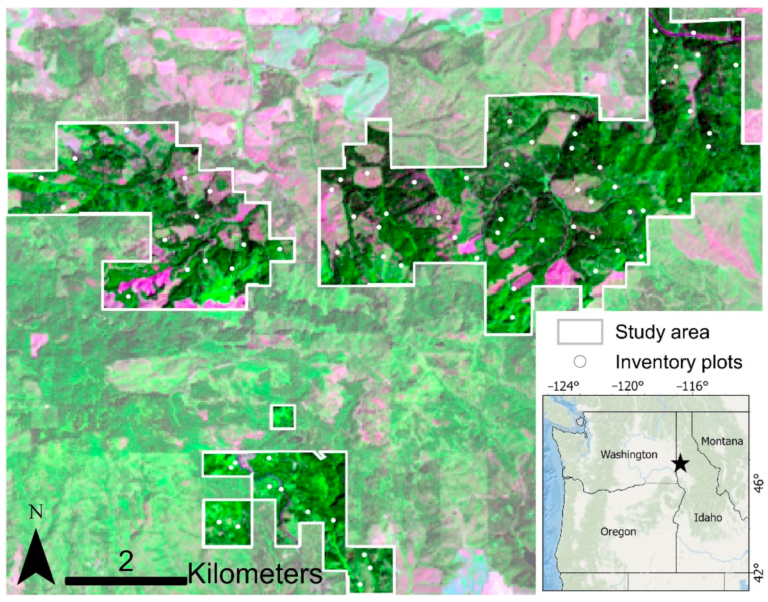
2.1. Study Area

This study was conducted in the University of Idaho Experimental Forest (UIEF), which is located on the Palouse Range in north-central Idaho, USA (Figure 1). The UIEF is a mixed-conifer temperate forest and dominant tree species include Pseudotsuga menziesii (Mirb.) Franco var. glauca (Beissn.) Franco (Douglas fir), Abies grandis (Douglas ex D. Don) Lindl. (grand fir), Thuja plicata Donn ex D. Don (western redcedar), and Larix occidentalis Nutt. (western larch). Other species within the study area include Pinus ponderosa C. Lawson var. scopulorum Engelm. (ponderosa pine), Pinus contorta Douglas ex Louden (lodgepole pine), Pinus monticola var. minima Lemmon (western white pine), and Picea engelmannii var. glabra Goodman (Engelmann spruce). The species within the study area have high crown shape and structure diversity ranging from narrow, pyramid-like crowns (e.g., Pseudotsuga menziesii, Larix occidentalis), to rounded cylindrical crowns (e.g., Pinus ponderosa, Pinus contorta), to irregularly shaped crowns (e.g., Thuja plicata). The UIEF has a diverse range of stand structures and composition (Figure 1) resulting from its multi-use management for timber, research, and education purposes. Prior studies have used this location to evaluate ITD and stand-level forest structural attributes due to the variability of stand structure and species (e.g., [4,23,38,39]).

2.2. ALS Data and Preprocessing

Two ALS datasets were used in this study. The first ALS dataset was acquired across the study area in the summer of 2018. These data were collected with a Teledyne Geospatial Optec Galaxy PRIME sensor (Teledyne Geospatial, Toronto, ON, Canada) mounted on a fixed-wing aircraft and collected under the guidance of the Teledyne Geospatial SwathTRAK™ software to achieve a 50% flight-line overlap with respect to the 60-degree sensor field-of-view. SwathTRAK™ software uses plane pitch, roll, and yaw for optimization of flight line efficiencies by varying the field-of-view to account for areas with highly variable terrain. Elevation of the aircraft varied between 3550 and 4200 m above ground level and flight lines alternated orientations while maintaining an average pulse density of 8 pulses per square meter. The average per-pulse return rate over forested areas was two. These ALS data were processed using GeoCue LP360 (GeoCue, Huntsville, AL, USA) and Terrasolid TerraScan software (Terrasolid, Helsinki, Finland) and returns were classified as bare earth and vegetation following the 2019 United States Geological Survey, 3D elevation program (3DEP) specification [40] before being delivered as 1000 m² tiles.

The second ALS dataset was acquired across the study area in the summer of 2021, using a RIEGL VQ-1560II sensor (RIEGL, Horn, Austria) mounted on a fixed-wing aircraft fitted with a gyro-stabilized mount. Elevation of the aircraft was maintained between 1700 and 1900 m above ground level and flight lines alternated orientations while maintaining a 55% flight-line overlap with respect to a 58-degree sensor field-of-view. The average pulse density was 22 pulses per square meter and the average per-pulse return rate over forested areas was four. These ALS data were preprocessed by the supplier to normalize laser intensity using the RIEGL RiPROCESS software, and returns were classified as bare earth, vegetation, water, buildings, and noise before being delivered as 500 m² tiles.

2.3. Field Validation Dataset

Sixty-seven 13 m radius forest inventory plots were established in the summer of 2020 following a stratified sampling design (Figure 1). The plot sampling strategy was designed to capture the variation in structure and composition across the study area and was guided by structural metrics derived from the ALS point clouds. All plots were precisely located using a Triumph-2 global navigation system (JAVAD, San Jose, CA, USA) and Samsung Galaxy tablet with a Rover pole. All trees > 1.5 m in height were stem-mapped using azimuth and distance from plot center using a Vertex Laser Geo 360 (Haglof, Sweden). In addition to location, each tree was measured for height, DBH, species, live/dead status, and canopy position (i.e., dominant, codominant, intermediate, and suppressed). Canopy position definitions were adapted from [41], where dominant trees receive light from 3–4 directions, codominant trees receive light from 1–2 directions, intermediate trees receive light mainly from the top, and suppressed trees are entirely shaded and underneath the stand canopy. Tree measurement summary statistics are presented in

Table 1. Tree measurement summary statistics for the validation inventory plots.

Metric	Minimum	Maximum	Median	Mean	SD
Tree Density (trees/ha)	18.8	1846.7	508.8	542.7	386.7
Basal Area (m2/ha)	0.4	111.6	31.3	31.9	23.0
DBH (cm)	5.1	137.2	19.1	23.2	14.6
Height (m)	6.1	40.9	14	15.9	7.6

.

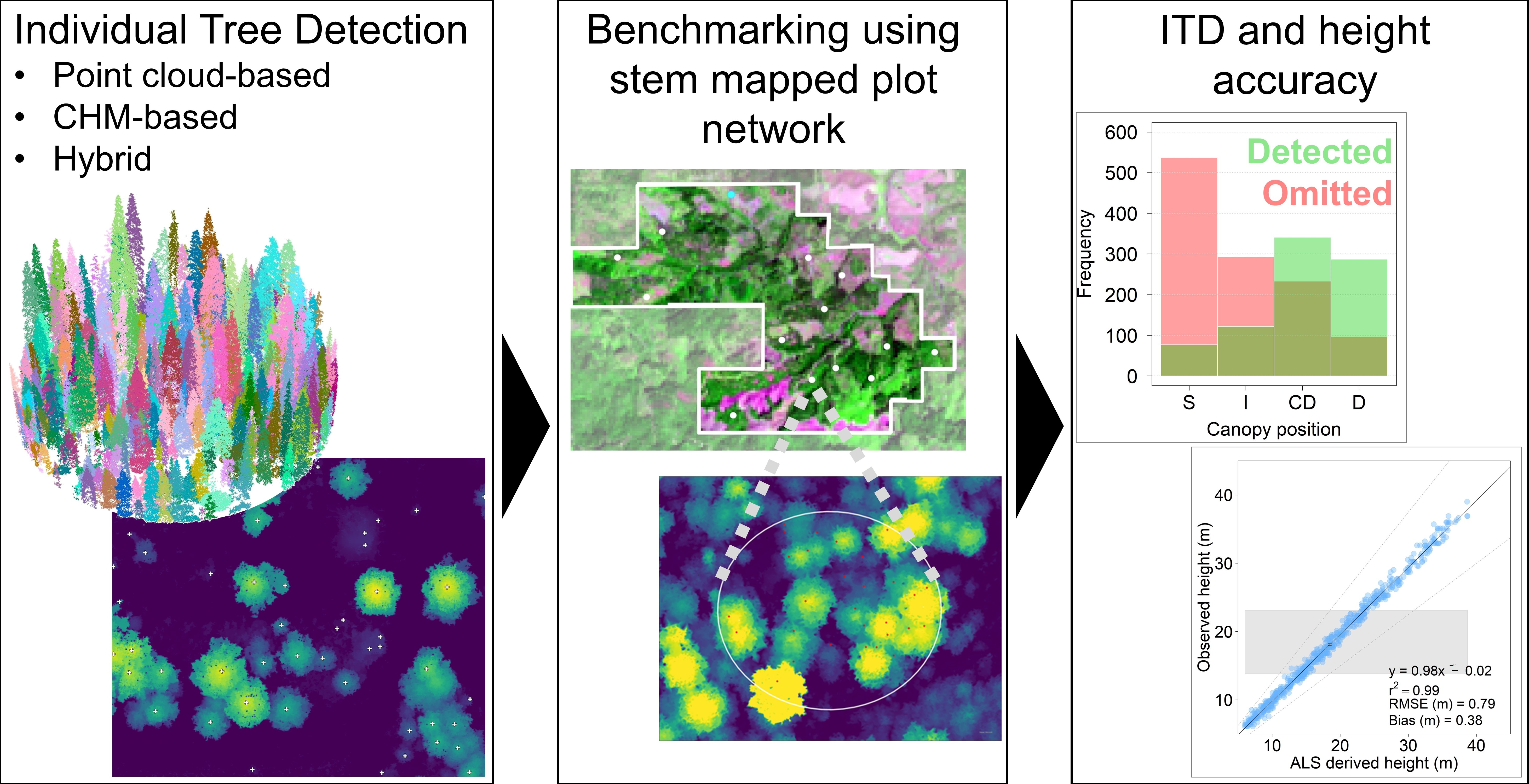
2.4. Individual Tree Detection Methods

Seven ITD methods, representing three common approaches (point-cloud-based, raster-based, hybrid), were assessed for individual tree detection and height measurement accuracy. Each method can produce widely varying results depending on the input data and parameters. To assess which parameter combinations were the most accurate, we tested each method using both ALS datasets and multiple parameter inputs. The following sections describe the input data and parameters used for each method approach and

Table 2. ITD method approaches tested in this study. CHM: canopy height model; SW: search window.

Method	ALS Pulse Density (ppm2)	Input Parameters	Total # of Method Approaches
ForestView®	8	Default CHM and point cloud metrics	1
	22	Default CHM and point cloud metrics	1
[19]	8	3 spacing thresholds	3
	22	3 spacing thresholds	3
lidR LMF	8	2 CHM resolutions, 3 SW sizes, 2 SW shapes	12
	22	3 CHM resolutions, 3 SW sizes, 2 SW shapes	18
rLiDAR LMF	8	2 CHM resolutions, 3 SW sizes, 1 SW shape	6
	22	3 CHM resolutions, 3 SW sizes, 1 SW shape	9
SWA	8	2 CHM resolutions	2
	22	3 CHM resolutions	3
VWF	8	2 CHM resolutions, 2 SW size algorithms	4
	22	3 CHM resolutions, 2 SW size algorithms	6
Watershed	8	2 CHM resolutions	2
	22	3 CHM resolutions	3

provides a summary of the method approaches. For a detailed description of each method, the reader should consult each method’s associated citation.

2.4.1. Point-Cloud-Based Approach

We tested a point-cloud-based approach developed by Li et al. [19]. This approach segments the ALS point cloud in a top-to-bottom manner, starting with the highest return to the lowest. Returns are segmented into individual trees by including and excluding returns based on user-defined horizontal spacing thresholds, suggested to be approximately equal to the average crown radius. The algorithm proceeds ‘down’ the tree from the highest return by including points that fall within the user-defined horizontal spacing thresholds and excluding those that fall outside. Once all points within the spacing threshold have been classified, the segmented points are removed, and the method moves to the next highest return in the point cloud. This method was assessed using both ALS datasets and adaptive spacing thresholds of 0.75 m, 1.25 m, and 1.75 m for returns less than 15 m in height and thresholds of 1.25 m, 1.75 m, and 2.25 m for returns greater than 15 m. These thresholds are centered on the average crown diameter of dominant and codominant trees on the Palouse Range [4].

2.4.2. Canopy-Height-Model-Based Approaches

Two of the assessed CHM-based methods employ local max filters (LMF) with fixed radius moving search windows to locate individual trees. The ‘lmf’ function in the ‘lidR’ package [36] and the ‘FindTreesCHM’ function in the ‘rLiDAR’ package [42] were tested in this paper. Both methods use a moving window of user-defined size to identify peaks in the CHM, which are assumed to be treetops. The rLiDAR LMF uses a square search window sized in pixels, whereas lidR LMF can use either a circular or square search window sized in map units. The lidR LMF method was assessed using circular and square search windows of 1.5 m, 2.5 m, and 3.5 m. The rLiDAR LMF method was assessed using square search windows of 1.5 m, 2.5 m, and 3.5 m. These search window sizes are centered on the average crown diameter of dominant and codominant trees on the Palouse Range [20].

A CHM-based method that uses a local max filter with a variable radius search window filter (VWF), developed by Popescu and Wynne [22], was also tested. This method was implemented using the ‘ForestTools’ R package in R [43]. This method passes a series of local max filters over the CHM, where the size of each local max filter is based upon the allometric relationship between tree height and tree crown diameter. We tested two allometric equations, the default in the ‘ForestTools’ package (crown diameter = (0.06 × height + 0.5) × 2) and an allometric relationship developed for the Palouse Range (crown diameter = 0.14 × height + 2.56) [4].

Spatial wavelet analysis (SWA), a method that has been applied in prior studies to identify individual trees using ALS-derived CHMs [4,23], was also tested. SWA has been widely applied to aerial photography and other imagery to assess crown widths across a range of scales from individual shrubs to large trees; the method is described in detail in the literature [44,45,46,47,48]. SWA passes a series of sequentially larger two-dimensional Mexican hat wavelet functions over the input CHM. Mexican hat wavelets are used as they are similar in shape to a conifer crown in a CHM. The maximum wavelet coefficient that is associated with a given step-size is then assumed to equal the crown width. After all wavelet sizes have been passed over the CHM, location, diameter, and height can be extracted from the CHM using the retained wavelets. We tested wavelet sizes from 1 to 8 m in 0.1 m increments.

We also tested a watershed segmentation method [49] implemented using the ‘TreeSeg’ program in FUSION [37]. Watershed algorithms invert CHMs so that trees/tree clusters appear as basins. Conceptually, these basins are ‘filled’ with water and edges of each basin are established where water overflows into the next basin. Pixels within each basin are assigned the same identification code and are assumed to be an individual tree or tree cluster. Location and height for each tree/tree cluster can then be extracted from each uniquely identified basin.

All CHM-based methods were assessed using 10 cm, 25 cm, and 50 cm resolution CHMs derived from the 22 ppm² ALS dataset and 25 cm and 50 cm CHMs derived from the 8 ppm² ALS dataset. The 8 ppm² ALS dataset had insufficient pulse density for producing 10 cm resolution CHMs, and thus only 25 cm and 50 cm CHMs were used. All CHMs were generated using pit-free methodology detailed in Khosravipour et al. [50]. While prior studies have found the pit-free CHM methodology to be superior to other methods in coniferous forests (e.g., [24,51]), other methods including Gaussian smoothing may produce better results in certain instances.

2.4.3. Hybrid Approach

A hybrid approach, the ForestView^® ITD algorithm developed by Northwest Management Incorporated (NMI, Moscow, Idaho) was also assessed [8,9]. This approach iterates through several CHM-based methods, similar to watershed segmentation and local max filtering, to detect peaks in the CHM, which are assumed to be treetops. To refine individual tree detection and derive tree attribute information, ForestView^® calculates structure-related metrics (e.g., height percentiles, stratified return densities, crown shape) from the ALS point cloud for each tree. Tree attributes for each detected tree are modeled using the ALS-derived structural metrics, LiDAR intensity values, and an internal database of field and ALS-measured stem mapped trees, each with species, height, DBH, crown condition, and taper information. Along with location and height, ForestView^® also provides individual tree DBH, volume, species, and live/dead status.

2.5. Matching ALS Detected and Reference Trees

An automated approach was used to match ITD method detected trees and reference trees in the field validation dataset. For each ALS detected tree, a candidate reference tree list was generated by selecting reference trees within 2.5 m of the detected tree, a distance that represents the average crown diameter of dominant and codominant trees on the Palouse Range [4]. The Euclidean distance and difference in height between each reference tree in the list and the ALS detected tree were calculated. Reference trees in the candidate list were removed from consideration if their height difference with the ALS detected tree was greater than 2 m. This height difference threshold corresponds to the observed RMSE in height between ALS estimated and field measured conifers [52]. The ALS detected tree was recorded as a commission error if no reference trees met the height difference criteria. The reference tree with the smallest combined error (Euclidean distance and height difference) was matched with the ALS detected tree. Given that each of the distance and height can be considered independent errors, the combined error was calculated as the square root of the sum of the squared errors: i.e., Δk = √[(Δk1)² + (Δk2)²] following standard approaches [53]. In cases where multiple reference trees had the same combined error, one was randomly selected to be matched with the detected tree. Reference trees that were not matched with ALS detected trees were recorded as omission errors.

2.6. Accuracy Assessment

Individual tree detection accuracy for each of the methods was assessed using standard metrics that quantify commission and omission errors. Specifically, recall (r), precision (p), and F-score [19] were used:

$$r=\frac{TP}{TP+FN}$$

(1)

$$p=\frac{TP}{TP+FP}$$

(2)

$$\mathrm{F}-\mathrm{score}=2\times \frac{r\times p}{r+p}$$

(3)

where TP = correct detection, FN = false negative (omission error, or trees missed by the ITD method), and FP = false positive (commission error, or trees identified by the ITD method but which do not exist). Recall is inversely related to omission error, precision is inversely related to commission error, and F-score is the harmonic mean of recall and precision. All three metrics range from 0 to 1, with values closer to 1 representing higher accuracy.

To quantify the effects of forest structure on method accuracy, the relationships between accuracy metrics and common stand density metrics were evaluated using linear regression. Standard metrics and coefficients including regression slope, coefficient of determination (r²), and regression significance (p-value) were reported. Stand density index [54] and other metrics used in this analysis are presented in

Table 3. Canopy cover and stand density metric descriptions and equations.

Metric	Description	Equation
CC	ALS-derived canopy cover	$\frac{\# ALS first return{s}_{>1.37 \mathrm{m}}}{Total \# ALS first returns}$
TPH	Trees per hectare	$\frac{N}{A}$
BA	Basal area (m2) per hectare	$\frac{{{\displaystyle \sum }}_i^{}\left(0.00007854\times DB{H}^2\right)}{A}$
SDI	Stand density index	$TPH\times {\left(\frac{qmd}{25.4}\right)}^{1.605}$

N = number of trees, A = area of plot (ha), DBH = diameter at breast height (cm), qmd = quadratic mean diameter (cm).

.

Regression-based equivalence tests [55] were used to assess the accuracy of tree height derived from each ITD method. These tests evaluate regression slope and intercept equality between paired sets of data. Intercept equality implies that the mean of one dataset is not significantly different than the mean of another dataset. Slope equality implies that the regression slope is not significantly different than 1. Following similar studies [4,8,9,55], the region of equality was set to ±25% of the mean for the intercept and ±25% for the slope. The null hypothesis of dissimilarity is rejected if the region of equivalence contains two joint one-sided 95% confidence intervals for the intercept or slope. Additional accuracy measures, including average root mean square error (RMSE) and mean bias were calculated between ALS-derived and reference tree height measurements as follows:

$$\mathrm{RMSE}=\sqrt{\frac{{{\displaystyle \sum }}_{i=1}^n{(\widehat{x}-x_i)}^2}{n}}$$

(4)

$$\mathrm{Mean} \mathrm{Bias}=\frac{{{\displaystyle \sum }}_{i=1}^n\left(\widehat{x}-x_i\right)}{n}$$

(5)

where ($\widehat{x})$ are the predicted values, x_i are the observed values, and n is the number of observations. All statistical analyses were conducted in R [56], and the ‘equivalence’ R package [57] was used to conduct the regression-based equivalence tests.

3. Results

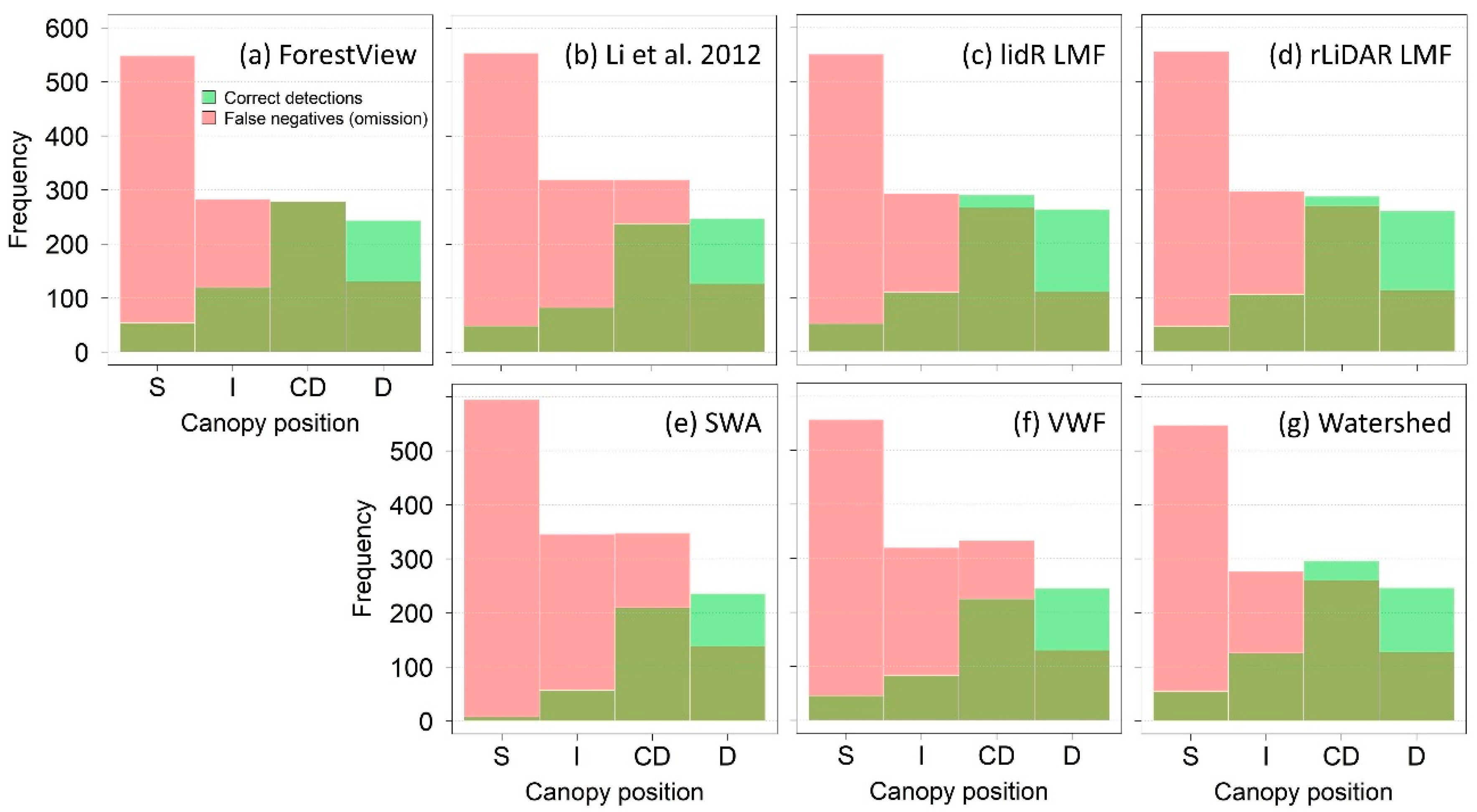
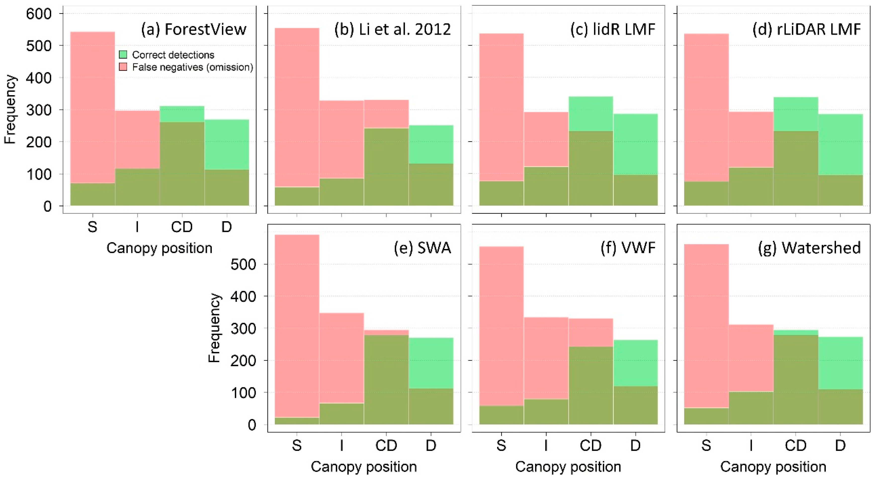
3.1. Individual Tree Detection Accuracy

The individual tree detection results are presented in

Table 4. ITD accuracy for all method approaches in terms of recall, precision, and F-score. The highest accuracy approaches for each ITD method are bolded and filled in grey. CHM = canopy height model, SW = search window.

Method and Input Parameters	8 ppm2 ALS Data			22 ppm2 ALS Data
	Recall	Precision	F-Score	Recall	Precision	F-Score
ForestView®
Default CHM and point cloud metrics	0.39	0.58	0.45	0.47	0.62	0.50
[19]
Spacing thresh: 0.75 m	0.46	0.55	0.48	0.46	0.56	0.47
Spacing thresh: 1.25 m	0.40	0.67	0.48	0.41	0.64	0.47
Spacing thresh: 1.75 m	0.35	0.73	0.46	0.37	0.67	0.45
lidR LMF
CHM: 10 cm, SW: circular 1.5 m				0.55	0.44	0.45
CHM: 10 cm, SW: circular 2.5 m				0.46	0.66	0.51
CHM: 10 cm, SW: circular 3.5 m				0.40	0.71	0.48
CHM: 10 cm, SW: square 1.5 m				0.52	0.51	0.48
CHM: 10 cm, SW: square 2.5 m				0.43	0.69	0.50
CHM: 10 cm, SW: square 3.5 m				0.37	0.72	0.46
CHM: 25 cm, SW: circular 1.5 m	0.48	0.51	0.47	0.53	0.46	0.46
CHM: 25 cm, SW: circular 2.5 m	0.41	0.71	0.51	0.45	0.66	0.51
CHM: 25 cm, SW: circular 3.5 m	0.36	0.74	0.47	0.40	0.71	0.48
CHM: 25 cm, SW: square 1.5 m	0.45	0.61	0.50	0.48	0.58	0.49
CHM: 25 cm, SW: square 2.5 m	0.38	0.73	0.49	0.42	0.70	0.49
CHM: 25 cm, SW: square 3.5 m	0.33	0.76	0.44	0.36	0.71	0.44
CHM: 50 cm, SW: circular 1.5 m	0.47	0.54	0.48	0.50	0.60	0.52
CHM: 50 cm, SW: circular 2.5 m	0.41	0.69	0.50	0.44	0.71	0.52
CHM: 50 cm, SW: circular 3.5 m	0.36	0.73	0.47	0.40	0.73	0.49
CHM: 50 cm, SW: square 1.5 m	0.47	0.54	0.48	0.50	0.60	0.52
CHM: 50 cm, SW: square 2.5 m	0.39	0.71	0.50	0.43	0.71	0.51
CHM: 50 cm, SW: square 3.5 m	0.34	0.74	0.45	0.38	0.73	0.47
rLiDAR LMF
CHM: 10 cm, SW: square 1.5 m				0.44	0.58	0.49
CHM: 10 cm, SW: square 2.5 m				0.22	0.69	0.36
CHM: 10 cm, SW: square 3.5 m				0.13	0.71	0.24
CHM: 25 cm, SW: square 1.5 m	0.41	0.63	0.49	0.44	0.63	0.50
CHM: 25 cm, SW: square 2.5 m	0.28	0.72	0.42	0.28	0.70	0.41
CHM: 25 cm, SW: square 3.5 m	0.21	0.75	0.35	0.17	0.68	0.30
CHM: 50 cm, SW: square 1.5 m	0.45	0.55	0.48	0.50	0.61	0.52
CHM: 50 cm, SW: square 2.5 m	0.35	0.71	0.47	0.38	0.72	0.49
CHM: 50 cm, SW: square 3.5 m	0.25	0.74	0.39	0.25	0.70	0.39
SWA
CHM: 10 cm				0.39	0.71	0.49
CHM: 25 cm	0.33	0.68	0.42	0.38	0.70	0.47
CHM: 50 cm	0.27	0.68	0.38	0.34	0.71	0.43
VWF
CHM: 10 cm, SW: default function				0.44	0.67	0.49
CHM: 25 cm, SW: default function	0.39	0.72	0.49	0.44	0.67	0.49
CHM: 50 cm, SW: default function	0.39	0.71	0.49	0.43	0.71	0.50
CHM: 10 cm, SW: Palouse Range function				0.33	0.71	0.42
CHM: 25 cm, SW: Palouse Range function	0.31	0.77	0.42	0.34	0.70	0.42
CHM: 50 cm, SW: Palouse Range function	0.31	0.76	0.42	0.34	0.73	0.42
Watershed
CHM: 10 cm				0.62	0.30	0.37
CHM: 25 cm	0.51	0.40	0.42	0.51	0.52	0.48
CHM: 50 cm	0.41	0.51	0.45	0.44	0.68	0.52

. Across all method approaches, recall had an average (±SD) value of 0.38 ± 0.07 using the 8 ppm² ALS data and an average of 0.41 ± 0.1 using the 22 ppm² ALS data. Precision was higher with an average value of 0.66 ± 0.1 using the 8 ppm² ALS data and an average of 0.65 ± 0.1 using the 22 ppm² ALS data.

Across all method approaches, ITD accuracy in terms of F-score increased 2.6% on average using the higher pulse density ALS data versus the lower pulse density ALS data. ForestView^®, SWA, and watershed methods benefited the most from higher pulse density ALS data, with F-scores increasing over 10% on average. Methods including [19], lidR LMF, rLiDAR LMF, and VWF benefitted the least from higher pulse density ALS data, with F-scores increasing 1.2% on average.

The highest accuracy method approaches, in terms of F-score, are highlighted in Table 4. Variation in accuracy among the top seven method approaches was low (8 ppm² ALS data F-score SD = 0.03 and 22 ppm² ALS data F-score SD = 0.02). F-score ranged from 0.42 to 0.51 for the lower pulse density ALS data and ranged from 0.47 to 0.52 for the higher pulse density data. The CHM-based fixed search window methods (lidR LMF and rLiDAR LMF) were two of the highest accuracy methods for both the low and high pulse density ALS datasets. These methods used search windows smaller than the average crown diameter for the study area (i.e., <2.5 m). The most accurate CHM-based method approaches tested using the 8 ppm² ALS data used 25 cm CHMs whereas the most accurate approaches tested using the 22 ppm² ALS data used 50 cm CHMs. The observed differences in accuracy between the different CHM resolutions were small (F-score difference of 0.01–0.02).

Omission errors, or missed trees, for all methods, regardless of ALS data, were predominately associated with intermediate and suppressed trees. The distributions of correct detections and omissions or false negatives (FN) for the seven most accurate ITD method approaches highlighted in Table 4 and derived from the 8 ppm² and 22 ppm² ALS datasets are presented in Figure 2 and Figure 3.

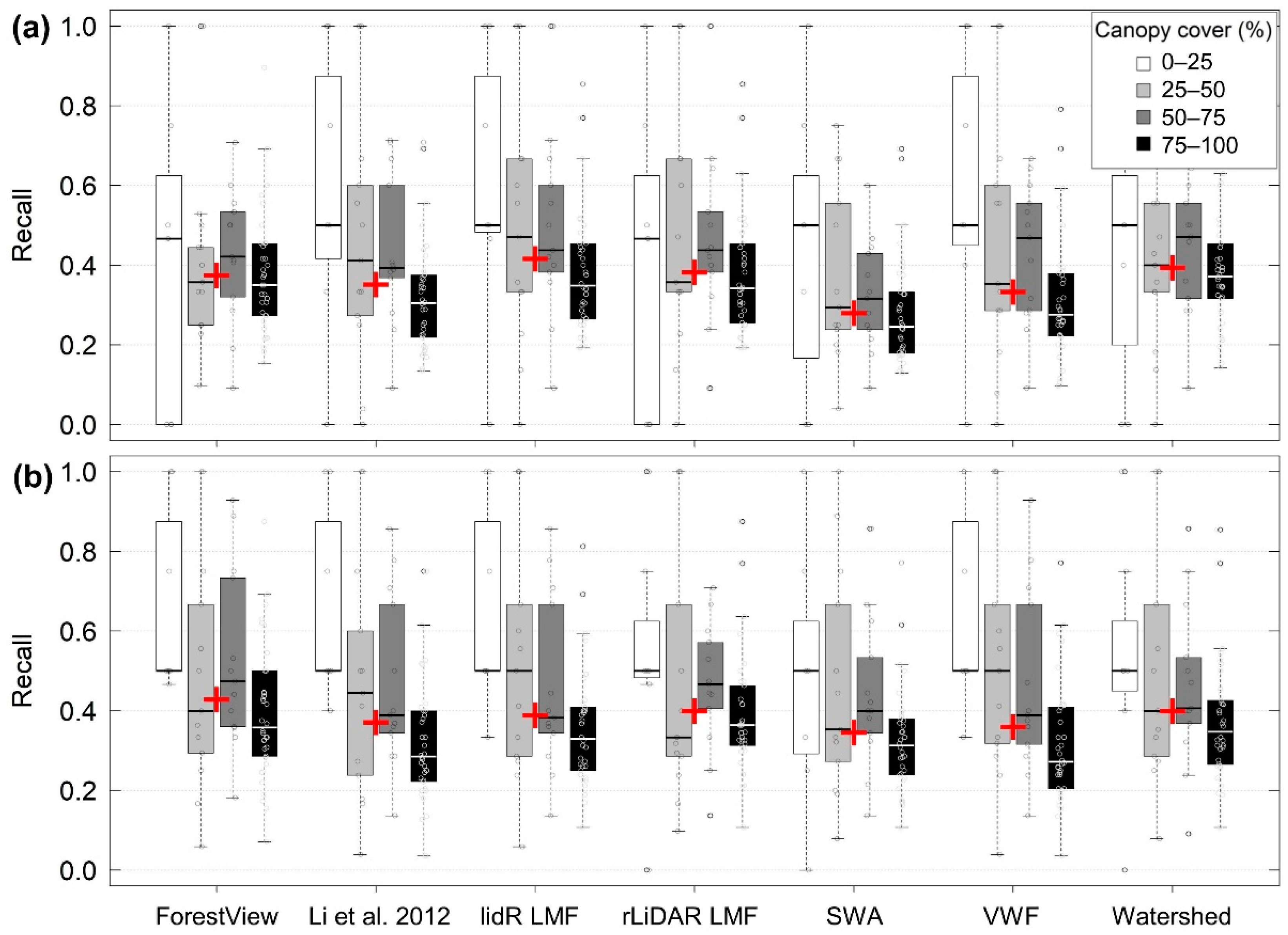
3.2. Effects of Stand Density on ITD Method Accuracy

The relationships between ITD accuracy metrics, averaged across the top seven methods for each ALS dataset, and stand density metrics are presented in

Table 5. Linear regression results between the top ITD method accuracies, averaged to the plot scale, and stand density metrics.

Accuracy Metric	Canopy Cover			Trees per Hectare			Basal Area per Hectare			Stand Density Index
	r2	Slope	p	r2	Slope	p	r2	Slope	p	r2	Slope	p
8 ppm2 ALS dataset
Recall	0.05	−0.15	0.07	0.19	−0.0002	<0.01	0.16	−0.003	<0.01	0.20	−0.0002	<0.01
Precision	0.01	0.06	0.43	0.07	0.0001	<0.05	0.01	−0.0002	0.82	0.01	−0.0001	0.87
F−score	0.08	−0.16	<0.05	0.14	−0.0001	<0.01	0.19	−0.003	<0.01	0.21	−0.0001	<0.01
RMSEhgt	0.01	−0.05	0.66	0.03	−0.0001	0.17	0.02	−0.001	0.28	0.02	−0.0001	0.22
Biashgt	0.02	0.33	0.22	0.01	0.0001	0.49	0.20	0.01	<0.01	0.16	0.0005	<0.01
22 ppm2 ALS dataset
Recall	0.16	−0.29	<0.01	0.27	−0.0002	<0.01	0.38	−0.006	<0.01	0.40	−0.0003	<0.01
Precision	0.01	−0.002	0.98	0.02	−0.0001	0.19	0.02	−0.001	0.17	0.01	−0.0005	0.36
F−score	0.08	−0.21	<0.05	0.13	−0.0001	<0.01	0.30	−0.004	<0.01	0.30	−0.0002	<0.01
RMSEhgt	0.07	0.26	<0.05	0.03	0.0001	0.16	0.23	0.005	<0.01	0.20	0.0002	<0.01
Biashgt	0.07	0.42	<0.05	0.03	0.0002	0.13	0.20	0.009	<0.01	0.17	0.0004	<0.01

. Recall for all ITD methods decreased with increasing stand density, implying higher omission errors in denser stands. Average recall for the top seven methods had negative relationships with all stand density metrics (Table 5). Recall for the top seven method approaches stratified by canopy cover is presented in Figure 4. Precision was poorly related (r² < 0.07) with all of the stand density metrics (Table 5).

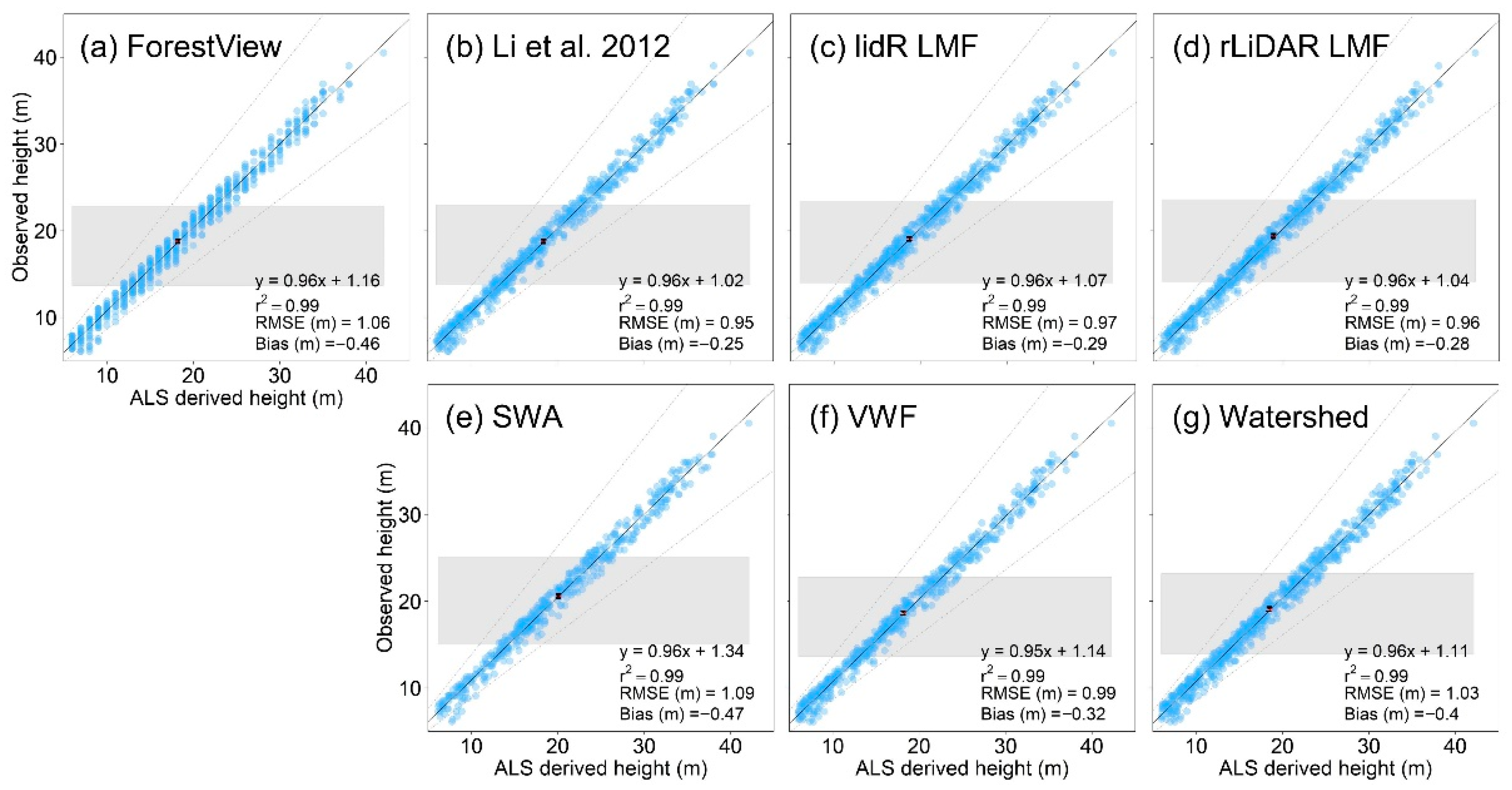
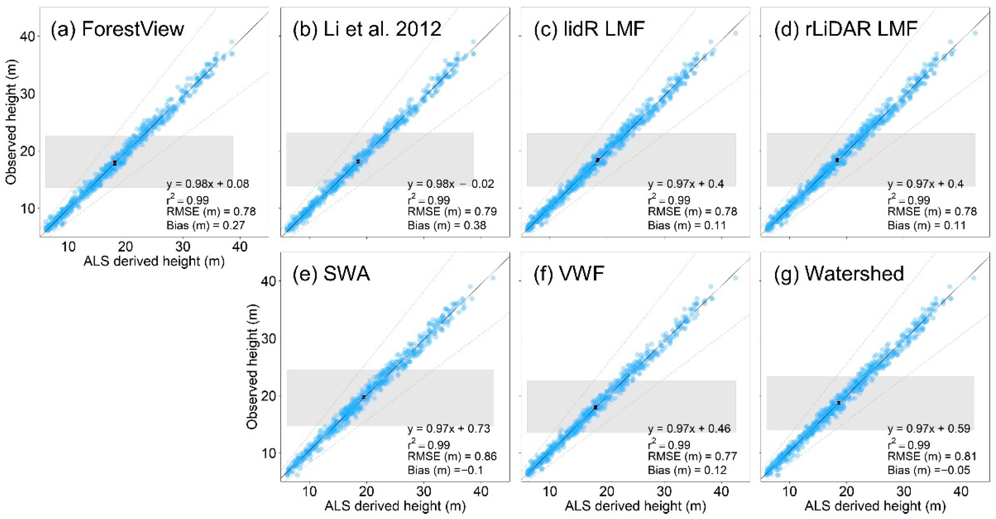
3.3. ITD Method Height Measurement Accuracy

The average height measurement RMSE for the top ITD method approaches derived from the 8 ppm² ALS dataset was 1.01 ± 0.05 m and average bias was −0.35 ± 0.09 m. Height bias was positively correlated with both basal area per hectare (r² = 0.20, p < 0.01) and stand density index (r² = 0.16, p < 0.01) (Table 5). The average height measurement RMSE for the top method approaches derived from the 22 ppm² ALS dataset was 0.80 ± 0.03 m with an average bias of 0.12 ±0.17 m. Height RMSE was positively related to basal area per hectare (r² = 0.23, p < 0.01) and stand density index (r² = 0.20, p < 0.01) (Table 5). Likewise, height bias had positive relationships with both basal area per hectare (r² = 0.20, p < 0.01) and stand density index (r² = 0.17, p< 0.01).

Figure 5 and Figure 6 present results from the regression-based equivalence tests. For all paired datasets (top ITD methods using 8 ppm² ALS data vs. reference and top methods using ALS 22 ppm² data vs. reference), the 95% confidence interval for the intercept (vertical grey bar) was within the ±25% region of equivalence (grey polygon), indicating that the null hypothesis of dissimilarity can be rejected (i.e., paired datasets are equivalent). Likewise, for all paired datasets, the 95% confidence interval for the slope (vertical black bar) was within the ±25% region of equivalence (grey dashed lines), indicating slopes were significantly similar to 1.

4. Discussion

This study sought to cross-compare seven different ITD approaches with reference to a common validation dataset and as we expand on below, ITD accuracy metrics that account for both omission and commission errors (e.g., F-score) did not vary considerably by method. Notably, despite the diversity of the applied methods and parameters, the results were broadly similar with comparable accuracies obtained. While F-score was similar across the methods, detection rates, or the proportion of reference trees that were detected, did vary by canopy position across methods. All methods had similar detection rates of dominant trees but ForestView^®, lidR LMF, rLiDAR LMF, and watershed methods had greater detection rates for codominant and subdominant trees (intermediate and suppressed). For applications where dominant trees are the focus, it could be argued that the selection of a specific ITD method is somewhat arbitrary and may rely more on user preference. This is important, as it means that more research can focus on exploring the applications regardless of the specific selected approach and cross-comparisons of application studies that use different ITD methods may be more readily achievable than previously considered. Such applications can include, but are not limited to: quantifying wildlife habitats [58,59,60]; assessing crown fire risk [61,62]; reducing uncertainties associated with estimating carbon stocks due to forest crown consumption through exploring the relative number of tree crowns that form standing dead biomass (snags) versus the formation of fallen large woody debris following fires [63,64,65]; developing new allometric relations using structural datasets and reducing uncertainties in the stand to landscape scale assessments in carbon monitoring, forest growth, and yield [10,66,67]; assessing structural metrics of fire severity [68,69,70,71]; assessing metrics of ecosystem vulnerability [72]; and mapping urban forests [73].

Overall, F-score accuracies varied little between the different methods, ranging from 0.42 to 0.51 for the 8 ppm² ALS data and 0.47 to 0.52 for the 22 ppm² ALS data with regard to the top seven best performing methods. This similarity is likely influenced by the consistent ‘top-down’ approach of the methods, where dominant overstory trees are identified but many subdominant trees are occluded by overstory canopies. ITD accuracy increased with increasing pulse density across all methods, regardless of method type (point-cloud-based, raster-based, hybrid). This is in contrast with several prior studies where increasing pulse density increased ITD accuracy for mainly point-cloud-based methods and not raster-based methods [18] and those that did not observe a significant effect of increasing pulse density on ITD accuracy [16]. While ITD accuracy increased with increasing pulse density, results show that some methods (ForestView^®, SWA, watershed) benefited more than other methods ([19], lidR LMF, rLiDAR LMF, VWF).

In part due to the top-down design of the assessed methods, most undetected trees (omission errors) were in intermediate and suppressed canopy positions (Figure 2 and Figure 3). All seven top ITD methods detected most dominant trees (66% on average for 8 ppm² ALS dataset and 71% on average for the 22 ppm² ALS dataset). Only ForestView^®, lidR LMF, rLiDAR LMF, and watershed detected a majority of codominant trees using both ALS datasets. Other benchmarking studies using similar ITD methods observed higher detection for dominant (85%) and codominant trees (70%) [18], although stand density was lower (median: 353 trees hectare⁻¹) than the stands assessed in this study (median: 509 trees hectare⁻¹). Additionally, the stand composition, crown shape variation, and structural heterogeneity in the study area were likely greater than many prior benchmark studies given the higher number of species and diverse management history. Across all methods and for both ALS datasets, detection of intermediate trees was less than 31% and detection of suppressed trees was less than 13%. This is the direct result of trees in subdominant canopy positions being occluded by the dominant forest canopy [32,33]. Detection of dominant and codominant trees using the 22 ppm² ALS dataset was 4% higher on average, compared to methods using the 8 ppm² data. Higher detection rates using ALS datasets with higher pulse densities have been observed in other North American and European forests (e.g., [18,74]), but in some cases higher pulse density has not improved ITD [16]. CHM-based top ITD methods that used a fixed search window size (lidR LMF and rLiDAR LMF) achieved the highest detection across all canopy classes using the 22 ppm² ALS dataset and performed well using the 8 ppm² ALS dataset. Other ITD method comparisons have also found that simple local maximum-finding can be one of the most accurate and easy-to-implement methods [16,17]. However, these simple raster-based methods may not perform as well as point-cloud-based methods for subcanopy tree detection [18,74].

There was large intra-method accuracy variability depending on the input datasets and parameters. ITD methods that used spacing thresholds (i.e., [19]) or LMF search window sizes (i.e., lidR LMF, rLiDAR LMF) smaller than the average crown diameter tended to have higher commission error, while those with larger thresholds/windows tended to have higher omission error. Generally, ITD methods that used spacing thresholds or LMF search window sizes that were equal to or less than the average crown diameter for study area trees (2.5 m) were the most accurate. While most raster-based ITD methods applied to the 8 ppm² ALS data produced improved results with a 25 cm CHM over a 50 cm CHM, the difference was minimal (average F-score difference < 1%). Likewise, most CHM-based ITD methods using the 22 ppm² ALS data produced more accurate results when applied to a 50 cm CHM than to a 25 cm CHM, but the difference was small (average F-score difference < 4%). These particular accuracy results may be owing to differences in the pulse density created by the differing scanning patterns of the two ALS datasets. The 2018 dataset was acquired in a sawtooth, or ‘zig-zag’, pattern and likely has higher pulse density at the edges of flight paths where scans overlap and lower pulse density in between flight paths. The 2021 dataset was acquired in an equidistant pulse-spread, or ‘matrix’, scan that produces more consistent pulse densities across the flight path. We did not apply any point cloud thinning methods to homogenize the pulse density across either of the point clouds, but clearly this is an issue that should be explored in future work as pulse density can have significant effects on individual tree detection accuracy [18,34].

Like other ITD method comparison studies (e.g., [4,31]), stand density was a larger driver of method accuracy than the individual methods themselves. Typically, as stand density increases, space in between tree crowns decreases and more overlapping tree crowns are present, complicating identification of individual trees. Additionally, as the dominant forest canopy increases in density, more subdominant smaller trees are likely to become occluded, except where gaps within the canopy occur [32,33]. This suggests that non-raster-based ITD methods that operate directly on the ALS point cloud may be better suited for denser forest conditions [18,75].

All of the ITD methods produced height measurements for the detected trees that had low RMSE (<1.1 m) and bias (<0.5 m). Height bias was larger for methods using the 8 ppm² ALS dataset (mean bias: −0.35 m) than for the 22 ppm² dataset (mean bias: 0.12 m). The larger bias observed for the 8 ppm² ALS dataset is likely due in part to tree growth between the dates of ALS acquisition (2018) and reference-tree field data collection (2020). Generally, the mean height growth of mature mixed conifer species present within this study area is 0.4 m per year [39]. Regardless, all methods using either of the ALS datasets produced tree heights that were statistically similar to the reference tree heights.

This study primarily focused on assessing methods that use a ‘top-down’ approach to identify individual trees. The findings of this research outline the need for future benchmarking to include methods that utilize a ‘bottom-up’ approach (e.g., layer stacking methods in [20]) and methods that create separate CHMs for dominant and subdominant trees (e.g., [25]). However, it should be noted that detection rates of intermediate and suppressed trees (35% and 21%, respectively) reported in Duncanson et al. [25] are not substantially higher than those obtained by the ‘top-down’ methods in this study (31% of intermediate trees and 13% of suppressed trees).

5. Conclusions

This study assessed the individual tree detection and height measurement accuracy of different tree detection approaches via comparison with a benchmark dataset with diverse structure and composition. Generally, stand density and canopy cover were larger drivers of ITD accuracy than ITD method choice. However, results show that detection of trees in certain canopy positions can vary by method. All methods detected most trees with dominant canopy positions but ForestView^®, lidR LMF, rLiDAR LMF, and watershed methods had the highest detection proportion of codominant and subdominant trees and CHM-based local-maximum filter methods had the lowest omission errors across all tree canopy positions. This study additionally supports the value of ALS data with pulse densities > 8 ppm² for ITD, given higher pulse density data increased average F-scores by 10% for ForestView^®, SWA, and watershed methods and 1.2% for [19], lidR LMF, rLiDAR LMF, and the VWF methods. The results emphasize the importance of input parameter selection when applying ITD methods, as intra-method ITD accuracy variability was large depending on data and parameter selection. For CHM-based methods, ITD accuracy was generally highest using finer resolution CHMs (~25 cm) when lower pulse density ALS data (8 ppm²) were available, which contrasted with CHM-based ITD results when higher pulse density ALS data were available (22 ppm² and a 50 cm resolution CHM). Likewise, CHM-based methods that utilized fixed size search windows achieved the highest accuracy with sizes equal to or less than the average tree crown diameter. All methods were comparable in terms of height measurements for the detected trees, but errors increased with increasing stand density. The results presented here should help end-users with the choice and application of these and similar ITD methods on available ALS datasets. Future benchmarking studies for ITD methods should consider more diverse methods (e.g., bottom-up approaches) that detect more subdominant trees and explore the influence of ALS scanning patterns (e.g., oscillating mirror vs. rotating polygonal mirror) on ITD accuracy.

References

1. Luoma, V.; Saarinen, N.; Wulder, M.A.; White, J.C.; Vastaranta, M.; Holopainen, M.; Hyyppä, J. Assessing precision in conventional field measurements of individual tree attributes. Forests 2017, 8, 38. [Google Scholar] [CrossRef] [Green Version]
2. Durrieu, S.; Vega, C.; Bouvier, M.; Gosselin, F.; Renaud, J.P.; Saint-Andre, L. Optical remote sensing of tree and stand heights. In Land Resources Monitoring, Modeling, and Mapping with Remote Sensing; CRC Press: Boca Raton, FL, USA, 2015; pp. 449–485. [Google Scholar] [CrossRef]
3. Persson, A.; Holmgren, J.; Söderman, U. Detecting and Measuring Individual Trees Using an Airborne Laser Scanner. Photogram. Eng. Remote Sens. 2002, 68, 925–932. [Google Scholar]
4. Falkowski, M.J.; Smith, A.M.S.; Gessler, P.E.; Hudak, A.T.; Vierling, L.A.; Evans, J.S. The influence of conifer forest canopy cover on the accuracy of two individual tree measurement algorithms using lidar data. Can. J. Remote Sens. 2008, 34, S338–S350. [Google Scholar] [CrossRef]
5. Dalla Corte, A.P.; Souza, D.V.; Rex, F.E.; Sanquetta, C.R.; Mohan, M.; Silva, C.A.; Zambrano, A.M.A.; Prata, G.; de Almeida, D.R.A.; Trautenmüller, J.W.; et al. Forest inventory with high-density UAV-Lidar: Machine learning approaches for predicting individual tree attributes. Comput. Electron. Agric. 2020, 179, 105815. [Google Scholar] [CrossRef]
6. Tatum, J.; Wallin, D. Using Discrete-Point LiDAR to Classify Tree Species in the Riparian Pacific Northwest, USA. Remote Sens. 2021, 13, 2647. [Google Scholar] [CrossRef]
7. Borgogno Mondino, E.; Fissore, V.; Falkowski, M.J.; Palik, B. How far can we trust forestry estimates from low-density LiDAR acquisitions? The Cutfoot Sioux experimental forest (MN, USA) case study. Int. J. Remote Sens. 2020, 41, 4551–4569. [Google Scholar] [CrossRef]
8. Corrao, M.V.; Sparks, A.M.; Smith, A.M.S. A Conventional Cruise and Felled-Tree Validation of Individual Tree Diameter, Height and Volume Derived from Airborne Laser Scanning Data of a Loblolly Pine (P. taeda) Stand in Eastern Texas. Remote Sens. 2022, 14, 2567. [Google Scholar] [CrossRef]
9. Sparks, A.M.; Smith, A.M.S. Accuracy of a LiDAR-Based Individual Tree Detection and Attribute Measurement Algorithm Developed to Inform Forest Products Supply Chain and Resource Management. Forests 2022, 13, 3. [Google Scholar] [CrossRef]
10. Tinkham, W.T.; Smith, A.M.S.; Affleck, D.L.; Saralecos, J.D.; Falkowski, M.J.; Hoffman, C.M.; Hudak, A.T.; Wulder, M.A. Development of height-volume relationships in second growth Abies grandis for use with aerial LiDAR. Can. J. Remote Sens. 2016, 42, 400–410. [Google Scholar] [CrossRef]
11. Jeronimo, S.M.A.; Kane, V.R.; Churchill, D.J.; McGaughey, R.J.; Franklin, J.F. Applying LiDAR individual tree detection to management of structurally diverse forest landscapes. J. For. 2018, 116, 336–346. [Google Scholar] [CrossRef] [Green Version]
12. Tinkham, W.T.; Mahoney, P.R.; Smith, A.M.S.; Falkowski, M.J.; Woodall, C.; Donke, G.; Hudak, A.T. Applications of the United States Forest Service Forest Inventory and Analysis dataset: A review and future directions. Can. J. For. Res. 2018, 48, 1251–1268. [Google Scholar] [CrossRef]
13. Duncanson, L.; Dubayah, R. Monitoring individual tree-based change with airborne lidar. Ecol. Evol. 2018, 8, 5079–5089. [Google Scholar] [CrossRef] [PubMed]
14. Keefe, R.F.; Zimbelman, E.G.; Picchi, G. Use of Individual Tree and Product Level Data to Improve Operational Forestry. Curr. For. Rep. 2022, 8, 148–165. [Google Scholar] [CrossRef]
15. Larsen, M.; Eriksson, M.; Descombes, X.; Perrin, G.; Brandtberg, T.; Gougeon, F.A. Comparison of six individual tree crown detection algorithms evaluated under varying forest conditions. Int. J. Remote Sens. 2011, 32, 5827–5852. [Google Scholar] [CrossRef]
16. Kaartinen, H.; Hyyppä, J.; Yu, X.; Vastaranta, M.; Hyyppä, H.; Kukko, A.; Holopainen, M.; Heipke, C.; Hirschmugl, M.; Morsdorf, F.; et al. An international comparison of individual tree detection and extraction using airborne laser scanning. Remote Sens. 2012, 4, 950–974. [Google Scholar] [CrossRef] [Green Version]
17. Eysn, L.; Hollaus, M.; Lindberg, E.; Berger, F.; Monnet, J.M.; Dalponte, M.; Kobal, M.; Pellegrini, M.; Lingua, E.; Mongus, D.; et al. A benchmark of lidar-based single tree detection methods using heterogeneous forest data from the alpine space. Forests 2015, 6, 1721–1747. [Google Scholar] [CrossRef] [Green Version]
18. Wang, Y.; Hyyppä, J.; Liang, X.; Kaartinen, H.; Yu, X.; Lindberg, E.; Holmgren, J.; Qin, Y.; Mallet, C.; Ferraz, A.; et al. International benchmarking of the individual tree detection methods for modeling 3-D canopy structure for silviculture and forest ecology using airborne laser scanning. IEEE Trans. Geosci. Remote Sens. 2016, 54, 5011–5027. [Google Scholar] [CrossRef] [Green Version]
19. Li, W.; Guo, Q.; Jakubowski, M.K.; Kelly, M. A new method for segmenting individual trees from the lidar point cloud. Photogram. Eng. Remote Sens. 2012, 10, 75–84. [Google Scholar] [CrossRef] [Green Version]
20. Ayrey, E.; Fraver, S.; Kershaw, J.A., Jr.; Kenefic, L.S.; Hayes, D.; Weiskittel, A.R.; Roth, B.E. Layer stacking: A novel algorithm for individual forest tree segmentation from LiDAR point clouds. Can. J. Remote Sens. 2017, 43, 16–27. [Google Scholar] [CrossRef]
21. Hyyppä, J.; Schardt, M.; Haggrén, H.; Koch, B.; Lohr, U.; Scherrer, H.U.; Paananen, R.; Luukkonen, H.; Ziegler, M.; Hyyppä, H.; et al. HIGH-SCAN: The first European-wide attempt to derive single-tree information from laserscanner data. Photogramm. J. Finl. 2001, 17, 58–68. [Google Scholar]
22. Popescu, S.C.; Wynne, R.H. Seeing the trees in the forest. Photogram. Eng. Remote Sens. 2004, 16, 589–604. [Google Scholar] [CrossRef] [Green Version]
23. Falkowski, M.J.; Smith, A.M.S.; Hudak, A.T.; Gessler, P.E.; Vierling, L.A.; Crookston, N.L. Automated estimation of individual conifer tree height and crown diameter via two-dimensional spatial wavelet analysis of lidar data. Can. J. Remote Sens. 2006, 32, 153–161. [Google Scholar] [CrossRef] [Green Version]
24. Silva, C.A.; Hudak, A.T.; Vierling, L.A.; Loudermilk, E.L.; O’Brien, J.J.; Hiers, J.K.; Jack, S.B.; Gonzalez-Benecke, C.; Lee, H.; Falkowski, M.J.; et al. Imputation of individual longleaf pine (Pinus palustris Mill.) tree attributes from field and LiDAR data. Can. J. Remote Sens. 2016, 42, 554–573. [Google Scholar] [CrossRef]
25. Duncanson, L.I.; Cook, B.D.; Hurtt, G.C.; Dubayah, R.O. An efficient, multi-layered crown delineation algorithm for mapping individual tree structure across multiple ecosystems. Remote Sens. Environ. 2014, 154, 378–386. [Google Scholar] [CrossRef]
26. Zhen, Z.; Quackenbush, L.J.; Zhang, L. Trends in automatic individual tree crown detection and delineation—Evolution of LiDAR data. Remote Sens. 2016, 8, 333. [Google Scholar] [CrossRef] [Green Version]
27. Lindberg, E.; Holmgren, J. Individual Tree Crown Methods for 3D Data from Remote Sensing. Curr. For. Rep. 2017, 3, 19–31. [Google Scholar] [CrossRef] [Green Version]
28. Mohan, M.; Silva, C.A.; Klauberg, C.; Jat, P.; Catts, G.; Cardil, A.; Hudak, A.T.; Dia, M. Individual tree detection from unmanned aerial vehicle (UAV) derived canopy height model in an open canopy mixed conifer forest. Forests 2017, 8, 340. [Google Scholar] [CrossRef] [Green Version]
29. Leite, R.V.; Amaral, C.H.D.; Pires, R.D.P.; Silva, C.A.; Soares, C.P.B.; Macedo, R.P.; Silva, A.A.L.D.; Broadbent, E.N.; Mohan, M.; Leite, H.G. Estimating stem volume in eucalyptus plantations using airborne LiDAR: A comparison of area-and individual tree-based approaches. Remote Sens. 2020, 12, 1513. [Google Scholar] [CrossRef]
30. Kolendo, Ł.; Kozniewski, M.; Ksepko, M.; Chmur, S.; Neroj, B. Parameterization of the Individual Tree Detection Method Using Large Dataset from Ground Sample Plots and Airborne Laser Scanning for Stands Inventory in Coniferous Forest. Remote Sens. 2021, 13, 2753. [Google Scholar] [CrossRef]
31. Vauhkonen, J.; Ene, L.; Gupta, S.; Heinzel, J.; Holmgren, J.; Pitkänen, J.; Solberg, S.; Wang, Y.; Weinacker, H.; Hauglin, K.M.; et al. Comparative testing of single-tree detection algorithms under different types of forest. Forestry 2012, 85, 27–40. [Google Scholar] [CrossRef] [Green Version]
32. Hyyppa, J.; Kelle, O.; Lehikoinen, M.; Inkinen, M. A segmentation-based method to retrieve stem volume estimates from 3-D tree height models produced by laser scanners. IEEE Trans. Geosci. Remote Sens. 2001, 39, 969–975. [Google Scholar] [CrossRef]
33. White, J.C.; Coops, N.C.; Wulder, M.A.; Vastaranta, M.; Hilker, T.; Tompalski, P. Remote sensing technologies for enhancing forest inventories: A review. Can. J. Remote Sens. 2016, 42, 619–641. [Google Scholar] [CrossRef] [Green Version]
34. Pearse, G.D.; Watt, M.S.; Dash, J.P.; Stone, C.; Caccamo, G. Comparison of models describing forest inventory attributes using standard and voxel-based lidar predictors across a range of pulse densities. Int. J. Appl. Earth Obs. Geoinf. 2019, 78, 341–351. [Google Scholar] [CrossRef]
35. Eitel, J.U.; Höfle, B.; Vierling, L.A.; Abellán, A.; Asner, G.P.; Deems, J.S.; Glennie, C.L.; Joerg, P.C.; LeWinter, A.L.; Magney, T.S.; et al. Beyond 3-D: The new spectrum of lidar applications for earth and ecological sciences. Remote Sens. Environ. 2016, 186, 372–392. [Google Scholar] [CrossRef] [Green Version]
36. Roussel, J.R.; Auty, D.; Coops, N.C.; Tompalski, P.; Goodbody, T.R.; Meador, A.S.; Bourdon, J.F.; de Boissieu, F.; Achim, A. lidR: An R package for analysis of Airborne Laser Scanning (ALS) data. Remote Sens. Environ. 2020, 251, 112061. [Google Scholar] [CrossRef]
37. McGaughey, R.J. FUSION/LDV: Software for LIDAR Data Analysis and Visualization. USDA Forest Service, Pacific Northwest Research Station. 2022. Available online: http://forsys.cfr.washington.edu/fusion/fusion_overview.html (accessed on 11 April 2022).
38. Smith, A.M.S.; Falkowski, M.J.; Hudak, A.T.; Evans, J.S.; Robinson, A.P.; Steele, C.M. A cross-comparison of field, spectral, and lidar estimates of forest canopy cover. Can. J. Remote Sens. 2009, 35, 447–459. [Google Scholar] [CrossRef]
39. Hudak, A.T.; Strand, E.K.; Vierling, L.A.; Byrne, J.C.; Eitel, J.U.H.; Martinuzzi, S.; Falkiwski, M.J. Quantifying aboveground forest carbon pools and fluxes from repeat LiDAR surveys. Remote Sens. Environ. 2012, 123, 25–40. [Google Scholar] [CrossRef] [Green Version]
40. United States Geological Survey. Lidar Base Specification Version 2.1. 2019. Available online: https://www.usgs.gov/3DEP/lidarspec (accessed on 6 June 2022).
41. Kraft, G. Beiträge zur Lehre von den Durchforstungen, Schlagstellungen und Lichtungshieben; Klindsworth’s Verlag: Hannover, Germany, 1884. [Google Scholar]
42. Silva, C.A.; Crookston, N.L.; Hudak, A.T.; Vierling, L.A. rLiDAR: An R Package for Reading, Processing and Visualizing LiDAR (Light Detection and Ranging) Data, Version 0.1.5. 2021. Available online: https://cran.r-project.org/web/packages/rLiDAR/index.html (accessed on 11 April 2022).
43. Plowright, A.; Roussel, J. Forest Tools. R Package Version 0.2.5. 2019. Available online: https://github.com/andrew-plowright/ForestTools (accessed on 20 January 2022).
44. Garrity, S.R.; Vierling, L.A.; Smith, A.M.S.; Hann, D.B.; Falkowski, M.J. Automatic detection of shrub location, crown area, and cover using spatial wavelet analysis and aerial photography. Can. J. Remote Sens. 2008, 34, S376–S384. [Google Scholar] [CrossRef]
45. Poznanovic, A.J.; Falkowski, M.J.; MacLean, A.L.; Evans, J.S.; Smith, A.M.S. An accuracy assessment of tree detection algorithms in juniper woodlands. Photogram. Eng. Remote Sens. 2014, 80, 45–55. [Google Scholar] [CrossRef]
46. Smith, A.M.S.; Strand, E.K.; Steele, C.M.; Hann, D.B.; Garrity, S.R.; Falkowski, M.J.; Evans, J.S. Production of vegetation spatial-structure maps by per-object analysis of juniper encroachment in multi-temporal aerial photographs. Can. J. Remote Sens. 2008, 34, S268–S285. [Google Scholar] [CrossRef] [Green Version]
47. Strand, E.K.; Smith, A.M.S.; Bunting, S.C.; Vierling, L.A.; Hann, D.B.; Gessler, P.E. Wavelet estimation of plant spatial patterns in multi-temporal aerial photography. Int. J. Remote Sens. 2006, 27, 2049–2054. [Google Scholar] [CrossRef]
48. Strand, E.K.; Vierling, L.A.; Smith, A.M.S.; Bunting, S.C. Net Changes in Above Ground Woody Carbon Stock in Western Juniper Woodlands, 1946–1998. J. Geophys. Res. 2008, 113, G01013. [Google Scholar] [CrossRef] [Green Version]
49. Vincent, L.; Soille, P. Watersheds in digital spaces: An efficient algorithm based on immersion simulations. IEEE Trans. Patt. Analys. Mach. Intel. 1991, 13, 583–598. [Google Scholar] [CrossRef] [Green Version]
50. Khosravipour, A.; Skidmore, A.K.; Isenburg, M.; Wang, T.; Hussin, Y.A. Generating pit-free canopy height models from airborne lidar. Photogram. Eng. Remote Sens. 2014, 80, 863–872. [Google Scholar] [CrossRef]
51. Yang, Q.; Su, Y.; Jin, S.; Kelly, M.; Hu, T.; Ma, Q.; Li, Y.; Song, S.; Zhang, J.; Xu, G.; et al. The influence of vegetation characteristics on individual tree segmentation methods with airborne LiDAR data. Remote Sens. 2019, 11, 2880. [Google Scholar] [CrossRef] [Green Version]
52. Vastaranta, M.; Saarinen, N.; Kankare, V.; Holopainen, M.; Kaartinen, H.; Hyyppä, J.; Hyyppä, H. Multisource single-tree inventory in the prediction of tree quality variables and logging recoveries. Remote Sens. 2014, 6, 3475–3491. [Google Scholar] [CrossRef] [Green Version]
53. Pentz, M.; Shott, M. Handling Experimental Data; Open University Press: Maidenhead, UK, 1988; ISBN 12-978-0335158973. [Google Scholar]
54. Burkhart, H.E.; Tomé, M. Modeling Forest Trees and Stands; Springer Science & Business Media: New York, NY, USA, 2012. [Google Scholar]
55. Robinson, A.P.; Duursma, R.A.; Marshall, J.D. A regression-based equivalence test for model validation: Shifting the burden of proof. Tree Phys. 2005, 25, 903–913. [Google Scholar] [CrossRef]
56. R Core Team. R: A Language and Environment for Statistical Computing; R Foundation for Statistical Computing: Vienna, Austria, 2022; Available online: https://www.R-project.org (accessed on 6 June 2022).
57. Robinson, A. Equivalence: Provides Tests and Graphics for Assessing Tests of Equivalence, Version 0.7.2. 2016. Available online: https://cran.r-project.org/web/packages/equivalence (accessed on 24 January 2022).
58. Hudak, A.T.; Evans, J.S.; Smith, A.M.S. Review: LiDAR Utility for Natural Resource Managers. Remote Sens. 2009, 1, 934–951. [Google Scholar] [CrossRef] [Green Version]
59. Martinuzzi, S.; Vierling, L.A.; Gould, W.A.; Falkowski, M.J.; Evans, J.S.; Hudak, A.T.; Vierling, K.T. Mapping snags and understory shrubs for a LiDAR-based assessment of wildlife habitat suitability. Remote Sens. Environ. 2009, 113, 2533–2546. [Google Scholar] [CrossRef] [Green Version]
60. Casas, A.; Garcia, M.; Siegel, R.B.; Koltunov, A.; Ramirez, C.; Ustin, S. Burned forest characterization at single-tree level with airborne laser scanning for assessing wildlife habitat. Remote Sens. Environ. 2016, 175, 231–241. [Google Scholar] [CrossRef] [Green Version]
61. Kramer, H.A.; Collins, B.M.; Kelly, M.; Stephens, S.L. Quantifying Ladder Fuels: A New Approach Using LiDAR. Forests 2014, 5, 1432–1453. [Google Scholar] [CrossRef]
62. Olszewski, J.H.; Bailey, J.D. LiDAR as a Tool for Assessing Change in Vertical Fuel Continuity Following Restoration. Forests 2022, 13, 503. [Google Scholar] [CrossRef]
63. Stenzel, J.E.; Bartowitz, K.J.; Hartman, M.D.; Lutz, J.A.; Smith, A.M.S.; Kolden, C.A.; Law, B.E.; Swanson, M.E.; Larson, A.J.; Parton, W.J.; et al. Fixing a snag in estimating carbon emissions from wildfires. Glob. Change Biol. 2019, 25, 3985–3994. [Google Scholar] [CrossRef] [PubMed]
64. Jarron, L.R.; Coops, N.C.; MacKenzie, W.H.; Dykstra, P. Detection and Quantification of Coarse Woody Debris in Natural Forest Stands Using Airborne LiDAR. For. Sci. 2021, 67, 550–563. [Google Scholar] [CrossRef]
65. Hanan, E.J.; Kennedy, M.C.; Ren, J.; Johnson, M.C.; Smith, A.M.S. Missing climate feedbacks in fire models: Limitations and uncertainties in fuel loadings and the role of decomposition in fine fuel succession. J. Adv. Model. Earth Sys. 2022, 14, e2021MS002818. [Google Scholar] [CrossRef]
66. Falkowski, M.J.; Hudak, A.T.; Crookston, N.; Gessler, P.E.; Ubeler, E.H.; Smith, A.M.S. Landscape-scale parameterization of a tree-level forest growth model: A k-NN imputation approach incorporating LiDAR data. Can. J. For. Res. 2010, 40, 184–199. [Google Scholar] [CrossRef]
67. Hudak, A.T.; Fekety, P.A.; Kane, V.R.; Kennedy, R.E.; Filippelli, S.K.; Falkowski, M.J.; Tinkham, W.T.; Smith, A.M.S.; Crookston, N.L.; Domke, G.M.; et al. A carbon monitoring system for mapping regional, annual aboveground biomass across the northwestern USA. Environ. Res. Lett. 2020, 15, 095003. [Google Scholar] [CrossRef]
68. McCarley, T.R.; Kolden, C.A.; Vaillant, N.M.; Hudak, A.T.; Smith, A.M.S.; Wing, B.M.; Kellogg, B.S.; Kreitler, J. Multi-temporal LiDAR and Landsat quantification of fire-induced changes to forest structure. Remote Sens. Environ. 2017, 191, 419–432. [Google Scholar] [CrossRef] [Green Version]
69. McCarley, T.R.; Kolden, C.A.; Vaillant, N.M.; Hudak, A.T.; Smith, A.M.S.; Kreitler, J. Landscape-scale quantification of fire-induced change in canopy cover following mountain pine beetle outbreak and timber harvest. For. Ecol. Manag. 2017, 391, 164–175. [Google Scholar] [CrossRef] [Green Version]
70. Hu, T.; Ma, Q.; Su, Y.; Battles, J.J.; Collins, B.M.; Stephens, S.L.; Kelly, M.; Gui, Q. A simple and integrated approach for fire severity assessment using bi-temporal airborne LiDAR data. Int. J. Appl. Earth Obs. Geoinf. 2019, 78, 25–38. [Google Scholar] [CrossRef]
71. Hillman, S.; Hally, B.; Wallace, L.; Turner, D.; Lucieer, A.; Reinke, K.; Jones, S. High-Resolution Estimates of Fire Severity—An Evaluation of UAS Image and LiDAR Mapping Approaches on a Sedgeland Forest Boundary in Tasmania, Australia. Fire 2021, 4, 14. [Google Scholar] [CrossRef]
72. Smith, A.M.S.; Kolden, C.A.; Tinkham, W.T.; Talhelm, A.F.; Marshall, J.D.; Hudak, A.T.; Boschetti, L.; Falkowski, M.J.; Greenberg, J.A.; Anderson, J.W.; et al. Remote sensing the vulnerability of vegetation in natural terrestrial ecosystems. Remote Sens. Environ. 2014, 154, 322–337. [Google Scholar] [CrossRef]
73. Li, X.; Chen, W.Y.; Sanesi, G.; Lafortezza, R. Remote sensing in urban forestry: Recent applications and future directions. Remote Sens. 2019, 11, 1144. [Google Scholar] [CrossRef] [Green Version]
74. Jarron, L.R.; Coops, N.C.; MacKenzie, W.H.; Tompalski, P.; Dykstra, P. Detection of sub-canopy forest structure using airborne LiDAR. Remote Sens. Environ. 2020, 244, 111770. [Google Scholar] [CrossRef]
75. Popescu, S.C. Estimating biomass of individual pine trees using airborne lidar. Biomass Bioenergy 2007, 31, 646–655. [Google Scholar] [CrossRef]
Figure 1. Location of the University of Idaho Experimental Forest study area and field inventory plots in north-central Idaho, USA. A Landsat 8 false color composite (red: B7, green: B5, blue: B4), acquired 26 July 2020, is used as background to highlight the variability of forest stands within the study area. Pink-colored areas represent recently harvested areas and newly planted stands. Light-green areas represent younger, more homogenous stands. Dark-green speckled areas represent older, more heterogeneous stands.
Remotesensing 14 03480 g001
Figure 2. Correct detection and false negative (omissions) distributions by canopy position for the seven most accurate ITD method approaches derived from the 8 ppm2 ALS dataset (highlighted in Table 4). Dark-green coloration indicates where the two distributions overlap. Canopy positions are as follows: S = suppressed, I = intermediate, CD = codominant, D = dominant. The method shown in (b) refers to [19].
Remotesensing 14 03480 g002
Figure 3. Correct detection and false negative (omissions) distributions by canopy position for the seven most accurate ITD method approaches derived from the 22 ppm2 ALS dataset (highlighted in Table 4). Dark-green coloration indicates where the two distributions overlap. Canopy positions are as follows: S = suppressed, I = intermediate, CD = codominant, D = dominant. The method shown in (b) refers to [19].
Remotesensing 14 03480 g003
Figure 4. Recall results of the top ITD method approaches highlighted in Table 4 and derived from the (a) 8 ppm2 ALS dataset and (b) 22 ppm2 ALS dataset and stratified by ALS-derived canopy cover. Red crosses represent median recall values across all plots.
Remotesensing 14 03480 g004
Figure 5. Equivalence test graphs for reference tree height versus tree height from top method approaches derived from the 8 ppm2 ALS dataset highlighted in Table 4. The grey polygon represents the ±25% region of equivalence for the intercept. The ALS-derived and cruised heights are equivalent to the felled height when the vertical red bar is completely within the grey polygon. The grey dashed lines represent the ±25% region of equivalence for the slope. If the vertical black bar is within the grey dashed lines, then the regression slope is significantly similar to 1. The solid black line represents the best-fit linear regression model. The method shown in (b) refers to [19].
Remotesensing 14 03480 g005
Figure 6. Equivalence test graphs for reference tree height versus tree height from top method approaches derived from the 22 ppm2 ALS dataset highlighted in Table 4. The grey polygon represents the ±25% region of equivalence for the intercept. The ALS-derived and cruised heights are equivalent to the felled height when the vertical red bar is completely within the grey polygon. The grey dashed lines represent the ±25% region of equivalence for the slope. If the vertical black bar is within the grey dashed lines, then the regression slope is significantly similar to 1. The solid black line represents the best-fit linear regression model. The method shown in (b) refers to [19].
Remotesensing 14 03480 g006