Abstract
Recent improvements in earth observation technologies and Geographical Information System (GIS) based spatial analysis methods require us to examine the efficiency of the different data-driven methods and decision rules for soil salinity monitoring and degradation mapping. The main objective of this study was to analyze the environmental impacts of the Lake Urmia drought on soil salinity and degradation risk in the plains surrounding the hyper-saline lake. We monitored the impacts of the lake drought on soil salinity by applying spatiotemporal indices to time-series satellite images (1990–2020) in Google Earth Engine environment. We also computed the soil salinity ratio to validate the results and determine the most efficient soil salinity monitoring techniques. We then mapped the soil degradation risk based on GIS spatial decision-making methods. Our results indicated that the Urmia Lake drought is leading to the formation of extensive salt lands, which impact the fertility of the farmlands. The land affected by soil salinity has increased from 2.86% in 1990 to 16.68% in 2020. The combined spectral response index, with a performance of 0.95, was the most efficient image processing method to assess soil salinity. The soil degradation risk map showed that 38.45% of the study area has a high or very high risk of degradation, which is a significant threat to food production. This study presents an integrated geoinformation approach for time-series soil salinity monitoring and degradation risk mapping that supports future studies by comparing the efficiency of different methods as state of the art. From a practical perspective, the results also provide key information for decision-makers, authorities, and local stakeholders in their efforts to mitigate the environmental impacts of lake drought and sustain the food production to sustain the 7.3 million residents.
1. Introduction
The significance of soil for healthy ecosystems and its impact on humanity is widely acknowledged. Healthy soil is the foundation for food production, wood, fiber, raw materials, and physical infrastructure support, as well as regulating flooding, and much more [1]. Soil salinization is a major cause of soil degradation, which leads to decreased soil fertility and significantly contributes to desertification processes [2]. Soil salinity is one of the major environmental challenges threatening global food production and agricultural sustainability, especially in arid and semi-arid climates [2,3,4,5]. In arid and semi-arid areas, the term ‘soil degradation’ refers to the process(es) by which soil quality declines, often due to improper use or poor management, and thus becomes less fit for a specific purpose such as crop production [6]. Soil salinization affects the physical, chemical, and biological soil processes through the salt-induced water deficits, ion toxicity, and nutritional imbalances, which ultimately lead to soil degradation [7,8]. Various environmental stressors (e.g., poor land use and management, pesticides, erosion), often impacted by the effects of climate change, drought, heavy and harmful metals, soil salinity, and flooding, can endanger agricultural lands and food production [9,10]. The impacts of soil salinity, and associated environmental challenges for food production, have been addressed by earlier studies [1,2,3,9,11,12,13,14,15,16,17,18,19].
Aside from the detrimental environmental effects of soil salinity, it can also lead to significant economic losses [20]. It is, therefore, necessary to recognize and monitor regions that are highly susceptible to salinization and degradation. Soil salinity can have various causes, some of the most tangible aspects of which include agricultural soil leaching, excessive saline water irrigation, and the extensive use of mineral fertilizers in arid and semi-arid regions around the world (characterized by high evapotranspiration, high temperatures, and low rainfall) [21]. Monitoring the soil status, and thus the soil fertility, is one of the most important principles governing agricultural success [22]. Therefore, an efficient decision support system is required to evaluate the regions at risk. The conventional research on soil salinity and degradation assessment has primarily been based on field measurements and laboratory analyzes [16].
Soil degradation is considered a serious global issue that impacts global food security and the environment [23,24]. Climate change significantly contributes to soil degradation. Reduced water availability in irrigated agricultural zones, upward movement of salts from shallow water tables, reuse of degraded waters, and salt-water intrusion can all contribute to soil salinity development in the root zone [25,26]. One of the most tangible environmental impacts of climate change and associated issues on soil degradation and, in particular, soil salinization can be observed in global dying lake environments [27,28,29]. We can observe the detrimental effects of climate change, including soil salinity and degradation, on the natural environment of the dying, hyper-saline Urmia Lake. The severity of the Urmia Lake drought is intensified by other subsidiary influences of climate change, such as the rapid depletion of groundwater, decreasing groundwater quality, soil salinization, loss of soil fertility and intensive soil degradation [29,30]. The environmental issues caused by this lake drought are expected to be powerful enough to cause potential future migration and human displacement of susceptible rural communities from affected areas to other regions of the country [31,32]. Due to its increasingly critical condition, the United Nations Environment Program (UNEP) declared Urmia Lake’s status as “worrying” in its Global Environmental Alert Service Bulletin in February 2012. The Urmia Lake drought significantly impacts the quality of the area’s soils through extensive soil salinization and degradation. Monitoring the saline areas is essential to controlling the degradation, especially in arid and semi-arid areas, such as Urmia Lake Basin.
It is critical to determine the extent of saline soil and track changes in salinity to develop appropriate and timely management plans for such soils. The integrated approach of remote sensing and GIS (also referred to as geoinformation) is an effective method for soil salinity monitoring and degradation mapping (SMDM) and environmental analysis. Such an integrated approach of remote sensing and GIS provides a baseline for SMDM and developing scenario-based prediction models, especially for fragile environments such as dying lakes [33]. It is widely acknowledged that remote sensing is one of the most efficient methods for monitoring and mapping soil salinization and degradation by recognizing the various sizes, shapes, and occurrences of erosional features across large areas [33]. In this integrated approach, remote sensing image processing techniques enable us to detect and monitor the extent of soil salinization and associated environmental issues. The GIS-based spatial analysis also allows us to determine the criteria impacting soil salinity and degradation, process them, and develop a variety of soil degradation maps (e.g., soil erosion and salinity risk maps). This allows us to observe and monitor the soil salinity trend of recent years and identify and predict potential areas facing salinity risk now and in the future.
A review of the research literature indicated that earlier studies applied several methods for SMDM, such as the geostatistical visible and near-infrared spectroscopy index [7], multiple linear and random forest regression models [7], cubist and partial least square regression and electrical conductivity [34], ordinary kriging combined with back-propagation network [35], machine learning and particularly deep techniques [8,35,36,37,38], the geographic weighted regression technique [39], deep neural network regression [38], and integrated fuzzy object-based image analysis [22]. In light of the global issues of soil salinization and soil degradation and under consideration of the recent advancements in earth observation technologies, including satellite images with improved spatial, spectral, and temporal resolution, and GIS methods (e.g., machine learning and advanced decision rules), there is a need to examine the efficiency of the different data-driven methods and decision rules for soil studies and, particularly, SMDM. Several methods have been applied by earlier studies [33,34,35,36,37,38,39]. However, the efficiency of different methods has not been directly compared, nor a comprehensive, integrated approach proposed for monitoring and modeling the soil degradation risk. The main objective of this research was, therefore, to monitor the soil salinity using time-series satellite imagery and analyze the degradation risk in the areas surrounding the hyper-saline Lake Urmia. In addition, based on the recent progress in earth observation technologies with improved spatial, spectral, and temporal satellite images, together with the well-advanced decision rules of GIS, improved methods and techniques for soil studies are now expected. Thus, the second objective was to apply a comprehensive, integrated geoinformatics approach to evaluate the time-series data to determine past changes and model the potential degradation risk to support future studies.
2. Study Area and Dataset
2.1. Study Area
Our study area was the Urmia Lake Basin (ULB) in northwest Iran (Figure 1). Urmia Lake is the world’s 20th largest hyper-saline lake. The shallow saline lake is bounded by the East and West Azerbaijan provinces. The ULB, with an area of about 51,703.85 km2, is renowned for horticulture, agriculture, animal husbandry, handicrafts, mining, apiculture, industry and business, recreational- and tourism activities, and artemia and salt harvesting, which constitute the primary sources of revenue in the area. Based on the latest Iranian census [40], the ULB, with a population of about 7.3 million, is one of the most highly populated areas in Iran and is home to about 9–10% of the country’s entire population. The 63 cities and 520 villages in ULB are threatened by the environmental impacts of the Urmia Lake drought. The climate in the ULB is extreme and continental, primarily influenced by the mountains around the lake. Significant seasonal variations in the air temperature are common in this semi-arid area. The mean annual precipitation is 320 mm. The region’s temperature extremes can be as low as −23 °C during winter and up to 39 °C during summer. Urmia Lake is a vital resource for the region, as it helps to moderate extreme temperatures and makes the climate conducive to fungi and fauna. The circulating sea breeze, which reaches inland and even up to the local highlands, impacts the local climate and leads to cloud formation at low elevations [32]. Urmia Lake is drying up and faces several environmental issues due to the impact of climate change and the intense anthropogenic pressure on natural resources. The impacts of climate change on the Urmia Lake drought has been addressed by previous studies [5,18,28,32,40]. The effect of the extensive land use/cover change on the Urmia Lake drought has also been acknowledged in our earlier studies [28,32]. Since 2000, Urmia Lake has lost more than 65–85% of its surface area, exposing an extensive area of salt flats [41] (Figure 1).
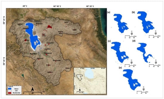
Figure 1.
ULB location (left), and the Urmia Lake levels (right) in (a) 2000, (b) 2005, (c) 2010, (d) 2015, and (e) 2020.
2.2. Data Acquisition
In this study, we used remote sensing data and a GIS spatial analysis dataset. The remote sensing data consists of Landsat satellite images with a spatial resolution of 30 m from 1990 to 2020, as presented in Table 1. As we aimed to apply a times series analysis based on the satellite image availability, we employed satellite images produced by Landsat 5 for the study years of 1990, 1995, 2000, 2005 and 2010. Accordingly, based on the availability of satellite image from Landsat 8 from 2013, we employed these data for the study years of 2015 and 2020. The selection of study years with an interval of five were based on the discussion with experts and authorities for considering the Urmia Lake drought and its respective environmental impacts. To delineate areas based on their susceptibility to soil degradation, we also employed supplementary data (Table 2) on topographic-, hydrological-, and anthropogenic factors. Geological maps at a scale of 1:25,000 were also used to derive the geological setting of the study area. The topography map at a scale of 1:25,000 was used to generate the digital elevation model (DEM) based on the spatial analysis. The DEM was then used to derive the slope, slope length, aspect, distance from rivers, drainage density, and curvature maps.

Table 1.
Landsat5/8 bands and their characteristics used to select the relevant soil salinity indices based on their spectral characteristics and signatures.
Table 2.
List and details of datasets used for soil salinity monitoring and degradation mapping.
The DEM was also used to compute the hydrology datasets of stream power index (SPI) and topographic wetness index (TWI). The SPI is estimated along the stream network to assess the change in magnitude of stream power between pre- and post-development scenarios [42]. Basically, TWI defines the effect of topography on the location and size of saturated source areas of runoff generation [43,44]. The parameter TWI has been significantly investigated for soil degradation mapping and constitutes one of the most commonly used conditioning factors [44]. The soil type, depth, and erodibility were obtained from pedology maps at a scale of 1:50,000. For the rainfall map, initial data were obtained from meteorological stations in the ULB, and the final map was computed using spatial interpolation techniques. The normalized difference vegetation index (NDVI) was derived from the Landsat satellite images. NDVI is known as an efficient index for density of vegetation covers. The land use/cover (LULC) map was derived from the Landsat satellite images obtained as part of our earlier research on monitoring the LULC changes in the ULB from 1990–2020 using an integrated approach of object-based image analysis and deep learning techniques [31,38,39]. We used 150 ground control data points and their respective laboratory analysis to validate the results. These data points and samples were obtained during fieldwork in 2020 and supplemented with historical soil salinity data from the Organization of Agriculture and Natural Resources (OANR, 2020). All data were collected in the coordinate system of Universal Transverse Mercator Zone 38 N, World Geodetic System 1984. As Table 2 shows these data we obtained from different resources. Thus, all data preparation (e.g., extraction, editing, reformation, distance computation, etc.), and standardization were carried out in Arc GIS environment.
3. Methodology
We applied an integrated approach of remote sensing image processing and GIS spatial analysis to detect the trends of environmental phenomena, specifically related to soil salinity and soil degradation in the study area. The methodology comprises two main steps, namely the soil salinity trend assessment using satellite imagery and the soil degradation mapping based on the GIS spatial analysis and multi criteria decision analysis (MCDA). We used the eight soil salinity indices including: combined spectral response index; normalized differential Salinity index; salinity index (SI 1,2,3); normalized differential infrared index and vegetation soil salinity index to carry out the soil salinity trend assessment. We aimed to determine the degree to which each of the indices influences soil salinity based on the ground control point dataset obtained through fieldwork.
Therefore, the accuracy of each index was assessed using linear regression analysis. After determining the most accurate index, we used it to compute the soil salinity trend from 1990 to 2020. In the second step, we used the GIS-MCDA method in combination with fuzzy logic to identify the areas affected by soil degradation based on the results of the soil salinity trend computed in the first step in combination with ancillary data. Figure 2 shows a flowchart for the main steps of our research methodology.
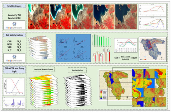
Figure 2.
Flowchart for the main schema of the research methodology. The upper and middle parts of this figure show the implementation of the time-series satellite image analysis for soil salinity monitoring and validation. The lower section shows the research methodology for a MCDA approach for soil degradation mapping.
3.1. Soil Salinization Monitoring
Earth observation satellite imagery is integral for soil salinity monitoring. The spectral reflectance characteristics of salt at the soil surface can be used to identify and monitor soil salinity [8]. Furthermore, well-organized soil management using the latest remote sensing methods and soil salinity monitoring plays an important role, especially in the preservation of arable lands [40]. We employed the eight best-known soil salinity indices to identify saline regions and compare their efficiency (Table 3). Soil salinity indices derived from the visible and near-infrared (NIR) bands of satellite images have been used in several studies to create soil salinity maps [5,8,19,45,46,47,48]. However, comparing the efficiency of soil salinity indices remains a field of interest and further studies are required to introduce, compare and apply the efficient indices.
We used Landsat time-series (1990–2020) satellite images with a spatial resolution of 30 m and seven spectral wavelength ranges [49] to ascertain the areas of bare soil, vegetation, water bodies, and exposed salt areas resulting from the Urmia Lake drought based on their spectral characteristics. We verified these resulting areas using the ground control sample points collected in the field operation. We used the spectral range of bands three to seven to distinguish between soil and salt and thus recognize soil salinity in the study area based on the spectral value of saline flow sources and farmlands, which we obtained through field measurements and laboratory analysis. This sampling data and their laboratory analysis were used for validation of results as we discussed in the next sections. The soil types with low salinity correspond to high vegetation areas that exhibit high NIR values. The red, green, blue, and short-wave infrared (SWIR) channels show different reflections for different salinity levels but with less reflectance for the NIR channel. Therefore, the NIR channel can be used to estimate salt content. Different salt thresholds may have different reflectivity curves based on the physiochemical and environmental characteristics (e.g., texture, climate), which serve as the basis for selecting the most suitable estimation model. We applied eight indices recommended by earlier studies [1,8,17,19,50] and correlated the modeled results with the wavelengths obtained from sampling points to determine the soil salinity.
Table 3.
The soil salinity indices and their respective equations used in this study.
Table 3.
The soil salinity indices and their respective equations used in this study.
| Index | Main Equation | References |
|---|---|---|
| Combined Spectral Response Index (CSRI) | (B + G)/(R + NIR) × NDVI | [51] |
| Normalized Differential Salinity Index (NDSI) | (R − NIR)/(R + NIR) | [52] |
| Salinity index (SI-T) | (R/NIR) × 100 | [53] |
| Salinity Index (SI-1) | NIR/SWIR | [54] |
| Salinity Index (SI-2) | (B − R)/(B + R) | [55] |
| Salinity Index (SI-3) | (B × R)/G | [55] |
| Normalized Differential Infrared Index (NDII) | (NIR − SWIR1)/(NIR + SWIR1) | [56] |
| Vegetation Soil Salinity Index (VSSI) | 2 × G − 5 × (R + NIR) | [56] |
3.1.1. Combined Spectral Response Index (CSRI)
This index uses the green, blue, red, and NIR bands. The CSRI can only be computed with the NDVI value, as per Equation (1) [50]:
where B is the blue band, G is the green band, R is the red band with a wavelength, and NIR is the near-infrared band with a wavelength of 0.76 to 0.90 micrometers. The NDVI can also be calculated using the following Equation (2):
According to Fernandez-Buces et al. [50], to calculate the CSRI, the combination of bands one to four and the NDVI achieve the highest accuracy. The resulting integrated algorithm is called the Combined Spectral Response Index (COSRI) and reflects the combination of spectral responses of bare soil and vegetation. We used Landsat-5 bands 1–4 to map the soil salinity for 2000, 2005 and 2010, and Landsat-8 bands 2–5 to map the soil salinity for 2015 and 2020, as presented in Table 2.
3.1.2. Normalized Differential Salinity Index (NDSI)
The NDSI index is one of the most well-known indicators in soil studies using remote sensing and has been widely applied by earlier researchers [19,21,52]. The NDSI is based on the red and infrared spectral ranges. The general form of this index is defined by Equation (3). We computed this index based on the Landsat-8/OLI bands four and five.
3.1.3. Salinity Index (SI-T)
This index was introduced by Tripathi et al. [53], in the early days of remote sensing and satellite image processing. The salinity index is based on the difference between the red (R) and near-infrared (NIR) bands multiplied by 100, as per Equation (4):
(R/NIR) × 100
3.1.4. Salinity Index (SI-1)
This index was proposed by Bannari et al. [54] and uses bands nine and ten of the advanced land imaging (EO-1) sensor. In this study, we used Landsat bands five and six to calculate the soil salinity. This index is based on the fraction between the NIR and SWIR bands, as per Equation (5), where NIR is the near-infrared band, and SWIR is the short-wave infrared band.
3.1.5. Salinity Index (SI-2) and Salinity Index (SI-3)
The salinity indexes (SI-2 and 3) are also effective for soil salinity assessment. According to Abbas and Khan [55] the visible range of spectral wavelengths is more useful for detecting soil salinity. The following Equations (6) and (7) represent how SI 2–3 are implemented, whereby R, G and B represent the red, green and the blue bands, respectively. These indexes were developed using the equivalents to bands two and four in Landsat-8/OLI, and bands one and three in Landsat-5/TM, respectively.
3.2. Normalized Differential Infrared Index (NDII)
The NDII index represents the normalized difference between the NIR and SWIR of the electromagnetic spectrum. The NIR band and the SWIR band, which correspond to bands five and six in Landsat five and eight were used to calculate this index as per Equation (8):
3.2.1. Vegetation Soil Salinity Index (VSSI)
The VSSI is applied to discriminate between soil and vegetation stress, which has been addressed by several earlier studies [56,57,58]. The index is based on the R, G and NIR bands as per Equation (9):
3.2.2. Google Earth Engine
With the recent advances in earth observation technologies, the increasing availability of data from more and more different satellite sensors, as well as progress in semi-automated and automated classification techniques, enable the (semi-) automated remote monitoring and analysis of large areas. Online platforms such as Google Earth Engine (GEE) bring data-driven techniques to the desktops of researchers while changing workflows and making excessive data downloads redundant [47]. The GEE provides free access to a wide range of global satellite images and efficient data-driven machine learning tools, making it a powerful resource for various remote sensing applications [38]. The GEE is an ideal platform for large-scale monitoring and modeling of earth’s features as a result of its various geospatial datasets, rich reusable library, and easy to use process [35]. It has been used in numerous studies for remote sensing processes using a wide range of images and spatial information such as LULC mapping, agricultural crop monitoring, natural hazard, soil salinization and among others [12,59,60]. Based on the soil salinity indexes, we used the GEE environment to compute and monitor the soil salinity ratio for 1990 to 2020.
3.2.3. Accuracy Assessment of Soil Salinity Monitoring Indices
Numerous researchers have evaluated soil salinity monitoring results using sampling points and their spectral characteristics, such as electrical conductivity [26,61,62,63]. As our aim was to compare the efficiency of eight soil salinity indices, we validated the results based on 150 ground control sample points collected during field work in 2020 and their physiochemical laboratory analysis. We also used the 300 control points from the historical soil salinity datasets collected annually in the field by the Organization of Agriculture and Natural Resources (OANR) to evaluate the accuracy of the soil salinity maps computed for 1990, 1995, 2000, 2005, 2010 and 2015. We then used 450 ground control sample points (including 150 from 2020 and 300 historical data points from 1990, 1995, 2000, 2005, 2010, and 2015) and the computed physiochemical soil characteristics, including electrical conductivity (EC), exchangeable sodium percentage, and pH, to validate the accuracy of our results. It has to be indicated that the EC is a common soil index used to express the soil salinity and its impacts on the fertility of the land and is, thus, an indicator of the suitability of the soil for growing crops [64]. Table 4 shows the physical and chemical properties measured in the ground control sample points, namely the soil texture (percentage of sand, silt, and clay particles) determined using the hydrometer method [65], the particle density [66], the percentage of organic matter [67], the calcium carbonate (CaCO3) content, the pH, and the EC in a 1:5 soil to distilled water suspension, and the sodium adsorption ratio (SAR) in saturated paste extract. We used the linear regression analysis for the accuracy assessment and to analyze the efficiency of the soil salinity indices. We used the standardization of the data obtained from the indices to compare the values obtained from the indices and the field observation data. Thus, an appropriate coefficient was determined for each index. After computing the soil salinity trend using each index and comparing the efficiency of all indices, we validated the results using the ground control sample data. We then calculated the correlation rate using linear regression. Earlier studies reported the linear regression to be an efficient correlation assessment method for soil studies [16,19]. The linear regression is calculated based on equation 10, where ‘y’ is modeled as beta1 (b1) times x, plus a constant beta0 (b0), plus an error term e.
y = b0 + b1 × x + e
Table 4.
Physiochemical laboratory analysis for saline soil sampling/ground control points for the accuracy assessment of the soil salinity maps produced by the various indices, as explained in Table 3.
3.2.4. Soil Degradation Mapping
Criteria Selection and Standardization
The soil degradation mapping is a multi-step approach that requires us to consider the interaction of the respective indicators, including climate, land use, and topography, to name a few. GIS-based MCDA can be applied to evaluate the interaction of soil degradation impacting criteria. GIS-MCDA methods support meaningful spatial decisions by integrating multiple criteria from various spatial data sources [68,69,70,71,72]. Leveraging this capability, we employed 14 criteria in four major groups to analyze soil salinity and develop a soil degradation risk map (Figure 3). The relevant criteria were selected based on previous international studies on soil degradation mapping [48,72,73,74,75,76] as well as earlier local soil research studies [16,19]. We selected criteria that represent the soil characteristics and relevant factors that impact the soil degradation in ULB. The initial list of criteria were discussed with local experts in the Department of Soil Science at the University of Tabriz and experts in the Organization of Agriculture and Natural Resources to take the physical properties of the study area into account and select the relevant criteria accordingly. The efficiency of the selected criteria was evaluated during fieldwork, which also supported our sensitivity analysis to determine the efficiency of the selected criteria. Table 5 shows the list of selected criteria for soil degradation mapping. After identifying the relevant criteria, the required geometric and topological editing was carried out to develop the criteria into a spatial dataset. In GIS-MCDA, standardization is critical due to the variety of data sources and the different measurement scales. Thus, the criteria were standardized using the pairwise comparison method [77,78,79,80], which is commonly used for rating and standardizing ordinal values. The standardization technique was also applied to scale the data for criterion weighting, sensitivity analysis, and aggregation. This was accomplished using fuzzy standardization functions. In contrast to a standard binary set, where each element must have a membership degree of either zero or one, a fuzzy set’s members can have membership degrees ranging from zero to one [81].
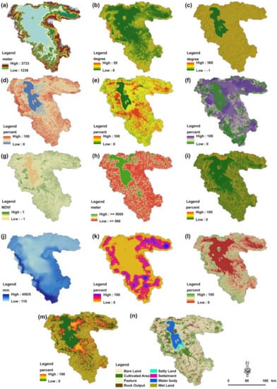
Figure 3.
Selected criteria including: (a) elevation; (b) slope degree; (c) slope aspect; (d) curvature; (e) soil depth; (f) soil texture; (g) vegetation density; (h) distance from river; (i) Stream Power Index; (j) annual precipitation; (k) drainage density; (l) slope length; (m) topographic wetness index; and (n) LULC.
Table 5.
Selected criteria, initial data sources, and mathematical representation of methods used for soil degradation mapping.
Criteria Weighting and Sensitivity Analysis
Criteria weighting is necessary to determine the significance of each indicator in decision-making [82]. We used the fuzzy analytical network process (FANP) for criteria weighting. Previous studies have confirmed the efficiency of the FANP for criteria weighting [61]. The FANP method is one of the most frequently used methods for computing the criteria’s intrinsic weights [83,84,85,86,87]. To apply the FANP, we used the initial criteria ranking obtained in the pairwise comparison matrix based on expert opinions. Therefore, 30 experts from the Organization of Agriculture and Natural Resources, the Department of Soil Research, and the University of Tabriz’s Department of Soil Sciences were asked to rank the criteria from one to nine. Then, the pairwise comparisons were carried out using Super Decision software, and the weight of each criterion was obtained, as shown in Table 6. A consistency ratio (CR) was used to determine the reliability of the computed weights as part of the FANP implementation. According to Saaty [83], the optimal CR should be >0.1, which implies that the matrix has an acceptable level of consistency and that the weighting can be used in the data aggregation. In this research, we computed the CR to be 0.04, which indicates a very acceptable level of CR.
Table 6.
The computed criteria weights from the FANP method for soil degradation mapping.
We applied the fuzzy membership command in GIS to standardize the layers. Therefore, the linear function was used to convert the classified raster layers to fuzzy standard layers, in which the pixel values ranged between zero and one. The FANP approach is a popular assessment method that combines the analytical network process method with the fuzzy level evaluation method [84,85]. Furthermore, the fuzzification allows us to quantitatively evaluate the qualitative criteria through fuzzy mathematics membership theory in complex decision-making [86]. The results of this step included 14 standardized raster maps, whereby the values of each map ranged between zero and one. Figure 4 shows the spatial distribution of the selected and standardized criteria. The ranking was determined based on the impact of each class of layers on soil degradation.
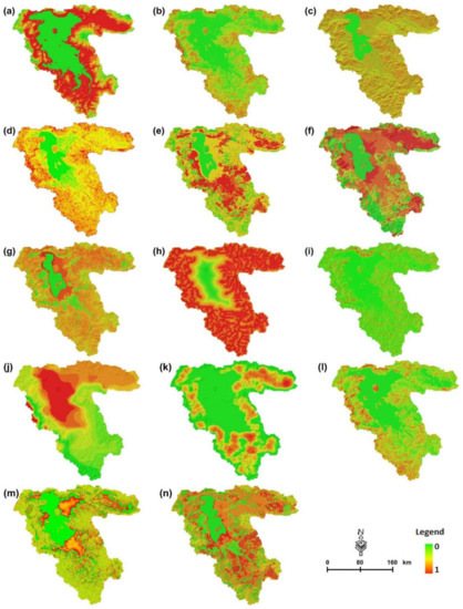
Figure 4.
Standardized soil degradation map showing: (a) elevation; (b) slope degree; (c) slope aspect; (d) curvature; (e) soil depth; (f) soil texture; (g) vegetation density; (h) distance from river; (i) Stream Power Index; (j) annual precipitation; (k) drainage density; (l) slope length; (m) topographic wetness index; and (n) LULC.
The sensitivity analysis was applied to compute the sensitivity of the weights obtained through the FANP. Technically, uncertainty in GIS-MCDA is inevitable due to the heterogeneous data sources, expert knowledge for criterion ranking, and modeling flaws [82]. In this case, the criteria weighting contributes significantly to the MCDA framework’s ambiguity. According to previous studies, such ambiguity might even lead to erroneous outcomes. To reduce the risk of error in our GIS-MCDA-based decision model, we used a sensitivity analysis to determine the uncertainty associated with the FANP’s weights for spatial modeling. To compute the uncertainty of the criteria weights, we employed an integrated approach of Monte Carlo simulation (MCS) and a global sensitivity analysis (GSA) [87].
The original FANP weights can also be used as input weights for MCS and sensitivity analysis based on the GSA approach. Thus, in our study, the implementation of MCS-GSA consists of the following four main steps: (a) obtaining training data from field work that is uniformly distributed throughout the high soil degradation areas, as discussed above; (b) using the FANP’s weights as reference weights; (c) running the MCS-based simulation 10,000 times; and (d) computing the spatial distribution of ranks (minimum, maximum, average and standard deviation) results using inverse weighted distance spatial interpolation techniques (Figure 5). Table 6 shows the considered criteria, the obtained FANP weights as references weights, and the results of the GSA for sensitivity analysis. The difference of S and St is not very significant, which indicates that the obtained FANP weights can be used in the data aggregation. The GSA method also allows us to compute the two critical indexes of S (first-order) and St (total effect). Technically, the S and St represent the FANP’s weights indicated in a semantic manner. In this context, any difference between the value and order of the S and St indexes and the reference weights (e.g., FANP’s weights) can be considered as the uncertainty associated with the criteria weights. A significant difference in the S and St indicates the level of uncertainty in the reference weights (e.g., FANP) and may result in inaccurate results.
Figure 5.
Results of MCS-based criteria weight sensitivity analysis, including: (a) computed maximum rank, (b) average rank, and (c) standard deviation. These maps are based on the MCS sensitivity analysis of the computed criteria weights.
Spatial Aggregation and Validation
The final maps were developed using the spatial data aggregation of the specified criteria based on the computed weights. The geographical criterion from one map layer are combined with the attribute (numerical) properties of the other criterion in this numerical technique. The soil degradation mapping was carried out based on the ordered weighted average (OWA). The OWA is a prominent spatial aggregation approach in GIS and has been validated by numerous previous studies [47,78,79,80,81]. OWA employs fuzzy decision rules to model the linguistically as effective spatial aggregation. OWA provides a parameterized class of multi-criteria aggregating operators between the minimum and maximum. Technically, the OWA employs fuzzy decision rules for modeling the linguistically as effective spatial aggregation. In our study, the computed FANP’s weights were used as reference weights of OWA to produce the soil degradation map for the ULB. We then validated the results. Therefore, we used the relationship between the soil salinity ratio of 150 sampling ground control points from 2020 and their physiochemical laboratory analysis results, as represented in Table 4.
4. Results
4.1. Soil Salinity Monitoring
The soil salinity monitoring results based on the satellite images of 2020 and the remote sensing indexes are represented in Figure 6. Due to the large number of figures generated in this study, we only include the results of 2020 in this paper, but the results obtained for the early study years (1990–2015) were used for the soil salinity monitoring and trend assessment. As Figure 6 shows, different results might be obtained by applying different soil salinity indices. We applied the accuracy assessment based on the soil salinity ratio of 450 ground control sample points collected during field work and their physiochemical analysis (Table 4) to determine the accuracy of the results. Figure 7 shows the results of the correlation between the ground control sample points and the soil salinity indices. The results revealed that the CSRI index, with a correlation of 0.95, and the SI-1 index, with a correlation of 0.83, yielded the best results of the examined soil salinity indices. It should be noted that other indices also performed adequately in soil salinity detection, as represented in Figure 8. However, as one of the main objectives of this research was to investigate the most efficient soil salinity index, the next step was to use the time-series satellite images from 1990–2020 to derive the soil salinity map for the ULB.
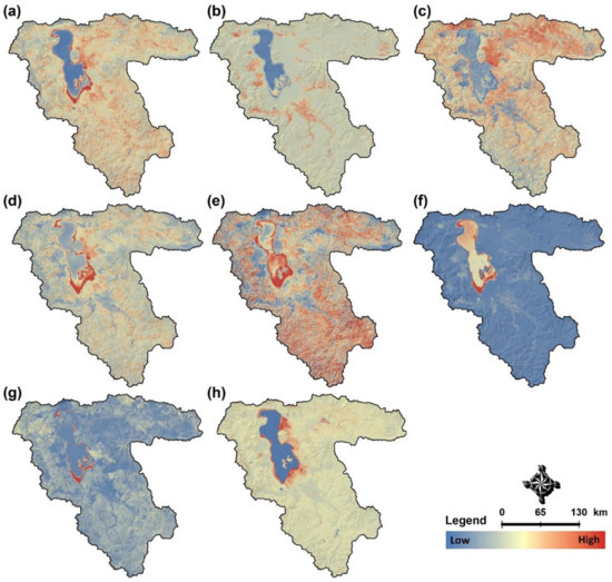
Figure 6.
The soil salinity monitoring indices applied to the satellite images of 2020 using the different soil salinity indexes of (a) CSRI, (b) NDSI, (c) VSSI, (d) SI-T, (e) SI-1, (f) SI-2, (g) SI-3, and (h) NDII, whereby red indicates areas with high soil salinity. Due to the large number of maps generated in this research, we only show the results of soil salinity indices for 2020.
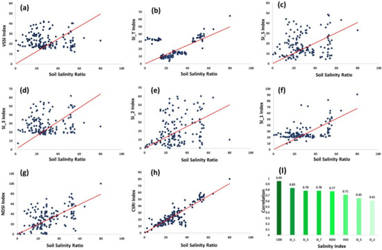
Figure 7.
Validation results of the correlation between the soil salinity indices (see Figure 6) and the soil salinity data obtained in the laboratory for the ground control points (see Table 4). The computed correlations show the results for soil salinity indices: (a) VSSI; (b) SI_T; (c) SI_5; (d) SI_3; (e) SI_2; (f) SI_1; (g) NDSI; (h) CSRI; and (I) comparing the accuracy of all indices. The CSRI achieved the highest accuracy.
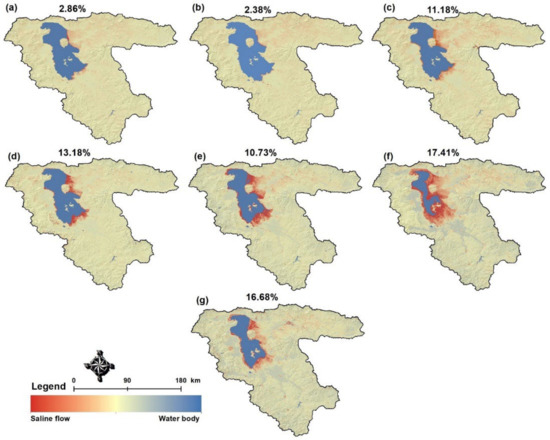
Figure 8.
Soil salinity based on the CSRI index in: (a) 1990; (b) 1995; (c) 2000; (d) 2005; (e) 2010; (f) 2015; and (g) 2020. As can be seen on the maps, the soil salinity (red areas) has increased significantly from 1990 to 2020.
Figure 8 shows the results of the time-series soil salinity monitoring in the ULB. Based on these results, there is a significant correlation between the lake drought and the expansion of soil salinity in the vicinity of the lake. The results also revealed that the soil salinity and expansion of salty lands were limited to the areas adjacent to the lake. As shown in Figure 8, the soil salinity started becoming noticeable from 2000 and increased slightly between 2000 and 2005. Then, there was a considerable increase from 2005 to 2010. Figure 8f shows that there was intensive soil salinity in the vicinity of the lake when Urmia Lake experienced a severe drought in 2015. As a result of the increase in annual precipitation from 2018 to 2020 and restoration efforts in some parts of the lake, the soil salinity has also reduced accordingly. Using the CSRI index, we were able to identify the trend of soil salinity changes in the ULB. According to the results of the CSRI index, the soil salinity changes reflected an increase of 2.86% in 1990, 2.38% in 1995, 11.18% in 2000, 13.18% in 2005, 10.73% in 2010, 17.41% in 2015, and 16.68% in 2020. To examine the accuracy of the CSRI index results, we also employed the computed soil salinity ratio of ground control sample data for 2020 as well as the historical ground control soil salinity dataset, as discussed in the accuracy assessment section. Figure 9 depicts the results of the validation of the CSRI index from 1990–2020.
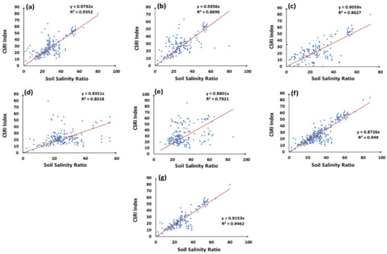
Figure 9.
Validation results of CSRI index (see Figure 8) based on the ground control sample points obtained during field work and based on the historical soil salinity dataset (see Table 4). The charts indicate that valid soil salinity maps have been developed for: (a) 1990, (b) 1995, (c) 2000, (d) 2005, (e) 2010, (f) 2015, and (g) 2020.
4.2. Soil Degradation Mapping
We applied a GIS spatial analysis to develop the soil degradation map. We used the soil salinity index proposed by Szabolcs [86], to classify the results into soil degradation risk categories. According to this index, electrical conductivity (EC) < 4 represents no salinity, 4–8 indicates low salinity, 8–16 medium salinity, 16–32 high salinity, and 32 < stands for very high salinity. Thus, the land degradation risk map is classified into five categories from no risk to very high risk using the GIS analysis, as represented in Figure 10. According to the resulting map, 12.49% of the area has a very high risk, 25.96% has a high risk, and the rest of the study area has a moderate and lower than moderate risk of soil degradation (Table 7). We validated the results to confirm their accuracy using the ground control sample points obtained in 2020 (Table 4). Table 8 gives the results of the validation matrix, which is based on the computed EC of ground control sample points. The results of the validation show that the overall accuracy of the calculations is 94.44%, and the kappa coefficient is 91.69%. This accuracy indicates the reliability of the results. To clearly understand which areas are affected by soil degradation risk, magnified views of its main centers are shown in Figure 11.
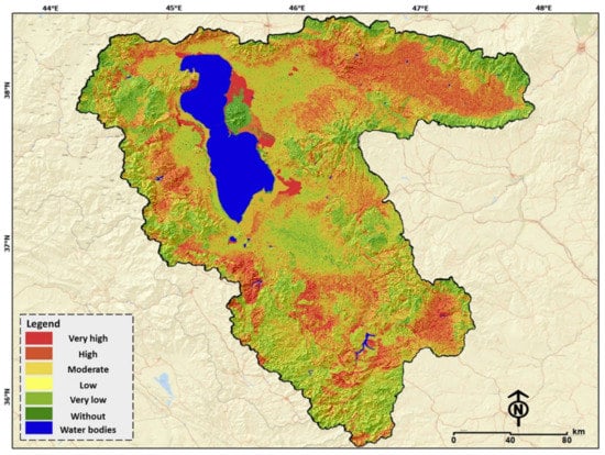
Table 7.
Percentage of soil degradation areas in ULB computed from the soil degradation risk map presented in Figure 10.
Table 8.
Field observation data matrix (soil electrical conductivity) based on the ground control sample points and computed EC.
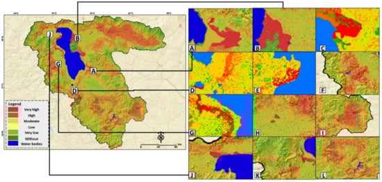
Figure 11.
Enlarged views of regions affected by soil degradation risk to show details of the spatial variation of the soil degradation risk in the study area (A,B,D,G,J) are located around Urmia Lake and are severely affected by Urmia Lake salts).
5. Discussion
The results of the time-series analysis for soil salinity monitoring indicated that the lake drought and associated exposed salt lands significantly affected the soil salinization in the plains in the vicinity of the lake. According to the results, the lake drought has significantly impacted soil salinization, with saline areas having increased from 2.86% in 1990 to 17.41% in 2015. Such intensive soil salinity has significant impacts on the environment and the productivity of the farmlands. One of the primary tangible aspects of this salinization can be observed in the increase in the EC of soils in farmlands. Soils with an EC of more than 4 ds/m can be considered saline soils that might threaten the productivity of the farmlands. Table 9 shows the effect of increasing EC values on the fertility and productivity of soils based on the Szabolcs scale [86]. According to the results of the time-series soil salinity monitoring, the EC of farmlands in ULB has been increasing significantly, which is causing challenges for agriculture as it affects the productivity and fertility of this area and can lead to food production shortages.
Table 9.
Classification of soils based on their salinity [86].
The increasing availability of a wide range of earth observation products with improved spatial and spectral information demands the development of new and efficient methods for soil salinity monitoring. Due to the extensive costs and limitations associated with field-based soil salinity assessments, most studies, both at regional and global scales, rely on soil degradation data from risk maps, expert opinions and estimations, and computations obtained from empirical models [87,88]. Thus, researchers began optimizing soil salinity indices and improving their accuracy. In this context, Xiaoyan et al. [4] applied several soil salinity indices (such as the principal component regression, multiple linear regression, and partial least squares regression) and compared their efficiency. Zhang et al. [74] employed the vegetation index (NDVI) and soil salinity index based on the original band of Landsat 7 satellite images to improve the effectiveness of salt monitoring techniques. Allbed et al. [11] reported NDSI and SI_T as the best indices for soil salinity assessments. According to our results, some inherent uncertainty remains in every soil salinity index, which must be overcome to obtain accurate results. However, in the context of soil salinity monitoring indices from remote sensing images, we must consider that the soil characteristics are related to multiple indicators (parent material, vegetation, and moisture) that must be taken into account when mapping soil salinity, which is also acknowledged in earlier studies [4,19,22].
In this study, we examined eight soil salinity indices to identify the most efficient method. Based on our results, the CSRI index, with a correlation of 0.95, was the most efficient soil salinity detection method. The SI-1 index, with a correlation of 0.83, was the second-most effective technique, while the SI-5 and SI-2, with correlation values of 0.65 and 0.61, yielded lower accuracies. Technically, soil salinity influences not only the reflectance of the soil but also the degree of surface looseness, water quality, and aboveground plant growth. As a result, the quantitative inversion of the salt content may be obtained in soil salinity studies by integrating the vegetation index, water index, and soil index [89,90]. Thus, any efficient soil salinity assessment methods should be optimized based on the local soil characteristics. In addition, in most cases, the developed indices must be optimized and customized based on the local characteristics, as pointed out in earlier studies [21,45].
As indicated above, various criteria impact the soil characteristics and must be considered when modeling the soil properties. The results of this research indicated that GIS-MCDA can be used to analyze the various criteria impacting the soil degradation risk in ULB, and can thus be used for soil degradation risk analysis. According to the results of various investigations, soil salinity is one of the manifestations of soil degradation that directly reduces agricultural productivity and causes other environmental irregularities. Therefore, we examined the criteria affecting land degradation using 14 criteria in four categories, as presented in Table 5. The detailed results revealed that 38.46% of the study area has a very high or high risk of degradation. This means that these affected areas in the province are unfavorable for agriculture production. Based on the decreasing lake level of Urmia Lake and the emergence of salt diffusion centers, it is expected that the percentage of soil salinity will continue to increase in the future.
6. Conclusions
In this research, we identified areas affected by soil salinity using remote sensing indices and satellite images. Then, we applied the soil degradation risk analysis using the GIS-MCDA spatial modelling. Based on the results, we propose the regular monitoring of areas affected by soil salinization and degradation, the development of new methods, and their implementation in the online platforms and advanced cloud computing technologies such as GEE, to support decision-makers and authorities with up-to-date and near real-time monitoring of the soil salinity in the region. Applying several soil salinity indices indicated that selecting a beneficial technique might be challenging due to the similarity of methods. However, results might be different and accurate data is required for accuracy assessment. The use of state-of-the-art methods and technologies is the key to obtaining highly accurate results using remote sensing. Therefore, the development of suitable algorithms, together with the right indices and high-resolution satellite images, is critical to detect salinity centers with high accuracy.
Our results show that the Urmia Lake drought and the associated occurrence of salt diffusion centers and extensive soil salinity indirectly impact agriculture activities. The ULB, with about 360,000 hectares of croplands and 140,000 hectares of orchards, makes up about 8.5% of Iran’s farmlands and significantly contributes to food production. The ULB is also home to 7.3 million people living in 63 cities and 520 villages, all of which are threatened by the intensive environmental impacts of the hyper-saline lake drought. The UNEP recognized Urmia Lake as a worrying case, which clearly shows the need for immediate restoration initiatives. Therefore, the results of this research shall be used by authorities and environmental planners to identify potential constraints and prevent soil misuse and vegetation destruction. These results will lead to the observation of soil salinization and degradation, thus helping to reduce the rural exodus to the cities located in the ULB, which is causing further challenges for these cities. Our results will also provide key information for decision-makers and support them in the sustainable development of northwest Iran. Due to the lack of suitable environmental management and agricultural practices, the drying rate of Urmia Lake has increased. The subsequent soil salinization has expanded, which is threatening the fertility of the soils in the vicinity of the lake. This has become a critical concern in northwest Iran and neighboring countries such as Turkey, Azerbaijan, Iraq, and Armani as this phenomenon impacts all hyper-saline lakes.
Author Contributions
Conceptualization, B.F. and D.O.; methodology, B.F.; software, K.M.A.; validation, D.O., M.M. and K.M.A.; formal analysis, K.M.A.; investigation, D.O.; resources, K.M.A.; data curation, D.O.; writing—original draft preparation, B.F.; writing—review and editing, T.B.; visualization, M.M.; supervision, B.F.; project administration, B.F.; funding acquisition, B.F. All authors have read and agreed to the published version of the manuscript.
Funding
This research was jointly funded by a research grant from the University of Tabriz (s818) and the Alexander von Humboldt Foundation.
Data Availability Statement
The research data might be available by request to the corresponding author.
Acknowledgments
The authors thank the anonymous reviewers for their constructive comments and suggestions on the earlier versions of this article, which significantly supported us in improving the manuscript. We would like to thank Tobia lakes in the GIScience Department of the Humboldt Humboldt-Universität zu Berlin for the constructive feedback on the earlier version of this article. We also thank the Organization of Agriculture and Natural Resources for providing ground control sample point data as well as the historical soil salinity dataset.
Conflicts of Interest
The authors declare no conflict of interest.
References
- Kopittkea, P.M.; Menziesa, N.W.; Wangb, P.; Brigid, A.; McKennaa, B.A. Soil and the intensification of agriculture for global food security. Environ. Int. 2019, 132, 105078. [Google Scholar] [CrossRef] [PubMed]
- Vengosh, V. Salinization and Saline Environments. Treatise Geochem. 2003, 9, 612. [Google Scholar]
- Abbasi, G.H.; Akhtar, J.; Ahmad, R.; Jamil, M.; Anwar-ul-Haq, M.; Ali, S.; Ijaz, M. Potassium application mitigates salt stress differentially at different growth stages in tolerant and sensitive maize hybrids. Plant Growth Regul. 2015, 76, 111–125. [Google Scholar] [CrossRef]
- Xiaoyan, S.; Jianghui, S.; Haijiang, W.; Xin, L. Monitoring soil salinization in Manas River Basin, Northwestern China based on multi-spectral index group. Eur. J. Remote Sens. 2021, 54, 176–188. [Google Scholar]
- Gorji, T.; Yildirim, A.; Hamzehpour, N.; Tanik, A.; Sertel, E. Soil salinity analysis of Urmia Lake Basin using Landsat-8 OLI and Sentinel-2A based spectral indices and electrical conductivity measurements. Ecol. Indic. 2020, 112, 106173. [Google Scholar] [CrossRef]
- OECD Glossary. Glossary for Statistical Terms. 2001. Available online: https://stats.oecd.org/glossary/about.asp (accessed on 1 October 2001).
- Zovkoa, M.; Romića, D.; Colombo, C.; Di Ioriob, E.; Romića, M.; Buttafuococ, G.; Castrignanò, A. A geostatistical Vis-NIR spectroscopy index to assess the incipient soil salinization in the Neretva River valley, Croatia. Geoderma 2018, 332, 60–72. [Google Scholar] [CrossRef]
- Zarei, A.; Hasanlou, M.; Mahdianpari, M. A comparison of machine learning models for soil salinity estimation using multi spectral earth observation data, ISPRS Annals of the Photogrammetry. Remote Sens. Spat. Inf. Sci. 2021, 3, 257–263. [Google Scholar]
- Gontia-Mishra, I.; Sasidharan, S.; Tiwari, S. Recent developments in use of 1-aminocyclopropane-1-carboxylate (ACC) deaminase for conferring tolerance to biotic and abiotic stress”. Biotechnol. Lett. 2014, 36, 889–898. [Google Scholar] [CrossRef]
- Kamran, M.; Parveen, A.; Ahmar, S.; Malik, Z.; Hussain, S.; Sohaib Chattha, M.; Hamzah Saleem, M.; Adil, M.; Heidari, P.; Chen, J.T. An Overview of Hazardous Impacts of Soil Salinity in Crops, Tolerance Mechanisms, and Amelioration through Selenium Supplementation. Int. J. Mol. Sci. 2020, 21, 148. [Google Scholar] [CrossRef]
- Allbed, A.; Kumar, L.; Aldakheel, Y.Y. Assessing soil salinity using soil salinity and vegetation indices derived from IKONOS high-spatial resolution imageries: Applications in a date palm dominated region. Geoderma 2014, 230, 1–8. [Google Scholar] [CrossRef]
- Sinha, D.N.; Singh, A.N.; Singh, U.S. Site Suitability Analysis for Dissemination of Salt Tolerant Rice Varieties in Southern Bangladesh. In Proceedings of the ISPRS Technical Commission VIII Symposium, Hyderabad, India, 9–12 December 2014; The International Archives of the Photogrammetry, Remote Sensing and Spatial Information Sciences. Volume 8. [Google Scholar]
- Sidike, A.; Zhaom, S.; Wen, Y. Estimating soil salinity in Pingluo County of China using Quick Bird data and soil reflectance spectra. Int. J. Appl. Earth Obs. Geoinf. 2014, 26, 156–175. [Google Scholar]
- Tehrany, M.S.; Shabani, F.; Javier, D.N.; Kumar, L. Soil erosion susceptibility mapping for current and 2100 climate conditions using evidential belief function and frequency ratio. Geomat. Nat. Hazards Risk 2014, 8, 1695–1714. [Google Scholar] [CrossRef]
- Agarwal, D.; Tongaria, K.; Pathak, S.; Ohri, A.; Jha, M. Soil Erosion Mapping of Watershed in Mirzapur District Using RUSLE Model in GIS Environment. Int. J. Stud. Res. Technol. Manag. 2016, 4, 56–63. [Google Scholar] [CrossRef]
- Shahbazi, F.; McBratney, A.; Maloneb, B.; Oustana, S.; Minasny, B. Retrospective monitoring of the spatial variability of crystalline iron in soils of the east shore of Urmia Lake, Iran using remotely sensed data and digital maps. Geoderma 2019, 337, 1196–1207. [Google Scholar] [CrossRef]
- Mukhopadhyay, R.; Sarkar, B.; Jat, H.S.; Sharma, P.C.; Bolan, N.S. Soil salinity under climate change: Challenges for sustainable agriculture and food security. J. Environ. Manag. 2020, 280, 111736. [Google Scholar] [CrossRef]
- Feizizadeh, B.; Kazamei Garajeh, M.; Blaschke, T.; Lakes, T. A deep learning convolutional neural network algorithm for detecting saline flow sources and mapping the environmental impacts of the Urmia Lake drought in Iran. Catena 2021, 207, 105585. [Google Scholar] [CrossRef]
- Omrani, M.; Shahbazi, F.; Feizizadeh, B.; Oustan, S.; Najfai, N. Application of remote sensing indices to digital soil salt composition and ionic strength mapping in the east shore of Urmia Lake, Iran. Remote Sens. Appl. Soc. Environ. 2021, 22, 100498. [Google Scholar] [CrossRef]
- Thaker, N.P.; Brahmbatt, N.; Shah, K. Review impact of soil salinity on ecological, agriculture and socioeconomic concerns. Int. J. Adv. Res. 2021, 9, 979–986. [Google Scholar] [CrossRef]
- Abdel, L.A. Changes of antioxidative enzymes in salinity tolerance among different wheat cultivars. Cereal Res. Commun. 2010, 38, 43–55. [Google Scholar] [CrossRef]
- Najafi, P.; Navid, H.; Feizizadeh, B.; Blaschke, T. Fuzzy Object-Based Image Analysis Methods Using Sentinel-2A and Landsat-8 Data to Map and Characterize Soil Surface Residue. Remote Sens. 2019, 11, 2583. [Google Scholar] [CrossRef]
- Utuk, I.O.; Ekongm, E.D. Land Degradation: A Threat to Food Security: A Global Assessment. J. Environ. Earth Sci. 2015, 5, 13–22. [Google Scholar]
- Scanes, C.G. Impact of Agricultural Animals on the Environment. In Animals and Human Society; Academic Press: New York, NY, USA, 2018; pp. 427–449. [Google Scholar] [CrossRef]
- Patterson, L.A.; Lutz, B.; Doyle, M.W. Climate and direct human contributions to changes in mean annual streamflow in the South Atlantic, USA. Water Resour. Res. 2013, 49, 7278–7291. [Google Scholar] [CrossRef]
- Corwin, D.L.; Yemoto, K. Salinity: Electrical conductivity and total dissolved solids. Soil Sci. Soc. Am. J. 2020, 84, 1442–1461. [Google Scholar] [CrossRef]
- Iestyn Woolway, R.; Kraemer, B.M.; Lenters, J.D.; Merchant, C.; O’Reilly, C.M.; Sharma, S. Global lake responses to climate change. Nat. Rev. Earth Environ. 2020, 1, 388–403. [Google Scholar] [CrossRef]
- Abbasian, M.S.; RezaNajafi, M.; Abrishamchi, A. Increasing risk of meteorological drought in the Lake Urmia basin under climate change: Introducing the precipitation–temperature deciles index. J. Hydrol. 2021, 592, 125586. [Google Scholar] [CrossRef]
- Anbari, M.J.; Zargami, M.; Nadiri, A. An uncertain agent-based model for socio-ecological simulation of groundwater use in irrigation: A case study of Lake Urmia Basin, Iran. Agric. Water Manag. 2021, 249, 106796. [Google Scholar] [CrossRef]
- Hemmati, M.; Ahmadi, H.; Ahmad Hamidi, S.; Naderkhanloo, V. Environmental effects of the causeway on water and salinity balance in Lake Urmia. Reg. Stud. Mar. Sci. 2021, 44, 101756. [Google Scholar] [CrossRef]
- Feizizadeh, B.; Mohmmadzadeh Alajujeh, K.; Lakes, T.; Blaschke, T.; Omarzadeh, D. A comparative approach of integrated fuzzy object-based deep learning and machine learning techniques for monitoring land use/cover changes and environmental impacts assessment. GISci. Remote Sens. 2021, 58, 1543–1570. [Google Scholar] [CrossRef]
- Mardi, A.H.; Khaghani, A.; MacDonald, A.B.; Nguyen, P.; Karimi, N.; Heidary, P.; Karimi, N.; Saemian, P.; Sehatkashani, S.; Tajrishy, M.; et al. The lake Urmia environmental disaster in Iran: A look at aerosol pollution. Sci. Total Environ. 2018, 633, 42–49. [Google Scholar] [CrossRef]
- Chakherlou, S.; Jafarzadeh, A.A.; Ahmadi, A.; Feizizadeh, B.; Shahbazi, F.; Darvishi Boloorani, A.; Mirzaei, S. Soil wind erodibility and erosion estimation using Landsat satellite imagery and multiple-criteria decision analysis in Urmia Lake Region, Iran. Arid Land Res. Manag. 2022, 1–21. [Google Scholar] [CrossRef]
- Sepuru, T.K.; Dube, T. An appraisal on the progress of remote sensing applications in soil erosion mapping and monitoring. Remote Sens. Appl. Soc. Environ. 2018, 9, 1–9. [Google Scholar] [CrossRef]
- Peng, J.; Biswas, A.; Jiang, Q.; Zhao, R.; Hu, J.; Hu, B.; Shi, Z. Estimating soil salinity from remote sensing and terrain data in southern Xinjiang Province, China. Geoderma 2019, 337, 1309–1349. [Google Scholar] [CrossRef]
- Huang, H.; Li, Z.; Huichun, Y.; Zhang, S.; Zhuo, Z.; Xing, A.; Huang, Y. Mapping Soil Electrical Conductivity Using Ordinary Kriging Combined with Back-propagation Network. Chin. Geogr. Sci. 2019, 2992, 270–282. [Google Scholar] [CrossRef]
- Zhao, W.; Persello, C.; Stein, A. Building outline delineation: From aerial images to polygons with an improved end-to-end learning framework. ISPRS J. Photogramm. Remote Sens. 2021, 175, 119–131. [Google Scholar] [CrossRef]
- Feizizadeh, B.; Gheshlaghi, H.A.; Bui, D.T. An integrated approach of GIS and hybrid intelligence techniques applied for flood risk modeling. J. Environ. Plan. Manag. 2020, 64, 485–516. [Google Scholar] [CrossRef]
- Taghadosi, M.M.; Hasanlou, M. Developing geographic weighted regression (GWR) technique for monitoring soil salinity using Sentinel-2 multispectral imagery. Environ. Earth Sci. 2021, 80, 75. [Google Scholar] [CrossRef]
- Feizizadeh, B.; Lakes, T.; Omarzadeh, D.; Sharifi, A.; Blaschke, T.; Karmizadeh, S.M. Scenario-based analysis of the impacts of lake drying on food production in the Lake Urmia Basin of Northern Iran. Nat. Sci. Rep. 2022, 12, 6237. [Google Scholar] [CrossRef]
- Feizizadeh, B.; Abdollahi, Z.; Shokati, B.; Lakes, T. A GIS-based spatiotemporal impact assessment of droughts in the hyper-saline Urmia Lake Basin on the hydro-geochemical quality of nearby aquifers. Remote Sens. 2022, 14, 2516. [Google Scholar] [CrossRef]
- Ghunowa, K.; MacVicar, B.; Ashmore, P. Stream Power Index for Networks (SPIN) Tool for Erosion Risk Assessment. In AGU Fall Meeting Abstracts; American Geophysical Union: San Francisco, CA, USA, 2019; Available online: https://ui.adsabs.harvard.edu/abs/2019AGUFMEP22B..17G (accessed on 3 June 2022).
- Gokceoglu, C.; Sonmez, H.; Nefeslioglu, H.A.; Duman, T.Y.; Can, T. The 17 March 2005 Kuzulu landslide (Sivas, Turkey) and landslide-susceptibility map of its near vicinity. Eng. Geol. 2005, 81, 65–83. [Google Scholar] [CrossRef]
- Sevgen, E.; Kocaman, S.; Nefeslioglu, H.A.; Gokceoglu, C. A Novel Performance Assessment Approach using Photogrammetric Techniques for Landslide Susceptibility Mapping with Logistic Regression, ANN and Random Forest. Sensors 2019, 19, 3940. [Google Scholar] [CrossRef]
- Zhang, Q.; Li, L.; Sun, R.; Zhu, D.; Zhang, C.; Chen, Q. Retrieval of the Soil Salinity From Sentinel-1 Dual Polarized SAR Data Based on Deep Neural Network Regression. IEEE Geosci. Remote Sens. Lett. 2020, 19, 1–5. [Google Scholar] [CrossRef]
- Najafi, P.; Feizizadeh, B.; Navid, H. A Comparative Approach of Fuzzy Object Based Image Analysis and Machine Learning Techniques Which Are Applied to Crop Residue Cover Mapping by Using Sentinel-2 Satellite and UAV Imagery. Remote Sens. 2021, 13, 937. [Google Scholar] [CrossRef]
- Feizizadeh, B.; Omarzadeh, D.; Kazamei Garajeh, M.; Lakes, T.; Blaschke, T.; Omarzadeh, D. Machine learning data-driven approaches for land use/cover mapping and trend analysis using Google Earth Engine. J. Environ. Plan. Manag. 2021, 1–33. [Google Scholar] [CrossRef]
- Afrasinei, G.M.; Melis, M.T.; Buttau, C.; Bradd, J.M.; Arras, C.; Ghiglieri, G. Assessment of remote sensing-based classification methods for change detection of salt-affected areas (Biskra area, Algeria). J. Appl. Remote Sens. 2017, 11, 016025. [Google Scholar] [CrossRef]
- Rahmati, O.; Tahmasebipour, N.; Haghizadeh, A.; Pourghasemi, H.R.; Feizizadeh, B. Evaluating the influence of geo-environmental factors on gully erosion in a semi-arid region of Iran: An integrated framework. Sci. Total Environ. 2017, 579, 913–927. [Google Scholar] [CrossRef]
- Waqasa, M.M.; Niaza, Y.; Alib, S.; Ahmadc, I.; Fahadd, M.; Rashide, H.; Awanf, U.K. Soil salonity mapping using satelite remote sensing. A case study of lowver chenab cahal system Pnjab. Earth Sci. Pak. 2020, 4, 7–9. [Google Scholar] [CrossRef]
- Fernández-Buces, N.; Siebe, C.; Cram, S.; Palacio, J.L. Palacio, Mapping soil salinity using a combined spectral response index for bare soil and vegetation: A case study in the former lake Texcoco, Mexico. J. Arid. Environ. 2006, 65, 644–667. [Google Scholar] [CrossRef]
- Khan, M.N.; Sato, Y. Monitoring hydro-salinity status and its impact in irrigated semi-arid areas using IRS-1B LISS-II data. Asian J. Geoinform. 2001, 1, 63–73. [Google Scholar]
- Deng, Y.; Wu, C.; Li, M.; Chen, R. RNDSI: A ratio normalized difference soil index for remote sensing of urban/suburban environments. Int. J. Appl. Earth Obs. Geoinform. 2015, 39, 40–48. [Google Scholar] [CrossRef]
- Tripathi, N.K.; Rai, B.K.; Dwivedi, P. Spatial modeling of soil alkalinity in GIS environment using IRS data. In Proceedings of the 18th Asian Conference on Remote Sensing, Kuala Lumpur, Malaysia, 20–24 October 1997; pp. 81–86. [Google Scholar]
- Bannari, A.; Guedon, A.M.; El-Harti, A.; Cherkaoui, F.Z.; El-Ghmari, A. Characterization of slightly and moderately saline and sodic soils in irrigated agricultural land using simulated data of advanced land imaging (EO-1) sensor. Commun. Soil Sci. Plant Anal. 2008, 39, 2795–2811. [Google Scholar] [CrossRef]
- Khan, S.; Abbas, A. Using Remote Sensing Techniques for Appraisal of Irrigated Soil Salinity. In Proceedings of the Land, Water & Environmental Management: Integrated Systems for Sustainability, Christchurch, New Zealand, 10–13 December 2007; pp. 2632–2638. [Google Scholar]
- Dehni, A.; Lounis, M. Remote sensing techniques for salt affected soil mapping: Application to the Oran region of Algeria. Procedia Eng. 2012, 33, 188–198. [Google Scholar] [CrossRef]
- Uossef, G.A.; Akbari, M.; Hassanoghli, A.; Younesi, M. Monitoring Soil Salinity and Vegetation Using Multispectral Remote Sensing Data in Interceptor Drain of Salt Marsh in Qazvin Plain. Geogr. Environ. Sustain. 2020, 10, 37–52. [Google Scholar] [CrossRef]
- Yahiaoui, I.; Bradaï, A.; Douaoui, A.; Abdennour, M.A. Performance of random forest and buffer analysis of Sentinel-2 data for modelling soil salinity in the Lower-Cheliff plain (Algeria). Int. J. Remote Sens. 2020, 42, 128–151. [Google Scholar] [CrossRef]
- Gorelick, N.; Hancher, M.; Dixon, M.; Ilyushchenko, S.; Thau, D.; Moore, R. Google Earth Engine: Planetary-scale geospatial analysis for everyone. Remote Sens. Environ. 2017, 202, 18–27. [Google Scholar] [CrossRef]
- Paz, A.M.; Castanheira, N.; Farzamian, M.; Paz, M.C.; Gonçalves, M.C.; Santos FA, M.; Triantafilis, J. Prediction of soil salinity and sodicity using electromagnetic conductivity imaging. Geoderma 2020, 361, 114086. [Google Scholar] [CrossRef]
- Hossain, M.S.; Rahman, G.M.; Solaiman, A.R.M.; Alam, M.S.; Rahman, M.M.; Mia, M.B. Estimating Electrical Conductivity for Soil Salinity Monitoring Using Various Soil-Water Ratios Depending on Soil Texture. Commun. Soil Sci. Plant Anal. 2020, 51, 635–644. [Google Scholar] [CrossRef]
- Farzamian, M.; Paz, M.C.; Paz, A.M.; Castanheira, N.L.; Gonçalves, M.C.; Monteiro Santos, F.A.; Triantafilis, J. Mapping soil salinity using electromagnetic conductivity imaging—A comparison of regional and location-specific calibrations. Land Degrad. Dev. 2019, 30, 1393–1406. [Google Scholar] [CrossRef]
- Zaman, M.; Shabbir, A.S.; Heng, L. Guideline for Salinity Assessment, Mitigation and Adaptation Using Nuclear and Related Techniques; Springer: Gewerbestrasse, Switzerland; Cham, Switzerland, 2018; Volume 2, ISBN 978-3-319-96189-7. [Google Scholar] [CrossRef]
- Gee, G.W.; Or, D. Particle Size Analysis. In Methods of Soil Analysis; Part 4. Physical Methods; Jacob, H.D., Topp, G.C., Eds.; John Wiley & Sons, Inc.: New York, NY, USA, 2002; Volume 4, pp. 201–414. [Google Scholar]
- Feizizadeh, B.; Kazamei, M.; Blaschke, T.; Lakes, T. An object based image analysis applied for volcanic and glacial landforms mapping in Sahand Mountain, Iran. Catena 2021, 198, 105073. [Google Scholar] [CrossRef]
- Nelson, D.W.; Sommers, L.E. Total Carbon, Organic Carbon and Organic Matter. In Methods of Soil Analyses; Part 3. Chemical Methods; Sparks, D.L., Ed.; SSSA: Madison, WI, USA, 1996; pp. 961–1010. [Google Scholar]
- Omarzadeh, D.; Pourmoradian, S.; Fezizadeh, B.; Khalagei, H.; Sharifi, A.; Valizadeh Kamran, K. A GIS-based multiple ecotourism sustainability assessment of West Azerbaijan province, Iran. J. Environ. Plan. Manag. 2021, 65, 490–513. [Google Scholar] [CrossRef]
- Ghaffarian, S.; Rezaie Farhadabad, A.; Kerle, N. Post-Disaster Recovery Monitoring with Google Earth Engine. Appl. Sci. 2020, 10, 4574. [Google Scholar] [CrossRef]
- Feizizadeh, B.; Omarzadeh, D.; Sharifi, A.; Rahmani, A.; Lakes, T.; Blaschke, T. A GIS-based spatiotemporal analysis of COVID-19 impacts on the urban traffic accident hotspots and transport network sustainability assessment in Tabriz. Sustanbility 2022, 14, 7468. [Google Scholar] [CrossRef]
- Abedi Gheshlaghi, H.; Feizizadeh, B.; Blaschke, T.; Lakes, T.; Tajbar, S. Forest fire susceptibility modeling using hybrid approaches. Trans. GIS 2020, 25, 311–333. [Google Scholar] [CrossRef]
- Senouci, R.; Taibi, N.-E.; Teodoro, A.; Duarte, L.; Mansour, H.; Meddah, R. GIS-Based Expert Knowledge for Landslide Susceptibility Mapping (LSM): Case of Mostaganem Coast District. West Algeria. Sustain. 2021, 13, 630. [Google Scholar] [CrossRef]
- Gheshlaghi, H.A.; Feizizadeh, B. An integrated approach of analytical network process and fuzzy based spatial decision making systems applied to landslide risk mapping. J. Afr. Earth Sci. 2021, 133, 15–24. [Google Scholar] [CrossRef]
- Ebrahimy, H.; Feizizadeh, B.; Salmani, S.; Azadi, H. A comparative study of land subsidence susceptibility mapping of Tasuj plane, Iran, using boosted regression tree, random forest and classifcation and regression tree methods. Environ. Earth Sci. 2020, 79, 223. [Google Scholar] [CrossRef]
- Ghorbanzadeh, O.; Pourmoradian, S.; Blaschke, T.; Feizizadeh, B. Mapping potential nature-based tourism areas by applying GIS-decision making systems in East Azerbaijan Province, Iran. J. Ecotourism. 2019, 18, 261–283. [Google Scholar] [CrossRef]
- Feizizadeh, B.; Kienberger, S.; Valizadeh Kamran, K. Sensitivity and Uncertainty Analysis Approach for GIS-MCDA Based Economic Vulnerability Assessment. J. Geogr. Inf. Sci. 2015, 1, 81–89. [Google Scholar] [CrossRef][Green Version]
- Abedi Gheshlaghi, H.; Feizizadeh, B.; Blaschke, T. GIS-based forest fire risk mapping using the analytical network process and fuzzy logic. J. Environ. Plan. Manag. 2020, 63, 481–499. [Google Scholar] [CrossRef]
- Feizizadeh, B.; Ronagh, Z.; Pourmoradian, S.; Gheshlaghi, H.; Lakes, T.; Blaschke, T. An efficient GIS-based approach for sustainability assessment of urban drinking water consumption patterns: A study in Tabriz city, Iran. Sustain. Cities Soc. 2021, 64, 102584. [Google Scholar] [CrossRef]
- Yalew, S.G.; Van Griensven, A.; van der Zaag, P. AgriSuit: A web-based GIS-MCDA framework for agricultural land suitability assessment. Comput. Electron. Agric. 2016, 128, 1–8. [Google Scholar] [CrossRef]
- Teshome, A.; Halefom, A. Mapping of Soil Erosion Hotspot Areas Using GIS Based-MCDA Techniques in South Gondar Zone, Amhara Region, Ethiopia. World News Nat. Sci. 2019, 24, 218–238. [Google Scholar]
- Malczewski, J. GIS-based multicriteria decision analysis: A survey of the literature. Int. J. Geogr. Inf. Sci. 2006, 20, 703–726. [Google Scholar] [CrossRef]
- Shokati, B.; Feizizadeh, B. Sensitivity and uncertainty analysis of agro-ecological modeling for saffron plant cultivation using GIS spatial decision-making methods. J. Environ. Plan. Manag. 2018, 62, 517–533. [Google Scholar] [CrossRef]
- Saaty, T.L. Decision Making with Dependence and Feedback: The Analytic Network Process; RWS Publications: Pittsburgh, PA, USA, 1996; Volume 4922. [Google Scholar]
- Guo, H.; Qiao, W.; Zheng, Y. Effectiveness Evaluation of Financing Platform Operation of Buildings Energy Saving Transformation Using ANP-Fuzzy in China: An Empirical Study. Sustainability 2020, 12, 2826. [Google Scholar] [CrossRef]
- Kahraman, C.; Onar, S.C.; Oztaysi, B. Fuzzy multicriteria decision-making: A literature review. Int. J. Comput. Intell. Syst. 2015, 8, 637–666. [Google Scholar] [CrossRef]
- Szabolcs, I. Salt-Affected Soils; CRC Press: Boca Raton, FL, USA, 1989. [Google Scholar]
- Panagos, P.; Borrelli, P.; Poesen, J.; Ballabio, C.; Lugato, E.; Meusburger, K.; Alewell, C. The new assessment of soil loss by water erosion in Europe. Environ. Sci. Policy 2015, 54, 438–447. [Google Scholar] [CrossRef]
- Novotný, I.; Žížala, D.; Kapička, J.; Beitlerová, H.; Mistr, M.; Kristenová, H.; Papaj, V. Adjusting the CPmax factor in the universal soil loss equation (USLE): Areas in need of soil erosion protection in the Czech Republic. J. Maps 2016, 12 (Suppl. 1), 58–62. [Google Scholar] [CrossRef]
- Zhang, Y.; Sui, B.; Shen, H.; Ouyang, L. Mapping stocks of soil total nitrogen using remote sensing data: A comparison of random forest models with different predictors. Comput. Electron. Agric. 2019, 160, 23–30. [Google Scholar] [CrossRef]
- Kazemi Garajeh, M.; Malaky, F.; Weng, Q.; Feizizadeha, B.; Blaschke, T.; Lakes, T. An automated deep learning convolutional neural network algorithm applied for soil salinity distribution mapping in Lake Urmia, Iran. Sci. Total Environ. 2021, 778, 146253. [Google Scholar] [CrossRef]
Publisher’s Note: MDPI stays neutral with regard to jurisdictional claims in published maps and institutional affiliations. |
© 2022 by the authors. Licensee MDPI, Basel, Switzerland. This article is an open access article distributed under the terms and conditions of the Creative Commons Attribution (CC BY) license (https://creativecommons.org/licenses/by/4.0/).