Investigating the Shallow-Water Bathymetric Capability of Zhuhai-1 Spaceborne Hyperspectral Images Based on ICESat-2 Data and Empirical Approaches: A Case Study in the South China Sea

Abstract

Accurate bathymetric and topographical information is crucial for coastal and marine applications. In the past decades, owing to its low cost and high efficiency, satellite-derived bathymetry has been widely used to estimate the depth of shallow water in coastal areas. However, insufficient spectral bands and availability of in situ water depths limit the application of satellite-derived bathymetry. Currently, the investigation about the bathymetric potential of hyperspectral imaging is relatively insufficient based on datasets of the Ice, Cloud, and Land Elevation Satellite-2 (ICESat-2). In this study, Zhuhai-1 hyperspectral images and ICESat-2 datasets were utilized to perform nearshore bathymetry and explore the bathymetric capability by selecting different bands based on classical empirical models (the band ratio model and the linear band model). Furthermore, experimental results achieved at the South China Sea indicate that the combination of blue (2 and 3 band) and green (9 band) bands and the combination of red (10 and 12 band) and near-infrared (29 band) bands are most suitable to achieve nearshore bathymetry. Correspondingly, the highest accuracy of bathymetry reached root mean square error values of 0.98 m and 1.19 m for different band combinations evaluated through bathymetric results of reference water depth. The bathymetric accuracy of Zhuhai-1 image is similar with that of Sentinel-2 when employing the blue and green bands. The combination of red and near-infrared bands has a higher bathymetric accuracy for Zhuhai-1 image than that for Sentinel-2 image.

1. Introduction

Underwater topography of shallow water is of fundamental importance to coastal, island, and reef areas. Bathymetric information of these areas provides essential geographic information for various applications, including but not limited to environmental protection, natural resources utilization, ship navigation, and regional engineering construction [1,2,3]. In the past decades, two approaches, airborne LiDAR bathymetry (ALB) and shipborne sonar sounding system, have been the main strategies with high accuracy used for shallow-water bathymetry [4,5,6]. However, these two approaches are limited by a series of external environmental conditions, such as airspace control, draft limitation, sea-surface wind speed, weather conditions, high cost, and low efficiency [7,8]. With the development of satellite and sensor technology, satellite-derived bathymetry (SDB) has gradually become one of the main methods for shallow-water bathymetry due to the characteristics of low cost and high efficiency [9,10,11]. Research of shallow-water bathymetry based on satellite images has spread from several regions to the whole world, and a series of satellite images with different spatial and spectral resolutions have been successfully employed for shallow-water bathymetry [12,13,14,15,16]. Among all the SDB methods used for shallow-water bathymetry, empirical approaches are the most widely used due to the relatively simple forms and physical interpretability [17,18]. Lyzenga et al. assumed that the ratio of the bottom reflectance between two bands was constant for all types of substrates and proposed a linear model for bathymetry [19,20]. Stumpf et al. proposed a dual-band ratio model that has been successfully applied to various shallow-water areas [21]. Overall, SDB based on remote sensing images and in situ measurements is a cost-effective alternative method that can provide bathymetric maps that cover a wide area.

Currently, two factors limit the extension of SDB. One is that a large number of in situ water depths are needed to calibrate the relationship between them and the reflectance of the image [22], but the in situ water depth data for shallow water are extremely deficient. However, the Ice, Cloud, and Land Elevation Satellite-2 (ICESat-2), launched on 15 September 2018, provides a novel opportunity for shallow-water bathymetry [23]. The only sensor onboard ICESat-2, the advanced topographic laser altimeter system (ATLAS), employs photon-counting technology to obtain the global surface elevation. Due to the employment of green laser (532 nm), ATLAS shows great potential for shallow-water bathymetry [24]. Several studies have investigated the bathymetric capability of ATLAS, reporting a maximum value of 38 m in the clear ocean water [25,26]. On a global scale, there is still a lack of research on the SDB method by fusion of ICESat-2 data and remote sensing images [27,28].

The other factor is the insufficient high-quality spaceborne hyperspectral images for shallow-water areas [29,30]. In the past decades, owing to the superior spectral and spatial resolution, many airborne hyperspectral sensors (e.g., CASI, CASI-2, HyMap, and AVIRIS) have been used in inland water and coastal applications [31,32,33,34,35]. The first spaceborne hyperspectral sensor Hyperion, which was onboard the EO-1 satellite and launched in 2000, provided a new prospect for shallow-water bathymetry. Hyperion could provide hyperspectral images with a spatial resolution of 30 m, offering 196 usable spectral bands, which have been successfully employed for shallow-water bathymetry in several places [36,37]. Currently, hyperspectral satellites in orbit include PROBA-1 CHRIS, HJ-1A, Zhuhai-1, GaoFen-5, and PRISMA, and the recently launched EnMAP [38,39,40,41,42]. However, research of shallow-water bathymetry using hyperspectral images still needs to be enriched.

The purpose of this study was to investigate the bathymetric capability and accuracy of hyperspectral image from Zhuhai-1 by fusing the topographic profile provided by ICESat-2. First, the bathymetric signal points from the noisy raw ICESat-2 ATL03 products were detected and corrected. Second, some of the ICESat-2 bathymetric points were taken as the in situ measurements and matched with the Zhuhai-1 hyperspectral image, and bathymetric maps of the Xisha Islands were generated using the classical linear band model and the band ratio model. Finally, the bathymetric performance was evaluated and compared with the remaining ICESat-2 bathymetric points and in situ ALB data. Our research would bridge a gap in knowledge of bathymetry based on spaceborne hyperspectral image and ICESat-2 bathymetric points, and provide a more band-selective approach to shallow-water bathymetry than existing approaches.

2. Materials and Methods

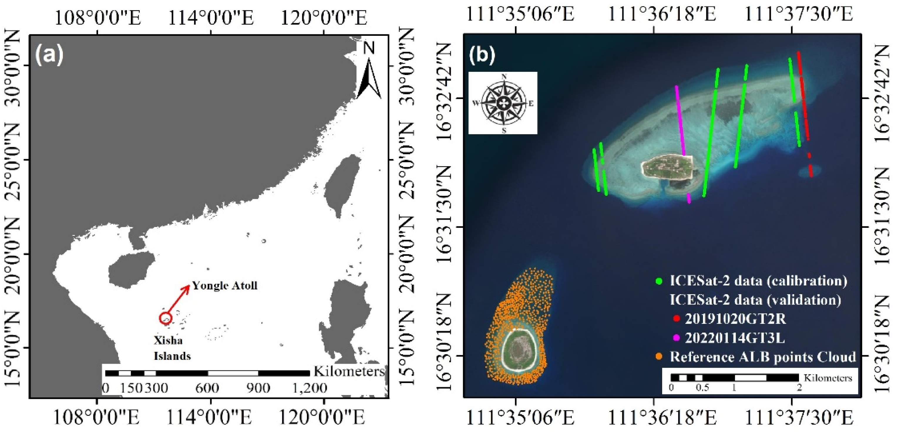
2.1. Study Area

As shown in Figure 1a, our study area was located in the Yongle Atoll, which is a part of the Xisha Islands. The Xisha Islands are one of the four islands in the South China Sea, which consists of 22 islands, 7 sandbanks, and more than 10 sunken reefs. Our experimental data were distributed in Shanhu Island and Ganquan Island. The area of Shanhu Island including the main reef is approximately 5 km² with an east to west distance of approximately 3.5 km. The central location of Shanhu Island is 111°36′E, 16°32′N. Ganquan Island lies northwest of the Yongle Islands at 16°30′N, 111°35′E. The area of Ganquan Island including the main reef is approximately 1.2 km².

2.2. ICESat-2 ATL03 Dataset

ICESat-2 ATL03 Global Geolocated Photon Data were produced from ATL02 ATLAS L1B Converted Telemetry Data. There are six “gtx” groups, with each group containing segments for one laser beam of the ground track (three strong and three weak beams). Each “gtx” group contains the latitude, longitude, time, height above the WGS-84 ellipsoid, classified mark, and confidence for all the raw photons. During the preprocessing of the ATLAS data, a large number of ground tracks were excluded due to data discontinuity and failure to extract effective underwater photons. Therefore, in this study, seven ground tracks from six ATL03 datasets were finally selected and processed to acquire the bathymetric points (

Table 1. Acquisition time and geodetic coordinate distribution of the advanced topographic laser altimeter system datasets.

ATL03 Dataset	Time (Local)	Track Used	Geodetic Coordinate Distribution
20181022	15:38	GT1R	111.626°E, 16.532°N−111.624°E, 16.553°N
20190222	21:51	GT3L	111.618°E, 16.552°N−111.616°E, 16.533°N
20190421	06:58 *	GT1L	111.597°E, 16.530°N−111.596°E, 16.537°N
20190524	17:31	GT2L	111.614°E, 16.549°N−111.612°E, 16.529°N
20191020	22:17	GT1R	111.598°E, 16.529°N−111.597°E, 16.537°N
	22:17	GT2R (Validation)	111.628°E, 16.530°N−111.625°E, 16.552°N
20220114	07:20 *	GT3L (Validation)	111.608°E, 16.547°N−111.610°E, 16.526°N

* Represent that the date of the local time was the day after the date of the data acquisition.

). Furthermore, five of the seven ground tracks were used for in situ water depths to feed the SDB models. The remaining two ground tracks, 20191020GT2R and 20220114GT3L (red and pink solid lines, respectively, in Figure 1b), were used as reference water depths to evaluate the performance of the SDB models.

2.3. Spaceborne Images and Reference ALB Data

A spaceborne hyperspectral imagery, the standard Zhuhai-1 Orbita HyperSpectral (OHS) Level-1B product acquired on 13:06 of local time, 7 January 2020, was selected. Zhuhai-1 is a micro nano satellite constellation developed by Zhuhai Orbita Aerospace Technology Co., Ltd., Zhuhai, China. It was designed to be composed of 34 remote sensing micro-nano satellites. Currently, there are eight hyperspectral satellites in orbit, including OHS-2A/B/C/D and OHS-3A/B/C/D. The Zhuhai-1 hyperspectral satellite adopts the push-broom imaging method. The spatial resolution is 10 m, and the spectral resolution is 2.5 nm, with the wavelength between 400 and 1000 nm [43]. Due to the limitation of compression and storage, it is designed to downlink data of default 32 bands (

Table 2. Band information and spatial resolution for Zhuhai-1 and Sentinel-2A.

Zhuhai-1						Sentinel-2A
Band	Wavelength (nm)	Resolution (m)	Band	Wavelength (nm)	Resolution (m)	Band	Wavelength (nm)	Resolution (m)
1	440–446	10	17	708–710	10	1	433–453	60
2	462–469	10	18	729–731	10	2	458–523	10
3	486–494	10	19	745–747	10	3	543–578	10
4	496–504	10	20	759–761	10	4	650–680	10
5	505–514	10	21	775–777	10	5	698–713	20
6	526–535	10	22	779–781	10	6	733–748	20
7	545–555	10	23	805–807	10	7	773–793	20
8	554–565	10	24	819–821	10	8	785–900	10
9	574–585	10	25	832–834	10	9	935–955	60
10	590–602	10	26	849–851	10	10	1360–1390	60
11	619–621	10	27	863–866	10	11	1565–1655	20
12	639–641	10	28	878–881	10	12	2100–2280	20
13	664–666	10	29	894–897	10
14	669–671	10	30	908–912	10
15	685–687	10	31	923–930	10
16	699–701	10	32	937–944	10

). The spectrum bands could be re-selected by uploading commands. Multiple CMOS detectors with gradient spectral filter were employed to receive the energy of different bands. The uncontrolled positioning accuracy of Zhuhai-1 is greater than 500 m, and the controlled positioning accuracy is less than 3 pixels. The Zhuhai-1 data were stored with quantitative range of 10 bits. The relative radiometric calibration error is less than 3%, and the signal-to-noise ratio is 25–40 dB (solar altitude > 30° and surface reflectance > 0.2). The image used in this study was obtained from OHS-3D with cloud cover less than 10%.

In addition, for the comparison of SDB results between hyperspectral and convenient multispectral images, a standard Sentinel-2A Multispectral Instrument Level-2A product acquired on 10:56 of local time, 5 March 2021, was downloaded on from the Copernicus data center (https://scihub.copernicus.eu/dhus/#/home, 13 October 2021) of the European Space Agency. Four bands with spatial resolution of 10 m, including bands 2, 3, 4, and 8, were used for subsequent analysis.

The reference ALB data for Ganquan Island (orange solid circles in Figure 1b) were acquired on 15:38 of local time, 9 January 2013, using a scanned hydrographic operational airborne LiDAR system (SHOALS-3000, Vaughan, ON, Canada). Using a green laser light (532 nm) at 3000 pulses per second, this ALB system has a nominal bathymetric accuracy of 0.3 m [44,45].

2.4. Satellite-Derived Bathymetry Models

Based on spaceborne images and ATL03 bathymetric points, two traditional empirical models were trained to generate bathymetric maps. The linear band model developed by Lyzenga et al. uses log-transformed linear reflectance as the independent variable to estimate water depths (Equation (1)):

$$h_w=a_0+{\displaystyle \sum _{i=1}^k{a}_i\ln [R_w({\lambda }_i)]}$$

(1)

The second model is the widely used band ratio model proposed by Stumpf et al. (Equation (2)), which uses a ratio logarithmic transformation to capture the relationship between reflectance and in situ water depth:

$$h_w=m_0\times \frac{\ln \left[c\times R_w({\lambda }_i)\right]}{\ln \left[c\times R_w({\lambda }_j)\right]}+m_1$$

(2)

In the above two models, $h_w$ is the water depth derived from the spaceborne image, and $R_w({\lambda }_i)$ and $R_w({\lambda }_j)$ are the above-water surface reflectance for bands i and j, respectively. c in Equation (2) is a fixed coefficient (generally set to 1000) to ensure that the logarithm is positive under any condition and that the ratio will produce a linear response with depth [21]. $a_0$, $a_i$, $m_0$, and $m_1$ were obtained by minimizing the difference between the estimated water depth and the in situ water depth.

2.5. Data Pre-Processing

All the ATL03 ground tracks were first processed using a filtering and refraction-correction algorithm [28,46]. In this algorithm, a density-based variable elliptical filter was employed to separate sea surface and seafloor photons from noisy raw ATL03 photons. The filtering algorithm includes the following steps: (1) the original photons were divided into segments along the height direction, and a Gaussian curve fitting was employed to capture the relationship between the center elevation and the photon numbers of the segments; (2) the above-water, water surface, and water column photons were separated by the parameters of the fitted Gaussian curve; (3) initial parameters of the elliptical filter were determined, and the water surface photons were detected; (4) the relationship between the initial ellipse filter and the water-column photon density was established; and (5) the bottom photons were detected by the variable elliptical filter.

To simplify the water refraction and facilitate the correction calculations, the instantaneous sea-surface was considered as a plane. Based on the instantaneous sea surface and the spatial relationship between the laser beams and the instantaneous sea surface, the refraction correction was applied. The refraction correction methods includes the following steps: (1) for each seafloor photon, the instantaneous sea-surface was reconstructed by the detected surface photons, which belongs to the same laser beam as the seafloor photon; (2) the displacements in the along-track, cross-track, and elevation directions were acquired based on the relationship of the laser beam, the incident angle, the refracted angle, and the transmission distance in the water column; (3) the final displacement in the elevation direction was obtained by the average of the corresponding elevation displacements in the along- and cross-track directions. Finally, the water depths were obtained by calculating the differences in elevations between the corrected seafloor photons and sea surface photons.

The Zhuhai-1 image was geometrically projected and atmospherically corrected based on ENVI 5.3 following the operating manual [43]. The atmospheric correction was processed with the fast line-of-sight atmospheric analysis of spectral hypercubes (FLAASH) process tool embedded in ENVI. FLAASH was derived from the radiative transfer model MODTRAN4 [47]. A series of parameters were needed to run the FLAASH, including but not limited to scene center location, sensor altitude, average ground elevation, pixel size, flight date, atmospheric model, and aerosol model. Some of these parameters were directly acquired from the raw Zhuhai-1 image, and the others were acquired from the other dataset (e.g., average ground elevation) or previous research (e.g., atmospheric model). The preprocessing of Sentinel-2 image was conducted automatically by the Sen2Cor, which is the ESA official procedure [48]. The atmospheric correction algorithm was based on the libRadtran radiative transfer model, generating a large look-up table of sensor-specific functions (path radiance, direct and diffuse transmittances, direct and diffuse solar fluxes, and spherical albedo) that account for a wide variety of atmospheric conditions, solar geometries, and ground elevations [49].

Tide correction was required to calibrate and validate the SDB models. In this study, tide correction was conducted based on the tide model NAO.99b [50], a global ocean tide model representing 16 major constituents with a spatial resolution of 0.5°. The constituents were estimated by assimilating approximately five years of TOPEX/Poseidon altimeter data into a barotropic hydrodynamic model [51]. The tidal height of the ATL03 ground tracks, the images, and the in situ ALB data were acquired by inputting the location and the precise acquisition time into the tidal model.

2.6. Evaluation of the Performances of the SDB Models

To estimate the accuracy of the SDB results based on Zhuhai-1 hyperspectral imagery and ICESat-2 bathymetric points, the estimated water depths were compared with the bathymetric results of two ATL03 ground tracks and ALB water depths at Ganquan Island, respectively. The coefficient of determination (R²), bias, and root mean square error (RMSE) were calculated and used to evaluate the performance of the SDB models.

3. Results

To ensure the bathymetric reliability of the ATL03 data, the filtering and bathymetric results were illustrated in Section 3.1. Furthermore, the correlation between the products generated by the reflectance of two or three bands (Zhuhai-1 and Sentinel-2) and the “in situ” water depth acquired from the five ATL03 ground tracks were analyzed. Based on the results of the correlation analysis, ten SDB models were calibrated, and the bathymetric maps were generated. The accuracy of the calibration and the bathymetric maps are shown in Section 3.2 and Section 3.3, respectively. Moreover, to investigate the performances of the SDB models, the bathymetric maps were validated by two ATL03 ground tracks, 20191020GT2R and 20220114GT3L, and the results are illustrated in Section 3.4.1. Lastly, to clarify the robustness of the SDB models, the bathymetric maps were validated using the ALB results at Ganquan Island, and the results are illustrated in Section 3.4.2.

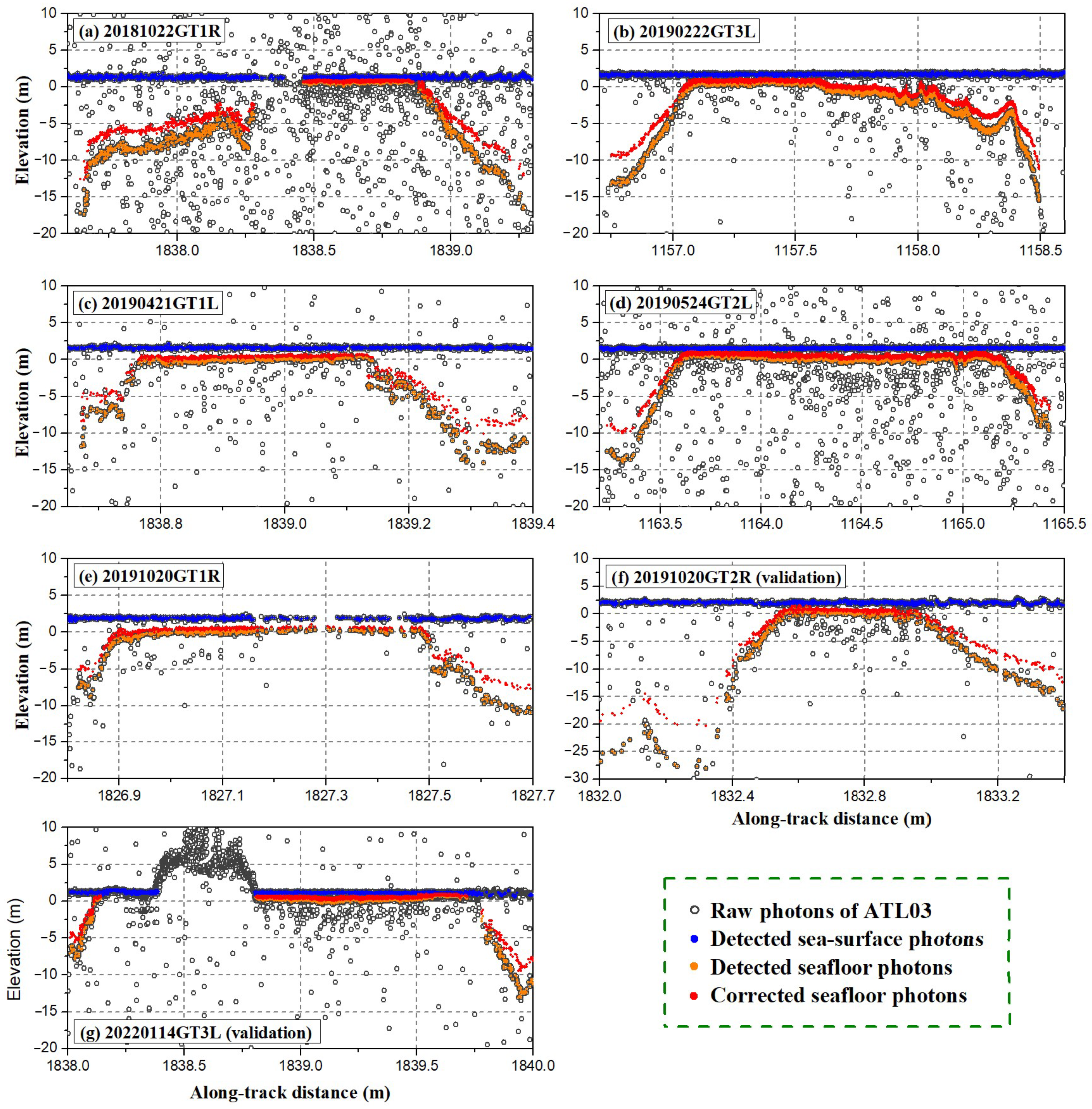
3.1. Signal Photon Detection and Bathymetry of ATL03

Due to the large coral reef flat of Shanhu Island, extremely shallow-water areas were observed in every ground track, for example, the signal photons with the along-track distance between 1838.5 and 1838.8 km. Due to the attenuation of water on laser energy, the number of the seafloor photons decreased rapidly with the increase in water depth at the edge of the coral reef flat. Although different densities and spatial distributions of the raw photons were observed for the six ATL03 ground tracks, the sea surface and seafloor photons were successfully detected (Figure 2a–f). As shown in

Table 3. Number of detected signal photons and maximum bathymetric results after refraction correction for seven ATL03 ground tracks used at Shanhu Islands.

Ground Track	Number of Detected Sea-Surface Photons	Number of Detected Bottom Photons	Maximum Water Depth after Correction (m)
20181022GT1R	2891	2027	13.61
20190222GT3L	4922	3658	14.89
20190421GT1L	1166	881	11.70
20190524GT2L	4170	2514	12.01
20191020GT1R	941	568	9.64
20191020GT2R	880	795	23.58
20220114GT3L	5336	3534	10.61

, due to the different lighting environment during the data acquisition, as well as the filtering algorithm, the number of the detected signal photons was different for the ATL03 ground tracks. Ground track 20190222GT3L was acquired at the local time of 21:51 (UTC+8:00), while 20191020GT1R and 20191020GT2R were acquire at the local time of 22:17 (UTC+8:00); therefore, these ground tracks had fewer noisy photons than the other tracks. The maximum water depth of 23.58 m was acquired by the ground track 20191020GT2R, while the maximum water depths of the other ground tracks were close, ranging from 9.64 to 14.89 m.

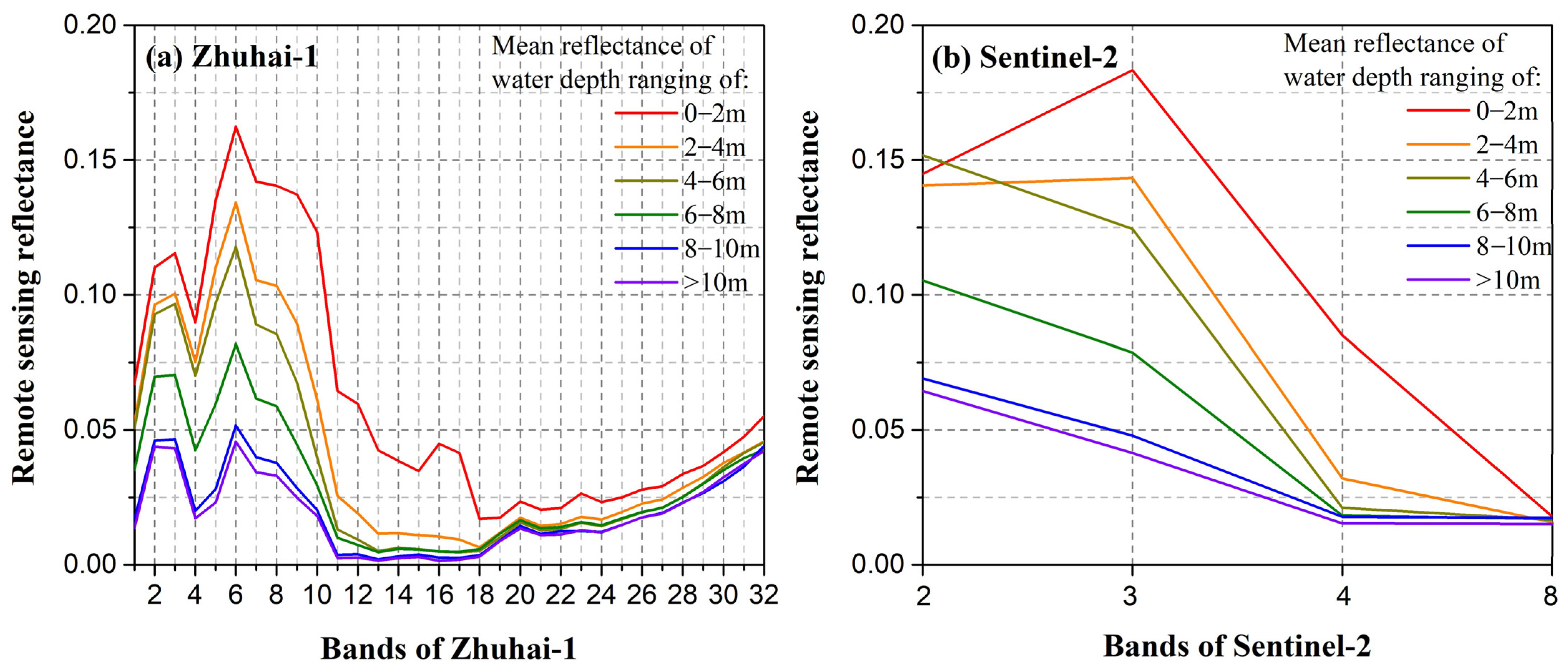
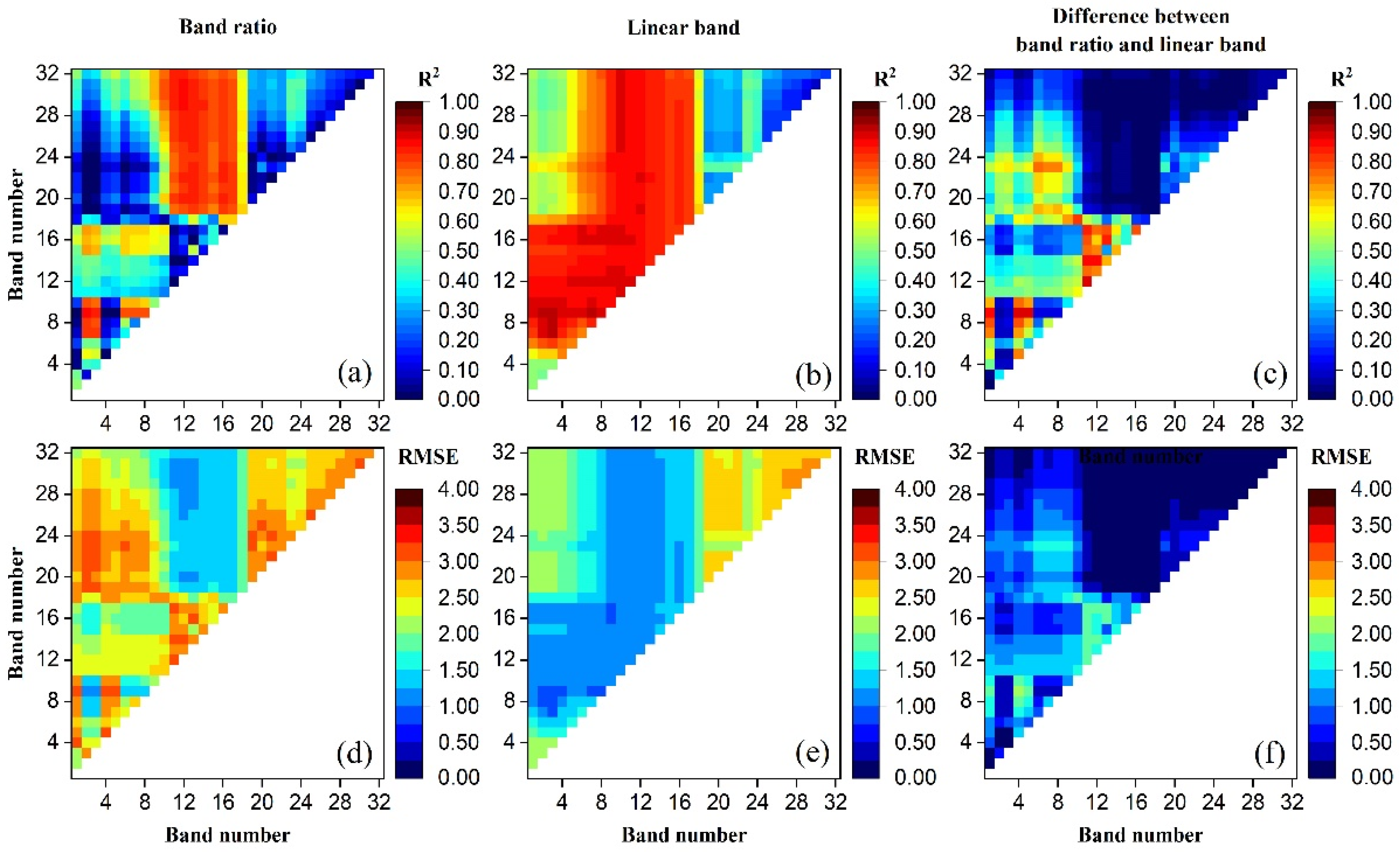
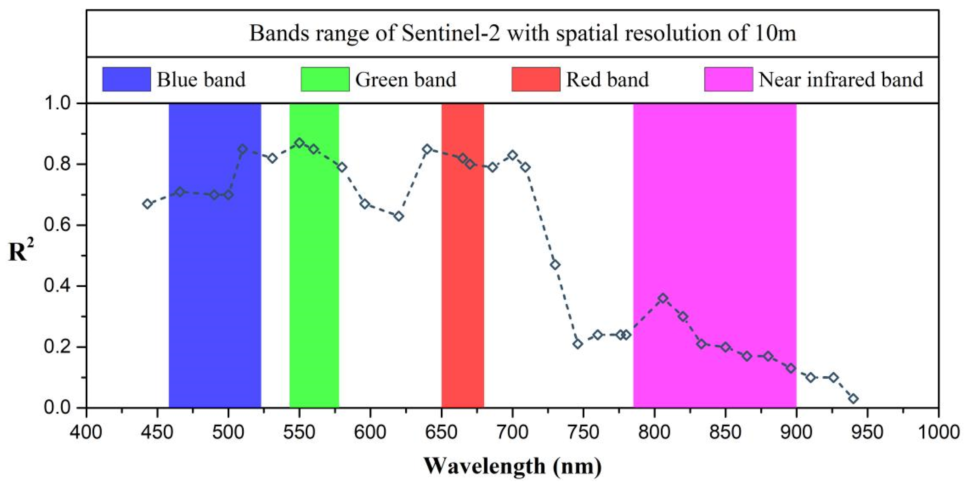
3.2. Band Selection for Zhuhai-1 Bathymetry

Compared with Sentinel-2, Zhuhai-1 has more band choices for shallow-water bathymetry. The mean values of the remote sensing reflectance for Zhuhai-1 and Sentinel-2 at different intervals of the ICESat-2 water depths are illustrated in Figure 3. As shown in Figure 3, the characteristics of the reflectivity change varied for different bands. In the near-infrared bands (band 8 for Sentinel-2 and bands 18–32 for Zhuhai-1), the decrease in water depth had almost no effect on the reflectance. In the red bands (band 4 for Sentinel-2 and bands 12–17 for Zhuhai-1), the reflectance clearly decreased at water depths in the intervals of 0–2 m to 2–4 m. However, the reflectance became insensitive as the water depth continued to increase. In addition, in the remaining blue and green bands, the reflectance of the bands decreased with increasing water depth.

Before the SDB models were calibrated, the tidal correction was applied. Tidal heights of the ATL03 ground tracks, images, and in situ ALB data are shown in

Table 4. Tidal height produced by NAO.99b for the ATL03 ground tracks, remote sensing images, and the in situ ALB data.

Calibration Data	Tidal Height (m)	Images	Tidal Height (m)	Validation Data	Tidal Height (m)
20181022GT1R	−0.3020	Zhuhai-1	0.2515	20191020GT2R	0.3392
20190222GT3L	0.1755	Sentinel-2	−0.1634	20220114GT3L	−0.4327
20190421GT1L	0.0372			ALB data	0.8168
20190524GT2L	0.1135
20191020GT1R	0.3392

. For the five ground tracks used for calibration, the tidal heights ranged from −0.3020 to 0.3392 m. The maximum tidal difference between the five ground tracks and the Zhuhai-1 image was 0.5535 m, and the corresponding value was 0.5026 m for Sentinel-2 image.

To investigate the suitable bands of Zhuhai-1 for bathymetry, we randomly selected two bands following the forms of band ratio and linear band models to calibrate the SDB models. As shown in Figure 4a,b, the high correlation (R² > 0.8) of the SDB models is mainly distributed in two areas of band selection. A suitable dual-band selection strategy is to choose two bands from blue to green light (bands 1 to 9 of Zhuhai-1), while another strategy is to choose one band from the red bands (bands 10–17 of Zhuhai-1) and the other from the near-infrared bands (bands 19–32). When two suitable bands were selected by the two strategies, the R² between the depths of the ground tracks and the estimated depths were over 0.8; additionally, RMSEs were less than 1.5 m.

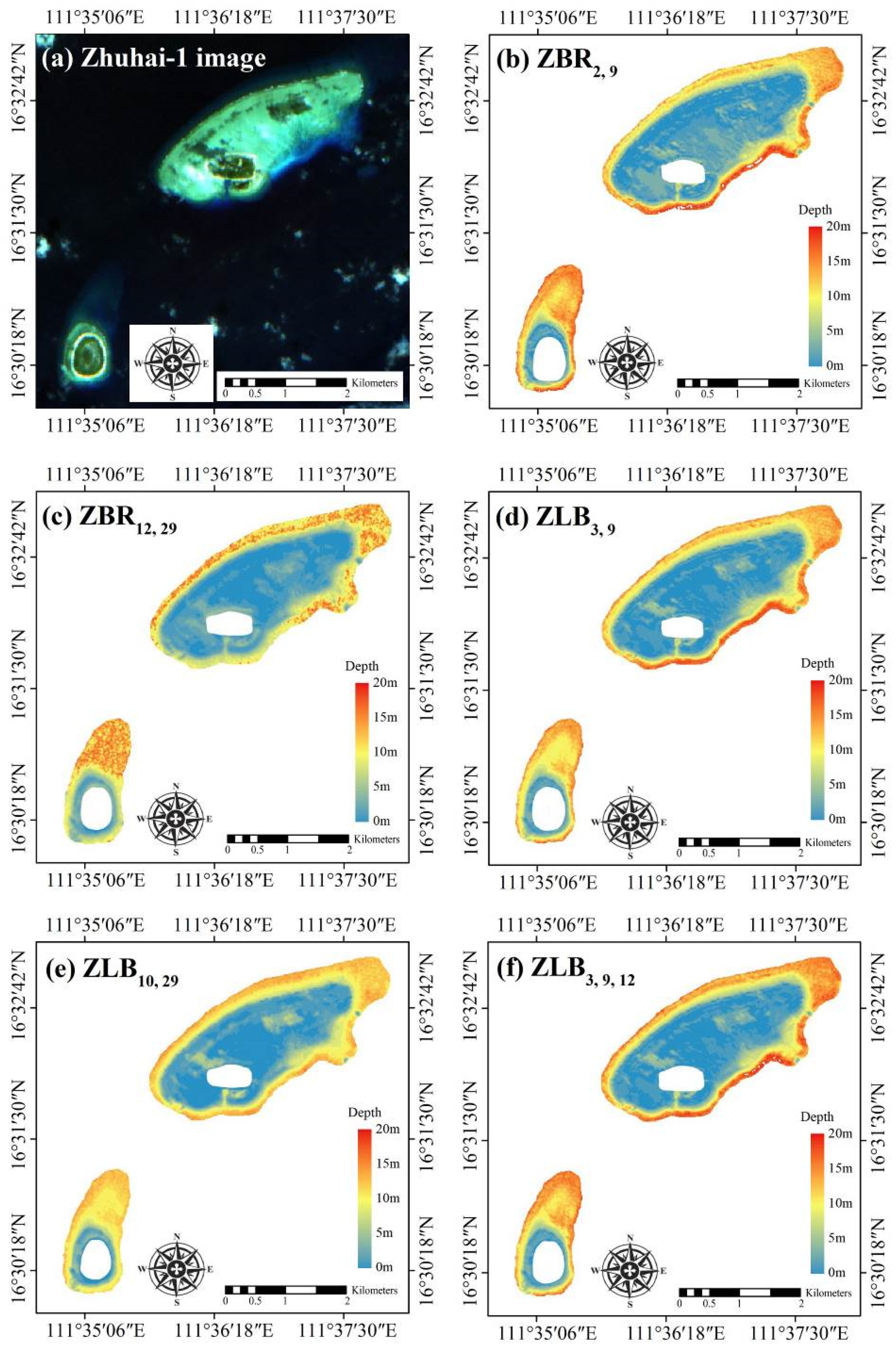
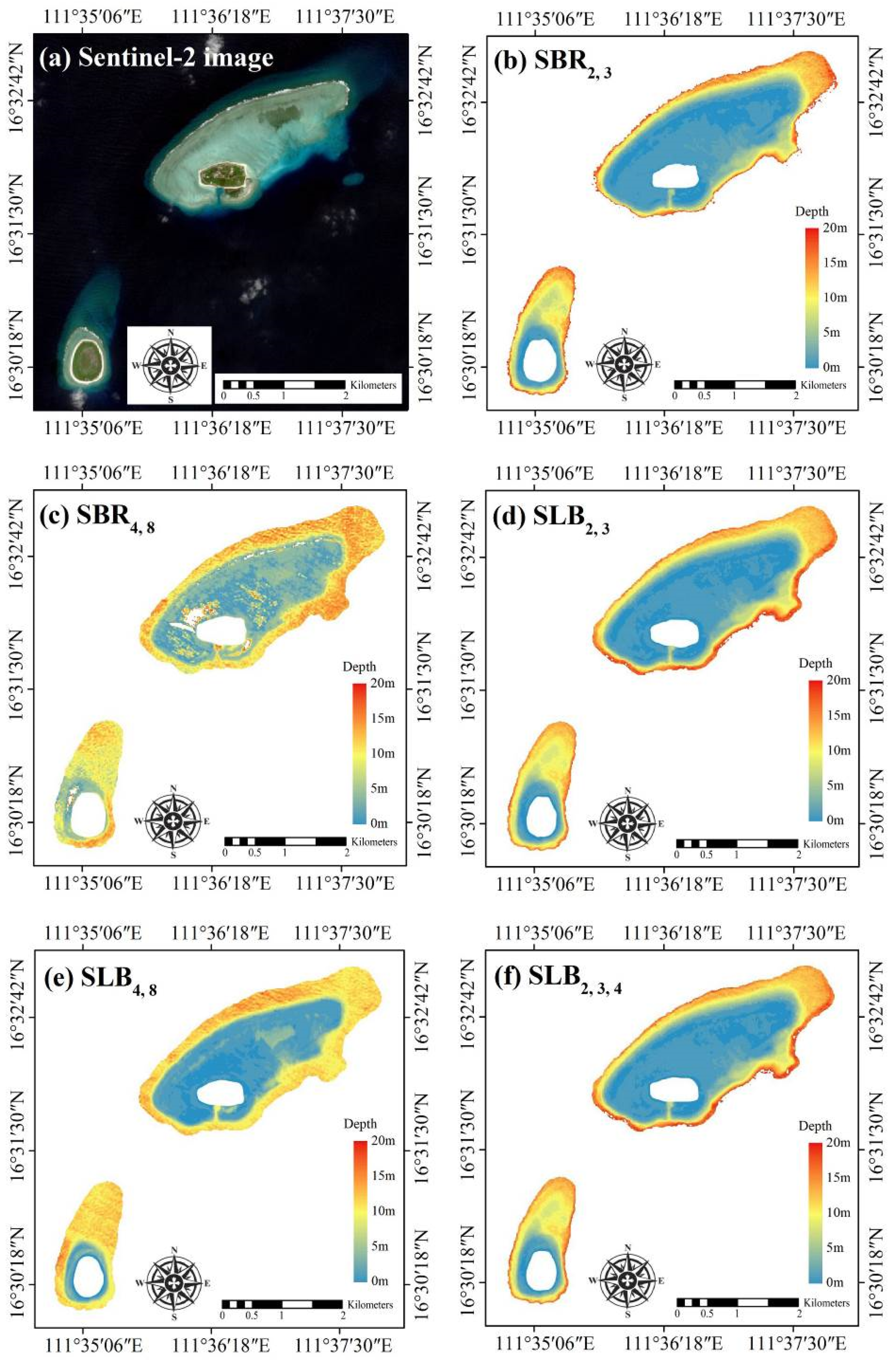
3.3. Calibration of the SDB Models and Bathymetric Mapping

Based on the preliminary statistical test described in the previous section, five models —two band ratio models and three linear band models—were employed to generate the bathymetric mapping for the Zhuhai-1 and Sentinel-2 images (

Table 5. Band selection, forms, parameters, and accuracy (represented by R² and RMSE) of the calibrated satellite-derived bathymetry models in this research. Abbreviations: B, blue light; G, green light; R, red light, NI, near-infrared light; ZBR, Zhuhai-1 band ratio; ZLB, Zhuhai-1 linear band; SBR, Sentinel-2 band ratio; SLB, Sentinel-2 linear band; RMSE, root mean square error.

Satellite	Bands	Models	Abbreviation of Models	R2	RMSE (m)	Equation
Zhuhai-1	2 (B) 9 (G)	Band ratio	ZBR2, 9	0.90	0.94	$h_w=34.0142\times \frac{\ln \left[1000\times R_w(B2)\right]}{\ln \left[1000\times R_w(B9)\right]}-31.2315$
	12 (R) 29 (NI)	Band ratio	ZBR12, 29	0.93	0.81	$h_w=-10.2619\times \frac{\ln \left[1000\times R_w(B12)\right]}{\ln \left[1000\times R_w(B29)\right]}+12.1409$
	3 (B) 9 (G)	Linear band	ZLB3, 9	0.92	0.86	$h_w=21.7878+4.4890\times \ln \left[R_w(B3)\right]-7.2544\times \ln \left[R_w(B9)\right]$
	10 (R) 29 (NI)	Linear band	ZLB10, 29	0.88	1.07	$h_w=25.6922-3.9649\times \ln \left[R_w(B10)\right]+0.6023\times \ln \left[R_w(B29)\right]$
	3 (B) 9 (G) 12 (R)	Linear band	ZLB3, 9, 12	0.92	0.85	$\begin{array}{l}{h}_w=20.9437+4.0060\times \ln \left[R_w(B3)\right]-\\ 6.3869\times \ln \left[R_w(B9)\right]-0.3196\times \ln \left[R_w(B12)\right]\end{array}$
Sentinel-2	2 (B) 3 (G)	Band ratio	SBR2, 3	0.91	0.89	$h_w=50.2883\times \frac{\ln \left[1000\times R_w(B2)\right]}{\ln \left[1000\times R_w(B3)\right]}-46.6726$
	4 (R) 8 (NI)	Band ratio	SBR4, 8	0.73	1.53	$h_w=-9.6127\times \frac{\ln \left[1000\times R_w(B4)\right]}{\ln \left[1000\times R_w(B8)\right]}+16.2537$
	2 (B) 3 (G)	Linear band	SLB2, 3	0.96	0.57	$h_w=18.6427+8.2569\times \ln \left[R_w(B2)\right]-10.3346\times \ln \left[R_w(B3)\right]$
	4 (R) 8 (NI)	Linear band	SLB4, 8	0.81	1.31	$h_w=20.5107-3.7745\times \ln \left[R_w(B4)\right]+1.1431\times \ln \left[R_w(B8)\right]$
	2 (B) 3 (G) 4 (R)	Linear band	SLB2, 3, 4	0.96	0.56	$\begin{array}{l}{h}_w=18.1009+8.7426\times \ln \left[R_w(B2)\right]-\\ 10.9857\times \ln \left[R_w(B3)\right]+0.2867\times \ln \left[R_w(B4)\right]\end{array}$

). For convenience, the names of the models were simplified based on the source imagery, model form, and selected bands. For instance, the band ratio model using bands 2 and 9 of Zhuhai-1 was named ZBR_{2, 9}. As shown in Table 5, for the Zhuhai-1 image, high correlations were observed for all the calibration models (R²: 0.88–0.96, RMSE: 0.57–1.07 m). ZBR_{12, 29} was the optimal model, with an R² of 0.93 and RMSE of 0.81 m. For the Sentinel-2 image, calibration models including blue and green bands (SBR_{2, 3}, SLB_{2, 3}, and SLB_{2, 3, 4}) showed high accuracy with R² > 0.9 and RMSE < 1 m. However, calibration models using red and near-infrared bands (SBR_{4, 8} and SLB_{4, 8}) showed slightly poor accuracy with an R² of 0.73 and 0.81 and RMSE of 1.53 and 1.31 m, respectively. In addition, compared with that of linear dual-band models using blue and green bands (ZLB_{3, 9} and SLB_{2, 3}), the accuracy of the linear three-band model, which introduced information from the red band (ZLB_{3, 9, 12} and SLB_{2, 3, 4}), was not significantly improved for either Zhuhai-1 or Sentinel-2 imagery.

The bathymetric maps produced from the Zhuhai-1 and Sentinel-2 images based on the SDB models are shown in Figure 5 and Figure 6, respectively. Although the spatial distributions of the water depths were visually similar for both images and all models, some obvious differences were observed. For Zhuhai-1 image, bathymetric maps of models ZBR_{2, 9}, ZLB_{3, 9}, and ZLB_{3, 9, 12} showed better performance than models ZBR_{12, 29} and ZLB_{10, 29}. The SDB results of ZBR_{12, 29} (Figure 5c) were unable to exhibit the variation in water depth north of Ganquan Island and at the periphery of Shanhu Island where the water was deeper than 12 m. The SDB results of ZBR_{10, 29} (Figure 5e) were able to show the variation in water depth in these two areas; however, the bathymetric results were slightly underestimated compared to those of the other models. For Sentinel-2, models SBR_{4, 8} and SLB_{4, 8} in Figure 6c,e showed poor performance. Moreover, it is worth noting that the bathymetric results for all models and both images were highly consistent with each other in extremely shallow areas with depths < 5 m.

3.4. Validation and Error Analysis of the SDB Models

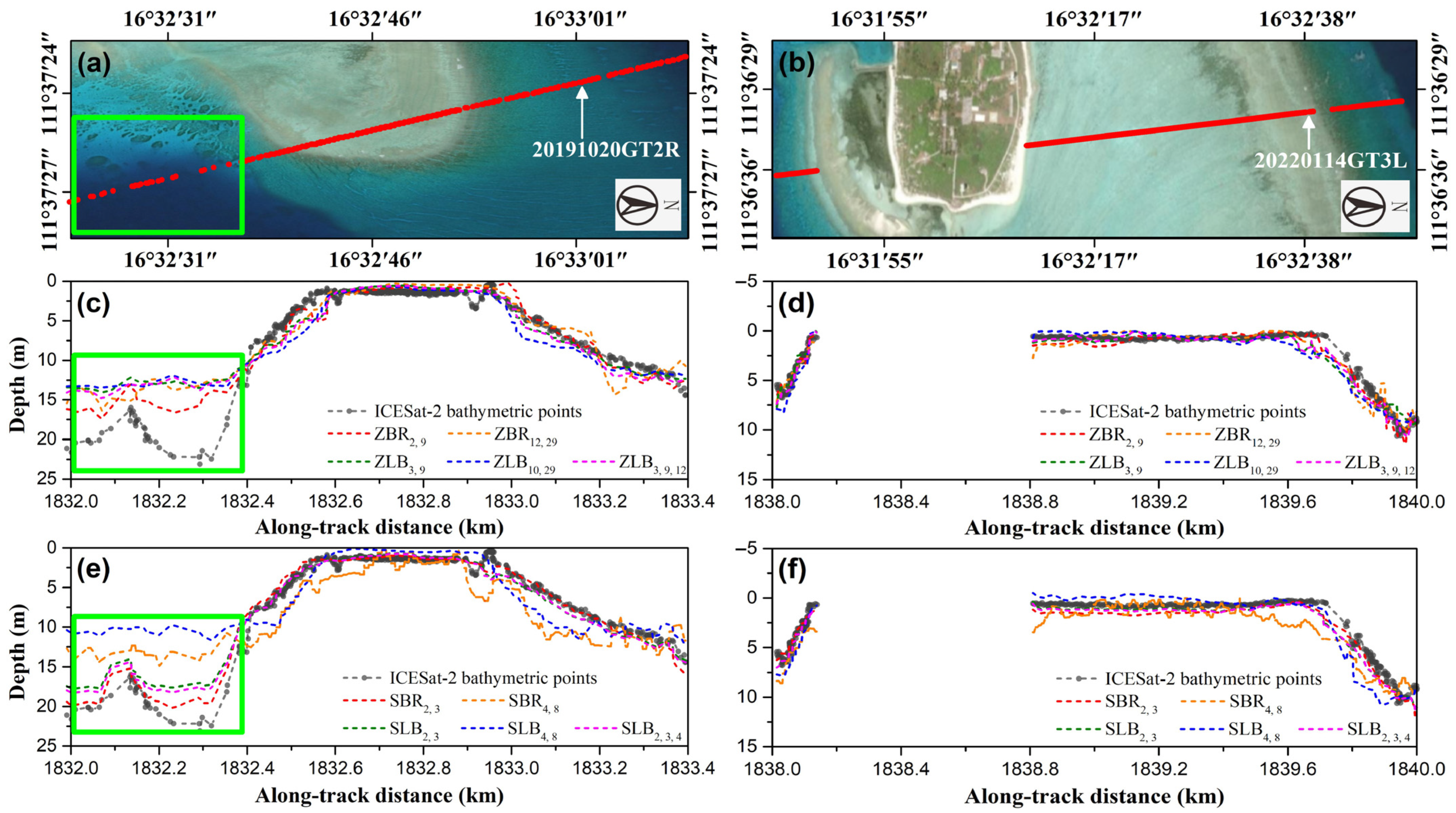
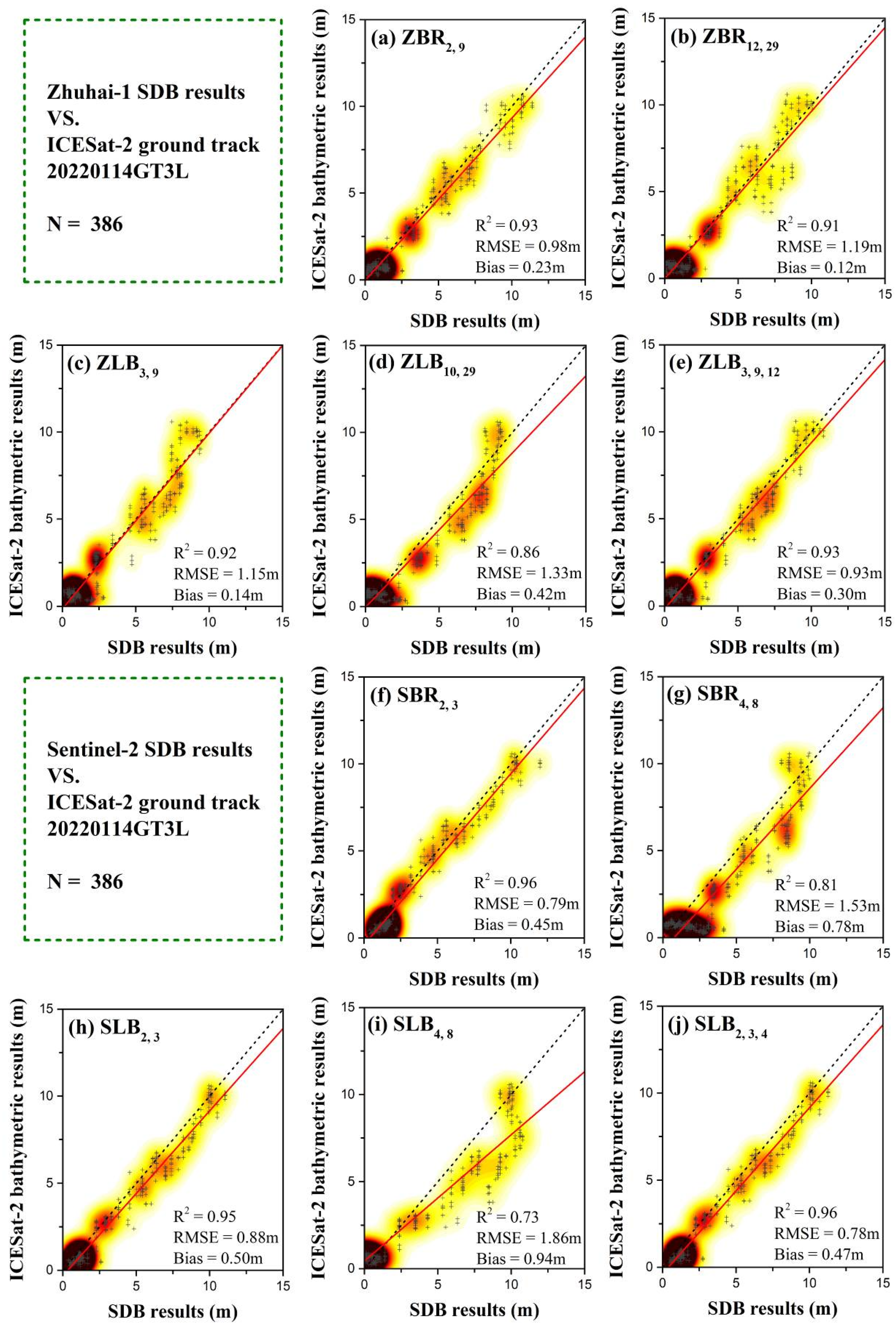
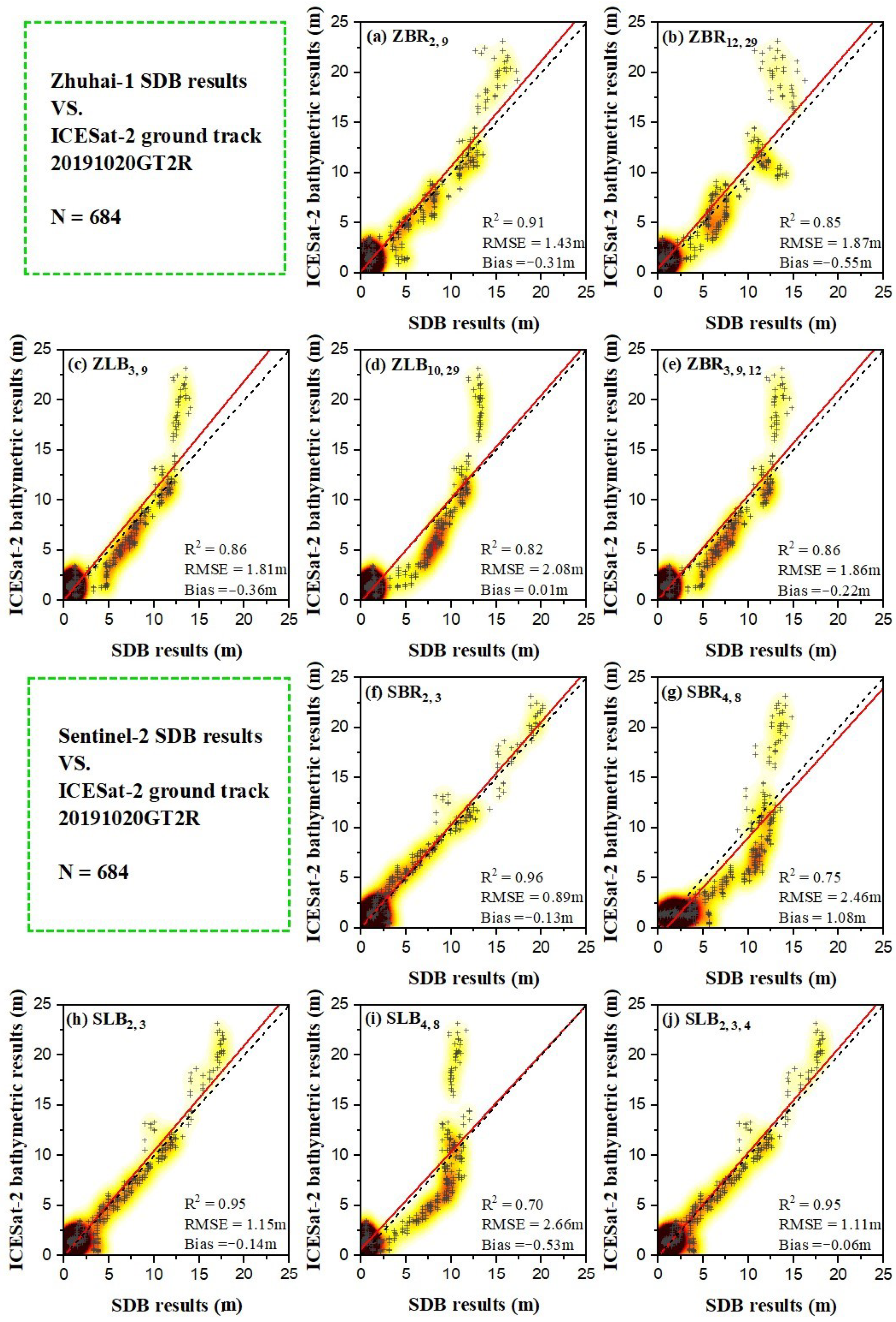
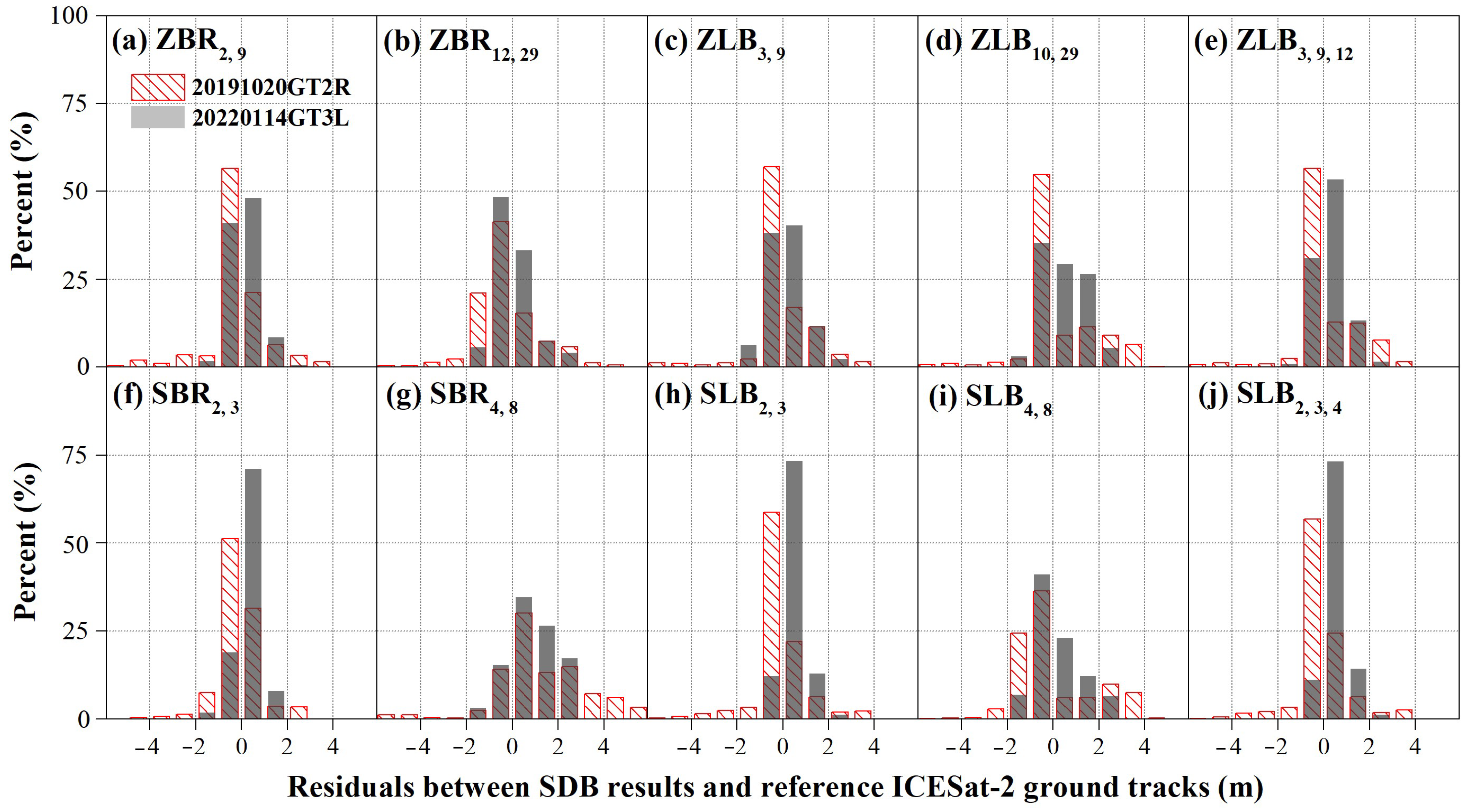
3.4.1. Validation Using ATL03 Ground Tracks

To investigate the bathymetric capability and accuracy of Zhuhai-1, the SDB results were first compared with the bathymetric profile of the ICESat-2 ground track 20191020GT2R and 20220114GT3L (Figure 7). Ground track 20191020GT2R overlapped with the northeast of Shanhu Island. From south to north, the footprint of the laser beams first covered a segment with water depth ranging from deep to shallow, then moved away from the reef flat of shallow water, and finally returned to a segment with increasing depth. The bathymetric profile of 20191020GT2R was in accordance with the underwater topography with the along-track distance between 1832.4 and 1833.4 km. However, as the green rectangle illustrated in Figure 7a,c,e, all the SDB profiles were significantly shallower than the ICESat-2 profiles when the depth was greater than 12 m. As shown in Figure 8, when using the 20191020GT2R (684 bathymetric points) as validation data, ZBR₂, ₉ showed the best performance for Zhuhai-1 image with R² of 0.91, RMSE of 1.43, and bias of −0.31 m, and SBR_{2, 3} showed the best performance for Sentinel-2 image with R² of 0.96, RMSE of 0.89, and bias of −0.13 m. As shown in Figure 9, most of the residuals were distributed between −2 m and 2 m for all the SDB models. However,

Table 6. Distribution of RMSE and bias between ground track 20191020GT2R and 20220114GT3L and satellite-derived bathymetry (SDB) results with different intervals of water depth.

Ground Tracks for Validation	SDB Models	Parameters (m)	Intervals of Water Depth (m)
			[0, 2]	[2, 4]	[4, 6]	[6, 8]	[8, 10]	[10, 12]	[12, 14]	[>14]
20191020GT2R	ZBR2, 9	RMSE	0.81	1.57	1.22	0.95	1.18	1.24	1.02	4.69
		bias	−0.21	−0.74	0.61	0.50	0.40	1.06	−0.53	−4.33
	ZBR12, 29	RMSE	0.88	1.89	1.56	1.04	1.70	1.40	2.03	6.32
		bias	−0.59	0.21	1.29	−0.27	1.01	0.88	−1.80	−5.69
	ZLB3, 9	RMSE	0.85	1.56	1.58	0.92	0.83	0.66	1.74	6.6
		bias	−0.33	0.44	1.52	0.82	0.67	0.45	−1.46	−6.32
	ZLB10, 29	RMSE	0.75	2.53	2.86	1.76	1.38	0.69	1.65	6.51
		bias	−0.18	1.43	2.84	1.69	1.35	0.48	−1.47	−6.15
	ZLB3, 9, 12	RMSE	0.84	1.72	1.87	1.15	1.47	1.22	1.32	6.28
		bias	−0.32	0.54	1.78	1.03	1.20	1.10	−0.94	−5.93
	SBR2, 3	RMSE	0.68	0.83	0.97	0.71	0.54	1.17	2.81	3.6
		bias	0.09	−0.62	−0.75	−0.35	0.16	0.54	−1.41	−3.11
	SBR4, 8	RMSE	1.61	2.27	3.42	3.32	2.41	1.32	1.73	6.35
		bias	0.84	2.09	3.23	3.25	2.20	0.86	−1.04	−6.10
	SLB2, 3	RMSE	0.91	0.88	0.71	0.81	0.87	0.96	2.3	4.08
		bias	−0.07	−0.01	0.21	0.55	0.79	0.54	−1.53	−4.79
	SLB4, 8	RMSE	1.03	2.37	3.15	2.9	1.26	1.08	2.95	7.45
		bias	−0.73	0.89	3.11	2.83	1.10	−0.81	−2.80	−7.37
	SLB2, 3, 4	RMSE	0.93	0.79	0.71	0.78	0.94	1.08	2.24	3.65
		bias	0.01	−0.03	0.07	0.49	0.86	0.72	−1.35	−3.32
20220114GT3L	ZBR2, 9	RMSE	0.71	0.86	1.05	1.16	1.21	1.05	-	-
		bias	0.14	0.32	0.41	0.20	0.67	0.04	-	-
	ZBR12, 29	RMSE	0.80	1.06	1.63	1.50	0.90	1.44	-	-
		bias	0.09	0.42	0.75	−0.13	−0.54	−1.01	-	-
	ZLB3, 9	RMSE	0.64	0.82	1.07	0.89	1.16	1.73	-	-
		bias	0.23	−0.13	0.68	0.30	−0.92	−1.59	-	-
	ZLB10, 29	RMSE	1.04	1.22	1.47	1.29	1.56	2.13	-	-
		bias	0.05	1.09	1.60	1.14	−0.37	−1.33	-	-
	ZLB3, 9, 12	RMSE	0.80	0.85	1.31	0.95	0.60	1.07	-	-
		bias	0.20	0.32	0.93	0.46	0.08	−0.48	-	-
	SBR2, 3	RMSE	0.91	0.69	0.87	1.13	1.18	1.22	-	-
		bias	0.66	−0.19	0.07	0.38	0.81	0.54	-	-
	SBR4, 8	RMSE	1.62	1.56	2.15	1.82	1.02	1.69	-	-
		bias	0.95	1.16	1.65	1.48	0.10	−1.36	-	-
	SLB2, 3	RMSE	0.72	0.88	1.22	1.26	0.99	0.76	-	-
		bias	0.43	0.31	0.81	0.84	0.66	0.09	-	-
	SLB4, 8	RMSE	0.89	1.9	2.4	2.53	1.29	0.74	-	-
		bias	−0.40	1.12	1.99	2.18	0.82	−0.44	-	-
	SLB2, 3, 4	RMSE	0.79	0.84	1.18	1.25	1.09	0.84	-	-
		bias	0.51	0.25	0.74	0.81	0.76	0.23	-	-

showed that all SDB results significantly underestimated water depth when the depth was greater than 12 m. The maximal bias was less than −6 m, while the RMSE was over 6 m between the SDB models and 20191020GT2R points.

Ground track 20220114GT3L passed through a piece of land (Zhaoshu Island); thus, a gap was observed on the profile with the along-track distance between 1838.1 and 1838.8 km. Validation results using 20220114GT3L (386 bathymetric points) were significantly better than those of 20191020GT2R, with ZLB_{3, 9, 12} and SLB_{2, 3, 4} showing the best performance for Zhuhai-1 and Sentinel-2 image, respectively (Figure 10). Moreover, the bias remained between −2 and 2 m, and the RMSE was lower than 2 m in most cases (Table 6).

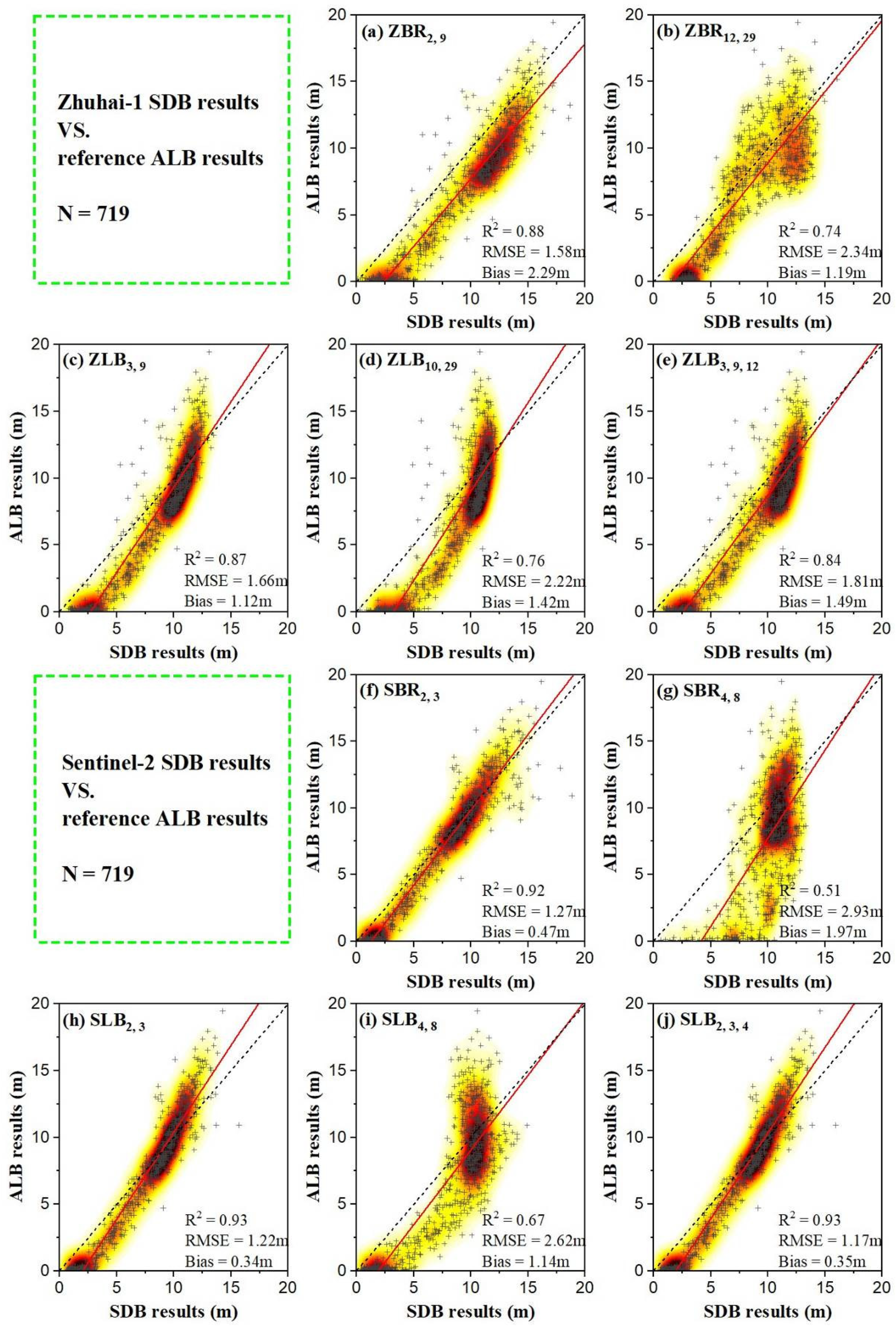
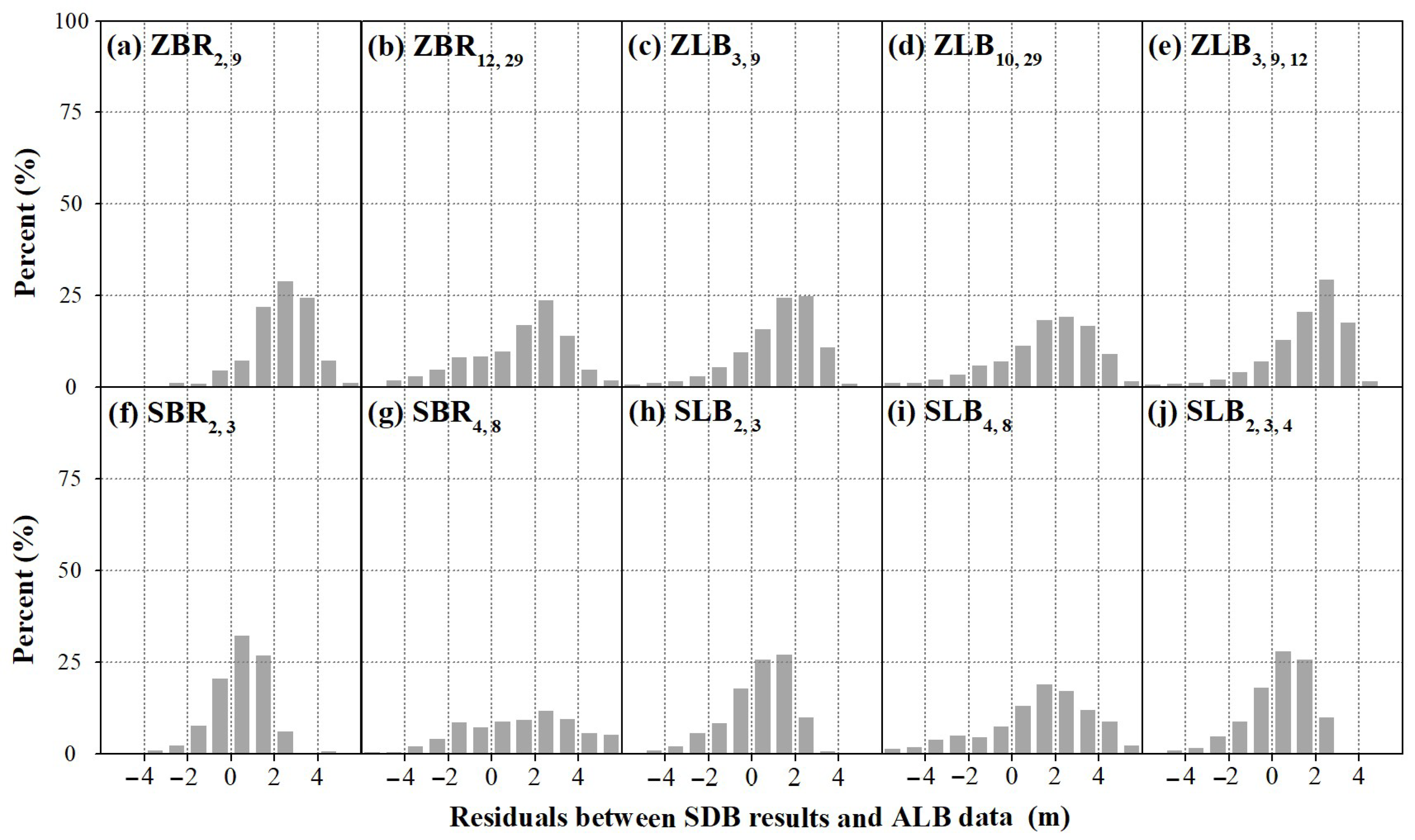
3.4.2. Validation Using ALB Data

To verify the robustness of the SDB models, the SDB results were also compared with the in situ ALB results at Ganquan Island (Figure 11). A total of 719 bathymetric points of ALB data were evenly distributed in the reef flat of the Ganquan Island. The correlation between the SDB models and the ALB results seemed to be smaller than that between SDB results and validation ATL03 ground tracks (R²: 0.51–0.93, RMSE: 1.17–2.93 m). SDB results slightly overestimated the depth when it was between 0 and 12 m (

Table 7. Distribution of RMSE and bias between ALB data and satellite-derived bathymetry (SDB) results with different intervals of water depth.

SDB Models	Parameters (m)	Intervals of Water Depth (m)
		[0, 2]	[2, 4]	[4, 6]	[6, 8]	[8, 10]	[10, 12]	[12, 14]	[>14]
ZBR2, 9	RMSE	2.34	2.70	2.51	2.65	2.50	1.98	1.50	1.14
	bias	2.25	2.62	2.43	2.61	2.48	1.71	0.64	−0.87
ZBR12, 29	RMSE	2.56	2.41	2.08	3.00	2.64	1.79	2.25	3.77
	bias	2.49	2.32	1.84	2.03	1.65	0.13	−1.62	−3.51
ZLB3, 9	RMSE	2.54	2.89	2.49	1.96	1.43	0.95	1.68	3.68
	bias	2.39	2.78	2.28	1.78	1.21	0.08	−1.49	−3.64
ZLB10, 29	RMSE	3.29	3.90	3.46	2.51	1.72	0.99	2.07	4.79
	bias	3.08	3.79	3.32	2.35	1.47	−0.02	−1.96	−4.72
ZLB3, 9, 12	RMSE	2.54	3.01	2.78	2.60	2.08	1.27	1.49	3.50
	bias	2.39	2.90	2.57	2.34	1.81	0.63	−1.03	−3.34
SBR2, 3	RMSE	1.39	1.43	1.15	0.81	0.95	1.46	1.70	2.22
	bias	1.29	1.33	0.85	0.49	0.38	0.04	−1.08	−2.14
SBR4, 8	RMSE	4.49	5.46	5.16	3.54	2.19	1.08	1.83	4.27
	bias	4.10	5.24	4.86	3.25	1.72	−0.19	−1.72	−4.10
SLB2, 3	RMSE	1.74	1.90	1.48	0.91	0.61	1.01	2.00	3.27
	bias	1.63	1.82	1.29	0.71	0.24	−0.59	−1.95	−3.35
SLB4, 8	RMSE	2.37	3.88	4.05	2.86	1.90	1.22	2.74	5.35
	bias	2.03	3.68	3.83	2.63	1.56	−0.29	−2.72	−5.34
SLB2, 3, 4	RMSE	1.72	1.79	1.38	0.86	0.62	1.01	1.90	3.07
	bias	1.61	1.71	1.17	0.66	0.24	−0.51	−1.82	−3.14

), while in most cases, more than 80% of the residuals were distributed between 0 and 4 m (Figure 12). However, this overestimation was not observed in comparisons of SDB results with ICESat-2 results for Shanhu Island.

4. Discussion

4.1. Comparison of Bathymetric Capability between Zhuhai-1 and Sentinel-2

The most commonly used band-combination strategy for shallow-water bathymetry may be the employment of blue and green bands, of which principle and potential have been revealed in previous research [52]. The blue and green bands of Sentinel-2 image have been widely and successfully used for shallow-water bathymetry [53]. In this study, relative high correlations were observed for the blue and green bands between Zhuhai-1 and Sentinel-2 (R² > 0.7, Figure 13). Moreover, the validation results of SDB models using blue and green bands of Zhuhai-1 (ZBR_{2, 9}, ZLB_{3, 9}, and ZLB_{3, 9, 12}) image showed a similar accuracy to that of Sentinel-2 image (SBR_{2, 3}, SLB_{2, 3}, and SLB_{2, 3, 4}), which further confirmed the potential of using the blue and green bands of Zhuhai-1 for shallow-water bathymetry.

Previous research demonstrated that the reflectance of the red band is sensitive in water, with depths < 5–6 m, which was available for bathymetry in extremely shallow areas [13,54]. Although the bathymetric accuracy did not improve significantly when the red band was added into the linear band model using blue and green bands, we could not completely ignore the effect of red bands for bathymetry in extremely shallow water of depths < 5 m. In this study, the red and near-infrared bands of Zhuhai-1, especially the red bands with short wavelength, contained more water-depth information than those of Sentinel-2. The SDB models using the red and near-infrared bands of Zhuhai-1 (ZBR_{12, 29} and ZLB_{10, 29}) image showed better performances than that of Sentinel-2 image (SBR_{4, 8} and ZLB_{4, 8}), which demonstrated the great potential of Zhuhai-1 for bathymetry in extremely shallow areas.

4.2. SDB Error Analysis

Previous studies have investigated the bathymetric accuracy of the ICESat-2 ATLAS in several areas and demonstrated an RMSE of 0.6 m [22,26,28]. When the bathymetric results of the ICESat-2 ATL03 ground tracks were used as the in situ measurements to seed the SDB models, certain errors were introduced into the SDB models. Previous research has also demonstrated that the distribution of the in situ depths used to seed the SDB models, including location and depth range, has a significant effect on the accuracy of the SDB models [12,55]. Underestimation of depths greater than 12 m was observed for all the SDB models. The main reasons for these biases in SDB results compared with the reference ICESat-2 and ALB results are detailed as follows: (1) the ICESat-2 bathymetric points of depths > 12 m used for calibration were insufficient, and the maximum depth was approximately 14 m; (2) with the increase in water depth, the laser energy was increasingly absorbed by the water column, resulting in insufficient reflected energy at the bottom [56]. A systematic deviation was observed when using ALB data in Ganquan Island as in situ measurements, which may be due to the large number of calibration points in extremely shallow areas of Shanhu Island, as well as the different bottom reflections between Ganquan Island and Shanhu Island [57]. Additionally, the reference ALB data in Ganquan Island were acquired in 2013, which is somewhat out of date for the validation of the SDB models. In this study, due to the limited of the in situ data, the achieved accuracies may not be comparable to the ones obtained when using in situ measurements carried out with echo-sounding devices. Generally speaking, the robustness of the SDB models combined with the ICESat-2 and multi/hyper-spectral should be further investigated.

SDB errors were related to several other aspects, including the radiative quality of the images, the optical characteristics of the water column, and the reflectance of the bottom sediments [58,59]. Atmospheric correction of image is crucial for SDB models. The atmospheric correction of Zhuhai-1 follows the standard process based on ENVI 5.3 and described in official documents [47]. The Sentinel-2 imagery used in this research is a level-2A product that has been atmospherically corrected by the official procedure Sen2Cor [49]. The residuals produced during the processing of atmospheric correction cannot be neglected and introduce errors to the water depth measurements, and the different strategies employed by Zhuhai-1 and Sentinel-2 affect the comparison of the SDB results. Previous research has also demonstrated that the water transparency, characteristics of the water column, sun glint, white cap of the sea surface, and bottom sediments seriously influence the SDB results [60].

5. Conclusions

In this study, the bathymetric capability and accuracy of Zhuhai-1 were investigated at the South China Sea based on ATLAS photon datasets and reference ALB datasets. For the total 32 bands in the hyperspectral image of Zhuhai-1, two bands were evenly selected and used to calibrate the band ratio and linear band models. Assessing the modeling accuracy for various spectral band combinations in the two models, the most suitable bands were selected and determined for nearshore bathymetry through the hyperspectral image of Zhuhai-1. Additionally, experimental results of shallow-water bathymetric maps of Yongle Atoll, including Ganquan Island and Shanhu Island, demonstrated that the combination of blue (band 2 and 3) and green (band 9) bands and the combination of red (band 10 and 12) and near-infrared (band 29) bands are most suitable to achieve nearshore bathymetry. Correspondingly, the highest accuracy of bathymetry reached RMSE 0.98 m and 1.19 m for different band combinations. Furthermore, compared with the bathymetric results using the similar band combinations of blue and green bands in the Sentinel-2 image, the bathymetric accuracy of Zhuhai-1 is very close to the result accuracy of Sentinel-2. For the combination of red and near-infrared bands, the bathymetric accuracy of Zhuhai-1 is better than the accuracy of Sentinel-2. Considering that Zhuhai-1 has a total of 32 bands, including 16 distributed from the visible to near-infrared, and has the same spatial resolution of Sentinel-2, Zhuhai-1 has great potential for shallow-water bathymetry. In future research, experiments using Zhuhai-1 image and ICESat-2 data will be performed to explore the potential applications of hyperspectral image in different study areas and environments, including but not limited to sediment classification, coral reef monitoring, biodiversity mapping, water quality monitoring, oil pollution detection and sea ice distribution.

References

1. Zhang, W.; Xu, N.; Ma, Y.; Yang, B.; Zhang, Z.; Wang, X.H.; Li, S. A maximum bathymetric depth model to simulate satellite photon-counting lidar performance. ISPRS J. Photogramm. Remote Sens. 2021, 174, 182–197. [Google Scholar] [CrossRef]
2. Nicholls, R.J.; Cazenave, A. Sea-level rise and its impact on coastal zones. Science 2010, 328, 1517–1520. [Google Scholar] [CrossRef] [PubMed]
3. Kutser, T.; Hedley, J.; Giardino, C.; Roelfsema, C.; Brando, V.E. Remote sensing of shallow waters–A 50 year retrospective and future directions. Remote Sens. Environ. 2020, 240, 111619. [Google Scholar] [CrossRef]
4. Westfeld, P.; Maas, H.G.; Richter, K.; Weiß, R. Analysis and correction of ocean wave pattern induced systematic coordinate errors in airborne LiDAR bathymetry. ISPRS J. Photogramm. Remote Sens. 2017, 128, 314–325. [Google Scholar] [CrossRef]
5. Wang, C.; Li, Q.; Liu, Y.; Wu, G.; Liu, P.; Ding, X. A comparison of waveform processing algorithms for single-wavelength LiDAR bathymetry. ISPRS J. Photogramm. Remote Sens. 2015, 101, 22–35. [Google Scholar] [CrossRef]
6. Shang, X.; Zhao, J.; Zhang, H. Obtaining high-resolution seabed topography and surface details by co-registration of side-scan sonar and multibeam echo sounder images. Remote Sens. 2019, 11, 1496. [Google Scholar] [CrossRef] [Green Version]
7. Allouis, T.; Bailly, J.S.; Pastol, Y.; Le Roux, C. Comparison of LiDAR waveform processing methods for very shallow water bathymetry using Raman, near-infrared and green signals. Earth Surf. Processes Landf. J. Br. Geomorphol. Res. Group 2010, 35, 640–650. [Google Scholar] [CrossRef]
8. Traganos, D.; Poursanidis, D.; Aggarwal, B.; Chrysoulakis, N.; Reinartz, P. Estimating satellite-derived bathymetry (SDB) with the google earth engine and sentinel-2. Remote Sens. 2018, 10, 859. [Google Scholar] [CrossRef] [Green Version]
9. Eugenio, F.; Marcello, J.; Martin, J. High-resolution maps of bathymetry and benthic habitats in shallow-water environments using multispectral remote sensing imagery. IEEE Trans. Geosci. Remote Sens. 2015, 53, 3539–3549. [Google Scholar] [CrossRef]
10. Manessa, M.D.M.; Kanno, A.; Sagawa, T.; Sekine, M.; Nurdin, N. Simulation-based investigation of the generality of Lyzenga’s multispectral bathymetry formula in Case-1 coral reef water. Estuar. Coast. Shelf Sci. 2018, 200, 81–90. [Google Scholar] [CrossRef]
11. Caballero, I.; Stumpf, R.P. Retrieval of nearshore bathymetry from Sentinel-2A and 2B satellites in South Florida coastal waters. Estuar. Coast. Shelf Sci. 2019, 226, 106277. [Google Scholar] [CrossRef]
12. Casal, G.; Hedley, J.D.; Monteys, X.; Harris, P.; Cahalane, C.; McCarthy, T. Satellite-derived bathymetry in optically complex waters using a model inversion approach and Sentinel-2 data. Estuar. Coast. Shelf Sci. 2020, 241, 106814. [Google Scholar] [CrossRef]
13. Casal, G.; Harris, P.; Monteys, X.; Hedley, J.; Cahalane, C.; McCarthy, T. Understanding satellite-derived bathymetry using Sentinel 2 imagery and spatial prediction models. GIScience Remote Sens. 2020, 57, 271–286. [Google Scholar] [CrossRef]
14. Manessa, M.D.M.; Kanno, A.; Sekine, M.; Haidar, M.; Yamamoto, K.; Imai, T.; Higuchi, T. Satellite-derived bathymetry using random forest algorithm and worldview-2 Imagery. Geoplan. J. Geomat. Plan 2016, 3, 117–126. [Google Scholar] [CrossRef] [Green Version]
15. Pacheco, A.; Horta, J.; Loureiro, C.; Ferreira, Ó. Retrieval of nearshore bathymetry from Landsat 8 images: A tool for coastal monitoring in shallow waters. Remote Sens. Environ. 2015, 159, 102–116. [Google Scholar] [CrossRef] [Green Version]
16. Adler-Golden, S.M.; Acharya, P.K.; Berk, A.; Matthew, M.W.; Gorodetzky, D. Remote bathymetry of the littoral zone from AVIRIS, LASH, and QuickBird imagery. IEEE Trans. Geosci. Remote Sens. 2005, 43, 337–347. [Google Scholar] [CrossRef]
17. Yunus, A.P.; Dou, J.; Song, X.; Avtar, R. Improved bathymetric mapping of coastal and lake environments using Sentinel-2 and Landsat-8 images. Sensors 2019, 19, 2788. [Google Scholar] [CrossRef] [Green Version]
18. Cahalane, C.; Magee, A.; Monteys, X.; Casal, G.; Hanafin, J.; Harris, P. A comparison of Landsat 8, RapidEye and Pleiades products for improving empirical predictions of satellite-derived bathymetry. Remote Sens. Environ. 2019, 233, 111414. [Google Scholar] [CrossRef]
19. Lyzenga, D.R. Shallow-water bathymetry using combined lidar and passive multispectral scanner data. Int. J. Remote Sens. 1985, 6, 115–125. [Google Scholar] [CrossRef]
20. Lyzenga, D.R.; Malinas, N.P.; Tanis, F.J. Multispectral bathymetry using a simple physically based algorithm. IEEE Trans. Geosci. Remote Sens. 2006, 44, 2251–2259. [Google Scholar] [CrossRef]
21. Stumpf, R.P.; Holderied, K.; Sinclair, M. Determination of water depth with high-resolution satellite imagery over variable bottom types. Limnol. Oceanogr. 2003, 48 Pt 2, 547–556. [Google Scholar] [CrossRef]
22. Ma, Y.; Xu, N.; Liu, Z.; Yang, B.; Yang, F.; Wang, X.H.; Li, S. Satellite-derived bathymetry using the ICESat-2 lidar and Sentinel-2 imagery datasets. Remote Sens. Environ. 2020, 250, 112047. [Google Scholar] [CrossRef]
23. Smith, B.; Fricker, H.A.; Holschuh, N.; Gardner, A.S.; Adusumilli, S.; Brunt, K.M.; Csatho, B.; Harbeck, K.; Huth, A.; Neumann, T.; et al. Land ice height-retrieval algorithm for NASA’s ICESat-2 photon-counting laser altimeter. Remote Sens. Environ. 2019, 233, 111352. [Google Scholar] [CrossRef] [Green Version]
24. Markus, T.; Neumann, T.; Martino, A.; Abdalati, W.; Brunt, K.; Csatho, B.; Farrell, S.; Fricker, H.; Gardner, A.; Harding, D.; et al. The Ice, Cloud, and land Elevation Satellite-2 (ICESat-2): Science requirements, concept, and implementation. Remote Sens. Environ. 2017, 190, 260–273. [Google Scholar] [CrossRef]
25. Forfinski-Sarkozi, N.A.; Parrish, C.E. Analysis of MABEL bathymetry in Keweenaw Bay and implications for ICESat-2 ATLAS. Remote Sens. 2016, 8, 772. [Google Scholar] [CrossRef] [Green Version]
26. Parrish, C.E.; Magruder, L.A.; Neuenschwander, A.L.; Forfinski-Sarkozi, N.; Alonzo, M.; Jasinski, M. Validation of ICESat-2 ATLAS bathymetry and analysis of ATLAS’s bathymetric mapping performance. Remote Sens. 2019, 11, 1634. [Google Scholar] [CrossRef] [Green Version]
27. Albright, A.; Glennie, C. Nearshore bathymetry from fusion of Sentinel-2 and ICESat-2 observations. IEEE Geosci. Remote Sens. Lett. 2020, 18, 900–904. [Google Scholar] [CrossRef]
28. Chen, Y.; Le, Y.; Zhang, D.; Wang, Y.; Qiu, Z.; Wang, L. A photon-counting LiDAR bathymetric method based on adaptive variable ellipse filtering. Remote Sens. Environ. 2021, 256, 112326. [Google Scholar] [CrossRef]
29. Giardino, C.; Brando, V.E.; Gege, P.; Pinnel, N.; Hochberg, E.; Knaeps, E.; Reusen, I.; Doerffer, R.; Bresciani, M.; Braga, F.; et al. Imaging spectrometry of inland and coastal waters: State of the art, achievements and perspectives. Surv. Geophys. 2019, 40, 401–429. [Google Scholar] [CrossRef] [Green Version]
30. Casal, G.; Kutser, T.; Domínguez-Gómez, J.A.; Sánchez-Carnero, N.; Freire, J. Assessment of the hyperspectral sensor CASI-2 for macroalgal discrimination on the Ría de Vigo coast (NW Spain) using field spectroscopy and modelled spectral libraries. Cont. Shelf Res. 2013, 55, 129–140. [Google Scholar] [CrossRef]
31. Kutser, T.; Dekker, A.G.; Skirving, W. Modeling spectral discrimination of Great Barrier Reef benthic communities by remote sensing instruments. Limnol. Oceanogr. 2003, 48 Pt 2, 497–510. [Google Scholar] [CrossRef] [Green Version]
32. McIntyre, M.L.; Naar, D.F.; Carder, K.L.; Donahue, B.T.; Mallinson, D.J. Coastal bathymetry from hyperspectral remote sensing data: Comparisons with high resolution multibeam bathymetry. Mar. Geophys. Res. 2006, 27, 129–136. [Google Scholar] [CrossRef]
33. Dekker, A.G.; Phinn, S.R.; Anstee, J.; Bissett, P.; Brando, V.E.; Casey, B.; Fearns, P.; Hedley, J.; Klonowski, W.; Lee, Z.P.; et al. Intercomparison of shallow water bathymetry, hydro-optics, and benthos mapping techniques in Australian and Caribbean coastal environments. Limnol. Oceanogr. Methods 2011, 9, 396–425. [Google Scholar] [CrossRef] [Green Version]
34. Alevizos, E. A Combined Machine Learning and Residual Analysis Approach for Improved Retrieval of Shallow Bathymetry from Hyperspectral Imagery and Sparse Ground Truth Data. Remote Sens. 2020, 12, 3489. [Google Scholar] [CrossRef]
35. Ma, S.; Tao, Z.; Yang, X.; Yu, Y.; Zhou, X.; Li, Z. Bathymetry Retrieval from Hyperspectral Remote Sensing Data in Optical-Shallow Water. IEEE Trans. Geosci. Remote Sens. 2014, 52, 1205–1212. [Google Scholar] [CrossRef]
36. Ungar, S.G.; Pearlman, J.S.; Mendenhall, J.A.; Reuter, D. Overview of the earth observing one (EO-1) mission. IEEE Trans. Geosci. Remote Sens. 2003, 41, 1149–1159. [Google Scholar] [CrossRef]
37. Kutser, T.; Miller, I.; Jupp, D.L.B. Mapping coral reef benthic substrates using hyperspectral space-borne images and spectral libraries. Estuar. Coast. Shelf Sci. 2006, 70, 449–460. [Google Scholar] [CrossRef]
38. Davies, W.H.; North, P.R.J. Synergistic angular and spectral estimation of aerosol properties using CHRIS/PROBA-1 and simulated Sentinel-3 data. Atmos. Meas. Tech. 2015, 8, 1719–1731. [Google Scholar] [CrossRef]
39. Wang, S.; Zhang, L.; Zhang, H.; Han, X.; Zhang, L. Spatial–Temporal Wetland Landcover Changes of Poyang Lake Derived from Landsat and HJ-1A/B Data in the Dry Season from 1973–2019. Remote Sens. 2020, 12, 1595. [Google Scholar] [CrossRef]
40. Jiang, Y.; Wang, J.; Zhang, L.; Zhang, G.; Li, X.; Wu, J. Geometric processing and accuracy verification of Zhuhai-1 hyperspectral satellites. Remote Sens. 2019, 11, 996. [Google Scholar] [CrossRef] [Green Version]
41. Liu, Y.N.; Sun, D.X.; Hu, X.N.; Ye, X.; Li, Y.D.; Liu, S.F.; Cao, K.Q.; Chai, M.Y.; Zhou, W.Y.N.; Zhang, J.; et al. The advanced hyperspectral imager: Aboard China’s gaoFen-5 satellite. IEEE Geosci. Remote Sens. Mag. 2019, 7, 23–32. [Google Scholar] [CrossRef]
42. Mzid, N.; Castaldi, F.; Tolomio, M.; Pascucci, S.; Casa, R.; Pignatti, S. Evaluation of Agricultural Bare Soil Properties Retrieval from Landsat 8, Sentinel-2 and PRISMA Satellite Data. Remote Sens. 2022, 14, 714. [Google Scholar] [CrossRef]
43. Operation Manual of Preprocessing for Zhuhai-1 Hyperspectral Data V1.2; Zhuhai Orbita Aerospace Technology Co., Ltd.: Zhuhai, China, 2021.
44. Collin, A.; Cottin, A.; Long, B.; Kuus, P.; Clarke, J.H.; Archambault, P.; Sohn, G.; Miller, J. Statistical classification methodology of SHOALS 3000 backscatter to mapping coastal benthic habitats. In Proceedings of the IEEE International Geoscience and Remote Sensing Symposium, Barcelona, Spain, 23–28 July 2007; pp. 3178–3181. [Google Scholar]
45. Peeri, S.; Gardner, J.V.; Ward, L.G.; Morrison, J.R. The seafloor: A key factor in lidar bottom detection. IEEE Trans. Geosci. Remote Sens. 2010, 49, 1150–1157. [Google Scholar] [CrossRef]
46. Chen, Y.; Zhu, Z.; Le, Y.; Qiu, Z.; Chen, G.; Wang, L. Refraction correction and coordinate displacement compensation in nearshore bathymetry using ICESat-2 lidar data and remote-sensing images. Opt. Express 2021, 29, 2411–2430. [Google Scholar] [CrossRef] [PubMed]
47. Anderson, G.P.; Felde, G.W.; Hoke, M.L.; Ratkowski, A.J.; Cooley, T.M.; Chetwynd, J.H., Jr.; Gardner, J.A.; Adler-Golden, S.M.; Matthew, M.W.; Berk, A.; et al. MODTRAN4-based atmospheric correction algorithm: FLAASH (fast line-of-sight atmospheric analysis of spectral hypercubes). In Proceedings of the SPIE—The International Society for Optical Engineering, Orlando, FL, USA, 1–5 April 2002; Volume 4725. [Google Scholar]
48. Drusch, M.; Del Bello, U.; Carlier, S.; Colin, O.; Fernandez, V.; Gascon, F.; Hoersch, B.; Lsola, C.; Laberinti, P.; Martimort, P.; et al. Sentinel-2: ESA’s optical high-resolution mission for GMES operational services. Remote Sens. Environ. 2012, 120, 25–36. [Google Scholar] [CrossRef]
49. Mayer, B.; Kylling, A. Technical note: The libRadtran software package for radiative transfer calculations—Description and examples of use. Atmos. Chem. Phys. 2005, 5, 1855–1877. [Google Scholar] [CrossRef] [Green Version]
50. Matsumoto, K.; Takanezawa, T.; Ooe, M. Ocean tide models developed by assimilating TOPEX/POSEIDON altimeter data into hydrodynamical model: A global model and a regional model around Japan. J. Oceanogr. 2000, 56, 567–581. [Google Scholar] [CrossRef]
51. Zhao, H.; Zhang, Q.; Tu, R.; Liu, Z. Determination of ocean tide loading displacement by GPS PPP with priori information constraint of NAO99b global ocean tide model. Mar. Geod. 2018, 41, 159–176. [Google Scholar] [CrossRef]
52. Collin, A.; Etienne, S.; Feunteun, E. VHR coastal bathymetry using WorldView-3: Colour versus learner. Remote Sens. Lett. 2017, 8, 1072–1081. [Google Scholar] [CrossRef]
53. Xie, C.; Chen, P.; Pan, D.; Zhong, C.; Zhang, Z. Improved Filtering of ICESat-2 Lidar Data for Nearshore Bathymetry Estimation Using Sentinel-2 Imagery. Remote Sens. 2021, 13, 4303. [Google Scholar] [CrossRef]
54. Hedley, J.D.; Roelfsema, C.; Brando, V.; Giardino, C.; Kutser, T.; Phinn, S.; Mumby, P.J.; Barrilero, O.; Laporte, J.; Koetz, B. Coral reef applications of Sentinel-2: Coverage, characteristics, bathymetry and benthic mapping with comparison to Landsat 8. Remote Sens. Environ. 2018, 216, 598–614. [Google Scholar] [CrossRef]
55. Caballero, I.; Stumpf, R.P. On the use of Sentinel-2 satellites and lidar surveys for the change detection of shallow bathymetry: The case study of North Carolina inlets. Coast. Eng. 2021, 169, 103936. [Google Scholar] [CrossRef]
56. Diesing, M.; Green, S.L.; Stephens, D.; Lark, R.M.; Stewart, H.A.; Dove, D. Mapping seabed sediments: Comparison of manual, geostatistical, object-based image analysis and machine learning approaches. Cont. Shelf Res. 2014, 84, 107–119. [Google Scholar] [CrossRef] [Green Version]
57. Vahtmäe, E.; Kutser, T. Airborne mapping of shallow water bathymetry in the optically complex waters of the Baltic Sea. J. Appl. Remote Sens. 2016, 10, 025012. [Google Scholar] [CrossRef]
58. Monteys, X.; Harris, P.; Caloca, S.; Cahalane, C. Spatial prediction of coastal bathymetry based on multispectral satellite imagery and multibeam data. Remote Sens. 2015, 7, 13782–13806. [Google Scholar] [CrossRef] [Green Version]
59. Hedley, J.D.; Harborne, A.R.; Mumby, P.J. Simple and robust removal of sun glint for mapping shallow-water benthos. Int. J. Remote Sens. 2005, 26, 2107–2112. [Google Scholar] [CrossRef]
60. Chen, B.; Yang, Y.; Xu, D.; Huang, E. A dual band algorithm for shallow water depth retrieval from high spatial resolution imagery with no ground truth. ISPRS J. Photogramm. Remote Sens. 2019, 151, 1–13. [Google Scholar] [CrossRef]
Figure 1. (a) Location of the Yongle Atoll in the South China Sea and (b) Sentinel-2 image of the study area. The trajectories of ATLAS laser beams used for calibrating the SDB models are plotted by green lines, and the trajectories used for validation, 20191020GT2R and 20220114GT3L, are plotted by red and pink lines. The reference ALB points are labeled with orange solid circles.
Remotesensing 14 03406 g001
Figure 2. Sea surface and seafloor photons before and after refraction correction detected from the ATL03 for the seven ground tracks at Shanhu Island. The raw photons of ATL03, detected sea surface, seafloor photons, and corrected seafloor photons are indicated by deep gray circles and blue, orange, and red points, respectively. The elevations are given in the ITRF2014 reference frame and the geographic coordinates (latitude, longitude, and height) referenced the WGS-84 ellipsoid based on the G1150 model.
Remotesensing 14 03406 g002
Figure 3. Mean values of remote sensing reflectance for (a) Zhuhai-1 and (b) Sentinel-2 in different intervals of ICESat-2 water depth.
Remotesensing 14 03406 g003
Figure 4. Distribution of R2 and root mean square error (RMSE) when two bands of Zhuhai-1 were randomly selected to build the dual-band satellite-derived bathymetry models. Subfigures (a,b) display the R2 of the band ratio and linear band models, and (c) displays the difference in R2 between the two models. Subfigures (d,e) show the RMSE of the band ratio and linear band models, and (f) shows the difference in RMSE between the two models.
Remotesensing 14 03406 g004
Figure 5. Satellite image and SDB results of Zhuhai-1. (a) The image from Zhuhai-1; (bf) the satellite-derived bathymetry results of ZBR2, 9, ZBR12, 29, ZLB3, 9, ZLB10, 29, and ZLB3, 9, 12, respectively.
Remotesensing 14 03406 g005
Figure 6. Satellite image and satellite-derived bathymetry results of Sentinel-2. (a) The image of Zhuhai-1; (bf) the SDB results of SBR2, 3, SBR4, 8, SLB2, 3, SLB4, 8, and SLB2, 3, 4, respectively.
Remotesensing 14 03406 g006
Figure 7. Ground tracks of reference ATL03 data, (a) 20191020GT2R and (b) 20220114GT3L, overlapping on the enlarged Sentinel-2 images. (c,d) The detected bottom photons of the reference data and the SDB profile of Zhuhai-1, respectively; (e,f) the detected bottom photons of the reference data and the SDB profile of Sentinel-2, respectively.
Remotesensing 14 03406 g007
Figure 8. Comparison between ICESat-2 20191020GT2R bathymetric results and SDB results. (ae) Models ZBR2, 9, ZBR12, 29, ZLB3, 9, ZLB10, 29, and ZLB3, 9, 12, respectively, for Zhuhai-1. (fj) Models SBR2, 3, SBR4, 8, SLB2, 3, SLB4, 8, and SLB2, 3, 4, respectively, for Sentinel-2. A total of 684 bathymetric points of 20191020GT2R were used for validation.
Remotesensing 14 03406 g008
Figure 9. Distribution of residuals between SDB results and reference ICESat-2 ground tracks.
Remotesensing 14 03406 g009
Figure 10. Comparison between ICESat-2 20220114GT3L bathymetric results and SDB results. (ae) Models ZBR2, 9, ZBR12, 29, ZLB3, 9, ZLB10, 29, and ZLB3, 9, 12, respectively, for Zhuhai-1. (fj) Models SBR2, 3, SBR4, 8, SLB2, 3, SLB4, 8, and SLB2, 3, 4, respectively, for Sentinel-2. A total of 386 bathymetric points of 20220114GT3L were used for validation.
Remotesensing 14 03406 g010
Figure 11. Comparison between airborne LiDAR bathymetry results in Ganquan Island and SDB results. (ae) Models ZBR2, 9, ZBR12, 29, ZLB3, 9, ZLB10, 29, and ZLB3, 9, 12, respectively, for Zhuhai-1. (fj) Models SBR2, 3, SBR4, 8, SLB2, 3, SLB4, 8, and SLB2, 3, 4, respectively, for Sentinel-2. A total of 719 bathymetric points of ALB data were used for validation.
Remotesensing 14 03406 g011
Figure 12. Distribution of residuals between SDB results and reference ALB data.
Remotesensing 14 03406 g012
Figure 13. Correlation between band reflectance from Zhihai-1 and Sentinel-2.
Remotesensing 14 03406 g013