Article

Use of Unoccupied Aerial Systems to Characterize Woody Vegetation across Silvopastoral Systems in Ecuador

1
Facultad de Ciencias Agropecuarias, Departamento de Recursos Hídricos y Ciencias Ambientales, Universidad de Cuenca, Cuenca 010220, Ecuador
2
Institute of Biological and Environmental Sciences, University of Aberdeen, Aberdeen AB24 3UU, UK
3
UCEMM, Department of Geography, School of Geosciences, University of Aberdeen, Aberdeen AB24 3UF, UK
4
Proyecto Ganadería Climáticamente Inteligente, Ministerio de Agricultura y Ganadería, Ministerio de Ambiente, Organización de las Naciones Unidas para la Alimentación y la Agricultura, Quito 170518, Ecuador
*
Author to whom correspondence should be addressed.
Remote Sens. 2022, 14(14), 3386; https://doi.org/10.3390/rs14143386
Submission received: 11 April 2022 / Revised: 6 July 2022 / Accepted: 9 July 2022 / Published: 14 July 2022
(This article belongs to the Special Issue Applications of Remote Sensing for Resources Conservation)

Abstract

:
The trees in pastures are recognized for the benefits they provide to livestock, farmers, and the environment; nevertheless, their study has been restricted to small areas, making it difficult to upscale this information to national levels. For tropical developing countries, it is particularly important to understand the contribution of these systems to national carbon budgets. However, the costs associated with performing field measurements might limit the acquisition of this information. The use of unoccupied aerial systems (UAS) for ecological surveys has proved useful for collecting information at larger scales and with significantly lower costs. This study proposes a methodology that integrates field and UAS surveys to study trees on pasture areas across different terrain conditions. Our overall objective was to test the suitability of UAS surveys to the estimation of aboveground biomass (AGB), relying mainly on open-source software. The tree heights and crown diameters were measured on 0.1-hectare circular plots installed on pasture areas on livestock farms in the Amazon and Coastal regions in Ecuador. An UAS survey was performed on 1-hectare plots containing the circular plots. Field measurements were compared against canopy-height model values and biomass estimates using the two sources of information. Our results demonstrate that UAS surveys can be useful for identifying tree spatial arrangements and provide good estimates of tree height (RMSE values ranged from 0.01 to 3.53 m), crown diameter (RMSE values ranged from 0.04 to 4.47 m), and tree density (density differences ranging from 21.5 to 64.3%), which have a direct impact on biomass estimates. The differences in biomass estimates between the UAS and the field-measured values ranged from 25 to 75%, depending on site characteristics, such as slope and tree coverage. The results suggest that UASs are reliable and feasible tools with which to study tree characteristics on pastures, covering larger areas than field methods only.

Graphical Abstract

1. Introduction

Pasture is one of the most important land uses globally, occupying approximately 25% of total ice-free land and 67% of agricultural land [1]. Pastures host about 1.43 billion cattle and 1.87 billion sheep and goats [2], supporting the livelihoods of millions of people around the world [3]; at the same time, they are major contributors of greenhouse gas emissions to the atmosphere [4,5,6]. When trees and shrubs are present in pasture areas, these ecosystems are classified as silvopastoral systems (SPS) [7], which are known for having a positive effect on the farm economy [8], biodiversity [9], and carbon stocks [10,11,12]. Additionally, SPS present an opportunity to contribute to climate-change-mitigation goals at national level, through carbon sequestration. For example, 59 developing countries have included agroforestry systems as a strategy for climate change mitigation in their Nationally Determined Contributions (NDCs) to climate-change mitigation [13].
However, information about the extent and characteristics of SPS is limited to plot measurements in local studies; there is a lack of information covering larger areas, which makes it difficult to include the contribution of SPS to climate-change mitigation in national reports [13]. Tree species, density, height, and diameter at breast height are the most common measurements used to describe SPS and estimate aboveground carbon stocks and sequestration potential [14] using non-destructive methods [15]. The measurements traditionally follow methodologies for forest assessments, and it is common to find a variety of plot sizes and shapes [16]. Regardless of the plot characteristics, SPS studies often cover small portions of farms or few farms, probably due to the high costs of surveying, as in other ecological surveys [17], which makes it difficult to gather enough evidence to understand SPS composition at larger spatial extents and over successive time periods. Since SPSs are actively managed by farmers, on-farm practices have a direct influence on trees’ density and spatial arrangement over variable periods of time; hence, an accurate assessment of SPS characteristics is necessary to improve the understanding of these systems’ contribution to climate-change mitigation.
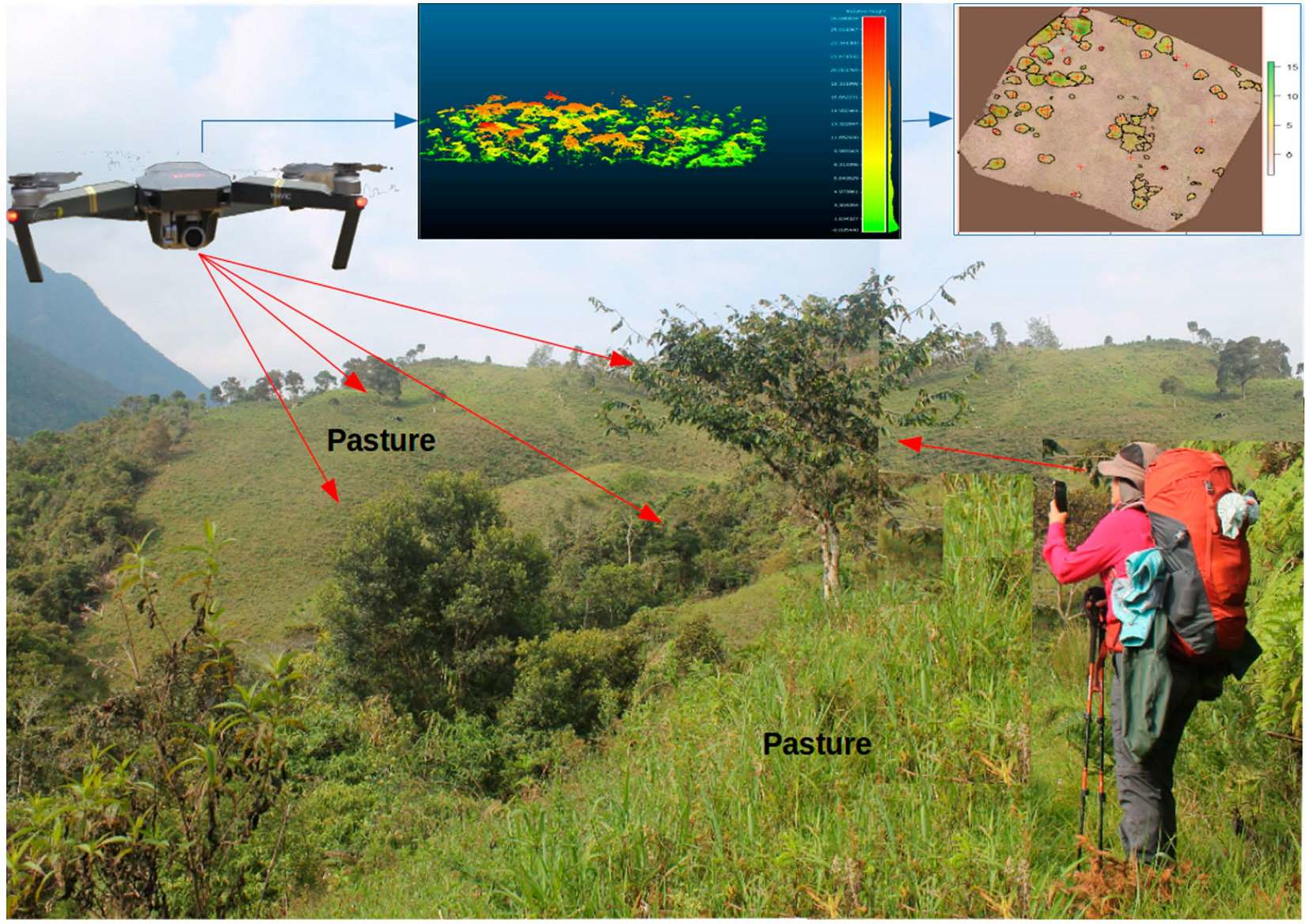
The performance of surveys by small unoccupied aerial systems (UASs) can be an alternative approach to overcome constraints relating to spatial and temporal scales, especially in developing countries, where research funds can be a limiting factor [18]. The use of UASs for aerial surveys in ecological studies has been demonstrated to: (a) be a good option in study areas with difficult access [19], (b) reduce the time and labor used in traditional surveys [20], (c) cover larger areas [21], and (d) allow high temporal resolution [22]. Information generated from UAS surveys depends on the type of sensors used (RGB, NIR (near infrared), thermal, or LiDAR). Most commercial UASs have an integrated RGB camera as a default option, which makes them feasible, inexpensive, and practical options for aerial surveys in developing countries. Although LiDAR and NIR sensors provide a broader range of information with which to assess forest canopy characteristics, the development of open-source photogrammetry software and algorithms in recent years has made it possible to extract information from RGB sensors to assess forest characteristics (such as tree height and crown diameter), with results similar to those obtained from LiDAR surveys [23], with considerably lower costs. Several studies using UASs to assess forest characteristics have been published [24,25,26,27,28], but few have focused on the potential for studying SPS [29,30]. The use of photogrammetry to assess tree characteristics on SPS follows the same principles as in forested areas. The main difference between forest and pasture-dominated areas is the extent of the canopy gaps, which, by definition, are considerably larger in pasture areas, thus improving ground-truth detection and digital-terrain-model (DTM) creation using structure-from-motion (SfM) workflows [27]. The accuracy of tree-characteristics estimates depends on terrain conditions, and remains a challenge in areas with steep slopes [31]; however, even in even terrain, the accuracy depends on the tree stands’ density and the methods used to calculate their characteristics [30].
When studying trees in agricultural landscapes, either as agroforestry or silvopastoral systems, the detection of individual trees becomes a key part of the analysis as, with the usual low tree density, it is important to recognize every individual. Methods to detect trees can rely on local maxima methods [24,25], object-based classification [32], or, as shown more recently, using neural networks with RGB imagery [33]. Nevertheless, it can still be considered a challenge, especially in developing regions, where some methods, such as object-based classification, are mainly performed by paid software, while local-maxima methods have mostly been applied using LiDAR-derived data. Nonetheless, UAS surveys represent an opportunity to study SPS and address other issues that have not been studied enough, such as spatial arrangements at larger spatial extents. While more sophisticated hardware may provide more accurate results, we used inexpensive and readily available hardware to test whether the method could be used in developing countries, where resources are more limited. In this study, we propose an approach that combines field-level techniques (plot measurements) with remote-sensing information (UAS photogrammetry) to study SPS characteristics. The overall aim of the study was to assess the suitability of UAS surveys to estimate aboveground biomass on SPS. To achieve this, we: (1) compared the best parameter combination for point-cloud processing and classification, by evaluating the canopy-height-model differences against field measurements; (2) assessed the performance of individual tree detection derived from canopy-height models vs. visual identification in ortho-mosaic images; and (3) assessed the tree spatial arrangements and distribution of SPS.

2. Materials and Methods

2.1. Study Sites

This research was conducted between May and December 2018 on 101 livestock farms in Ecuador, as part of the Climate Smart Livestock project [34]. In total, 43 farms from the Amazon region and 58 in the Coastal region of Ecuador were surveyed. For this study, 5 farms per region were randomly selected. Farms were distributed in an altitude range from 8 to 426 m asl and 451 to 2000 m asl, in the coastal (C1–C5) and Amazon (A1–A5) regions, respectively (Figure 1). The main activity on the studied farms was cattle-livestock production, but most of the farms also dedicated land to other economic activities, such as perennial crops, annual crops, other livestock, or conservation.
To achieve the proposed aims of this study, we divided the work into three stages (Figure 2).First, combining traditional forest field measurements with UAS surveys, we collected tree characteristic information (a). Secondly, we transformed the 2D data (individual photos) into landscape information in 2D (orthomosaic) and 3D (digital surface model (DSM), point cloud), which is explained in Section b in Figure 2. Finally, we used the products of Section b to estimate tree characteristics and compare them against measured values (Figure 2c).

2.2. Plot Delimitation and Tree Inventory

Farmers were asked to identify grazing areas that were representative of their farms [35]. Once the areas were identified, two 1-hectare square plots were installed. Plot corners were marked with a plastic sheet to make them visible from the UAS survey, and geographical coordinates were collected with a Garmin GPS50 GPS with an accuracy of +/− 5 m. Plots were established with a minimum distance of 200 m between the plot centers. Inside each square plot, a circular plot with radius R = 17.84 m was installed; the center was marked with a plastic sheet and geo-referenced. The circular plots were used to capture the diversity of tree arrangements in the pasture areas. Forest and secondary forest patches were avoided at the time of circular-plot installation, due to the lack of grazing (Figure 2a). In the circular plots, trees with a diameter at breast height (DBH) ≥ 0.10 m and height ≥ 2 m were measured and recorded. Total height, commercial height, and crown diameter was measured, and the trees’ geographical coordinates were also recorded.

2.3. UAS Missions and Image Processing

UAS surveys were performed using a DJI Mavic Pro quadcopter (DJI Inc, Shenzen, China), equipped with a 12-megapixel, 35-millimeter-focal-length RGB camera. A flying area of 1.56 ha (125 × 125 m), covering the square plots, was designed using the Pix4Dcapture application (Pix4Dcapture 4.3; Pix4D SA, Lausanne, Switzerland), using tablet device with an Android operating system. In the Pix4D application, flights were set to 80% forward and 72% side overlap, flying height was set to 60 m, and camera pitch was set to 90° heading forward. Mission-camera parameters were as follows: focal length, 4.695; image height, 3000; image width, 4000; minimum photo interval, 2.0; sensor width, 6.17. The surveyed area was set to cover a bigger area than the square plot (Figure 2a), in order to ensure sufficient photographs were taken for modeling of the surveyed area. The durations of the flight missions were approximately 8 min, during which between 80 and 150 pictures were obtained, following a grid flight path, which is illustrated in Figure 2a. Images were automatically geotagged with the UAS-incorporated GPS. As a preliminary step, poor-quality images (featuring blurriness, or a bad photograph ensemble) were manually selected by the operator and discarded. The remaining pictures were included in the photogrammetric analysis, which was performed using Web Open Drone Map software (OpenDroneMap, https://github.com/OpenDroneMap/ODM/blob/master/README.md, 10 April 2022) [36]. For the point-cloud creation, three processing parameters were selected: Web Open Drone Map default settings (def), and two alternative versions that differed from the default settings, except for the resolution parameters, which were increased-resolution (par1) and high-resolution (hres) settings (Table 1). Processing parameters are characterized in Appendix A. A digital-surface model (DSM), an orthomosaic (OM), and an unclassified dense point cloud (PC) were obtained from photogrammetric analysis (Figure 2b). Due to the time spent on processing under hres, the PC was not considered in the point-cloud-classification process.

2.4. Point-Cloud Classification and Canopy-Height-Model Building

A canopy-height model (CHM) is an object containing the height of the vegetation aboveground and is calculated as the difference between a DSM and a digital terrain model (DTM). Although the software allows a DTM to be obtained as a primary output of the photogrammetric analysis, site characteristics and image quality can produce PC misclassification, which can have an impact on the CHM and, subsequently, on the estimation of trees and forest characteristics. To reduce the misclassification issues, classification was controlled and performed in CloudCompare v2.11 software [37], where PCs were imported. As a first step, points that were visually identified as outliers (below the PC surface or extremely distant from the PC top) were removed [38], and, later, the PC classification was performed using the Cloth Simulation Filter (CSF) plugin [38], as explained in Figure 3a. The algorithm used in the CSF inverts the PC and simulates a rigid cloth on the inverted surface. The nearest points to the surface drawn by the cloth are classified as ground points, and the remaining points are classified as non-ground points (PCng). The CSF has four sets of parameters that can be selected, according to the project characteristics. The scene parameter allows cloth rigidness to be selected from the following options: very rigid (flat), rigid (relief), and soft (steep slope). The slope-processing parameter (yes–no) allows the consideration of terraced slopes. The underlying process for cloth resolution and classification threshold parameters can be found in Zhang et al. (2016). In this study, we evaluated three cloth resolutions (0.2, 0.5, and 1.0) and three classification threshold sizes (0.2, 0.5, and 1.0). Since the best combination of parameters was unknown for each of the plot characteristics, an exploratory combination of all the parameters was performed, except for scene, where an operator visually identified the plot characteristics and selected one or two of the options. Between 18 and 36 classified PCs were produced for every set of PCs; combinations of CSF classification parameters used for each plot are specified in Table 2.
Trees or other non-ground structures, identified in the original PC, are shown as a lack of points in the ground point cloud (Figure 3a). To fill these gaps, the raster tool was used with the average scalar field interpolation method in the CloudCompare software. A filled-ground PC (PCfg) was generated as the result of the rasterization process, which can be interpreted as a DTM for the study area. Finally, a CHM was computed as the difference between PCng and PCfg, using the 2.5D volume tool and exported as a Geotiff file.

2.5. Individual Tree Detection and Tree Characteristics

CHMs were imported into the R environment [39], where, first, we tested whether a smoothing process could improve tree detection. Smoothing was performed using the CHMsmooting function, from the rLiDAR package [40], using a median filter and three pixel sizes (sm3 = 3 × 3; sm5 = 5 × 5; sm7 = 7 × 7), which were compared against a non-smoothed CHM (sm0) version [24]. For individual tree detection, the local-maxima algorithm, with the variable-window-filter function (vwf) from the ForestTools package [41] was used, with a minimum height of 2 m. Five window sizes (w1 = 1, w2 = 2, w3 = 3, w4 = 4, w5 = 5) were tested to explore the differences in the individual tree detection. Subsequently, the marker-controlled watershed segmentation function, with a minimum height of 1.5 m, was used to calculate crown height, diameter, and area for every identified tree. The entire process can be seen in Figure 3b. As a result, for every combination of smoothing level and window size applied to a CHM, a polygon shapefile with information about individual tree geographic coordinates, height (hm), crown area (tcm), and crown diameter (cdm) was obtained.
To compare the results from the photogrammetric analysis and field measurements, the shapefiles from the previous steps were masked into the circular plot area, containing information about tree characteristics that were measured on the field (Figure 2a). First, we selected only the models that identified the exact number of trees, as measured on the circular plots. Subsequently, root mean square error (RMSE) was calculated to assess the difference in tree height and crown diameter between field measurements and values obtained from the UAS. For each parameter, the 5 outputs with smallest RMSEs were selected.

2.6. Tree Density

Individual tree-detection spatial accuracy was evaluated using a methodology similar to [24], which consists of the comparison between modelled and independent visual assessment of trees on the UAS-derived ortho-mosaic. Ten squares of 400 m2 were randomly distributed on each farm, and, in these, an operator visually identified individual trees and generated a points shapefile containing tree coordinates for each validation square, using QGIS software (QGIS.ORG, Bern, Switzerland) (Figure 4).
Tree density was merged with validation squares and later imported to the R environment, where the validation squares were used to crop the tree-points shapefile. A dataframe containing the number of observed trees and modeled trees was obtained. Density difference (Difdensity) was calculated as the average absolute (Abs) difference between observed (Obs) and modeled trees (Mod), expressed in terms of percentage (Equation (1)). The parameter combination that delivered the five lowest Difdensity values was selected.
D i f d e n s i t y i j = i j ( | ( ( O b s i M o d i ) × 100 O b s i ) | ) 10

2.7. Cloud Processing, Point-Cloud Classification, and Individual-Tree-Detection Selection Parameters

The ideal parameter combination for tree height, crown diameter, and tree density was identified using frequency tables from the combinations that presented 5 lowest RMSEs for each category. For each cloud-processing level (odm), cloud-classification variable (scene, slope processing, cloth resolution, classification threshold) and individual tree-detection parameter (smoothing, window size), the relative frequency was calculated, with values ranging from 0–1. Values close to 1 showed a higher frequency of a given level in a variable, and if values were closer to 0, then there was not predominance of a given level in the studied variable. Values between 0.76–1 were considered to be in strong agreement and are shown in green, whilst a value between 0.51 and 0.75 was considered to be in medium agreement and is shown in yellow. Values equal to or lower than 0.50 were considered to be in weak agreement and are shown in red.

2.8. Tree Spatial Arrangements

Tree spatial arrangements were assessed using the best combination of parameters for tree height, crown diameter and tree density in the previous section. Prior to the spatial analysis, shapefiles containing tree location were cropped into a smaller area, to avoid border effects on individual tree identification. A distance-based approach to cluster identification was used, in which clusters are formed when the distance between at least two trees is less than a given distance d [42]. A distance d = 6 m was used as the criterion for cluster definition [43]. Since spatial coordinates for every modeled tree were known, the buffer function from the raster package in R was used [44] to create a buffer area of radius = d around each tree, as shown in Figure 4. Next, the overlapping buffer areas were merged into a single polygon, allowing the spatial arrangements to be identified. Spatial arrangements were classified as scattered trees (individual trees with distance >6 m to the nearest neighbor) and clumps (two or more trees with a minimum distance ≤6 m between trees) [43]. Clumps were subclassified into small (2–9 trees), medium (10–19 trees), and large clumps (>20 trees). Results are presented in terms of percentage of trees under these category arrangements.

2.9. Aboveground Biomass

Aboveground biomass from measured values at the circular plot level was calculated using Equation (2) [45]. This equation requires the wood-density parameter, which was retrieved at genus level from the Global Wood Density Database [46] using the getWoodDensity function from the BIOMASS package in R [47]. When genus information was not available, wood density was estimated as the average density at site level (Chave_wdsite) [48] and family level (Chave_wdfamily). Biomass was estimated from measured values, using Equation (3), proposed by [49], which was developed for remote-sensing imagery; the equation relies on tree-height and crown-diameter parameters. The use of Equation (3) with measured values was completed to estimate the differences in measured values separately from the values obtained from the UAS imagery. Using the tree-height and crown-diameter information derived from the CHM, Equation (3) was used to estimate biomass and compared against values obtained in the field. Finally, the share of above-ground biomass was calculated for each spatial-arrangement category.
A G B C h a v e = 0.0673 × ( W D × H × D 2 ) 0.976
A G B J u c k e r = ( 0.016 + 0.093 ) × ( H × C D ) ( 2.013 0.223 ) × e x p [ 0.204 2 2 ]

3. Results

3.1. Site Characteristics and Tree Inventory Results

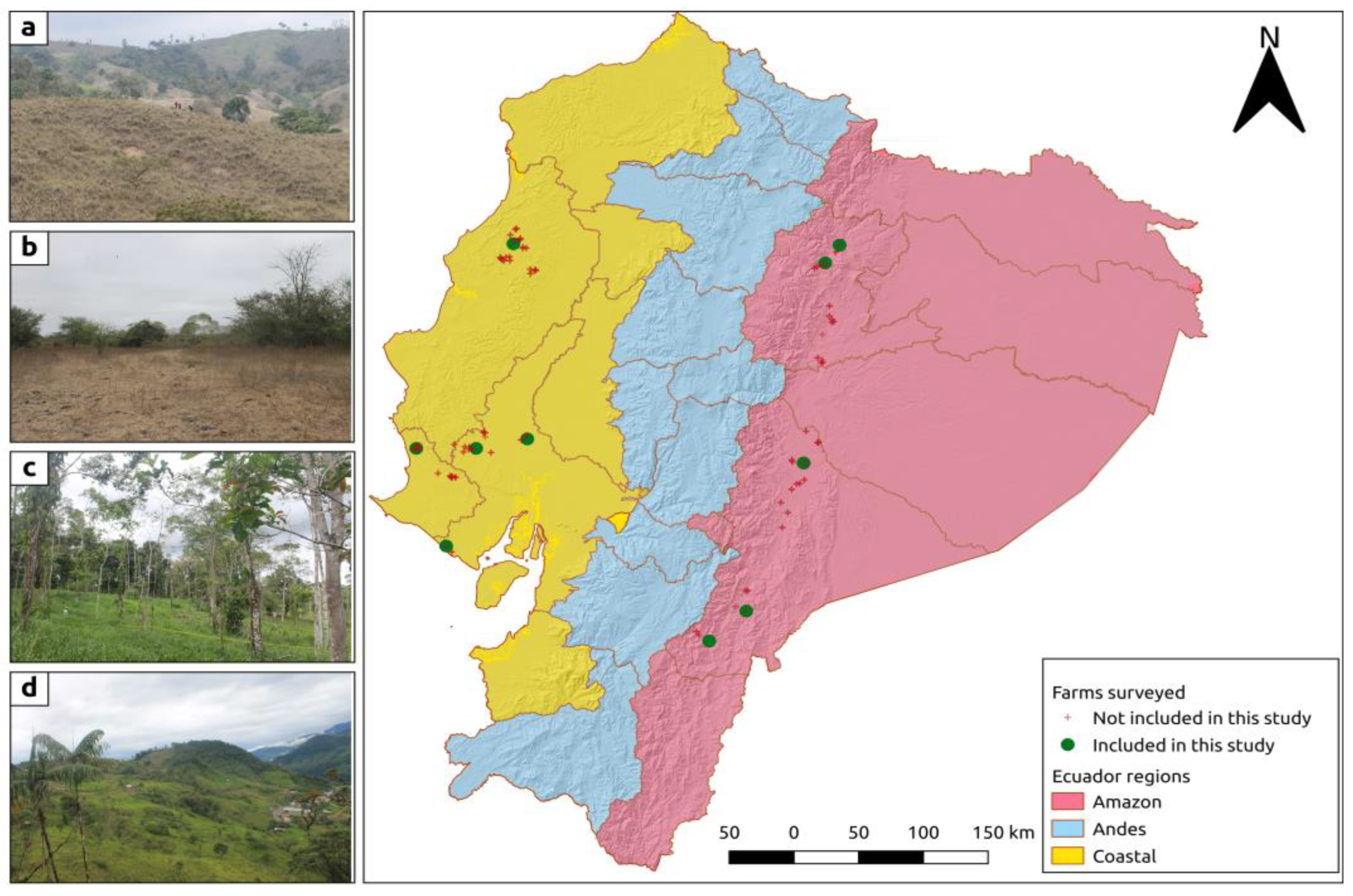
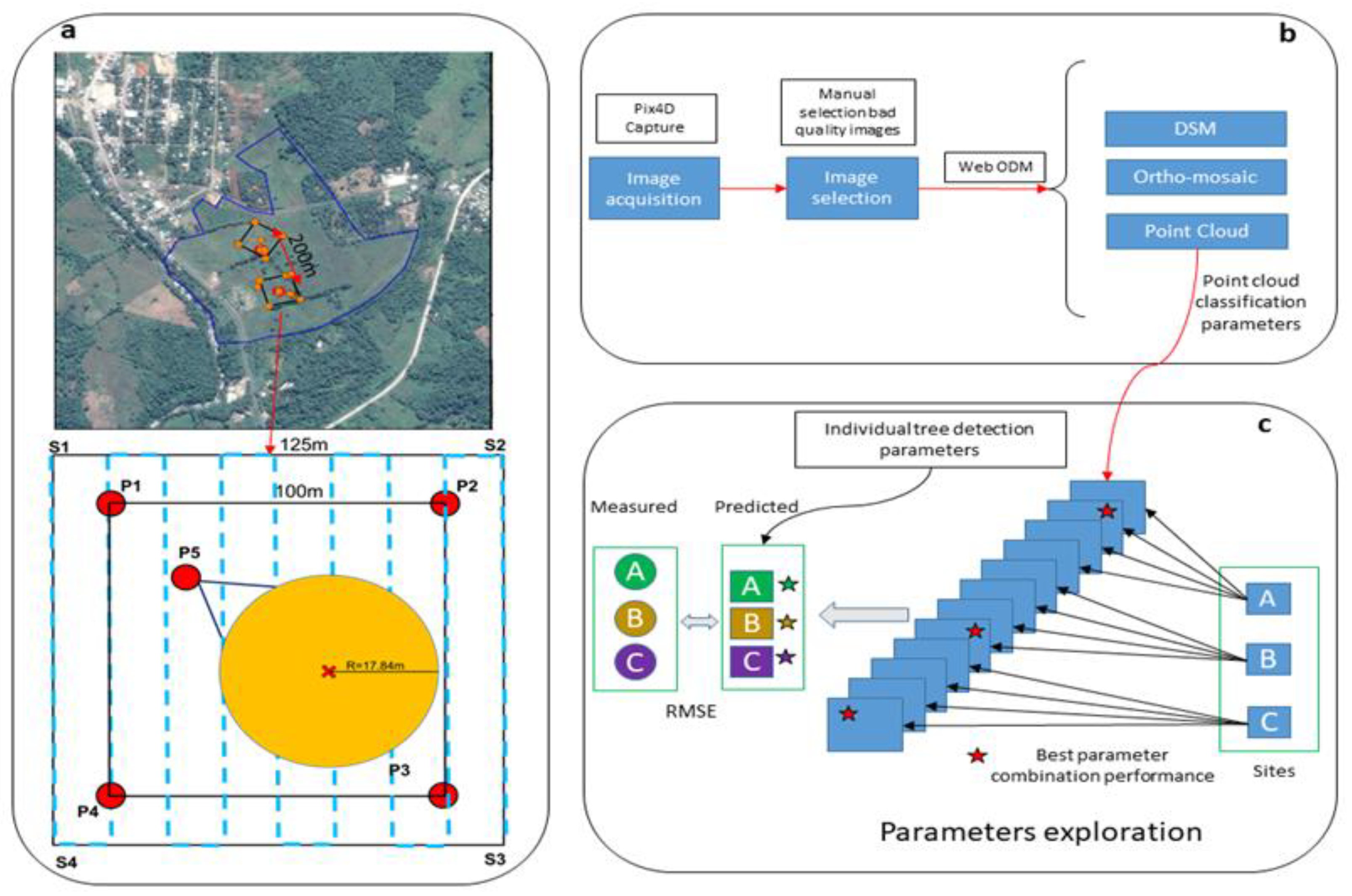
The circular plot installation (0.1 ha) and tree measurements on the pasture areas each took 2–5 h, depending on the number of trees, using teams of four people. For the UAS survey, a team of two people and 45–60 min were needed for every 1.56-hectare plot. Since the surveys were performed on areas that farmers use for cattle grazing, open areas covered with grass species were dominant. The terrain slopes varied between the plots, but, in general, irregular terrains with slopes ≥ 20% were found in the Amazon region (plots A1, A2, A3, and A5), whilst in the coastal region, the slopes ranged between 4 and 16% in four plots; only in plot C4 was this value above 20% (Appendix B). In total, 58 trees were surveyed, with a minimum of 1 and a maximum of 17 trees per plot. The tree heights ranged from 2.4 to 21 m, and the crown diameters ranged from 2.5 to 15.6 m.

3.2. Cloud-Point Creation

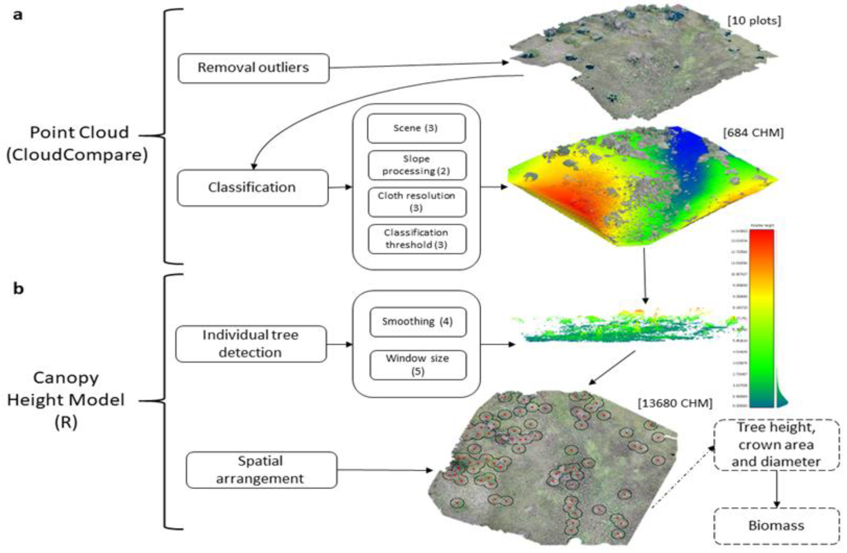
The differences in the point-cloud building settings had an impact on the processing time, point-cloud size, and percentage of discarded points, with par1 settings using more processing time, displaying smaller point-cloud sizes and removing fewer points than the def characteristics (SI2). The processing time for all the plots was 12:02:22 h under default characteristics, 16:49:56 h for par1 settings, and 34:16:45 h for high-resolution settings. For the point-cloud size, the par1 point cloud had, on average, 4,281,057 fewer points than the default characteristics, whilst the high resolution had 32,430,874 more points. The percentage of points identified as outliers and removed varied from 0.32, 0.059, and 0.20% for the default, par1, and high-resolution settings, respectively. Due to the processing time needed for the high resolution, the next steps considered only the def and par1 outputs. From the def and par1 settings, 13,680 outputs with individual tree detection were generated. Of these, only 5078 detected an exact number of trees inside the circular-plot validation, making them suitable for assessing differences among measured values. Due to the differences in site characteristics, the point-cloud classification and individual tree-detection parameter combination were expected to vary between plots, but also to show similarities in plots with similar characteristics. The similarities between the plots are discussed in the Discussion section.

3.3. Canopy-Height-Model Validation

For the calculation of the biomass from the field measurements, in which the correct measurement of the tree parameters resulted in more robust estimations, the tree parameters obtained from the UAS surveys needed to be validated against field measurements to prove their usefulness on biomass estimations. The tree heights and crown diameters were compared against the field measurements to identify possible sources of error in the final biomass estimates.

3.3.1. Tree-Height Differences

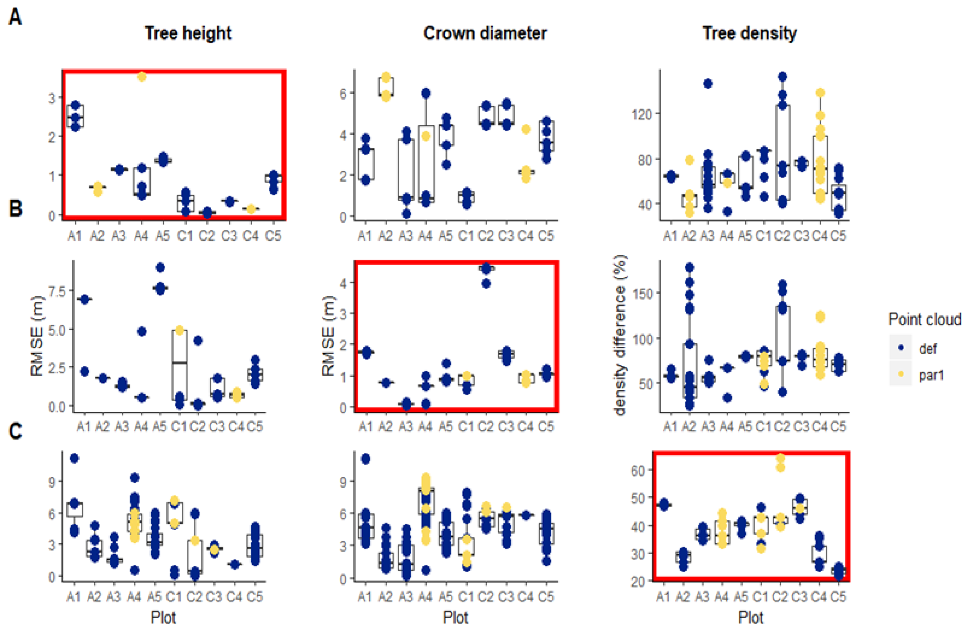
The RMSEs of the best models ranged from 0.49 to 3.53 m and 0.01 to 1.01 m in the Amazon and the Coastal regions, respectively (Figure 5a). The point-cloud-building, classification, and individual tree-detection parameters did not significantly influence the estimates of tree height when analyzed separately. The relative frequencies for each parameter level for the tree height sand crown diameters are presented in Table 2. The point-cloud building specifications (ODM) resulted in high agreement (>0.75) in all the plots, with 80% of the plots showing lower RMSE under the def settings in the Web Open Drone Map software, whilst in the plots A2 and C4, the best results were found using the par1 specifications. With the point-cloud classification parameters, only the cloth resolution (CLR) and classification threshold (CTR) presented a high agreement in more than 50% of the plots, with a CLR size of 1 for 70% of the plots and CTR of 0.2 for 50% of the plots. Meanwhile, for the scene and slope processing parameters, medium agreement within plots was found in 50% and 60% of the plots, respectively. The flat scenes performed better for the plots in the Coastal region, whereas the steep slope and relief scenes were predominant in the plots located in the Amazon region. In 60% of the farms, the tree heights were estimated better without slope processing, whilst a cloth resolution size of 1 and a classification threshold of 0.2 were the most common settings for at least 50% of the plots. The parameters for individual tree detection reached strong agreement in 40% of the farms for window-filter size, and medium agreement in 50% of the farms for smoothing-window size. Only window-filter sizes 1 and 5 presented strong agreement, and the smoothing-window process presented strong agreement at sizes 0, 3, and 5.

3.3.2. Crown Diameter Differences

The RMSEs for the best models ranged from 0.04 to 1.77 m and from 0.53 to 4.47 m for the Amazon and Coastal regions, respectively (Figure 5B). Similarly to the height estimation, the ODM parameter presented strong agreement in 90% of the plots, among which default characteristics for point-cloud building were present in 80% (Table 3). For the point-cloud-classification parameters, scene resulted in high agreement in 40% of the farms, whilst the other 60% reached only medium agreement. The steep slope was the most common scene for the plots in the Amazon region and flat was the most common for the Coastal region. Avoiding slope processing presented the best results in 70% of the farms, with strong agreement in 50% of them. Cloth-resolution sizes of 0.2 and 1 were present in 40 and 50% of the plots, respectively, and showed strong agreement in only three plots. The classification threshold reached strong agreement in 50% of the plots, with a size of 1 present in 40% of the plots, followed by 0.5 in 30% of plots, and 0.2 in only two plots. The window-filter size resulted in strong agreement in only one plot and medium agreement in one, but with a size of 5. The smoothing process resulted in agreement in 50% of the plots, with size 5 present in 30% of the plots, and size 3 in 20%.

3.4. Tree-Density Assessment

The tree-density differences ranged from 25 to 48% and from 21.85 to 64.28% in the Amazon and Coastal regions, respectively (Figure 5C). The point-cloud-building specifications showed strong agreement in 70% of the plots for the default characteristics, and medium agreement was found for three plots, with one def and two par1 characteristics (Table 4). For the cloud-classification parameters, scene resulted in strong agreement in 40% of the plots, with two flat and two s.slop; meanwhile, 50% of the farms resulted in medium agreement, with three plots with a relief scene, and one with a flat and steep slope. For the slope processing, medium agreement was found in 80% of the plots, with 50% of the plots resulting in better tree-density estimates with slope processing and the other 50% without it. Cloth resolution resulted in strong agreement in 50% of the plots, whilst the other 30% showed medium agreement, and 20% showed low agreement. The classification threshold resulted in medium agreement for 50% of the plots, and strong agreement was found in only one plot. The most common cloth-resolution size was 0.5 (3 plots), followed by 0.2, and 1, with one plot each. Strong agreement was absent in the window-size-filter parameter, while medium agreement was found only in four plots, with size 2 present in three of them. No-smoothing showed medium and strong agreement in two plots.
Using the best models for tree height, crown diameter, and tree density, the average relative frequency was calculated for an ideal combination of parameters that could help to improve the estimations. The relative-frequency values were averaged for every parameter level. The apparent optimum model combination showed a strong agreement for default point-cloud building on 70% of the plots, whilst in the other 30%, there was medium agreement, with one plot with par1 settings. The point-cloud classification parameters gave medium agreement for scene (70% of plots), slope processing (90% of plots), and cloth resolution (60% of the plots). For the tree-detection parameters, the window-size filter resulted in low agreement for 90% of the plots and medium agreement for one plot. The smoothing-processing window resulted in medium agreement for 50% of the plots and low agreement for the other 50%.

3.5. Spatial Arrangements

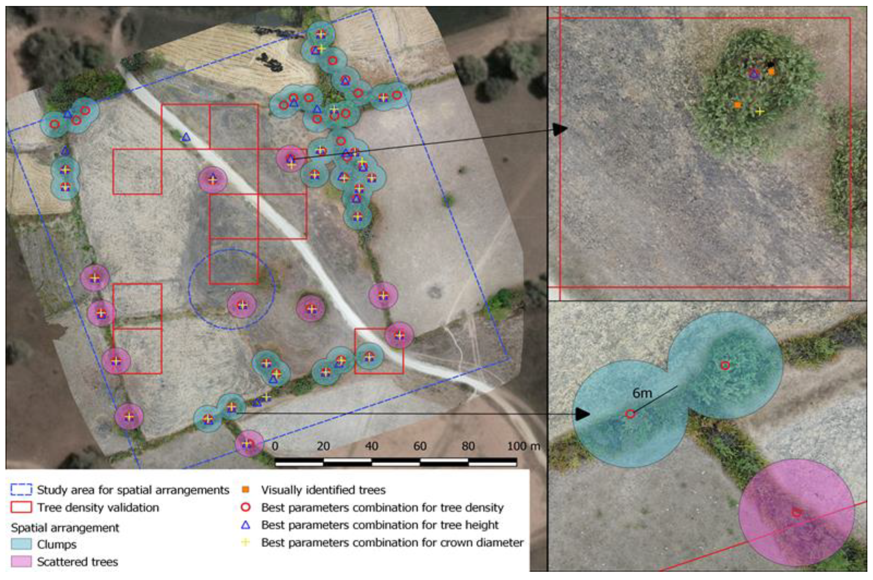
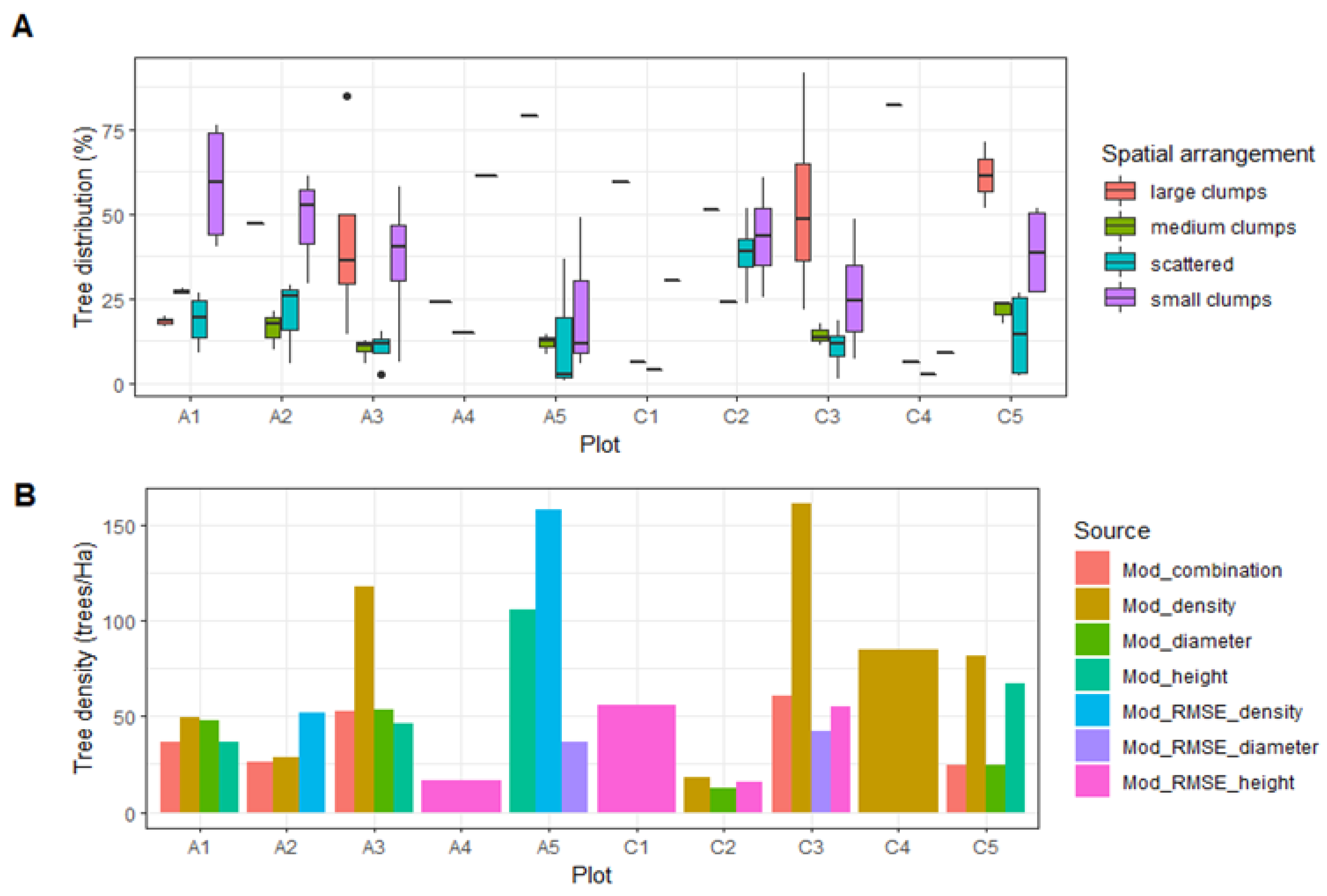
The methodology proved to be useful for identifying the spatial arrangements of trees in livestock landscapes. Although the number of individual trees detected was influenced by a combination of parameters (Figure 6B), the average tree distribution for was used to determine the spatial arrangement. On the plots located in the Amazon region, with the exception of A5, the majority of the trees were grouped in small clumps, whilst in the plots located on the Coastal region, the majority of the trees were grouped in large clumps, as seen in Figure 6A. On plot A5, most of the trees were grouped in large clumps. The number of trees identified in the square plots varied depending on the parameter-combination selection criteria; in plots A1, A3, C2, C3, and C5, the parameter-combination selection that focused on tree-density validation resulted in a higher number of trees, whilst in plots A2 and A5, the parameter combination that showed the lowest RMSE for tree density identified a higher number of trees in comparison with the other parameter-combination criteria. For plots A4, C1, and C4, only one parameter-combination criterion identified the exact number of trees inside the circular plots.

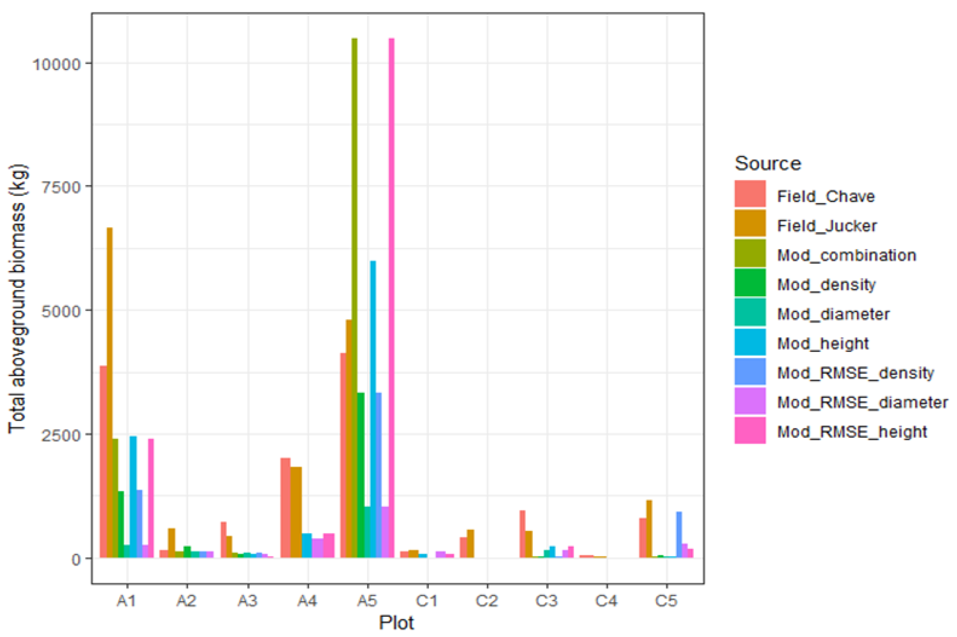
3.6. Biomass Estimation

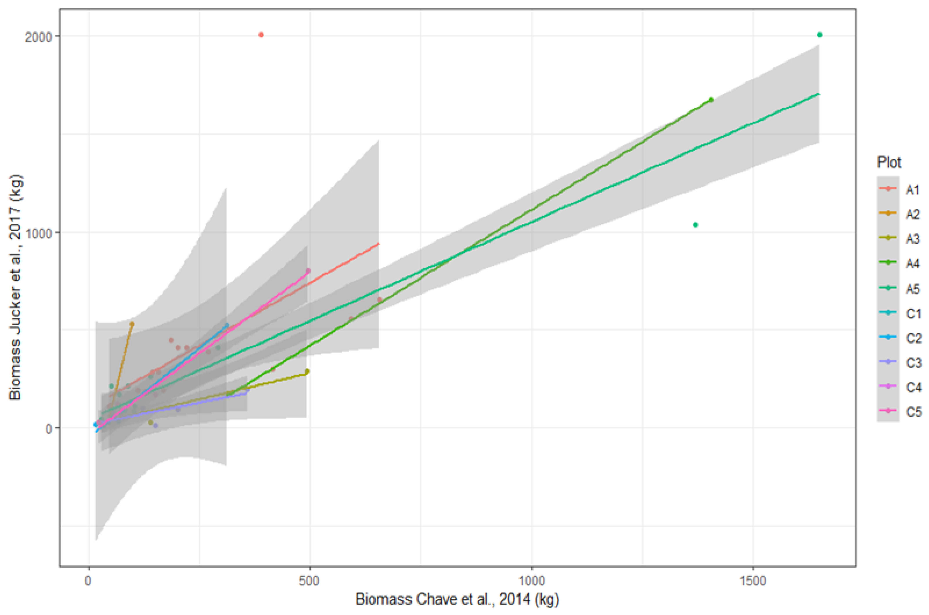
With information obtained from the field measurements, the difference in biomass estimates as the result of the equation selection was compared. The biomass calculated using Equation (3) showed higher mean values compared with Equation (2) in seven plots (Figure 7), although the standard deviations showed similar values. The average biomass estimated with Equation (3) presented higher values in plots A1, A2, A4, A5, C2, and C5, whilst in A3, C3, and C4, the Equation (2) estimates were higher.
When comparing the biomass estimates from the field measurements against those obtained from the UAS survey, the results and best parameter combinations varied according to the plot. This was expected, since the performance and reliability of UAS surveys is greatly influenced by the site conditions; consequently, the point-cloud classification and individual tree-detection parameters varied between the sites.
The sum of the biomass per plot allows us to compare the differences between parameter combinations and biomass obtained from measured values. When comparing against biomass estimated using Equation (2), the best estimates of biomass for plots A2 (average combination), A5 (lowest RMSE for tree density), C1 (crown diameter), and C5 (tree density) were 127.96, 3324.99, 131.28, and 929.09 kg, respectively, with these values differing from the measured values by less than 25% (Figure 8). In these plots, the biomass estimated using Equation (2) was lower than that estimated with Equation (3). In plot A1, with the parameter combination for tree height, a biomass estimate of 2446.34 kg was obtained, which was 36% lower than that estimated using Equation (2). In plots A3, A4, C2, C3, and C4, the biomass values estimated from the UAS imagery were 88.46, 490.40, 2.26, 219.76, and 0.028289 kg, respectively. These values differed by more than 75% from the values estimated from the measured tree characteristics on the field using Equation (2). The parameter combination used in these plots was crown diameter (A3, C2), the lowest RMSE for tree height (A4, C3), and tree density (C4).
When comparing the biomass estimates derived from the UAS metrics against those obtained using the measured values and Equation (3), for plots A5, C1, and C5, the parameter combination for tree height, the lowest RMSE for crown diameter, and the lowest RMSE for tree density resulted in differences of less than 25% compared to the measured values. For the rest of the plots, the differences were greater than 50%.

4. Discussion

Traditionally, the study of trees on pasture areas has been performed using measurement plots, the results from which are then extrapolated to the entire pasture area on the studied farms or region. At larger scales, other approaches have used tree coverage information (in terms of percentage), which are superimposed onto the pasture categories on land-cover maps [50]. While both approaches have improved the understanding of the contribution of trees on pasture areas to carbon budgets, neither adequately captures the heterogeneity within and between farms or landscapes. The use of UASs can be used to complement traditional field measurements and, possibly, to provide an intermediate step between ground- and satellite-based remote sensing.
In the past, only a few studies explored the use of UASs for the study of tree characteristics in livestock landscapes [29,30]. In this paper, a new methodology is proposed for using UAS surveys for the assessment of woody vegetation in silvopastoral systems. The methodology relies mainly on open-source (OS) software, making it more accessible in developing countries, where research funding can be scarce [18,51]. Although commercial software dominates the field, an increasing number of studies use open source software [52,53,54,55]. In terms of the processing steps required, in general, increasing the resolution of the photogrammetric analysis resulted in an increase in total processing time of 04:47:34 h from the def to the par1 and 22:14:23 h from the def to the hres settings. Although the proportion of removed points was lower under par1 and high resolution, the best results were found under default characteristics (Table 4 and Table 5), making it unnecessary to invest more time, since no improvement could be obtained in the desired outputs. When assessing the performance of different photogrammetry OS software, the authors of [55] found that WODM default settings performed better in comparison with other OS software, but were less accurate than commercial settings. The plots included in this study differed in tree density and terrain characteristics (Appendix B), which ultimately had an effect on the ability to correctly identify tree characteristics and biomass estimates (Figure 8). For example, in plot C4, field measurements recorded only one tree 3.1 m in height, probably causing a low point density in the point cloud and, subsequently, an inability to identify it from the UAV survey data.

4.1. Tree Parameters and Biomass Estimation

Most of the work using UAS for the study of forest characteristics relies either on high-resolution DTM from LiDAR surveys [26,56] or high-accuracy GPS [28,57] to calculate CHM from DTM. This approach relies entirely on the performance of point-cloud-classification algorithms to correctly differentiate ground from non-ground structures. The authors of [23] tested the use of UAS-independent metrics to predict forest-growing stocks in flat forest areas in Norway and Italy. Their findings suggest that it is possible to rely only on UAS-DTM-independent metrics to estimate ground-stand volume, with RMSE values similar to those obtained when using a high-resolution DTM. Site conditions, such as terrain slope and tree cover, have an influence on point-cloud-classification performance, although the authors of [30] suggest that tree coverage is more important for accurate DTM creation. In this study, three of the four plots that had a RMSE between 1.14 and 2.5 m (≥10% relative RMSE) were located in areas with a slope of between 20 and 29°. With the exception of plot A1, the results of this research include lower RMSE values than those reported by the authors of [28] (1.45 m), who used high-accuracy GPS in a study on restoration areas with terrain slopes between 15 and 30° in Costa Rica, and the values reported by [26,56] on forest areas with closed canopies in Japan and Sumatra, respectively. The error associated with tree-height estimation is also influenced by the height of the studied trees; the authors of [29] reported an RMSE of 3.8 m in trees with heights equal to or lower than 1 m, with a consistent decrease until 1.5 m for trees 2 m in height, and a 0.9-meter RMSE for trees with a height of 8 m. Since this study only considered trees with heights equal to or above 2 m, with the exception of plot A1, the results showed a similar performance. When analyzing the performance of UAS-derived CHM models in estimating crown diameter, the worst performance was found for plot C2, with an average RMSE of 4.43 m, followed by plots A1, C3, and C5, with 1.74, 1.66, and 1.05 m, respectively. In the rest of the plots, the RMSE values varied between 0.1 and 1 m. The authors of [58] reported RMSE values of 0.73 m for crown width derived from photogrammetry analysis in a eucalyptus plantation in Australia.
Most allometric equations use tree height and DBH as the main parameters to estimate tree biomass [45]. Nevertheless, it is difficult to obtain DBH from traditional UAS surveys. Whilst previous work has assessed the suitability of using UAS for a full reconstruction of trees [53], this could require different flying parameters, requiring more time and making the UAS survey less efficient. The authors of [48] proposed a specific equation for using remote-sensing data in tropical forests, which was proven to result in more reliable biomass estimates when compared with field measurements [48]. Although several papers have reported a relationship between crown width and DBH [48,55], this relationship might be different in trees in agricultural landscapes, because growing conditions differ from those in natural forests, and/or because management practices, such as pruning and foraging, modify crown development. Hence, the crown–DBH relationship was altered, which may have exerted an impact on the final biomass estimates. For example, the authors of [30] reported a low R2 for equations using crown diameter as a predictor of DBH on Tectona grandis trees in SPS in Costa Rica. Although biomass estimates present differences in comparison to biomass estimates derived from field measurements, by assessing the error magnitude, these estimates can be useful for reporting carbon stocks in SPS at larger spatial extents.

4.2. Tree-Density Assessment

The preliminary tests of the method for individual tree detection showed that smaller window sizes produced more trees per plot, in some cases splitting large trees into several small trees. Since the nature of this work was exploratory, the range of the detected trees varied across the parameter combinations. Nevertheless, the relative frequency values presented medium agreement for only four plots, with window sizes of 5 for plot A1 and window sizes of 2 for plots A5, C3, and C5. The results suggest that while window size can be an important predictor for correct tree-density assessment, the point-cloud-building and classification parameters played a larger role in the tree-density estimation. The authors of [29] reported that the proportion of trees found was dependent on the tree height, with trees with heights below 4 m displaying identification rates below 75%, which increased to 90% for trees taller than 4 m. The authors of [24], using a watershed algorithm, identified 93.8% of the trees in areas with a density of 150 to 325 trees/ha. Due to the quantity of output from the parameter combination (13,680), these results did not consider omission and commission errors separately for every plot; instead, these errors were integrated into a comprehensible and easy-to-calculate index, which represents the percentage difference with visually identified trees, independent of the number of trees in each subplot.

4.3. Spatial Arrangement Assessment

Spatial arrangements have been identified from field measurements by other authors [59], but the problems with these are the same as those reported for tree measurements, i.e., the elevated costs associated with identifying all of the arrangements. One of the negative effects of trees in pastures, as perceived by farmers [60], is the shades that trees cause, and their detrimental effect on grass biomass production [61]. UAS surveys in livestock landscapes could allow areas with excess shade to be identified and, further, allow the distribution of trees to be improved, mitigating the negative effects and increasing the positive effects. The methodology proved useful for identifying tree arrangements on pasture areas, although, in this study, we only classified the arrangements into four categories. Analyzing the clump characteristics (length and width) can improve the classification and contribute to the inference of the functionality of spatial arrangements, depending on their locations on farms.

5. Conclusions

The methodology described in this study provides a tractable and economical approach to studying the presence of trees, as well as their arrangements, spatial distributions, and individual characteristics (such as height and crown diameter) in livestock landscapes, which can be used to estimate ecosystem services, such as carbon storage. Point-cloud classification remains a challenge for improved DTM generation, especially in areas with highly irregular terrain. In this study, tree species were identified with field observations at circular plot level, but this information was not considered at UAS survey level. Thus, the biomass estimates used a generic equation for the entire plot. Accounting for all the species at landscape level includes the same problems as measuring trees at that spatial extent. To overcome this difficulty, one option is the use of orthomosaics for species identification [33,62]. Although uncertainty over UAS-derived biomass estimates is still high, the possibility of allocating those estimates spatially, across spatial arrangements and landscapes, can be seen as an improvement in understanding the factors influencing carbon stocks in livestock or agricultural landscapes. The generation of orthomosaics from UAS surveys can also be useful for communicating the importance of tree presence in livestock landscapes to farmers and other stakeholders. The visual assessment of the lack/abundance of trees in the landscape might open up opportunities for reflection and discussion about the role of trees on farms.
A methodology that is suitable for use in developing countries was proposed. It is acknowledged that the use of RTK/PPKGPS, NDVI, or LiDAR sensors may lead to an improvement in the results, but high-quality science should also be affordable as shown using the methods described in this paper, and made more accessible to developing regions, where a lack of resources limits the availability of more sophisticated and expensive sensors and commercial tools.

Author Contributions

Conceptualization, J.P.I.-U. and P.S. (Pete Smith); methodology, J.P.I.-U. and P.S. (Pete Smith); formal analysis, J.P.I.-U.; investigation, J.P.I.-U.; data curation, J.P.I.-U.; writing—original draft preparation, J.P.I.-U.; writing—review and editing, J.P.I.-U., P.S. (Pete Smith), D.R.G., N.F., P.S. (Pamela Sangoluisa) and J.T.; visualization, J.P.I.-U.; supervision, P.S. (Pete Smith); funding acquisition, J.P.I.-U. and P.S. (Pete Smith). All authors have read and agreed to the published version of the manuscript.

Funding

This research was funded by the IRSAE network, through a mobility grant, and financial support from Universidad de Cuenca, Ecuador, and University of Aberdeen, UK. The Climate Smart Livestock Project is a joint initiative from the Ministry of Agriculture and Livestock (MAG) and the Ministry of Environment (MAE) in Ecuador, funded by the Global Environment Facility (GEF) and implemented by the Food and Agriculture Organization of the United Nations (FAO).

Data Availability Statement

Data are available upon request.

Acknowledgments

The authors are grateful for the help from the field teams of the Climate Smart Livestock Project (CSLP), Ecuador, especially to Jhonny Delva and Juan Merino from CSLP for their support on the coordination and field data collection. Since this research is part of a PhD thesis, we are thankful to the University of Aberdeen, UK, for the Elphinstone scholarship and Universidad de Cuenca, Ecuador, for financial support.

Conflicts of Interest

The authors declare no conflict of interest.

Appendix A

Table A1. Cloud-processing specifications and point-cloud characteristics.
Default SpecificationsPar1 SpecificationsHigh-Resolution Specifications
Minimum Number of Features to Extract per Image800012,0008000
Point-Cloud Density64010001000
PlotN PicturesProcessing TimeTotal PointsRemoved (%)Processing timeTotal PointsRemoved (%)Processing TimeTotal PointsRemoved (%)
A19000:49:327,619,2500.6101:18:385,485,4270.4502:58:5530,679,8240.31
A28700:59:3911,025,9511.1401:40:517,644,2340.0503:08:0742,812,9290.07
A38701:00:3810,124,0720.5601:22:517,185,4310.0103:05:2638,988,0340.26
A48701:06:1213,994,0990.0601:38:478,753,5830.0002:53:1754,520,8830.05
A510101:29:009,899,1790.3601:28:157,611,6920.0202:56:2337,626,5500.30
C18701:14:1511,575,2770.1301:38:116,707,4890.0303:48:2740,141,9240.43
C28701:12:0012,928,5530.1301:52:068,445,5370.0303:21:5749,190,9260.02
C38701:05:5110,505,9800.0201:07:074,292,1520.0004:11:2538,948,4530.20
C413301:55:1917,363,5070.0102:04:3911,432,3780.0005:20:0867,234,7920.01
C58801:09:5611,173,4310.2002:38:315,840,8060.0002:32:4040,373,7220.42

Appendix B

Table A2. Site characteristics.
SiteAltitude (Slope)N TreesTall Trees (≥10 m)Small Trees (<10 m)
Average HeightAverage Crown DiameterAverage HeightAverage Crown Diameter
A11050 (20)1716.67 (n = 17)5.139
A2973 (21)212.7 (n = 1)8.96.4 (n = 1)5.3
A31498 (21)412.2 (n = 1)6.66.7 (n = 3)4.28
A41697 (8)315.3 (n = 2) 8.1 (n = 1)7.2
A51548 (29)1513.83 (n = 3)10.867.1 (n = 12)6.18
C174 (10)2 9.2 (n = 2)3.91
C210 (4)310.7 (n = 1)10.555.2 (n = 2)4.78
C330 (5)7 5.01 (n = 7)6.89
C4301 (26)1 3.1 (n = 1)6.02
C585 (16)413.6 (n = 1)10.57.37 (n = 4)5.42

References

  1. FAOSTAT Food and Agriculture Organization of the United Nations-Statistics Division-Environment Statistics Team. Available online: http://www.fao.org/faostat/en/#data/LC (accessed on 24 June 2019).
  2. Robinson, T.P.; William Wint, G.R.; Conchedda, G.; Van Boeckel, T.P.; Ercoli, V.; Palamara, E.; Cinardi, G.; D’Aietti, L.; Hay, S.I.; Gilbert, M. Mapping the global distribution of livestock. PLoS ONE 2014, 9, 96084. [Google Scholar] [CrossRef] [Green Version]
  3. Herrero, M.; Thornton, P.K.; Gerber, P.; Reid, R.S. Livestock, livelihoods and the environment: Understanding the trade-offs. Curr. Opin. Environ. Sustain. 2009, 1, 111–120. [Google Scholar] [CrossRef]
  4. Bennetzen, E.H.; Smith, P.; Porter, J.R. Agricultural production and greenhouse gas emissions from world regions—The major trends over 40 years. Glob. Environ. Chang. 2016, 37, 43–55. [Google Scholar] [CrossRef]
  5. Caro, D.; Davis, S.J.; Bastianoni, S.; Caldeira, K. Global and regional trends in greenhouse gas emissions from livestock. Clim. Chang. 2014, 126, 203–216. [Google Scholar] [CrossRef] [Green Version]
  6. Houghton, R.A. Carbon emissions and the drivers of deforestation and forest degradation in the tropics. Curr. Opin. Environ. Sustain. 2012, 4, 597–603. [Google Scholar] [CrossRef]
  7. Von Maydell, H.J. Agroforestry in the dry zones of Africa: Past, present and future. In Agroforestry, a Decade of Development; Steppler, H.A., Nair, P.K.R., Eds.; ICRAF: Nairobi, Kenya, 1987; pp. 89–116. [Google Scholar]
  8. Bussoni, A.; Alvarez, J.; Cubbage, F.; Ferreira, G.; Picasso, V. Diverse strategies for integration of forestry and livestock production. Agrofor. Syst. 2019, 93, 333–344. [Google Scholar] [CrossRef]
  9. Siqueira, F.F.; Calasans, L.V.; Furtado, R.Q.; Carneiro, V.M.C.; van den Berg, E. How scattered trees matter for biodiversity conservation in active pastures. Agric. Ecosyst. Environ. 2017, 250, 12–19. [Google Scholar] [CrossRef]
  10. Beckert, M.R.; Smith, P.; Lilly, A.; Chapman, S.J. Soil and tree biomass carbon sequestration potential of silvopastoral and woodland-pasture systems in North East Scotland. Agrofor. Syst. 2016, 90, 371–383. [Google Scholar] [CrossRef]
  11. Gaitán, L.; Laderach, P.; Graefe, S.; Rao, I.M.; Van Der Hoek, R. Climate-Smart Livestock Systems: An Assessment of Carbon Stocks and GHG Emissions in Nicaragua. PLoS ONE 2016, 11, 1–19. [Google Scholar] [CrossRef] [Green Version]
  12. Oliveira, J.d.M.; Madari, B.E.; Carvalho, M.T.d.M.; Assis, P.C.R.; Silveira, A.L.R.; de Leles Lima, M.; Wruck, F.J.; Medeiros, J.C.; Machado, P.L.O.d.A. Integrated farming systems for improving soil carbon balance in the southern Amazon of Brazil. Reg. Environ. Chang. 2018, 18, 105–116. [Google Scholar] [CrossRef]
  13. Rosenstock, T.S.; Wilkes, A.; Jallo, C.; Namoi, N.; Bulusu, M.; Suber, M.; Mboi, D.; Mulia, R.; Simelton, E.; Richards, M.; et al. Making trees count: Measurement and reporting of agroforestry in UNFCCC national communications of non-Annex I countries. Agric. Ecosyst. Environ. 2019, 284, 106569. [Google Scholar] [CrossRef]
  14. Vieilledent, G.; Vaudry, R.; Andriamanohisoa, S.F.D.; Rakotonarivo, O.S.; Randrianasolo, H.Z.; Razafindrabe, H.N.; Rakotoarivony, C.B.; Ebeling, J.; Rasamoelina, M. A universal approach to estimate biomass and carbon stock in tropical forests using generic allometric models. Ecol. Appl. 2012, 22, 572–583. [Google Scholar] [CrossRef]
  15. Kumar, M.; Nair, P.K.R. Methodological Challenges in Estimating Carbon Sequestration Potential of Agroforestry Systems. In Carbon Sequestration Potential of Agroforestry Systems; Springer: Berlin/Heidelberg, Germany, 2011; pp. 61–83. [Google Scholar]
  16. Schnell, S.; Altrell, D.; Ståhl, G.; Kleinn, C. The contribution of trees outside forests to national tree biomass and carbon stocks–A comparative study across three continents. Environ. Monit. Assess. 2015, 187, 4197. [Google Scholar] [CrossRef]
  17. Gardner, T.A.; Barlow, J.; Araujo, I.S.; Ávila-Pires, T.C.; Bonaldo, A.B.; Costa, J.E.; Esposito, M.C.; Ferreira, L.V.; Hawes, J.; Hernandez, M.I.M.; et al. The cost-effectiveness of biodiversity surveys in tropical forests. Ecol. Lett. 2008, 11, 139–150. [Google Scholar] [CrossRef]
  18. Holmgren, M.; Schnitzer, S.A. Science on the Rise in Developing Countries. PLoS Biol. 2004, 2, 1. [Google Scholar] [CrossRef] [Green Version]
  19. Tomaštík, J.; Mokroš, M.; Surový, P.; Grznárová, A.; Merganič, J. UAV RTK/PPK Method—An Optimal Solution for Mapping Inaccessible Forested Areas? Remote Sens. 2019, 11, 721. [Google Scholar] [CrossRef] [Green Version]
  20. Waite, C.E.; van der Heijden, G.M.F.; Field, R.; Boyd, D.S. A view from above: Unmanned aerial vehicles (UAVs) provide a new tool for assessing liana infestation in tropical forest canopies. J. Appl. Ecol. 2019, 56, 902–912. [Google Scholar] [CrossRef]
  21. Fernández-Guisuraga, J.M.; Sanz-Ablanedo, E.; Suárez-Seoane, S.; Calvo, L. Using Unmanned Aerial Vehicles in Postfire Vegetation Survey Campaigns through Large and Heterogeneous Areas: Opportunities and Challenges. Sensors 2018, 18, 586. [Google Scholar] [CrossRef] [Green Version]
  22. Paneque-Gálvez, J.; McCall, M.K.; Napoletano, B.M.; Wich, S.A.; Koh, L.P. Small drones for community-based forest monitoring: An assessment of their feasibility and potential in tropical areas. Forests 2014, 5, 1481–1507. [Google Scholar] [CrossRef] [Green Version]
  23. Giannetti, F.; Chirici, G.; Gobakken, T.; Næsset, E.; Travaglini, D.; Puliti, S. A new approach with DTM-independent metrics for forest growing stock prediction using UAV photogrammetric data. Remote Sens. Environ. 2018, 213, 195–205. [Google Scholar] [CrossRef]
  24. Mohan, M.; Silva, C.A.; Klauberg, C.; Jat, P.; Catts, G.; Cardil, A.; Hudak, A.T.; Dia, M. Individual Tree Detection from Unmanned Aerial Vehicle (UAV) Derived Canopy Height Model in an Open Canopy Mixed Conifer Forest. Forests 2017, 8, 340. [Google Scholar] [CrossRef] [Green Version]
  25. Nevalainen, O.; Honkavaara, E.; Tuominen, S.; Viljanen, N.; Hakala, T.; Yu, X.; Hyyppä, J.; Saari, H.; Pölönen, I.; Imai, N.N.; et al. Individual Tree Detection and Classification with UAV-Based Photogrammetric Point Clouds and Hyperspectral Imaging. Remote Sens. 2017, 9, 185. [Google Scholar] [CrossRef] [Green Version]
  26. Swinfield, T.; Lindsell, J.A.; Williams, J.V.; Harrison, R.D.; Agustiono; Habibi; Gemita, E.; Schönlieb, C.B.; Coomes, D.A. Accurate Measurement of Tropical Forest Canopy Heights and Aboveground Carbon Using Structure From Motion. Remote Sens. 2019, 11, 928. [Google Scholar] [CrossRef] [Green Version]
  27. Wallace, L.; Lucieer, A.; Malenovskỳ, Z.; Turner, D.; Vopěnka, P. Assessment of forest structure using two UAV techniques: A comparison of airborne laser scanning and structure from motion (SfM) point clouds. Forests 2016, 7, 62. [Google Scholar] [CrossRef] [Green Version]
  28. Zahawi, R.A.; Dandois, J.P.; Holl, K.D.; Nadwodny, D.; Reid, J.L.; Ellis, E.C. Using lightweight unmanned aerial vehicles to monitor tropical forest recovery. Biol. Conserv. 2015, 186, 287–295. [Google Scholar] [CrossRef] [Green Version]
  29. Surový, P.; Ribeiro, N.A.; Panagiotidis, D. Estimation of positions and heights from UAV-sensed imagery in tree plantations in agrosilvopastoral systems. Int. J. Remote Sens. 2018, 39, 4786–4800. [Google Scholar] [CrossRef]
  30. Hernández-Cole, J.; Ortiz-Malavassi, E.; Moya, R.; Murillo, O. Evaluation of Unmanned Aerial Vehicles (UAV) as a Tool to Predict Biomass and Carbon of Tectona Grandis in Silvopastoral Systems (SPS) in Costa Rica. Drones 2021, 5, 47. [Google Scholar] [CrossRef]
  31. Graham, A.; Coops, N.C.; Wilcox, M.; Plowright, A. Evaluation of Ground Surface Models Derived from Unmanned Aerial Systems with Digital Aerial Photogrammetry in a Disturbed Conifer Forest. Remote Sens. 2019, 11, 84. [Google Scholar] [CrossRef] [Green Version]
  32. Sarron, J.; Malézieux, É.; Sané, C.A.B.; Faye, É. Mango Yield Mapping at the Orchard Scale Based on Tree Structure and Land Cover Assessed by UAV. Remote Sens. 2018, 10, 1900. [Google Scholar] [CrossRef] [Green Version]
  33. Weinstein, B.G.; Marconi, S.; Bohlman, S.; Zare, A.; White, E. Individual Tree-Crown Detection in RGB Imagery Using Semi-Supervised Deep Learning Neural Networks. Remote Sens. 2019, 11, 1309. [Google Scholar] [CrossRef] [Green Version]
  34. MAE, Ministerio del Ambiente; MAG, Ministerio Agricultura y Ganadería; FAO, Organización de las Naciones Unidas para la Alimentación y la Agricultura Ganadería Climáticamente Inteligente. Available online: http://www.ganaderiaclimaticamenteinteligente.com/avance.php (accessed on 20 January 2020).
  35. Lerner, A.M.; Rudel, T.K.; Schneider, L.C.; McGroddy, M.; Burbano, D.V.; Mena, C.F. The spontaneous emergence of silvo-pastoral landscapes in the Ecuadorian Amazon: Patterns and processes. Reg. Environ. Chang. 2014, 15, 1421–1431. [Google Scholar] [CrossRef]
  36. WebODM Authors WebOpenDroneMap. 2019. Available online: https://www.opendronemap.org/webodm/ (accessed on 1 March 2019).
  37. GPL Software CloudCompare 2019. Available online: https://www.danielgm.net/cc/ (accessed on 1 April 2019).
  38. Zhang, W.; Qi, J.; Wan, P.; Wang, H.; Xie, D.; Wang, X.; Yan, G. An easy-to-use airborne LiDAR data filtering method based on cloth simulation. Remote Sens. 2016, 8, 1–22. [Google Scholar] [CrossRef]
  39. R Core Team. R: A Language and Environment for Statistical Computing; R Foundation for Statistical Computing: Vienna, Austria, 2019. [Google Scholar]
  40. Silva, C.A.; Crookston, N.L.; Hudak, A.T.; Vierling, L.A.; Klauberg, C.; Cardil, A. rLiDAR: LiDAR Data Processing and Visualization 2017. Available online: https://cran.r-project.org/web/packages/rLiDAR/rLiDAR.pdf (accessed on 10 April 2022).
  41. Plowright, A. ForestTools: Analyzing Remotely Sensed Forest Data 2018. Available online: https://cran.r-project.org/web/packages/ForestTools/ForestTools.pdf (accessed on 10 April 2022).
  42. Plotkin, J.B.; Chave, J.; Ashton, P.S.; Simberloff, A.E.D.; Travis, J. Cluster Analysis of Spatial Patterns in Malaysian Tree Species. Am. Nat. 2002, 160, 629–644. [Google Scholar] [CrossRef] [PubMed]
  43. Schneider, E.E.; Affleck, D.L.R.; Larson, A.J. Tree spatial patterns modulate peak snow accumulation and snow disappearance. For. Ecol. Manag. 2019, 441, 9–19. [Google Scholar] [CrossRef]
  44. Hijmans, R.J. Raster: Geographic Data Analysis and Modeling 2019. Available online: https://cran.r-project.org/web/packages/raster/raster.pdf (accessed on 10 April 2022).
  45. Chave, J.; Réjou-Méchain, M.; Búrquez, A.; Chidumayo, E.; Colgan, M.S.; Delitti, W.B.C.; Duque, A.; Eid, T.; Fearnside, P.M.; Goodman, R.C.; et al. Improved allometric models to estimate the aboveground biomass of tropical trees. Glob. Chang. Biol. 2014, 20, 3177–3190. [Google Scholar] [CrossRef]
  46. Zanne, A.E.; Westoby, M.; Falster, D.S.; Ackerly, D.D.; Loarie, S.R.; Arnold, S.E.J.; Coomes, D.A. Data from: Angiosperm Wood Structure: Global Patterns in Vessel Anatomy and Their Relationship to Wood Density and Potential Conductivity 2009. Available online: https://pubmed.ncbi.nlm.nih.gov/21622380/ (accessed on 10 April 2022).
  47. Réjou-Méchain, M.; Tanguy, A.; Piponiot, C.; Herault, B.; Pere, A.; Cornu, G. BIOMASS: Estimating Aboveground Biomass and Its Uncertainty in Tropical Forests. 2019. Available online: https://cran.r-project.org/web/packages/BIOMASS/BIOMASS.pdf (accessed on 10 April 2022).
  48. Réjou-Méchain, M.; Tanguy, A.; Piponiot, C.; Chave, J.; Hérault, B. Biomass: An r package for estimating above-ground biomass and its uncertainty in tropical forests. Methods Ecol. Evol. 2017, 8, 1163–1167. [Google Scholar] [CrossRef]
  49. Jucker, T.; Caspersen, J.; Chave, J.; Antin, C.; Barbier, N.; Bongers, F.; Dalponte, M.; van Ewijk, K.Y.; Forrester, D.I.; Haeni, M.; et al. Allometric equations for integrating remote sensing imagery into forest monitoring programmes. Glob. Chang. Biol. 2017, 23, 177–190. [Google Scholar] [CrossRef] [Green Version]
  50. Zomer, R.J.; Neufeldt, H.; Xu, J.; Ahrends, A.; Bossio, D.; Trabucco, A.; van Noordwijk, M.; Wang, M. Global Tree Cover and Biomass Carbon on Agricultural Land: The contribution of agroforestry to global and national carbon budgets. Sci. Rep. 2016, 6, 29987. [Google Scholar] [CrossRef] [Green Version]
  51. World Bank Group Research and Development Expenditure (% of GDP) | Data. Available online: https://data.worldbank.org/indicator/GC.XPN.TOTL.GD.ZS?most_recent_year_desc=false (accessed on 5 December 2019).
  52. Forsmoo, J.; Anderson, K.; Macleod, C.J.A.; Wilkinson, M.E.; Brazier, R. Drone-based structure-from-motion photogrammetry captures grassland sward height variability. J. Appl. Ecol. 2018, 55, 2587–2599. [Google Scholar] [CrossRef]
  53. Gatziolis, D.; Lienard, J.F.; Vogs, A.; Strigul, N.S. 3D tree dimensionality assessment using photogrammetry and small unmanned aerial vehicles. PLoS ONE 2015, 10, 0137765. [Google Scholar] [CrossRef] [Green Version]
  54. Lisein, J.; Pierrot-Deseilligny, M.; Bonnet, S.; Lejeune, P. A Photogrammetric Workflow for the Creation of a Forest Canopy Height Model from Small Unmanned Aerial System Imagery. Forests 2013, 4, 922–944. [Google Scholar] [CrossRef] [Green Version]
  55. Vacca, G. Overview of Open Source Software for Close Range Photogrammetry. In Proceedings of the ISPRS—International Archives of the Photogrammetry, Remote Sensing and Spatial Information Sciences, Bucharest, Romania, 26–30 August 2019; Copernicus GmbH: Göttingen, Germany, 2019; Volume XLII-4-W14, pp. 239–245. [Google Scholar]
  56. Iizuka, K.; Yonehara, T.; Itoh, M.; Kosugi, Y. Estimating Tree Height and Diameter at Breast Height (DBH) from Digital Surface Models and Orthophotos Obtained with an Unmanned Aerial System for a Japanese Cypress (Chamaecyparis obtusa) Forest. Remote Sens. 2017, 10, 13. [Google Scholar] [CrossRef] [Green Version]
  57. Zarco-Tejada, P.J.; Diaz-Varela, R.; Angileri, V.; Loudjani, P. Tree height quantification using very high resolution imagery acquired from an unmanned aerial vehicle (UAV) and automatic 3D photo-reconstruction methods. Eur. J. Agron. 2014, 55, 89–99. [Google Scholar] [CrossRef]
  58. Wallace, L.; Lucieer, A.; Watson, C.S. Evaluating Tree Detection and Segmentation Routines on Very High Resolution UAV LiDAR Data. IEEE Trans. Geosci. Remote Sens. 2014, 52, 7619–7628. [Google Scholar] [CrossRef]
  59. León, M.C.; Harvey, C.A. Live fences and landscape connectivity in a neotropical agricultural landscape. Agrofor. Syst. 2006, 68, 15–26. [Google Scholar] [CrossRef]
  60. Sibelet, N.; Chamayou, L.; Newing, H.; Montes, I.G. Perceptions of Trees Outside Forests in Cattle Pastures: Land Sharing Within the Central Volcanic Talamanca Biological Corridor, Costa Rica. Hum. Ecol. 2017, 45, 499–511. [Google Scholar] [CrossRef]
  61. Franchini, J.C.; Balbinot Junior, A.A.; Sichieri, F.R.; Debiasi, H.; Conte, O. Yield of soybean, pasture and wood in integrated crop-livestock-forest system in Northwestern Paraná state, Brazil. Rev. Ciênc. Agronômica 2014, 45, 1006–1013. [Google Scholar] [CrossRef] [Green Version]
  62. Tagle Casapia, X.; Falen, L.; Bartholomeus, H.; Cárdenas, R.; Flores, G.; Herold, M.; Honorio Coronado, E.N.; Baker, T.R. Identifying and Quantifying the Abundance of Economically Important Palms in Tropical Moist Forest Using UAV Imagery. Remote Sens. 2020, 12, 9. [Google Scholar] [CrossRef] [Green Version]
Figure 1. The central map shows the farm distribution studied in Ecuador. The small inset images show typical examples of pasture areas in hilly and flat sites that can be found in coastal (a,b) and Amazon (c,d) regions, respectively.
Remotesensing 14 03386 g001
Figure 2. Workflow for the assessment of woody vegetation on livestock landscapes. (a) Example of plot location on farms, 1-hectare square plot (P1–P4), circular plot field survey (P5), UAS flight mission (S1–S4). (b) Processing pipeline for DSM, orthomosaic and point-cloud construction. (c) Representation of the exploration of point-cloud classification parameters and individual tree detection parameters for tree-characteristic measurements derived from UAS products.
Remotesensing 14 03386 g002
Figure 3. Workflow point-cloud processing. Numbers in parentheses indicate the number of levels for each parameter. Numbers inside brackets indicate the number of outputs for every step.
Remotesensing 14 03386 g003
Figure 4. Tree density and spatial-arrangement assessment (left). Individual tree detection from visual observation and model estimation (upper right square); spatial-arrangement assessment (lower right square).
Remotesensing 14 03386 g004
Figure 5. Model performance for tree height, crown diameter, and tree density. (A) Models were selected based on the lowest RMSE for tree height; (B) models selected based on the lowest RMSE for crown diameter; and (C) models selected for lowest difference in tree density.
Remotesensing 14 03386 g005
Figure 6. Tree density and spatial arrangements in livestock landscapes. (A) Tree distribution for spatial arrangement; (B) tree density according to parameter-combination criteria.
Remotesensing 14 03386 g006
Figure 7. Comparison of biomass estimates from values measured on the field using equation from Chave et al., 2014, and Jucker et al., 2017.
Remotesensing 14 03386 g007
Figure 8. Comparison of total aboveground biomass for plots obtained from different equations and parameter-combination selection criteria. Field_Chave = biomass estimated from field measurements using Equation (2); Field_Jucker = biomass estimated from field measurements using Equation (3); Mod_combination = PC classification and individual tree-detection parameters described in Table 5; Mod_density = PC classification and individual tree-detection parameter combination for tree density; Mod_diameter = PC classification and individual tree-detection parameter combination for crown diameter; Mod_height = PC classification and individual tree-detection parameter combination for tree height; Mod_RMSE_density = PC classification and individual tree-detection parameter combination that presented the lowest density difference for tree density; Mod_RMSE_diameter = PC classification and individual tree-detection parameter combination that presented the lowest RMSE for crown diameter; Mod_RMSE_height = PC classification and individual tree-detection parameter combination that presented the lowest RMSE for tree height.
Remotesensing 14 03386 g008
Table 1. Processing parameters used in Web Open Drone Map.
Parameter Specifications
ParameterDefaultPar1High Resolution
Camera-lens calibrationAutomatic
Crop-image outputs3 m
Point-cloud resolution64010001000
Feature-extraction qualityHigh
Algorithm for extracting keypoints and computing descriptorsSIFT
Number of nearest images pre-matched8
Matcher algorithmFLANN
Minimum number of features to extract per image800012,0008000
Point-cloud filter2.5
Point-cloud qualityMediumMediumHigh
Coordinate systemWGS84 UTM 17
Table 2. Point-cloud classification parameters for canopy-height-model construction.
PlotCloudSceneSlopeCloth ResolutionClassification ThresholdNº Models
DefPar1FlatReliefSteep SlopeYesNo0.20.51.00.20.51.0
A1xx xxxxxxxxxx72
A2xxxx xxxxxxxx72
A3xx xxxxxxxxxx72
A4xx xxxxxxxxxx72
A5xx xxxxxxxxxx72
C1xxxx xxxxxxxx72
C2xxx xxxxxxxx36
C3xxxx xxxxxxxx72
C4xx xxxxxxxxxx72
C5xx xxxxxxxxxx72
Total684
Table 3. Relative frequency of parameter-combination levels for tree height, crown diameter, and crown area.
PlotParameter Combination for Best Height Estimation
BuildingPoint-Cloud ClassificationTree Detection
ODMRFSCERFSLORFCLRRFCTRRFWINRFSMORF
A1def1relief0.6no0.80.211.00.61150.8
A2par11s.slop0.6no0.61.00.81.0151
A3def1relief0.61no0.830.50.610.20.65 01
A4def0.83 yes0.581.010.20.83 50.67
A5def1relief0.6no0.61.00.81.011100.6
C1def1flat1no11.00.60.50.65 30.59
C2def1flat1no0.61.00.80.21 00.6
C3def1flat1yes0.61.00.80.2151
C4par11relief0.6 1.010.20.7
C5def1s.slop0.82yes0.550.511.00.45 00.55
Parameter Combination for Best Crown-Diameter Estimation
A1def1s.slop0.57no0.71 1.00.8650.8651
A2def1s.slop0.62no0.620.20.571.01 51
A3def1s.slop0.59no11.010.21
A4def1flat0.56yes11.010.21 51
A5def1s.slop1yes0.61.010.50.650.6
C1 flat1no11.00.751.00.5 30.58
C2def1flat1no0.761.00.52 01
C3def1flat1no10.20.60.50.6
C4par11relief0.56no10.20.690.50.6350.31
C5def1s.slop0.67yes0.670.20.781.00.7850.6731
ODM: Point-cloud-building settings (def, par1); SCE: Scene for cloth rigidness (flat, relief, s.slop); SLO: Slope-processing parameter (yes, no); CLR: Cloth-resolution parameter (0.2, 0.5, 1.0); CTR: Classification-threshold parameter (0.2, 0.5, 1.0); WIN: Variable-window-filter size (1,2,3,4,5); SMO: Smoothing-window size (0, 3,5,7); RF: Relative frequency. In green, RF values between 0.76 -1. In yellow, RF values between 0.51 and 0.75. In red, RF values equal or lower than 0.50.
Table 4. Relative frequency values for parameter combination for tree-density estimation.
PlotParameter Combination for Best Tree-Density Estimation
BuildingPoint-Cloud ClassificationTree Detection
ODMRFSCERFSLORFCLRRFCTRRFWINRFSMORF
A1def1s.slop0.8no0.61.00.80.50.850.6
A2def1s.slop0.62yes0.710.210.50.57
A3def1relief0.57yes0.571.00.71
A4par10.56 yes0.540.50.56
A5def1relief0.6yes0.80.2110.620.75
C1par10.68flat0.58yes0.581.010.50.68
C2def0.6flat1no0.62 0.50.48 00.62
C3def0.84flat1no0.84 0.20.6320.63
C4def1relief0.53no0.60.510.50.6 01
C5def1s.slop0.8no0.60.50.6 20.75
ODM: Point-cloud-building settings (def, par1); SCE: Scene for cloth rigidness (flat, relief, s.slop); SLO: Slope-processing parameter (yes, no); CLR: Cloth-resolution parameter (0.2, 0.5, 1.0); CTR: Classification-threshold parameter (0.2, 0.5, 1.0); WIN: Variable-window-filter size (1,2,3,4,5); SMO: Smoothing-window size (0, 3,5,7); RF: Relative frequency. In green, RF values between 0.76 and 1. In yellow, RF values between 0.51 and 0.75. In red, RF values equal to or lower than 0.50.
Table 5. Ideal combination parameters with averaged relative-frequency values, to improve tree characteristics and density estimation.
PlotAverage Parameter Combination
BuildingPoint-Cloud ClassificationTree Detection
ODMRFSCERFSLORFCLRRFCTRRFWINRFSMORF
A1def1s.slop0.59no0.700.20.451.00.4910.5150.71
A2def0.67s.slop0.61no0.500.20.591.00.7650.4650.57
A3def1relief0.53no0.7510.640.20.6520.2900.64
A4def0.76flat0.52yes0.7110.740.20.7430.3050.65
A5def1s.slop0.60yes0.6010.601.00.5310.4200.50
C1def0.61flat0.86no0.8110.800.50.5320.2830.50
C2def0.87flat1no0.6610.590.20.5950.2400.74
C3def0.95flat1no0.750.20.400.20.5450.4700.34
C4par10.67relief0.56no0.700.50.440.50.5120.2500.33
C5def1s.slop0.76yes0.540.20.591.00.5420.3730.42
ODM: Point-cloud-building settings (def, par1); SCE: Scene for cloth rigidness (flat, relief, s.slop); SLO: Slope-processing parameter (yes, no); CLR: Cloth-resolution parameter (0.2, 0.5, 1.0); CTR: Classification-threshold parameter (0.2, 0.5, 1.0); WIN: Variable-window-filter size (1,2,3,4,5); SMO: Smoothing-window size (0, 3,5,7); RF: Relative frequency. In green, RF values between 0.76 and 1. In yellow, RF values between 0.51 and 0.75. In red, RF values equal or lower than 0.50.
Publisher’s Note: MDPI stays neutral with regard to jurisdictional claims in published maps and institutional affiliations.

