Article

Validation of Multiple Soil Moisture Products over an Intensive Agricultural Region: Overall Accuracy and Diverse Responses to Precipitation and Irrigation Events

1
Key Laboratory of Watershed Geographic Sciences, Nanjing Institute of Geography and Limnology, Chinese Academy of Sciences, Nanjing 210008, China
2
Anhui Institute of Meteorological Sciences, Key Laboratory of Atmospheric Sciences and Remote Sensing of Anhui Province, Hefei 230031, China
3
Shouxian National Climatology Observatory, Huaihe River Basin Typical Farm Eco-meteorological Experiment Field of CMA, Huainan 232200, China
4
State Key Laboratory of Atmospheric Boundary Layer and Atmospheric Chemistry, Institute of Atmospheric Physics, Chinese Academy of Sciences, Beijing 100029, China
5
Southern Marine Science and Engineering Guangdong Laboratory (Zhuhai), Zhuhai 519000, China
*
Author to whom correspondence should be addressed.
Remote Sens. 2022, 14(14), 3339; https://doi.org/10.3390/rs14143339
Submission received: 10 June 2022 / Revised: 6 July 2022 / Accepted: 7 July 2022 / Published: 11 July 2022
(This article belongs to the Special Issue Remote Sensing of Soil Moisture for Agricultural Purposes)

Abstract

:
Remote sensing and land surface models promote the understanding of soil moisture dynamics by means of multiple products. These products differ in data sources, algorithms, model structures and forcing datasets, complicating the selection of optimal products, especially in regions with complex land covers. This study compared different products, algorithms and flagging strategies based on in situ observations in Anhui province, China, an intensive agricultural region with diverse landscapes. In general, models outperform remote sensing in terms of valid data coverage, metrics against observations or based on triple collocation analysis, and responsiveness to precipitation. Remote sensing performs poorly in hilly and densely vegetated areas and areas with developed water systems, where the low data volume and poor performance of satellite products (e.g., Soil Moisture Active Passive, SMAP) might constrain the accuracy of data assimilation (e.g., SMAP L4) and downstream products (e.g., Cyclone Global Navigation Satellite System, CYGNSS). Remote sensing has the potential to detect irrigation signals depending on algorithms and products. The single-channel algorithm (SCA) shows a better ability to detect irrigation signals than the Land Parameter Retrieval Model (LPRM). SMAP SCA-H and SCA-V products are the most sensitive to irrigation, whereas the LPRM-based Advanced Microwave Scanning Radiometer 2 (AMSR2) and European Space Agency (ESA) Climate Change Initiative (CCI) passive products cannot reflect irrigation signals. The results offer insight into optimal product selection and algorithm improvement.

1. Introduction

Soil moisture (SM) is widely recognized as a key parameter in the hydrological cycle and in energy balance [1,2]. Despite the rapid development of in situ observation techniques [3,4], remote sensing, land surface model (LSM) and their combination (i.e., data assimilation) provide globally continuous SM products in space and time. Remote sensing algorithms and LSMs are developed, validated and improved in densely gauged areas, and are extended to data sparse areas. Radiometer-based remote sensing of SM is based on solving microwave transfer equations, supported by ancillary datasets including soil surface temperature, roughness and if necessary, vegetation optical depth (VOD) [5,6]. Radar-based SM products and their merging with radiometer-based products can better represent SM dynamics in densely vegetated areas [7,8]. LSMs are driven by meteorological forcing data. The effects of inaccurate forcing data in remote areas can be improved by assimilating satellite-derived brightness temperature (TB) observations or SM products [9,10]. The availability and quality of these products vary.
SM products are extensively validated against in situ observations, with general practices summarized by Gruber et al. [11]. In situ datasets can be collected from department-owned or nationally led sparse networks [4,12,13] and project-based or internationally coordinated dense networks [14,15,16]. The former observes SM at varying depths to meet diverse demands, and the latter observes SM at optimized and fixed depths (e.g., 5 cm) for algorithm (production) calibration and validation. With data from dual networks, correlation is commonly used to show the overall consistency of products and observations. Anomaly-based correlation is also used to check the short-term consistency in capturing soil wetting and drying events [17,18]. Dozens of stations in dense networks can approximate grid-scale SM, based on which bias and unbiased root mean square error (ubRMSE) can be quantified [14,19].
Triple collocation analysis (TCA) provides an objective approach to evaluate SM products, exploring three error-independent datasets, usually consisting of a radiometer-based dataset, an active-based dataset and a modeling-based dataset [20,21]. This approach can mitigate the effects of scale differences and solve the issues of lack of data in poorly gauged areas. Based on triple datasets, including in situ observations, a large number of studies have quantified SM uncertainties for each triplet [22,23,24]. The differences between triple collocation (TC) and in situ-based errors reflect the errors of in situ observations plus scale difference [25]. One of the core assumptions of TCA is the zero error cross-correlation, which is held only theoretically for SM products. As a result, SM uncertainties differ among triplets [26,27]. Additional datasets can be used to calculate error cross-correlation [28]; however, an ensemble of multiple TCA results also provides a good choice [27].
In situ and TC-based validations provide a global overview of SM product quality, showing land cover, climate, land surface temperature and VOD dependencies of metrics values [29,30]. However, overall good data quality does not necessarily guarantee good performance in specific data applications that attempt to capture abnormally dry (e.g., drought) and wet (e.g., precipitation and irrigation) events. Especially for studies spanning multiple decades, preliminary validation against short-term in situ data is insufficient. Precipitation information is usually plotted together with SM time series for a graphical comparison, whereas few studies evaluate SM products based on their consistency with precipitation information [31]. Irrigation is a critical human activity affecting SM dynamics that can be detected by remote sensing [32]. The detectability of actual SM status after irrigation is important for guiding further irrigation, and it now becomes feasible thanks to recent advances in irrigation water use estimation [33]. The correspondences between precipitation, irrigation and SM dynamics provide event-based validation results that are more straightforward to data users in hydrology and agronomy.
An accurate representation of SM responses to precipitation and irrigation events is important for agricultural regions. With the main objective of meeting this end, this study performed a comprehensive validation of multiple SM products in a topographically diverse and intensively irrigated region. The overall accuracies and responses to precipitation and irrigation events were validated based on in situ SM observations. For each product, the overall performance and its spatial dependence were generalized, and the responsiveness to daily precipitation and the detectability of monthly irrigation signals were analyzed. The precipitation-based validation represented short-term noises and the irrigation-based validation represented systematic biases. The main results can support the selection of optimal SM products, the improvement of retrieval algorithms and the recommendation for better validation practices. The best algorithms and products serve as the base for SM downscaling at the regional scale.

2. Materials and Methods

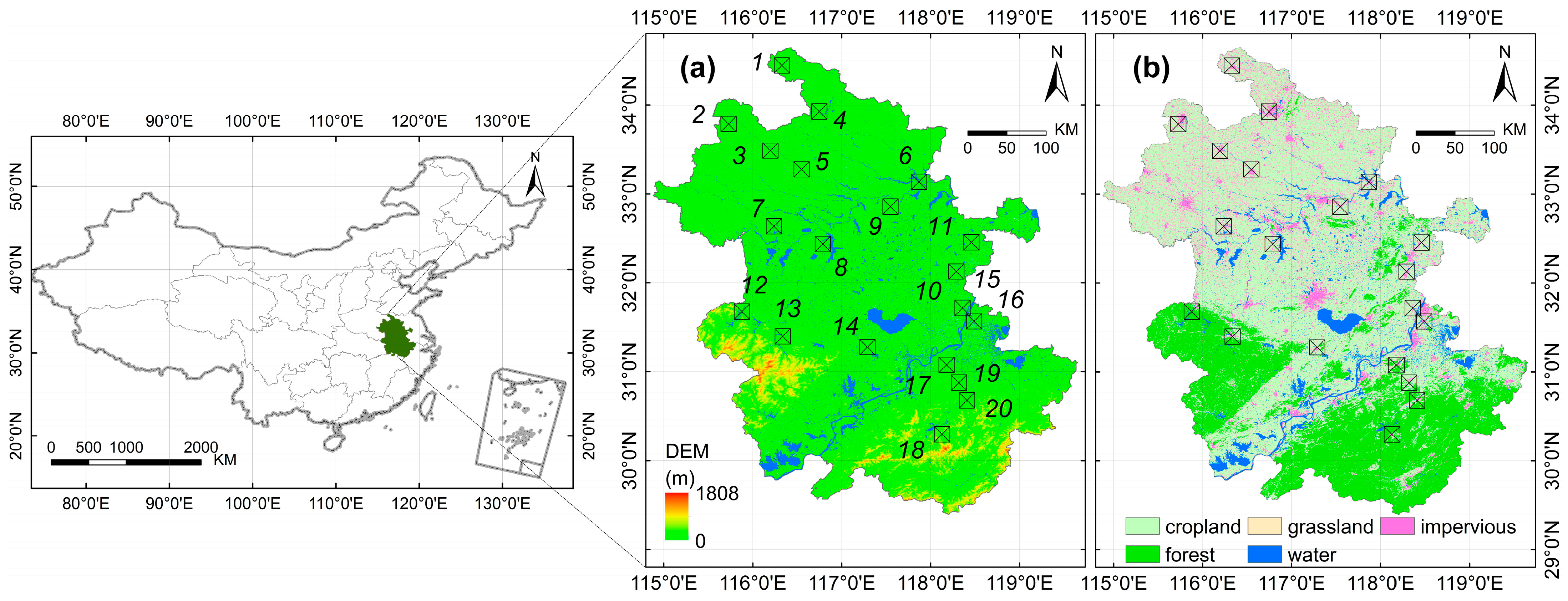
2.1. Study Area and In Situ Observations

Anhui Province, China (29°41′–34°38′N, 114°54′–119°37′E) is located in a humid to semi-humid transitional zone, known as a big agricultural province. The northern part of Anhui Province belongs to a semi-humid monsoon climate, and the southern part belongs to a subtropical humid monsoon climate. The annual mean temperature ranges from 14–16 °C, and the annual precipitation ranges from 800–1600 mm across the whole province [34]. Cropland is the main land-use land cover (LULC) type in the northern and central flat areas (Figure 1), where irrigation systems are essential to maintain agricultural production [35]. The northern part has no large lakes or rivers, whereas the central part is characterized by highly developed water systems, including the Yangtze River, the Huai River and the Chaohu Lake. The southern and southwestern areas are covered by hilly terrains with dense forests (Figure 1). A total of 20 meteorological stations (Table 1) recorded hourly SM data at a 10-cm depth beneath the soil surface in 2017–2020. The data were collected from the Anhui Meteorological Service Center and were checked for breaks and non-responsive values, following the method in [36]. The temporal consistencies of SM observations were checked by reference to multiple SM products (described below) to find any changes in sensor sensitivities (dynamic ranges) or obvious inconsistencies in SM trends. Finally, the mean SM values and SM dynamics (1σ) are shown in Table 1. The 0.05° × 0.05° monthly Terra Moderate-resolution Imaging Spectroradiometer (MODIS) normalized difference vegetation index (NDVI) data in 2017–2020 were extracted and averaged to show the mean vegetation conditions at each station.

2.2. Soil Moisture Products and Data Preprocessing

Multiple radiometer-based products were compared in this study. The Advanced Microwave Scanning Radiometer 2 (AMSR2) products are based on the Land Parameter Retrieval Model (LPRM), JAXA algorithm, Normalized Polarization Difference (NPD) algorithm and Single Channel Algorithm (SCA). LPRM simultaneously retrieves surface temperature, SM and VOD, producing three datasets at 10.7 GHz (X band), 6.9 GHz (C1 band) and 7.3 GHz (C2 band) [38]. JAXA retrieves SM and VOD based on a lookup table approach [39]. NPD uses the polarization difference and a combined vegetation/roughness factor, and SCA uses Advanced Very High Resolution Radiometer (AVHRR) NDVI climatology for vegetation correction [40]. Unlike LPRM, other algorithms only generate X-band SM products to mitigate radio frequency interference (RFI) effects. These products differ substantially from each other [41], which motivates new retrieval and merging algorithms [42,43]. For all AMSR2 products, SM values within 0–0.6 cm3·cm−3 were kept for validation.
Soil Moisture and Ocean Salinity (SMOS) products include SMOS-L3 V300 [44] and SMOS-IC V106 [45], derived from multi-angular TB observations by iterating the L-band Microwave Emission of the Biosphere forward model. Soil Moisture Active Passive (SMAP) products are generated based on three algorithms: SCA-H (H-pol), SCA-V (V-pol) and dual channel algorithm (DCA) [19]. The recent SMAP Version 8 SM products were validated in this study, with DCA as the baseline algorithm. Two versions of flagging strategies were applied for SMOS and SMAP. The rigorous one was the same as that in [46], which is commonly used in validation studies. Specifically, for SMOS-L3, data with a surface temperature < 273 K, quality index (Soil_Moisture_Dqx) > 0.06 or RFI probability (RFI_Prob) > 0.1 were excluded. SMOS-IC SM data with a surface temperature > 273 K and a quality flag = 0 (“data OK”) were retained. For SMAP products, data with retrieval quality index = 0 or 8 were retained. The relaxed one is the same to that for AMSR2, reserving all SM values within 0–0.6 cm3·cm−3. Both data in the a.m. and p.m. orbits were considered for radiometer-based products (Table 2).
Active-based products were also validated in this study. The National Aeronautics and Space Administration (NASA) Cyclone Global Navigation Satellite System (CYGNSS) product is generated by reference to The SMAP SCA-V, having the advantages of wide spatial and temporal coverage [47]. A 25-km MetOp-B Advanced Scatterometer (ASCAT) product was generated based on a change detection method [48]. SM values were retained only if wetland flag < 15%, topography flag < 20%, frozen soil probability < 10%, snow cover probability <10% and SM retrieval error < 10% [26]. The European Space Agency (ESA) Climate Change Initiative (CCI) V06.1 Active, Passive and Combined products were used in this study. The active and passive products are generated by fusing multiple satellite retrievals from scatterometers and radiometers, respectively, and the active and passive combined product is further rescaled to the Global Land Data Assimilation System (GLDAS) Noah SM climatology [49,50]. Data with snow cover, a surface temperature < 273 K, dense vegetation or failed retrievals were discarded. For ASCAT and ESA CCI Active, the degree of saturation was transformed into volumetric water content using the ESA CCI auxiliary porosity data. The nearest CCI porosity data were used to calculate the ASCAT SM.
Five modeling-based products were validated in this study. Forced by a number of analysis- and observation-based products [51], the GLDAS Noah land surface model can provide SM products in the 0–10 cm soil layer, which currently serves as the reference for rescaling ESA CCI SM. The Modern-Era Retrospective Analysis for Research and Applications Version 2 (MERRA2) is the latest atmospheric reanalysis of the modern satellite era produced by NASA’s Global Modeling and Assimilation Office (GMAO) [52], providing coarse-scale SM products in the 0–5 cm soil layer. ERA5 benefits from a decade of developments in model physics and data assimilation, providing enhanced modeling results compared to its predecessor, ERA-Interim [53]. It has been demonstrated that the direct assimilation of microwave-based SM products (e.g., SMAP SM and, recently, CYGNSS SM) into LSM improves SM modeling skills [13,54,55]. ERA5-Land shares with ERA5 most of the parameterizations and enhances the description of the hydrological cycle, in particular the soil moisture and lake description [56]. SMAP L4 product is derived by assimilating SMAP TB observations into the NASA Catchment Land Surface Model [57,58]. The basic properties of the modeling products are shown in Table 2. Note that only the products with the timestamp closest to UTC 0:00 were collected. For each product, SM data in the topmost layer were evaluated, and the data were discarded if the soil temperature was less than 273 K.

2.3. In Situ and Triple Collocation-Based Validations

A direct comparison of SM products with in situ observations is straightforward. For each station, quality-assured in situ SM observations and gridded SM products were spatially and temporally matched. The correlation coefficient (R), bias, ubRMSE and root mean square error (RMSE) values were calculated for each product. Taylor diagrams were used to compare R, RMSE and standard deviation (SD, square root of variance) values among these products. Based on the statistical analyses, the performance of each product was generalized. SD is a measure of the SM dynamic range. Low SD values mean low information content and exceptionally high SD values mean noisy retrievals. Correlation measures the overall consistency of SM products and observations. RMSE and ubRMSE measure the overall and bias-corrected SM differences, respectively. These metrics have been widely used in validation studies and are defined as follows:
R = i = 1 N ( x i x ¯ ) ( y i y ¯ ) i = 1 N ( x i x ¯ ) 2 i = 1 N ( y i y ¯ ) 2
Bias = i = 1 N ( y i x i )
RMSE = i = 1 N ( y i x i ) 2 N
ubRMSE   =   RMSE 2 Bias 2
SD = i = 1 N ( x i x ¯ ) 2 N
where x is in situ SM observation, y is gridded SM product, the overbar denotes the mean value, and N denotes the number of data pairs.
The TCA was performed by considering the scale difference of multiple SM products. TC-based correlation coefficient (TC_R) and RMSE (TC_RMSE) values can be calculated based on three error-independent datasets, usually composed of a passive-based, an active-based and a modeling-based dataset [20,28]. TC_R and TC_RMSE show the correlation and overall difference between each triplet and the ‘true’ SM time series. For TCA, SM data in the a.m. and p.m. orbits were averaged to increase the sample size. The time series of SM anomaly was calculated based on a 31-day moving window, similar to [19], and the minimum length of the time series was 100. A critical hypothesis of TCA is the zero error cross-correlation (ECC) between SM triplets, which is usually violated even for active- and passive-based products. The consequence is that the evaluation results differ among triplets. Here, we calculated TC_R and TC_RMSE values for any possible triplet to find the lower and upper boundaries of the two metrics values. We are aware that optimistic statistics can be obtained by including ECC-dependent products in TCA (e.g., SMAP and CYGNSS or ERA5 and ASCAT in a triplet), and the statistics might vary greatly among triplets [32]. Therefore, the median TC_R and TC_RMSE values were compared. Although the median values might still be biased, they can be used for a fair comparison among sites and products. All data processing was accomplished based on the MATLAB R2015a platform. The mathematical form of TC_R and TC_RMSE is defined as follows:
TC _ R X = σ X Y σ X Z σ X X σ Y Z
TC _ RMSE X = σ X X σ X Y σ X Z σ Y Z
where X, Y and Z denote independent time series of SM anomaly (N > 100), σ denotes variance (for one dataset) or covariance (for two datasets).

2.4. Evaluating the Capabilities of Precipitation and Irrigation Detection

Precipitation and irrigation are the dominant natural and human factors of SM dynamics. The ability of multiple SM products to respond to precipitation signals was first evaluated. To this end, the 0.1° × 0.1° daily integrated multi-satellite retrievals for Global Precipitation Measurement (IMERG) precipitation product [59] were collected. For each station, the daily precipitation amount (cumulative P in UTC 0:00–UTC 0:00, approximately local time 8 a.m.–8 a.m.) was calculated and correlated with daily SM change (ΔSM) in 24 h. To match precipitation and SM products, the in situ observations at 8 a.m., the SMOS/SMAP/ASCAT a.m. products (6 a.m., 9:30 a.m.), and the daily averaged AMSR2 products were used. The other products were composed to 8 a.m. or generated at 8: 00–9:30 a.m. (Table 2), with minimal time differences from the precipitation product. Correlation coefficients were calculated between daily P and ΔSM for in situ SM observations and SM products in order to evaluate the diverse responses of SM dynamics to precipitation. Because no in situ precipitation data were available, only IMERG precipitation data were used in this study.
The ability of multiple SM products to capture irrigation signals was evaluated. To this end, the monthly irrigation water use (IWU) product [33] was collected. Recently, Zhang et al. [33] considered multiple irrigation-related processes in the framework of hydrological balance and integrated multiple satellite observations to obtain ensemble IWU estimates from 2011–2018. To match the IWU product, multiple SM products were calculated to monthly averages. Because meteorological stations are not distributed in cropland areas, the observations only reflect precipitation signals. The difference between gridded products and in situ observations should reflect, if any, irrigation signals. Based on this hypothesis, the monthly SM difference (gridded minus in situ) was correlated with the monthly IWU. The stronger the correlationship, the better the capability of SM products to capture irrigation signals. Although representativeness errors might have an impact, results concluded from the 20 stations provide insight into the selection of irrigation-sensitive SM products.

3. Results

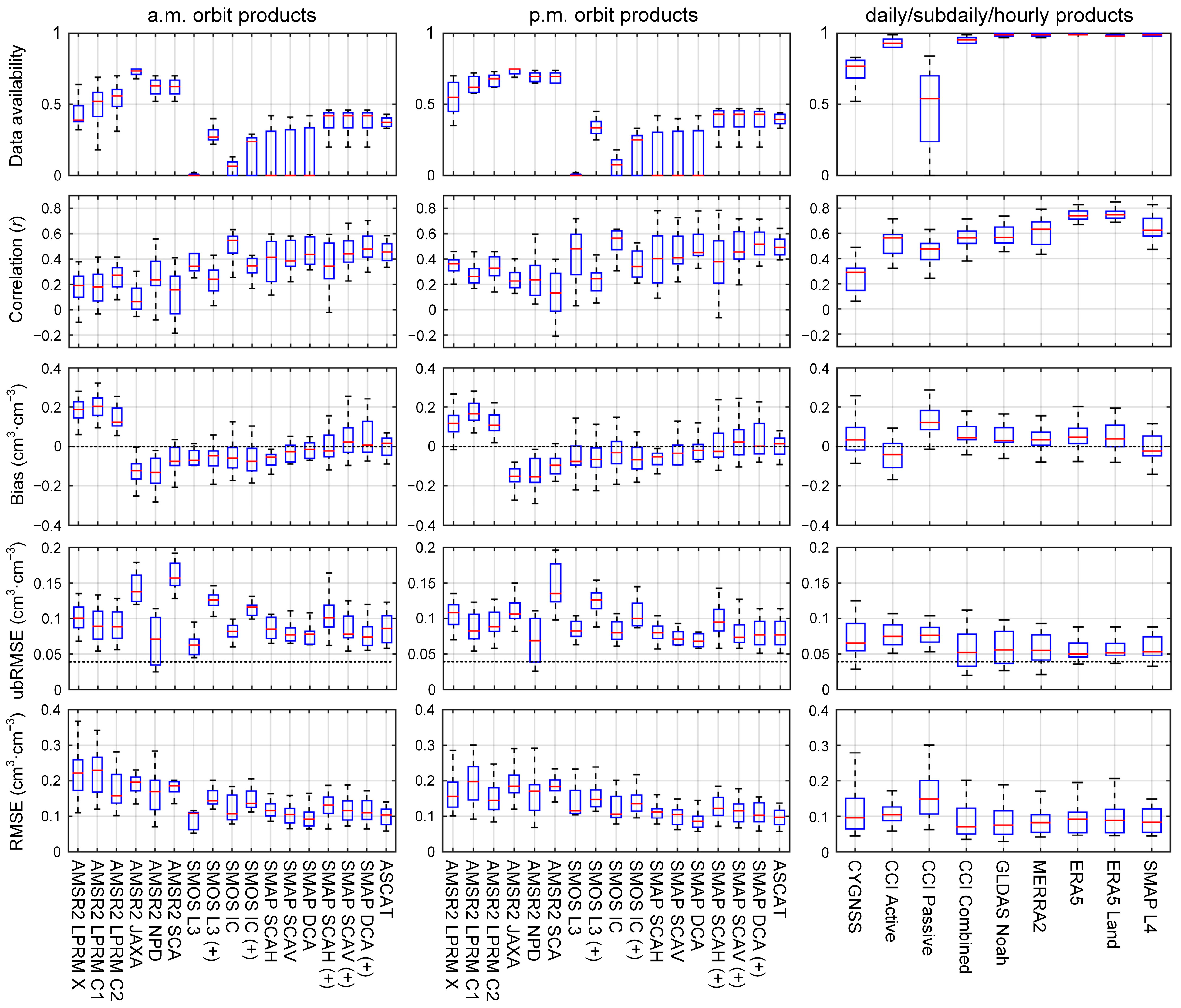
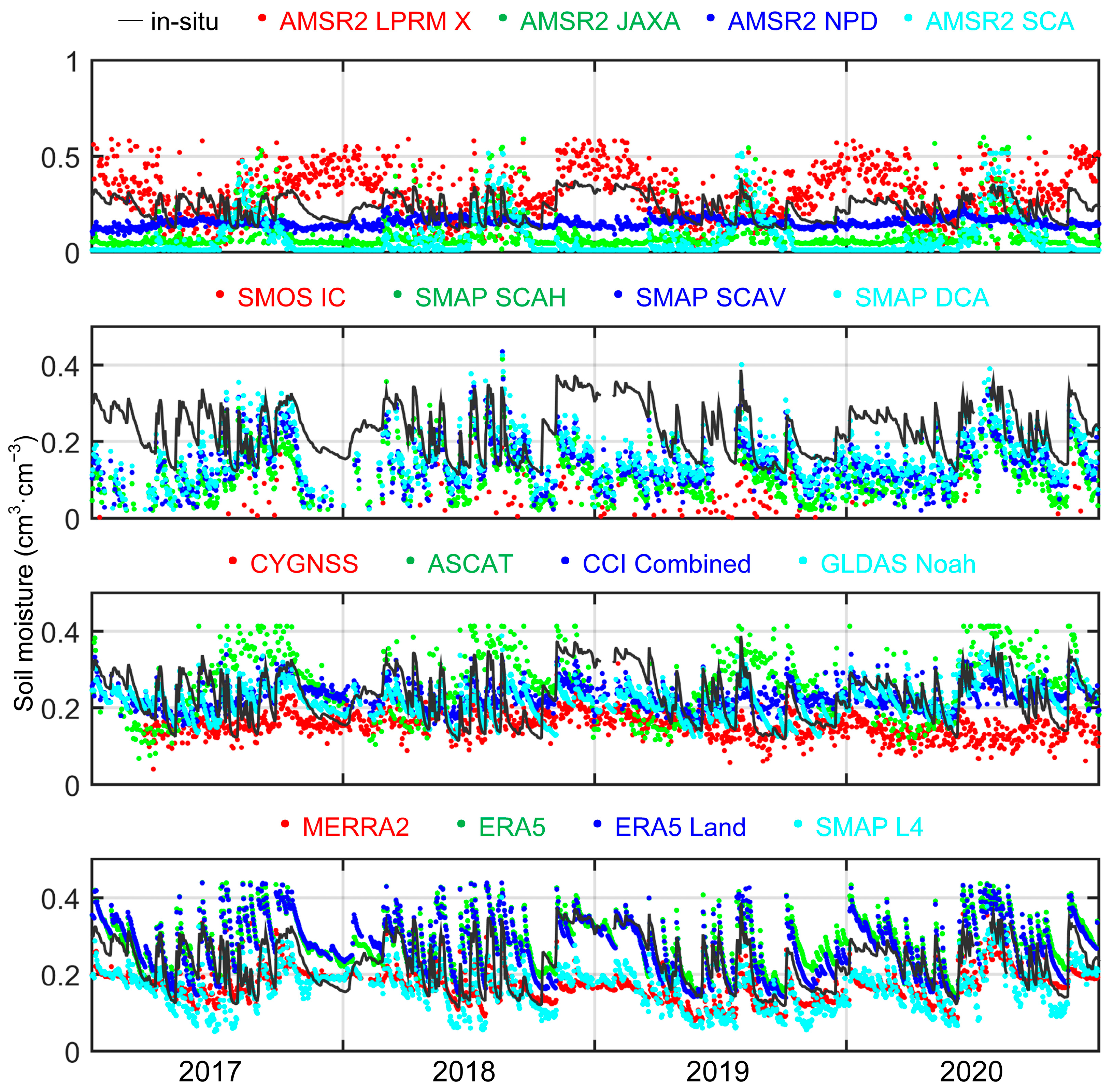
3.1. Overall Performance of SM Products

Figure 2 shows the statistical values for the validation of SM products at the 20 stations. Each boxplot shows the maximum, 75% quartile statistics, median, 25% quartile statistics and the minimum of the metrics, including data availability, correlation coefficient, bias, ubRMSE and RMSE for the 20 stations. Data availability means the proportion of quality assured SM data in the study period of 2017–2020. Generally, models provide more SM data than remote sensing, demonstrating the advantages of wide spatial and temporal coverage. Only minor data of frozen soils (<5%) are discarded. ESA CCI Combined and Active have provided more than 90% data in recent years, followed by CYGNSS. All AMSR2 products provide 50–80% data, most for JAXA and least for LPRM X. ASCAT provides about 40% data, whereas SMOS and SMAP provide much less data (<10%) due to a strict operational flagging strategy. A relaxed strategy (0–0.60 cm3·cm−3) can largely increase data volume for L-band products (Figure 2). ESA CCI Passive has a wide range of data availability, as it integrates AMSR2, SMOS and SMAP data.
Modeling-based products generally outperform remote sensing-based products. ERA5 and ERA5 Land can better capture SM dynamics (R ≈ 0.8) and have lower and more stable ubRMSE values than other products. Despite large differences in spatial resolution, MERRA2 and SMAP L4 provide almost unbiased SM data and have minimal differences from observations. For remote sensing, the L-band outcompetes C-/X-band for SM retrieval. The former has consistent data quality in the a.m. and p.m. orbits. In the L-band, SMAP products have lower uncertainties, although SMOS-IC outperforms in terms of correlation. Regarding ubRMSE and RMSE, SMAP DCA performs the best, followed by SMAP SCA-V, SCA-H and SMOS-IC (SMOS-L3 not included due to low data volume). SMAP DCA is almost unbiased, similar to ASCAT. A relaxed flagging strategy increases the L-band data volume, yet the data quality is not necessarily largely decreased (especially for R). All AMSR2 products are not well-correlated with the observations (R < 0.4). NPD performs the best, followed by LPRM C2, and JAXA and SCA have the largest ubRMSE values. Positive biases are observed for LPRM products and negative for other AMSR2 products. The differences in bias can be as large as 0.03 cm3·cm−3.
ESA CCI and ASCAT are better than other remotely sensed products, considering both data availability and accuracy. ESA CCI Combined performs the best, followed by ESA CCI Active and Passive. ASCAT is the optimal single-satellite-based product, outperforming SMAP and SMOS in data availability and AMSR2 in overall accuracy. Integration of ASCAT and other radar data makes ESA CCI Combined the best remotely sensed product. ESA CCI Combined is positively biased, similar to GLDAS Noah, as the former is rescaled to the latter. Larger positive and negative biases were observed for ESA CCI Active and Passive, respectively. CYGNSS significantly extends the spatial coverage of SMAP data while at the expense of reduced data quality, which is even lower than that of poorly flagged SMAP data.

3.2. Specific Behaviors of SM Products

Figure 3 shows Taylor diagrams of all SM products for two cropland stations (Figure 3a,b) and one forest land station (Figure 3c). All modeling-based products report large SM dynamics in cropland and low SM dynamics in forest land. ERA5 and ERA5 Land have wider SM dynamic ranges and consistently stronger correlations with observations than other products. Modeling-based products are closer to in situ observations than remote sensing-based products, including ESA CCI Combined, which is rescaled to GLDAS Noah. AMSR2 products differ greatly among algorithms. The JAXA and SCA products are close to each other.
Figure 4 shows that most products can capture short-term SM dynamics well, except for AMSR2 and CYGNSS. AMSR2 LPRM’s perform similarly and have wide SM dynamic ranges, with unexpectedly large values in the winter season. Only LPRM X-band retrievals are shown in Figure 4 for comparison with other AMSR2 X-band retrievals. AMSR2 JAXA and SCA have abnormally high values in the summer season and consistently low values (~0.01 cm3·cm−3) in other seasons. AMSR2 NPD has a very narrow SM dynamic range. CYGNSS also has a narrow SM dynamic range with large short-term noises. SMAP products are in better agreement with in situ observations than SMOS-IC and SMOS-L3 (not shown due to the low data volume). All ESA CCI products reproduce well in situ observed SM dynamics. For ESA CCI Combined, data fusion and rescaling to GLDAS Noah SM reduces dry biases in ESA CCI Active and wet biases in ESA CCI Passive. ASCAT performs similarly to ESA CCI Active, but the retrievals are almost unbiased.
Forced by meteorological datasets, all modeling-based products can well reproduce the temporal pattern of SM variabilities. It is interesting to observe that the 0–10 cm ERA5 and ERA5 Land products fit better with in situ observations for dry soils, and the 0–5 cm MERRA2 and SMAP L4 products fit better for wet soils (Figure 4). The depth of the top soil layer and the quality of the forcing datasets might account for the differences. A detailed comparison of in situ observations is shown in Figure 5. Considering data availability and overall accuracy, only six major products are presented here. Regression slope values can manifest the dynamic range of SM values. ERA5 has the largest SM dynamic range, followed by SMAP L4, MERRA2, ESA CCI Combined, GLDAS Noah and CYGNSS.

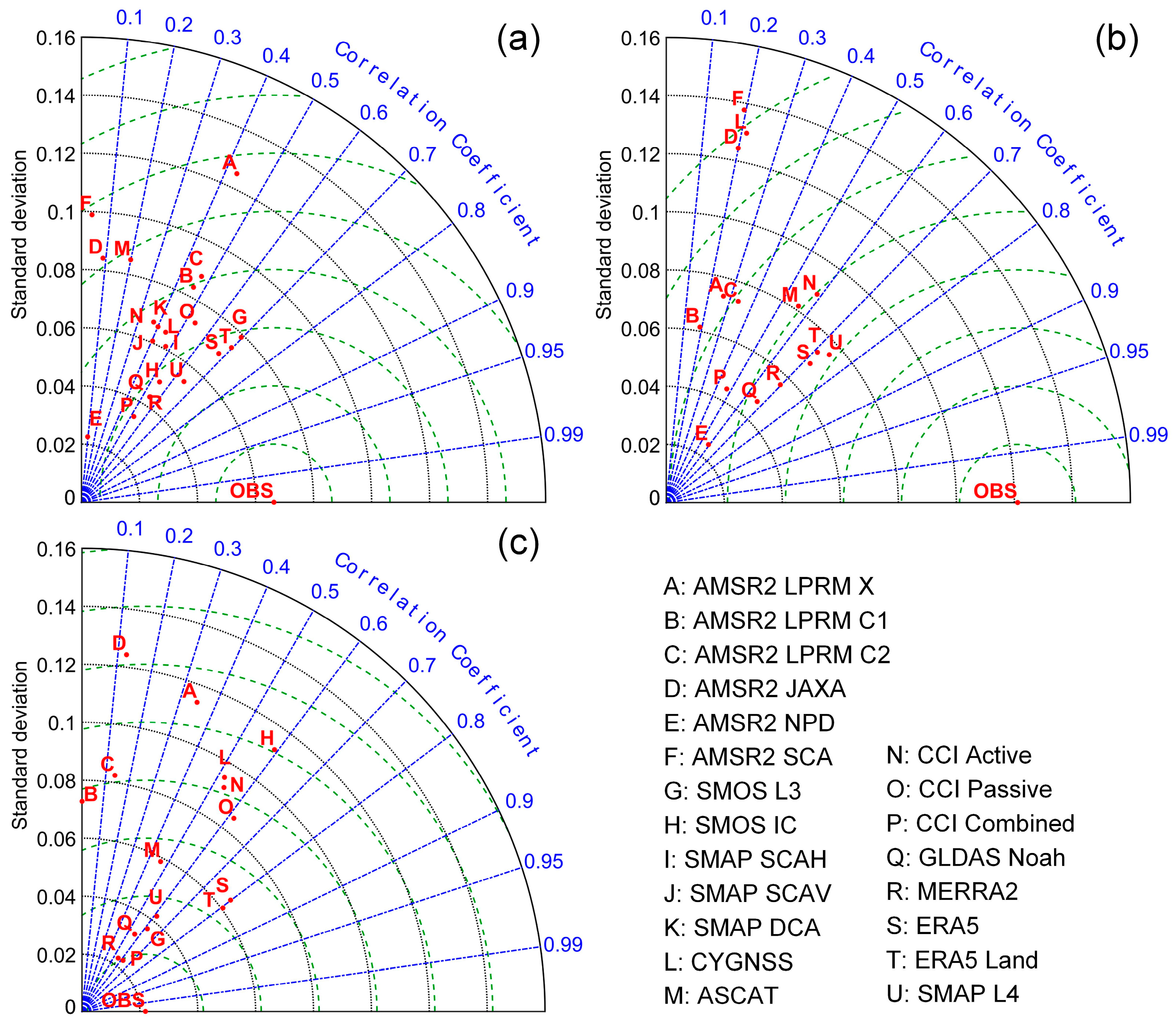
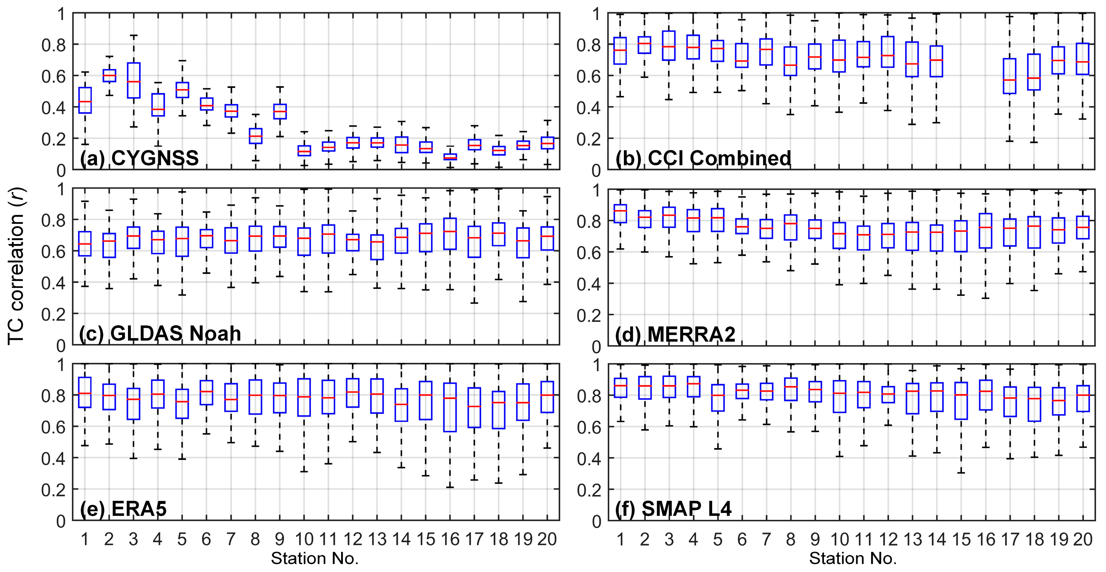
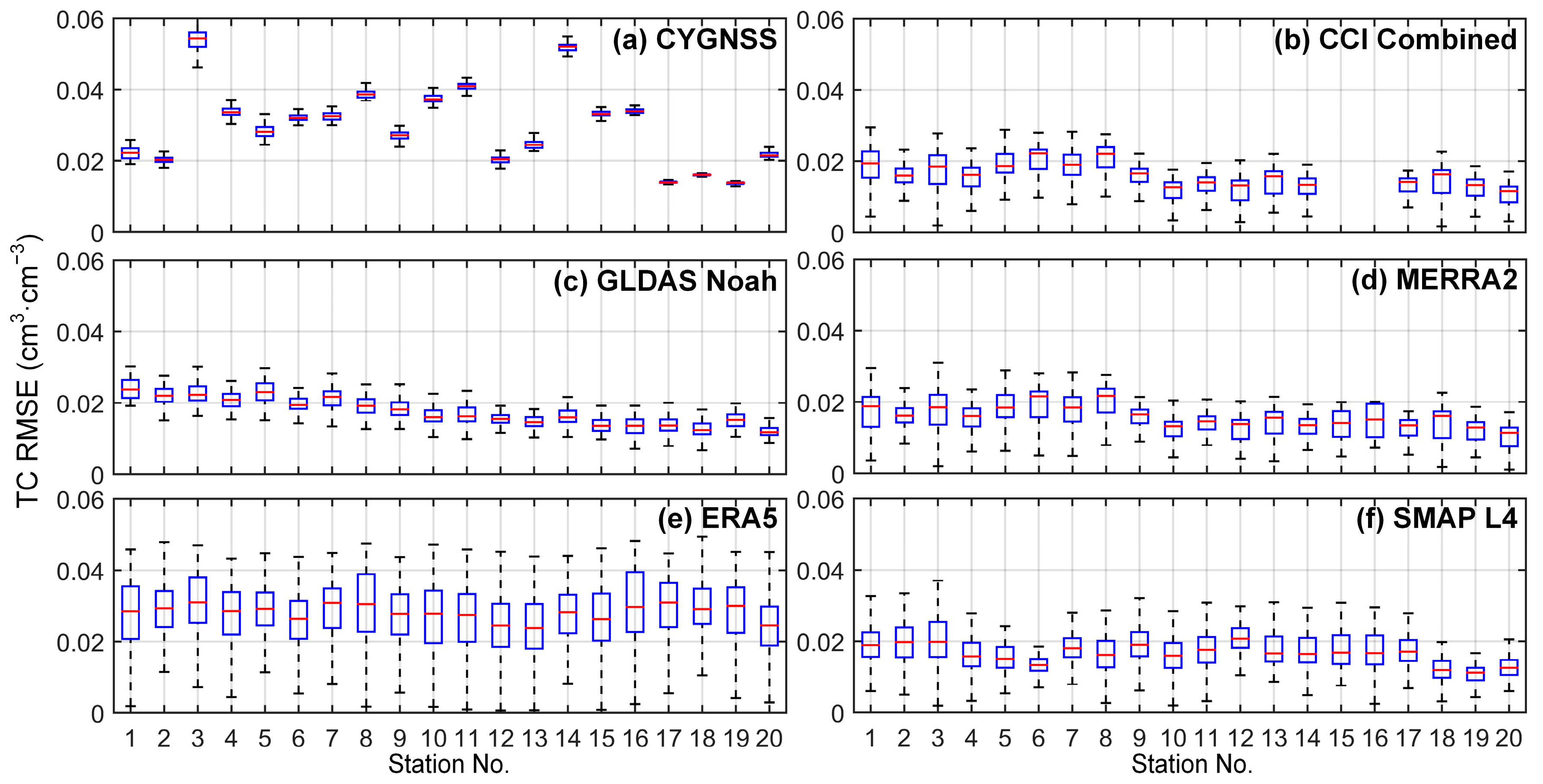
3.3. TC-Based Comparison of SM Products

TC-based correlations confirm the advantages of models over remote sensing, especially in the central water-contaminated and southern hilly areas. CYGNSS has a moderate correlation in the northern plain, where SMAP products also perform better. SMAP cannot provide enough quality-assured data for calibrating CYGNSS in the rest of study area, leading to decreased CYGNSS data quality (R < 0.2, Figure 6a). ESA CCI Combined has also decreased data quality in these areas (Figure 6b), where satellite-based SM retrievals generally have large uncertainties. Especially in forest areas, low SM dynamics and high retrieval uncertainties contribute to low correlations. Model performances are less dependent on land cover. SMAP L4 and ERA5 perform better in the northern plain, and the performance decreases marginally in the rest of the study area. Compared to GLDAS Noah and MERRA2, the assimilation-based ERA5 and SMAP L4 performed slightly better in the central and southern areas. Together with ESA CCI Combined, all modeling-based products have ubRMSE values that are better than 0.04 cm3·cm−3, except for ERA5 (Figure 7). Although ERA5 shows a median RMSE value better than 0.04 cm3·cm−3, the RMSE values are generally larger than other modeling-based products and exceed 0.04 cm3·cm−3 for some triplets. It seems that TC-based RMSE depends on the dynamic range of SM products. A wide SM dynamic range (e.g., for ERA5) might also amplify random errors, and a narrow SM dynamic range produces low σXX values in Equation (7) and thus low RMSE values.

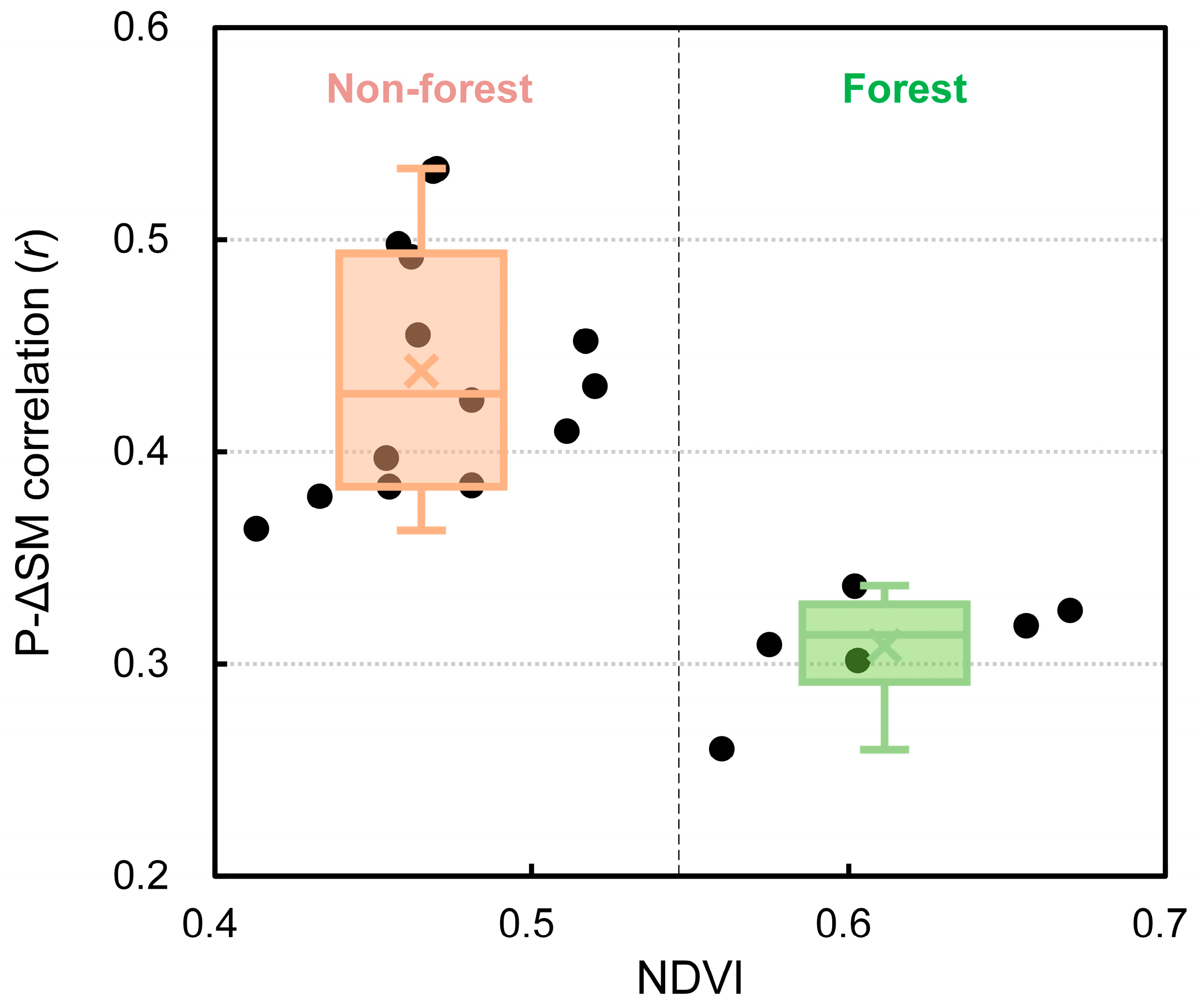
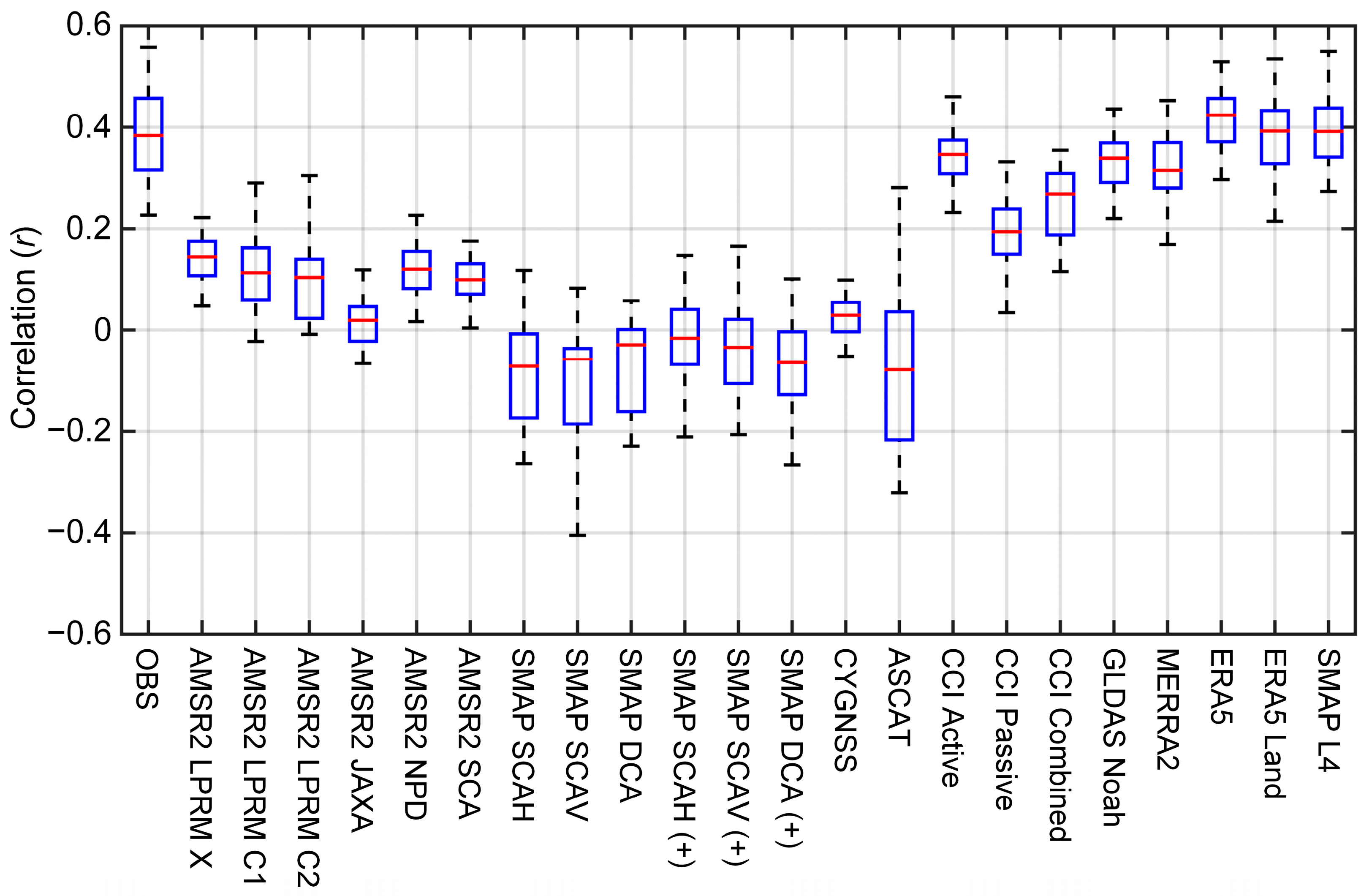
3.4. Diverse SM Responses to Precipitation Events

In situ observations show stronger SM responses to precipitation in cropland (R = 0.4) than in forest land (R = 0.3) (Figure 8). The responses of SM products to precipitation are shown in Figure 9. Among other AMSR2 products, LPRM X can best reproduce the correlation (R > 0.15) and JAXA the worst (almost uncorrelated). No SMOS results are available because of the low data volume. SMAP products also show weak correlations, and a relaxed flagging strategy does not improve performance. CYGNSS produces slightly better correlations than SMAP, attributable to higher data availability. A single satellite-based ASCAT product cannot reflect SM dynamics due to precipitation events. Integrating both MetOp-A and MetOp-B ASCAT data, ESA CCI Active shows much improved correlations (R > 0.3). ESA CCI Passive performs better than any individual radiometer-based product in response to precipitation, and the responsiveness of ESA CCI Combined is further enhanced by blending the Active product. All modeling-based products show close responsiveness to in situ observations. ERA5 performs the best, followed by SMAP L4, ERA5 Land, GLDAS Noah and MERRA2. However, with a finer spatial resolution, ERA5 Land does not perform as well as ERA5. These modeling-based products are forced by diverse precipitation datasets. However, the good data quality shared by precipitation datasets in this data-rich area is likely the major reason for the strong SM responses to IMERG-based precipitation.

3.5. Diverse SM Responses to Irrigation Events

The ability to capture irrigation signals differs among products and algorithms (Figure 10). As expected, modeling-based products can barely capture irrigation signals (R < 0.3), even though satellite data are assimilated (e.g., for ERA5 and SMAP L4). The radar-based ASCAT product is almost insensitive to irrigation signals, and ESA CCI Active further decreases sensitivity. Despite the low data volume, SMAP products are the most sensitive to irrigation signals. SMAP SCA-H and SCA-V have stronger sensitivities (R > 0.5) than SMAP DCA, although the latter shows better overall accuracy. It is noteworthy that the relaxed flagging strategy does not deprive SMAP of its ability to capture irrigation signals. The good performance even transfers to CYGNSS. SMOS products are less effective than SMAP products because of their lower data volume and overall accuracy. Due to contrasting SM values in cropping (high SM) and non-cropping (low SM) seasons (Figure 4), it is not surprising to see AMSR2 JAXA and SCA are strongly correlated (R > 0.5) with irrigation water use. It seems that single-channel algorithms are more competent than LPRM algorithms for detecting irrigation signals. With an LPRM algorithm, all three AMSR2 LPRM products and the ESA CCI Passive product have negative correlations (R < −0.3) with irrigation water use.

4. Discussion

4.1. Practices for Optimal Product and Algorithm Selection

No SM products perform consistently better than others. Modeling-based products have the advantages of continuous spatial and temporal coverage, strong correlations with in situ observations, and timely responses to rainfall events. Despite less accurate forcing data over poorly gauged areas, models still perform better and more consistently across different landscapes than remote sensing. The latter does not perform well or even fails to produce meaningful retrievals in the central and southern parts of Anhui province. The main difficulties include the separation of water emissions and the effects of complex terrains and/or dense vegetation. This is evidenced by the extremely low data volume of operational SMOS and SMAP products. As a result, data assimilation (e.g., SMAP L4) can marginally improve SM modeling in these areas. Recently, several studies have demonstrated the limited contribution of data assimilation to SM and carbon fluxes modeling under different circumstances [9,60]. This might also explain the large uncertainties of the CYGNSS product, which uses the SMAP product as a calibration reference. The increased coverage of the CYGNSS product is at the expense of decreased accuracy. Although AMSR2 products are not acceptable in terms of absolute accuracy, JAXA and SCA detect plausible irrigation signals. It is more likely a coincidence arising from high SM biases in cropping seasons and low biases in non-cropping seasons. If we focus on the detection of irrigation events, SMAP products are an optimal choice, especially SCA products.
High-resolution SM products are necessary for regional-scale drought monitoring [61,62], especially in intensive agricultural regions. ERA5 Land performs better than or at least comparably to ERA5 in terms of multiple metrics (Figure 2), providing a finer-resolution (~9 km) alternative for drought monitoring. This study corroborates the current use of ERA-5 Land SM for drought monitoring in Anhui province. Remote sensing offers an objective description of land surfaces. However, the products do not correlate as well with in situ observations or respond as well to rainfall events on a daily scale. Short-term random noises might be the major reason. As a result, temporal aggregation can improve the comparability of remotely sensed and modeling-based products. For example, Liu et al. [63] observed a slightly better performance of ESA CCI over GLDAS Noah for global drought monitoring on a monthly scale. Moreover, an ensemble of results from multiple datasets is recommended.

4.2. Implications for Improving the Retrieval Algorithm

AMSR-E and AMSR2 provide over 20 years of multifrequency global observations. Several retrieval algorithms have been developed, among which LPRM C2 and NPD stand out in this study. More stringent flagging strategies might improve the evaluation metric values, especially considering the RFI effects. Poor flagging partly contributes to a high percentage of data availability and, in the meantime, causes low data quality. This applies equally to other AMSR2 products. AMSR2 SCA has high values in wet seasons and low values in dry seasons. Soil and vegetation parameters can be refined for better retrieval as SCA proves to be successful and serves previously as a baseline algorithm for SMAP. More importantly, it is necessary to rethink the appropriate parameterization, as multiple retrieval algorithms have diverse SM biases.
SMAP SCAs have proven superior abilities in capturing irrigation signals. The use of real-time instead of climatological vegetation data might further improve SM retrievals and the detectability of irrigation signals because cropland phenology experiences substantial inter-annual variabilities [64,65]. Water correction is critical to SM retrieval in regions with a dense network of rivers and lakes. This is probably the main reason for the decreased SM accuracy in the central Anhui province. The distribution of complex terrains and dense forests explains the low SM accuracy in the south. Both effects apply equally to other remotely sensed products but are not decisive for modeling-based products. Recent studies have shown SM sensitivities of L-band radiometry under temperate forest canopies and deeper than a few centimeters [66,67]. This might improve SM retrieval under dense vegetation cover. Biases in effective soil surface temperature data also play a role in SM retrieval [46,68,69], especially under dense vegetation cover that masks out a large portion of soil emissions.
The ESA and NASA effects on GNSS-R for SM retrieval have been well elaborated upon by Pierdicca et al. [70]. This technique is currently far from mature for SM retrieval, although more advanced algorithms have been recently developed, e.g., change detection in [71], machine learning in [72,73] and semiempirical method in [74]. The currently operational CYGNSS SM product is generated using a linear relationship calibrated between reflectivity and SMAP SM. The residual nonlinearities and uneven distribution of calibration samples explain the reduced SM dynamic range, i.e., underestimating high SM values and overestimating low SM values [70]. The same issue is also encountered in remote sensing of soil salinity based on linear regression [75]. Moreover, CYGNSS retrievals are also affected by low-quality SMAP data and noisy observations over mountainous regions, making SM time series noisier than SMAP. To meet both ends, nonlinear and physically based methods are needed for further improvement. For nonlinear methods, such as machine learning [72,73], high-quality satellite retrievals are still required.
LPRM products (AMSR2 and ESA CCI Passive) show strong negative correlations between irrigation water use and SM bias. The underestimation of high SM values and/or overestimation of low SM values might be responsible. Although spatial scales differ between product grids and site observations, SMAP products still show strong positive correlations. At the least, LPRM products are biased from SMAP products. This result underscores the importance of comparing multiple SM climatology [76] and further investigation into the LPRM algorithm.

4.3. Recommendations for Validation of Soil Moisture Products

Validation practices for satellite soil moisture products have been well documented by Gruber et al. [11]. The representativeness of in situ sites is emphasized in this study. Meteorological stations record long-term soil moisture observations, which are invaluable for validation purposes. However, these stations are distributed for ease of management, generally far away from agricultural land. The observations only naturally reflect soil drying and wetting processes and are unaffected by irrigation events. This might be one of the reasons for better model performance than remote sensing. Based on MODIS products, we observed a recent (2000–2021) NDVI decreasing trend at the 20 meteorological stations. The intensive urbanization processes in China might lower the representativeness of in situ observations. The measurement depth of in situ data is also a critical factor affecting the validation results. The 10-cm measurement depth is closer to that of modeling-based products, e.g., 0–5 cm, 0–7 cm and 0–10 cm, which produces better validation metrics values. Remotely sensed products have a shallower penetration depth of 0–2 cm at the X- and C-bands and 0–5 cm at the L-band. The inconsistencies in soil depth underscore the difficulties in SM product evaluation, especially for biases.
The other recommendation is on the validation method. TCA has several assumptions and the results might differ among triplets. The basic assumption is a linear relationship between SM datasets and the unknown true SM time series plus zero-mean random noise. The core assumption is zero error cross-correlation between SM datasets, which is not held even for passive- and active-based retrievals. Although it is feasible to examine this assumption by introducing a fourth dataset [24], using multiple triplets is more practical. For example, Zheng et al. [27] used multiple triplets and a bootstrapping technique to enhance the TCA results. Similarly, in this study, the method can depict the upper and lower boundaries of TC-based metric values. It becomes more useful with a growing number of products from observations, models and remote sensing. The median correlation and RMSE values are more robust, reducing the risk of over-optimistic evaluation results.

5. Conclusions

This study compared multiple remotely sensed, modeling- and assimilation-based SM products against in situ observations in a humid to semi-humid transitional region with diverse landscapes. Models generally outperform remote sensing in hilly and densely vegetated areas and areas with developed water systems. Remote sensing has difficulties in these areas, as evidenced by the extremely low data volume of operational SMOS and SMAP products. The limited and noisy SMAP reference data are mainly responsible for the low accuracy and narrow dynamic range of the CYGNSS product. For the same reason, data assimilation can marginally improve SM modeling. AMSR2 products have diverse but generally low performances depending on retrieval algorithms, which is better for LPRM C2 and NPD in terms of overall accuracy. ASCAT is the optimal single-satellite product, having both acceptable accuracy and spatial coverage. Models can better reproduce the responses of SM to precipitation events than remote sensing, while by nature they cannot reflect irrigation events. SMAP SCA-H and SCA-V are among the best products for detecting irrigation signals. The plausible irrigation signals revealed by AMSR2 SCA and JAXA are likely caused by retrieval errors. All LPRM products failed to identify irrigation events, probably due to an overestimation of low SM values and/or an underestimation of high SM values. The evaluation results provide guidance to select optimal products, improve retrieval algorithms and recommend common practices for SM validation.

Author Contributions

Conceptualization, X.F. and Y.L. (Yanyu Lu); methodology, X.F. and Y.L. (Yongwei Liu); formal analysis, X.F., Y.L. (Yongwei Liu) and S.X.; resources, T.L.; data curation, X.F.; writing—original draft preparation, X.F.; writing—review and editing, X.F., Y.L. (Yanyu Lu) and T.L.; funding acquisition, X.F., X.Z. and Y.L. (Yanyu Lu). All authors have read and agreed to the published version of the manuscript.

Funding

This research was funded by the National Natural Science Foundation of China, grant number 42171365 and 41971046, and the Key Research and Development Program of Anhui, grant number 2022m07020003.

Data Availability Statement

The AMSR2 LPRM SM product can be found here: https://disc.gsfc.nasa.gov/datasets?keywords=AMSR2; the AMSR2 JAXA SM product can be found here: ftp://ftp.gportal.jaxa.jp; the AMSR2 LANCE (NPD and SCA) SM product can be found here: https://n5eil01u.ecs.nsidc.org/DP1/AMSA/AU_Land.001/; the SMOS L3 and SMOS IC SM products can be found here: ftp://ftp.ifremer.fr; the SMAP L3 SM product can be found here: https://nsidc.org/data/SPL3SMP/versions/8; the CYGNSS SM product can be found here: https://data.cosmic.ucar.edu/gnss-r/soilMoisture/cygnss/level3/; the ASCAT SM product can be found here: https://navigator.eumetsat.int/product/EO:EUM:DAT:METOP:SOMO25; the ESA CCI SM product can be found here: https://esa-soilmoisture-cci.org/data; the GLDAS Noah SM product can be found here: https://ldas.gsfc.nasa.gov/gldas/; the MERRA2 SM product can be found here: https://disc.gsfc.nasa.gov/datasets?keywords=MERRA2; the ERA5 SM product can be found here: https://www.ecmwf.int/en/forecasts/datasets/reanalysis-datasets/era5; the ERA5 Land SM product can be found here: https://www.ecmwf.int/en/forecasts/dataset/ecmwf-reanalysis-v5-land; the SMAP L4 SM product can be found here: https://nsidc.org/data/SPL4SMGP/versions/6; the MODIS NDVI product can be found here: https://ladsweb.modaps.eosdis.nasa.gov/. The GPM IMERG precipitation product can be found here: https://disc.gsfc.nasa.gov/datasets/GPM_3IMERGDF_06/summary?keywords=%22IMERG%20final%22; the irrigation water use product is openly available in National Tibetan Plateau/Third Pole Environment Data Center (TPDC) at doi.org/10.11888/hydro.tpdc.271220; A registration is generally compulsory for data collection. In-situ soil moisture data are not publicly available due to data privacy policy.

Conflicts of Interest

The authors declare no conflict of interest.

References

  1. Seneviratne, S.I.; Corti, T.; Davin, E.L.; Hirschi, M.; Jaeger, E.B.; Lehner, I.; Orlowsky, B.; Teuling, A.J. Investigating soil moisture—Climate interactions in a changing climate: A review. Earth-Sci. Rev. 2010, 99, 125–161. [Google Scholar] [CrossRef]
  2. Brocca, L.; Ciabatta, L.; Massari, C.; Camici, S.; Tarpanelli, A. Soil Moisture for Hydrological Applications: Open Questions and New Opportunities. Water 2017, 9, 140. [Google Scholar] [CrossRef]
  3. Walker, J.P.; Willgoose, G.R.; Kalma, J.D. In situ measurement of soil moisture: A comparison of techniques. J. Hydrol. 2004, 293, 85–99. [Google Scholar] [CrossRef]
  4. Dorigo, W.; Himmelbauer, I.; Aberer, D.; Schremmer, L.; Petrakovic, I.; Zappa, L.; Preimesberger, W.; Xaver, A.; Annor, F.; Ardö, J.; et al. The International Soil Moisture Network: Serving Earth system science for over a decade. Hydrol. Earth Syst. Sci. 2021, 25, 5749–5804. [Google Scholar] [CrossRef]
  5. Mo, T.; Choudhury, B.J.; Schmugge, T.J.; Wang, J.R.; Jackson, T.J. A model for microwave emission from vegetation-covered fields. J. Geophys. Res. Earth Surf. 1982, 87, 11229–11237. [Google Scholar] [CrossRef]
  6. Wigneron, J.-P.; Jackson, T.; O’Neill, P.; De Lannoy, G.; de Rosnay, P.; Walker, J.; Ferrazzoli, P.; Mironov, V.; Bircher, S.; Grant, J.; et al. Modelling the passive microwave signature from land surfaces: A review of recent results and application to the L-band SMOS & SMAP soil moisture retrieval algorithms. Remote Sens. Environ. 2017, 192, 238–262. [Google Scholar] [CrossRef]
  7. Dorigo, W.A.; Scipal, K.; Parinussa, R.M.; Liu, Y.Y.; Wagner, W.; de Jeu, R.A.M.; Naeimi, V. Error characterisation of global active and passive microwave soil moisture datasets. Hydrol. Earth Syst. Sci. 2010, 14, 2605–2616. [Google Scholar] [CrossRef] [Green Version]
  8. Liu, Y.Y.; Dorigo, W.A.; Parinussa, R.M.; de Jeu, R.A.M.; Wagner, W.; McCabe, M.F.; Evans, J.P.; van Dijk, A.I.J.M. Trend-preserving blending of passive and active microwave soil moisture retrievals. Remote Sens. Environ. 2012, 123, 280–297. [Google Scholar] [CrossRef]
  9. Dong, J.; Crow, W.; Reichle, R.; Liu, Q.; Lei, F.; Cosh, M.H. A Global Assessment of Added Value in the SMAP Level 4 Soil Moisture Product Relative to Its Baseline Land Surface Model. Geophys. Res. Lett. 2019, 46, 6604–6613. [Google Scholar] [CrossRef]
  10. Khandan, R.; Wigneron, J.-P.; Bonafoni, S.; Pour Biazar, A.; Gholamnia, M. Assimilation of Satellite-Derived Soil Moisture and Brightness Temperature in Land Surface Models: A Review. Remote Sens. 2022, 14, 770. [Google Scholar] [CrossRef]
  11. Gruber, A.; De Lannoy, G.; Albergel, C.; Al-Yaari, A.; Brocca, L.; Calvet, J.-C.; Colliander, A.; Cosh, M.; Crow, W.; Dorigo, W.; et al. Validation practices for satellite soil moisture retrievals: What are (the) errors? Remote Sens. Environ. 2020, 244, 111806. [Google Scholar] [CrossRef]
  12. Schaefer, G.L.; Cosh, M.H.; Jackson, T.J. The USDA Natural Resources Conservation Service Soil Climate Analysis Network (SCAN). J. Atmos. Ocean. Technol. 2007, 24, 2073–2077. [Google Scholar] [CrossRef]
  13. Ling, X.; Huang, Y.; Guo, W.; Wang, Y.; Chen, C.; Qiu, B.; Ge, J.; Qin, K.; Xue, Y.; Peng, J. Comprehensive evaluation of satellite-based and reanalysis soil moisture products using in situ observations over China. Hydrol. Earth Syst. Sci. 2021, 25, 4209–4229. [Google Scholar] [CrossRef]
  14. Colliander, A.; Jackson, T.J.; Bindlish, R.; Chan, S.; Das, N.; Kim, S.B.; Cosh, M.H.; Dunbar, R.S.; Dang, L.; Pashaian, L.; et al. Validation of SMAP surface soil moisture products with core validation sites. Remote Sens. Environ. 2017, 191, 215–231. [Google Scholar] [CrossRef]
  15. Fu, H.; Zhou, T.; Sun, C. Evaluation and Analysis of AMSR2 and FY3B Soil Moisture Products by an In Situ Network in Cropland on Pixel Scale in the Northeast of China. Remote Sens. 2019, 11, 868. [Google Scholar] [CrossRef] [Green Version]
  16. Liu, J.; Chai, L.; Lu, Z.; Liu, S.; Qu, Y.; Geng, D.; Song, Y.; Guan, Y.; Guo, Z.; Wang, J.; et al. Evaluation of SMAP, SMOS-IC, FY3B, JAXA, and LPRM Soil Moisture Products over the Qinghai-Tibet Plateau and Its Surrounding Areas. Remote Sens. 2019, 11, 792. [Google Scholar] [CrossRef] [Green Version]
  17. Oozeer, Y.; Fletcher, C.G.; Champagne, C. Evaluation of Satellite-Derived Surface Soil Moisture Products over Agricultural Regions of Canada. Remote Sens. 2020, 12, 1455. [Google Scholar] [CrossRef]
  18. Wu, Z.; Feng, H.; He, H.; Zhou, J.; Zhang, Y. Evaluation of Soil Moisture Climatology and Anomaly Components Derived From ERA5-Land and GLDAS-2.1 in China. Water Resour. Manag. 2021, 35, 629–643. [Google Scholar] [CrossRef]
  19. Chan, S.K.; Bindlish, R.; O’Neill, P.E.; Njoku, E.; Jackson, T.; Colliander, A.; Chen, F.; Burgin, M.; Dunbar, S.; Piepmeier, J.; et al. Assessment of the SMAP Passive Soil Moisture Product. IEEE Trans. Geosci. Remote Sens. 2016, 54, 4994–5007. [Google Scholar] [CrossRef]
  20. Scipal, K.; Holmes, T.; de Jeu, R.; Naeimi, V.; Wagner, W. A possible solution for the problem of estimating the error structure of global soil moisture data sets. Geophys. Res. Lett. 2008, 35, L24403. [Google Scholar] [CrossRef] [Green Version]
  21. Su, C.-H.; Ryu, D.; Crow, W.T.; Western, A.W. Beyond triple collocation: Applications to soil moisture monitoring. J. Geophys. Res. Atmos. 2014, 119, 6419–6439. [Google Scholar] [CrossRef]
  22. Chen, F.; Crow, W.; Colliander, A.; Cosh, M.H.; Jackson, T.J.; Bindlish, R.; Reichle, R.; Chan, S.K.; Bosch, D.D.; Starks, P.J.; et al. Application of Triple Collocation in Ground-Based Validation of Soil Moisture Active/Passive (SMAP) Level 2 Data Products. IEEE J. Sel. Top. Appl. Earth Obs. Remote Sens. 2016, 10, 489–502. [Google Scholar] [CrossRef]
  23. Chen, F.; Crow, W.T.; Bindlish, R.; Colliander, A.; Burgin, M.S.; Asanuma, J.; Aida, K. Global-scale evaluation of SMAP, SMOS and ASCAT soil moisture products using triple collocation. Remote Sens. Environ. 2018, 214, 1–13. [Google Scholar] [CrossRef] [PubMed]
  24. Wu, X.; Lu, G.; Wu, Z.; He, H.; Scanlon, T.; Dorigo, W. Triple Collocation-Based Assessment of Satellite Soil Moisture Products with In Situ Measurements in China: Understanding the Error Sources. Remote Sens. 2020, 12, 2275. [Google Scholar] [CrossRef]
  25. Dorigo, W.A.; Gruber, A.; De Jeu, R.A.M.; Wagner, W.; Stacke, T.; Loew, A.; Albergel, C.; Brocca, L.; Chung, D.; Parinussa, R.M.; et al. Evaluation of the ESA CCI soil moisture product using ground-based observations. Remote Sens. Environ. 2015, 162, 380–395. [Google Scholar] [CrossRef]
  26. Kim, H.; Parinussa, R.; Konings, A.G.; Wagner, W.; Cosh, M.H.; Lakshmi, V.; Zohaib, M.; Choi, M. Global-scale assessment and combination of SMAP with ASCAT (active) and AMSR2 (passive) soil moisture products. Remote Sens. Environ. 2018, 204, 260–275. [Google Scholar] [CrossRef]
  27. Zheng, J.; Zhao, T.; Lü, H.; Shi, J.; Cosh, M.H.; Ji, D.; Jiang, L.; Cui, Q.; Lu, H.; Yang, K.; et al. Assessment of 24 soil moisture datasets using a new in situ network in the Shandian River Basin of China. Remote Sens. Environ. 2022, 271, 112891. [Google Scholar] [CrossRef]
  28. Gruber, A.; Su, C.-H.; Crow, W.; Zwieback, S.; Dorigo, W.A.; Wagner, W. Estimating error cross-correlations in soil moisture data sets using extended collocation analysis. J. Geophys. Res. Atmos. 2016, 121, 1208–1219. [Google Scholar] [CrossRef] [Green Version]
  29. Ma, H.; Zeng, J.; Chen, N.; Zhang, X.; Cosh, M.H.; Wang, W. Satellite surface soil moisture from SMAP, SMOS, AMSR2 and ESA CCI: A comprehensive assessment using global ground-based observations. Remote Sens. Environ. 2019, 231, 111215. [Google Scholar] [CrossRef]
  30. Zhang, R.; Kim, S.; Sharma, A. A comprehensive validation of the SMAP Enhanced Level-3 Soil Moisture product using ground measurements over varied climates and landscapes. Remote Sens. Environ. 2019, 223, 82–94. [Google Scholar] [CrossRef]
  31. Karthikeyan, L.; Pan, M.; Konings, A.G.; Piles, M.; Fernandez-Moran, R.; Kumar, D.N.; Wood, E.F. Simultaneous retrieval of global scale Vegetation Optical Depth, surface roughness, and soil moisture using X-band AMSR-E observations. Remote Sens. Environ. 2019, 234, 111473. [Google Scholar] [CrossRef]
  32. Kim, H.; Wigneron, J.-P.; Kumar, S.; Dong, J.; Wagner, W.; Cosh, M.H.; Bosch, D.D.; Collins, C.H.; Starks, P.J.; Seyfried, M.; et al. Global scale error assessments of soil moisture estimates from microwave-based active and passive satellites and land surface models over forest and mixed irrigated/dryland agriculture regions. Remote Sens. Environ. 2020, 251, 112052. [Google Scholar] [CrossRef]
  33. Zhang, K.; Li, X.; Zheng, D.; Zhang, L.; Zhu, G. Estimation of Global Irrigation Water Use by the Integration of Multiple Satellite Observations. Water Resour. Res. 2022, 58, e2021WR030031. [Google Scholar] [CrossRef]
  34. Zhang, K.; Wang, Q.; Chao, L.; Ye, J.; Li, Z.; Yu, Z.; Yang, T.; Ju, Q. Ground observation-based analysis of soil moisture spatiotemporal variability across a humid to semi-humid transitional zone in China. J. Hydrol. 2019, 574, 903–914. [Google Scholar] [CrossRef]
  35. Sun, P.; Zhang, Q.; Cheng, C.; Singh, V.P.; Shi, P. ENSO-induced drought hazards and wet spells and related agricultural losses across Anhui province, China. Nat. Hazards 2017, 89, 963–983. [Google Scholar] [CrossRef]
  36. Dorigo, W.A.; Xaver, A.; Vreugdenhil, M.; Gruber, A.; Hegyiová, A.; Sanchis-Dufau, A.D.; Zamojski, D.; Cordes, C.; Wagner, W.; Drusch, M. Global automated quality control of in situ soil moisture data from the International Soil Moisture Network. Vadose Zone J. 2013, 12, vzj2012.0097. [Google Scholar] [CrossRef]
  37. Yang, J.; Huang, X. The 30 m annual land cover dataset and its dynamics in China from 1990 to 2019. Earth Syst. Sci. Data 2021, 13, 3907–3925. [Google Scholar] [CrossRef]
  38. Owe, M.; de Jeu, R.; Walker, J. A methodology for surface soil moisture and vegetation optical depth retrieval using the microwave polarization difference index. IEEE Trans. Geosci. Remote Sens. 2001, 39, 1643–1654. [Google Scholar] [CrossRef] [Green Version]
  39. Koike, T.; Nakamura, Y.; Kaihotsu, I.; Davaa, G.; Matsuura, N.; Tamagawa, K.; Fujii, H. Development of an Advanced Microwave Scanning Radiometer (AMSR-E) Algorithm for Soil Moisture and Vegetation Water Content. Proc. Hydraul. Eng. 2004, 48, 217–222. [Google Scholar] [CrossRef] [Green Version]
  40. Mladenova, I.; Jackson, T.; Njoku, E.; Bindlish, R.; Chan, S.; Cosh, M.; Holmes, T.; de Jeu, R.; Jones, L.; Kimball, J.; et al. Remote monitoring of soil moisture using passive microwave-based techniques—Theoretical basis and overview of selected algorithms for AMSR-E. Remote Sens. Environ. 2014, 144, 197–213. [Google Scholar] [CrossRef]
  41. Kim, S.; Liu, Y.Y.; Johnson, F.M.; Parinussa, R.M.; Sharma, A. A global comparison of alternate AMSR2 soil moisture products: Why do they differ? Remote Sens. Environ. 2015, 161, 43–62. [Google Scholar] [CrossRef]
  42. Yao, P.; Lu, H.; Shi, J.; Zhao, T.; Yang, K.; Cosh, M.H.; Gianotti, D.J.S.; Entekhabi, D. A long term global daily soil moisture dataset derived from AMSR-E and AMSR2 (2002–2019). Sci. Data 2021, 8, 1–16. [Google Scholar] [CrossRef] [PubMed]
  43. Zhang, Q.; Yuan, Q.; Li, J.; Wang, Y.; Sun, F.; Zhang, L. Generating seamless global daily AMSR2 soil moisture (SGD-SM) long-term products for the years 2013–2019. Earth Syst. Sci. Data 2021, 13, 1385–1401. [Google Scholar] [CrossRef]
  44. Al Bitar, A.; Mialon, A.; Kerr, Y.H.; Cabot, F.; Richaume, P.; Jacquette, E.; Quesney, A.; Mahmoodi, A.; Tarot, S.; Parrens, M.; et al. The global SMOS Level 3 daily soil moisture and brightness temperature maps. Earth Syst. Sci. Data 2017, 9, 293–315. [Google Scholar] [CrossRef] [Green Version]
  45. Fernandez-Moran, R.; Al-Yaari, A.; Mialon, A.; Mahmoodi, A.; Al Bitar, A.; De Lannoy, G.; Rodriguez-Fernandez, N.; Lopez-Baeza, E.; Kerr, Y.; Wigneron, J.-P. SMOS-IC: An Alternative SMOS Soil Moisture and Vegetation Optical Depth Product. Remote Sens. 2017, 9, 457. [Google Scholar] [CrossRef] [Green Version]
  46. Fan, X.; Liu, Y.; Gan, G.; Wu, G. SMAP underestimates soil moisture in vegetation-disturbed areas primarily as a result of biased surface temperature data. Remote Sens. Environ. 2020, 247, 111914. [Google Scholar] [CrossRef]
  47. Chew, C.C.; Small, E.E. Soil Moisture Sensing Using Spaceborne GNSS Reflections: Comparison of CYGNSS Reflectivity to SMAP Soil Moisture. Geophys. Res. Lett. 2018, 45, 4049–4057. [Google Scholar] [CrossRef] [Green Version]
  48. Bartalis, Z.; Wagner, W.; Naeimi, V.; Hasenauer, S.; Scipal, K.; Bonekamp, H.; Figa, J.; Anderson, C. Initial soil moisture retrievals from the METOP-A Advanced Scatterometer (ASCAT). Geophys. Res. Lett. 2007, 34, L20401. [Google Scholar] [CrossRef] [Green Version]
  49. Dorigo, W.; Wagner, W.; Albergel, C.; Albrecht, F.; Balsamo, G.; Brocca, L.; Chung, D.; Ertl, M.; Forkel, M.; Gruber, A.; et al. ESA CCI Soil Moisture for improved Earth system understanding: State-of-the art and future directions. Remote Sens. Environ. 2017, 203, 185–215. [Google Scholar] [CrossRef]
  50. Gruber, A.; Scanlon, T.; van der Schalie, R.; Wagner, W.; Dorigo, W. Evolution of the ESA CCI Soil Moisture climate data records and their underlying merging methodology. Earth Syst. Sci. Data 2019, 11, 717–739. [Google Scholar] [CrossRef] [Green Version]
  51. Rodell, M.; Houser, P.R.; Jambor, U.; Gottschalck, J.; Mitchell, K.; Meng, C.-J.; Arsenault, K.; Cosgrove, B.; Radakovich, J.; Bosilovich, M.; et al. The Global Land Data Assimilation System. Bull. Am. Meteorol. Soc. 2004, 85, 381–394. [Google Scholar] [CrossRef] [Green Version]
  52. Gelaro, R.; McCarty, W.; Suárez, M.J.; Todling, R.; Molod, A.; Takacs, L.; Randles, C.A.; Darmenov, A.; Bosilovich, M.G.; Reichle, R.; et al. The Modern-Era Retrospective Analysis for Research and Applications, Version 2 (MERRA-2). J. Clim. 2017, 30, 5419–5454. [Google Scholar] [CrossRef] [PubMed]
  53. Hersbach, H.; Bell, B.; Berrisford, P.; Hirahara, S.; Horanyi, A.; Muñoz-Sabater, J.; Nicolas, J.; Peubey, C.; Radu, R.; Schepers, D.; et al. The ERA5 global reanalysis. Q. J. R. Meteorol. Soc. 2020, 146, 1999–2049. [Google Scholar] [CrossRef]
  54. Xu, L.; Chen, N.; Zhang, X.; Moradkhani, H.; Zhang, C.; Hu, C. In-situ and triple-collocation based evaluations of eight global root zone soil moisture products. Remote Sens. Environ. 2020, 254, 112248. [Google Scholar] [CrossRef]
  55. Kim, H.; Lakshmi, V.; Kwon, Y.; Kumar, S.V. First attempt of global-scale assimilation of subdaily scale soil moisture estimates from CYGNSS and SMAP into a land surface model. Environ. Res. Lett. 2021, 16, 074041. [Google Scholar] [CrossRef]
  56. Muñoz-Sabater, J.; Dutra, E.; Agustí-Panareda, A.; Albergel, C.; Arduini, G.; Balsamo, G.; Boussetta, S.; Choulga, M.; Harrigan, S.; Hersbach, H.; et al. ERA5-Land: A state-of-the-art global reanalysis dataset for land applications. Earth Syst. Sci. Data 2021, 13, 4349–4383. [Google Scholar] [CrossRef]
  57. Reichle, R.H.; De Lannoy, G.J.M.; Liu, Q.; Ardizzone, J.V.; Colliander, A.; Conaty, A.; Crow, W.; Jackson, T.J.; Jones, L.A.; Kimball, J.S.; et al. Assessment of the SMAP Level-4 Surface and Root-Zone Soil Moisture Product Using In Situ Measurements. J. Hydrometeorol. 2017, 18, 2621–2645. [Google Scholar] [CrossRef]
  58. Qiu, J.; Dong, J.; Crow, W.T.; Zhang, X.; Reichle, R.H.; De Lannoy, G.J.M. The benefit of brightness temperature assimilation for the SMAP Level-4 surface and root-zone soil moisture analysis. Hydrol. Earth Syst. Sci. 2021, 25, 1569–1586. [Google Scholar] [CrossRef]
  59. Huffman, G.J.; Bolvin, D.T.; Braithwaite, D.; Hsu, K.; Joyce, R.; Kidd, C.; Nelkin, E.J.; Sorooshian, S.; Tan, J.; Xie, P. NASA global precipitation measurement (GPM) integrated multi-satellite retrievals for GPM (IMERG). In Algorithm Theoretical Basis Document (ATBD) Version; NASA/GSFC: Greenbelt, MD, USA, 2020. [Google Scholar]
  60. Zhang, Z.; Chatterjee, A.; Ott, L.; Reichle, R.; Feldman, A.F.; Poulter, B. Effect of Assimilating SMAP Soil Moisture on CO2 and CH4 Fluxes through Direct Insertion in a Land Surface Model. Remote Sens. 2022, 14, 2405. [Google Scholar] [CrossRef]
  61. Peng, J.; Loew, A.; Merlin, O.; Verhoest, N.E.C. A review of spatial downscaling of satellite remotely sensed soil moisture. Rev. Geophys. 2017, 55, 341–366. [Google Scholar] [CrossRef]
  62. Peng, J.; Albergel, C.; Balenzano, A.; Brocca, L.; Cartus, O.; Cosh, M.H.; Crow, W.T.; Dabrowska-Zielinska, K.; Dadson, S.; Davidson, M.W.; et al. A roadmap for high-resolution satellite soil moisture applications—Confronting product characteristics with user requirements. Remote Sens. Environ. 2020, 252, 112162. [Google Scholar] [CrossRef]
  63. Liu, Y.; Liu, Y.; Wang, W. Inter-comparison of satellite-retrieved and Global Land Data Assimilation System-simulated soil moisture datasets for global drought analysis. Remote Sens. Environ. 2019, 220, 1–18. [Google Scholar] [CrossRef]
  64. Dong, J.; Crow, W.T.; Bindlish, R. The Error Structure of the SMAP Single and Dual Channel Soil Moisture Retrievals. Geophys. Res. Lett. 2018, 45, 758–765. [Google Scholar] [CrossRef] [PubMed] [Green Version]
  65. Walker, V.A.; Hornbuckle, B.K.; Cosh, M.H.; Prueger, J.H. Seasonal Evaluation of SMAP Soil Moisture in the U.S. Corn Belt. Remote Sens. 2019, 11, 2488. [Google Scholar] [CrossRef] [Green Version]
  66. Colliander, A.; Cosh, M.H.; Kelly, V.R.; Kraatz, S.; Bourgeau-Chavez, L.; Siqueira, P.; Roy, A.; Konings, A.G.; Holtzman, N.; Misra, S.; et al. SMAP Detects Soil Moisture Under Temperate Forest Canopies. Geophys. Res. Lett. 2020, 47, e2020GL089697. [Google Scholar] [CrossRef]
  67. Feldman, A.; Gianotti, D.; Dong, J.; Akbar, R.; Crow, W.; McColl, K.; Nippert, J.; Tumber-Dávila, S.J.; Holbrook, N.M.; Rockwell, F.; et al. Satellites capture soil moisture dynamics deeper than a few centimeters and are relevant to plant water uptake. Earth Space Sci. Open Arch. 2022. [Google Scholar] [CrossRef]
  68. Gao, L.; Sadeghi, M.; Ebtehaj, A. Microwave retrievals of soil moisture and vegetation optical depth with improved resolution using a combined constrained inversion algorithm: Application for SMAP satellite. Remote Sens. Environ. 2020, 239, 111662. [Google Scholar] [CrossRef]
  69. Xing, Z.; Fan, L.; Zhao, L.; De Lannoy, G.; Frappart, F.; Peng, J.; Li, X.; Zeng, J.; Al-Yaari, A.; Yang, K.; et al. A first assessment of satellite and reanalysis estimates of surface and root-zone soil moisture over the permafrost region of Qinghai-Tibet Plateau. Remote Sens. Environ. 2021, 265, 112666. [Google Scholar] [CrossRef]
  70. Pierdicca, N.; Comite, D.; Camps, A.; Carreno-Luengo, H.; Cenci, L.; Clarizia, M.P.; Costantini, F.; Dente, L.; Guerriero, L.; Mmollfulleda, A.; et al. The Potential of Spaceborne GNSS Reflectometry for Soil Moisture, Biomass, and Freeze–Thaw Monitoring: Summary of a European Space Agency-Funded Study. IEEE Geosci. Remote Sens. Mag. 2021, 2–32. [Google Scholar] [CrossRef]
  71. Kim, H.; Lakshmi, V. Use of Cyclone Global Navigation Satellite System (CyGNSS) Observations for Estimation of Soil Moisture. Geophys. Res. Lett. 2018, 45, 8272–8282. [Google Scholar] [CrossRef] [Green Version]
  72. Eroglu, O.; Kurum, M.; Boyd, D.; Gurbuz, A.C. High Spatio-Temporal Resolution CYGNSS Soil Moisture Estimates Using Artificial Neural Networks. Remote Sens. 2019, 11, 2272. [Google Scholar] [CrossRef] [Green Version]
  73. Yueh, S.H.; Shah, R.; Chaubell, M.J.; Hayashi, A.; Xu, X.; Colliander, A. A Semiempirical Modeling of Soil Moisture, Vegetation, and Surface Roughness Impact on CYGNSS Reflectometry Data. IEEE Trans. Geosci. Remote Sens. 2020, 60, 1–17. [Google Scholar] [CrossRef]
  74. Lei, F.; Senyurek, V.; Kurum, M.; Gurbuz, A.C.; Boyd, D.; Moorhead, R.; Crow, W.T.; Eroglu, O. Quasi-global machine learning-based soil moisture estimates at high spatio-temporal scales using CYGNSS and SMAP observations. Remote Sens. Environ. 2022, 276, 113041. [Google Scholar] [CrossRef]
  75. Fan, X.; Liu, Y.; Tao, J.; Weng, Y. Soil Salinity Retrieval from Advanced Multi-Spectral Sensor with Partial Least Square Regression. Remote Sens. 2015, 7, 488–511. [Google Scholar] [CrossRef] [Green Version]
  76. Dong, J.; Crow, W.T.; Tobin, K.J.; Cosh, M.H.; Bosch, D.D.; Starks, P.J.; Seyfried, M.; Collins, C.H. Comparison of microwave remote sensing and land surface modeling for surface soil moisture climatology estimation. Remote Sens. Environ. 2020, 242, 111756. [Google Scholar] [CrossRef]
Figure 1. Location of soil moisture observations in Anhui Province, with (a) topographical data from the Global Digital Elevation Model and (b) 2019 LULC data from Yang and Huang [37].
Remotesensing 14 03339 g001
Figure 2. Data availability and evaluation results of soil moisture products. Data availability means the proportion of quality assured SM data, and each boxplot shows the distribution of metrics values at the 20 stations. The symbol “(+)” means a relaxed flagging strategy for L-band products. The first column shows the results in the a.m. orbit, the second column shows the results in the p.m. orbit, and the last column shows the results of daily or modeling-based products.
Remotesensing 14 03339 g002
Figure 3. Taylor diagrams of all soil moisture products at two cropland stations (a,b) and one forest land station (c). The stations are (a) No. 2, (b) No. 8 and (c) No. 20 in Figure 1. Note that the letters are not shown if no data are available.
Remotesensing 14 03339 g003
Figure 4. Daily soil moisture time series of a cropland station (station No.2 in Figure 1).
Remotesensing 14 03339 g004
Figure 5. Scatterplot comparison of soil moisture products against in situ observations at a cropland station (station No. 2 in Figure 1).
Remotesensing 14 03339 g005
Figure 6. TC-based R values of the six soil moisture products at the 20 stations. Each boxplot shows the distribution of R values derived from all triplets, including (a) CYGNSS SM, (b) CCI Combined SM, (c) GLDAS Noah SM, (d) MERRA2 SM, (e) ERA5 SM and (f) SMAP L4 SM.
Remotesensing 14 03339 g006
Figure 7. TC-based RMSE values of the six soil moisture products at the 20 stations. Each boxplot shows the distribution of RMSE values derived from all triplets, including (a) CYGNSS SM, (b) CCI Combined SM, (c) GLDAS Noah SM, (d) MERRA2 SM, (e) ERA5 SM and (f) SMAP L4 SM.
Remotesensing 14 03339 g007
Figure 8. Correlations between daily precipitation amount (P) and observed soil moisture change (ΔSM). The results are plotted as a function of NDVI and grouped by land cover for each station.
Remotesensing 14 03339 g008
Figure 9. Correlations between daily precipitation amount and soil moisture change based on multiple products. Each boxplot shows the distribution of correlation coefficient values at the 20 stations, including the maximum, 75% quartile statistics, median, 25% quartile statistics and the minimum. The symbol “(+)” means a relaxed flagging strategy for L-band products.
Remotesensing 14 03339 g009
Figure 10. Correlations between soil moisture bias (gridded minus in situ soil moisture) and irrigation water use on monthly scales. Each boxplot shows the distribution of correlation coefficient values at the 20 stations, including the maximum, 75% quartile statistics, median, 25% quartile statistics and the minimum. The symbol “(+)” means a relaxed flagging strategy for L-band products.
Remotesensing 14 03339 g010
Table 1. List of soil moisture observational stations used in this study. High water fraction means the site is close to large rivers, lakes or reservoirs in the surrounding area of a typical SM grid (25 × 25 km).
No.LatitudeLongitudeElevationLand CoverWater FractionMean SM (cm·cm−3)
134.45°N116.33°E44.2 mCroplandLow0.170 ± 0.081
233.79°N115.73°E37.0 mCroplandLow0.230 ± 0.067
333.49°N116.20°E29.3 mCroplandLow0.227 ± 0.108
433.93°N116.75°E31.6 mCroplandLow0.188 ± 0.091
533.28°N116.55°E27.1 mCroplandLow0.193 ± 0.103
633.14°N117.87°E16.6 mCroplandHigh0.317 ± 0.028
732.64°N116.24°E24.6 mCroplandLow0.310 ± 0.049
832.44°N116.79°E25.7 mCroplandHigh0.276 ± 0.122
932.86°N117.55°E24.6 mCroplandLow0.293 ± 0.034
1032.13°N118.29°E31.5 mCroplandLow0.328 ± 0.041
1132.46°N118.46°E35.0 mCroplandLow0.390 ± 0.034
1231.68°N115.88°E95.4 mForestHigh0.319 ± 0.025
1331.40°N116.34°E86.4 mForestLow0.301 ± 0.052
1431.28°N117.29°E20.2 mCroplandLow0.307 ± 0.077
1531.72°N118.36°E22.5 mCroplandHigh0.231 ± 0.070
1631.57°N118.49°E23.2 mCroplandHigh0.307 ± 0.107
1731.08°N118.18°E26.8 mForestLow0.184 ± 0.107
1830.30°N118.13°E193.4 mForestLow0.243 ± 0.081
1930.88°N118.32°E34.9 mForestLow0.268 ± 0.067
2030.68°N118.41°E56.0 mForestLow0.356 ± 0.022
Table 2. List of soil moisture products used in this study. ‘RS’ and ‘Model’ mean that SM products are generated based on remote sensing or land surface modeling. ‘RS + Model’ means satellite retrievals plus rescaling to model outputs, and ‘Model + RS’ means assimilation of satellite retrievals into LSM.
SM ProductsResolutionDepthSourceTimeCategory
AMSR2 LPRM X/C1/C225 km<2 cmNASA1:30 a.m./1:30 p.m.RS
AMSR2 JAXA25 km<2 cmJAXA1:30 a.m./1:30 p.m.RS
AMSR2 NPD25 km<2 cmNASA1:30 a.m./1:30 p.m.RS
AMSR2 SCA25 km<2 cmNASA1:30 a.m./1:30 p.m.RS
SMOS L325 km<5 cmESA6 a.m./6 p.m.RS
SMOS IC25 km<5 cmINRA-CESBIO6 a.m./6 p.m.RS
SMAP SCA-H/V/DCA36 km<5 cmNASA6 a.m./6 p.m.RS
CYGNSS36 km<5 cmUCAR/CUdaily at 8 a.m.RS
MetOp-B ASCAT25 km<2 cmEUMETSAT9:30 a.m./9:30 p.m.RS
ESA CCI0.25°<5 cmESAdaily at 8 a.m.RS + Model
GLDAS Noah0.25°0–10 cmNASAsubdaily at 8 a.m.Model
MERRA20.5° × 0.625°0–5 cmNASAhourly at 8:30 a.m.Model
ERA50.25°0–7 cmECWMFhourly at 8 a.mModel + RS
ERA5 Land0.1°0–7 cmECWMFhourly at 8 a.mModel
SMAP L49 km0–5 cmNASAsubdaily at 9:30 a.m.Model + RS
Publisher’s Note: MDPI stays neutral with regard to jurisdictional claims in published maps and institutional affiliations.

