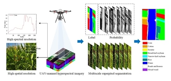
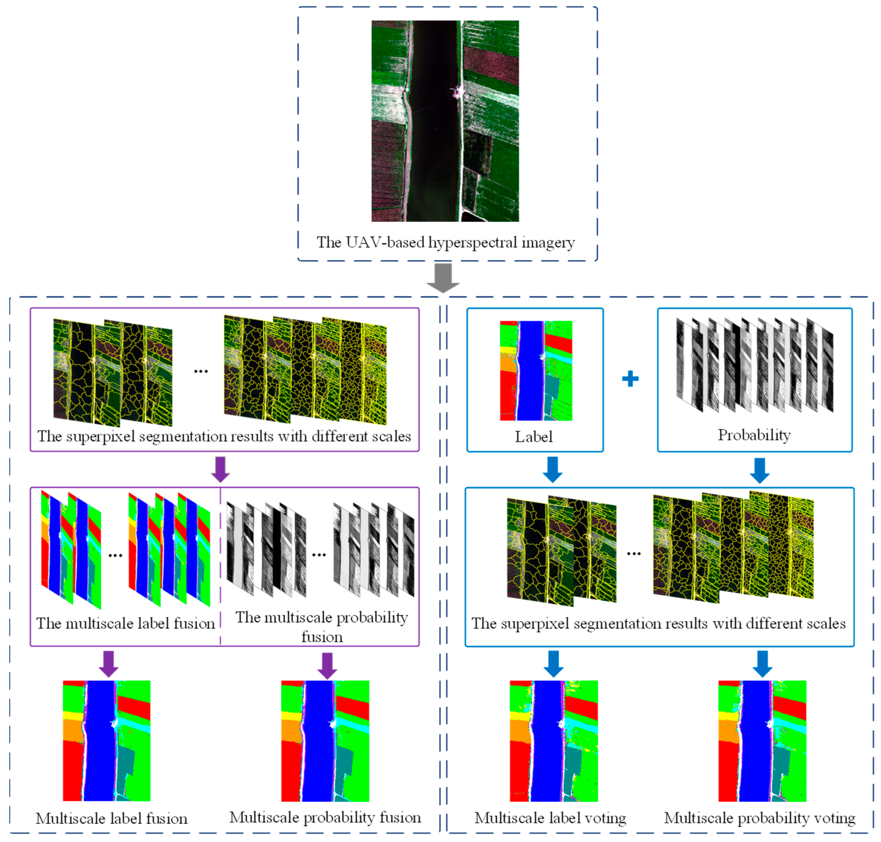
Figure 1.
Flow chart of the research.
Figure 1.
Flow chart of the research.
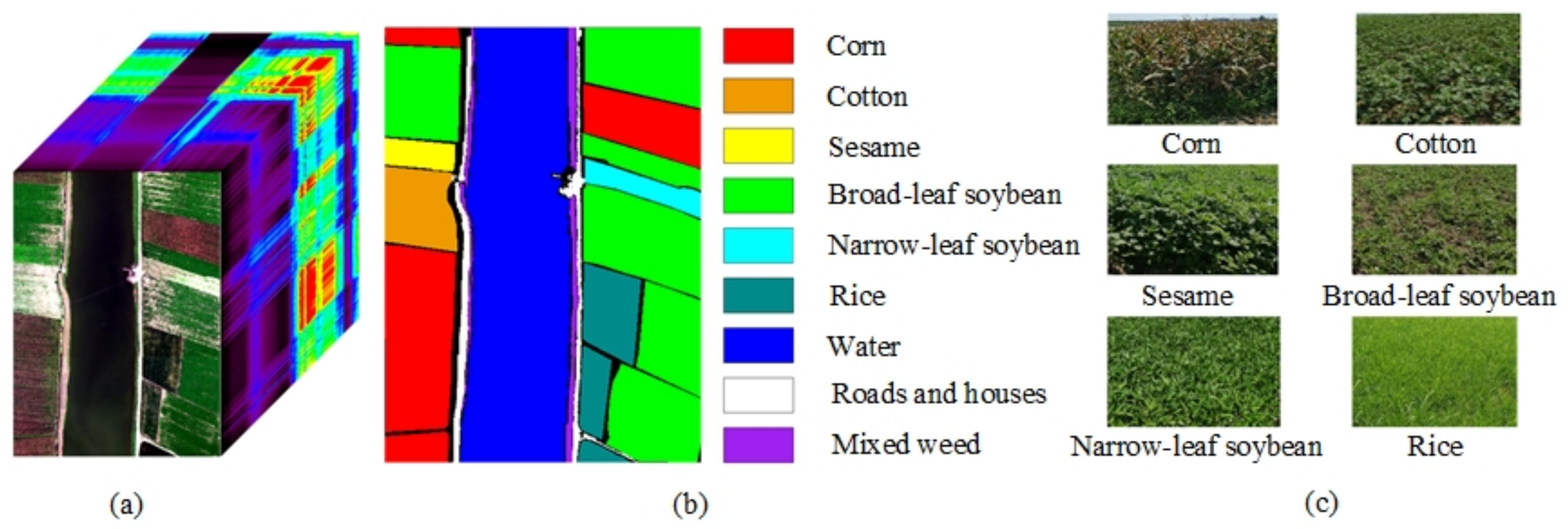
Figure 2.
The LongKou dataset: (a) Hyperspectral image; (b) Ground truth; (c) Typical crop photos in the study area.
Figure 2.
The LongKou dataset: (a) Hyperspectral image; (b) Ground truth; (c) Typical crop photos in the study area.
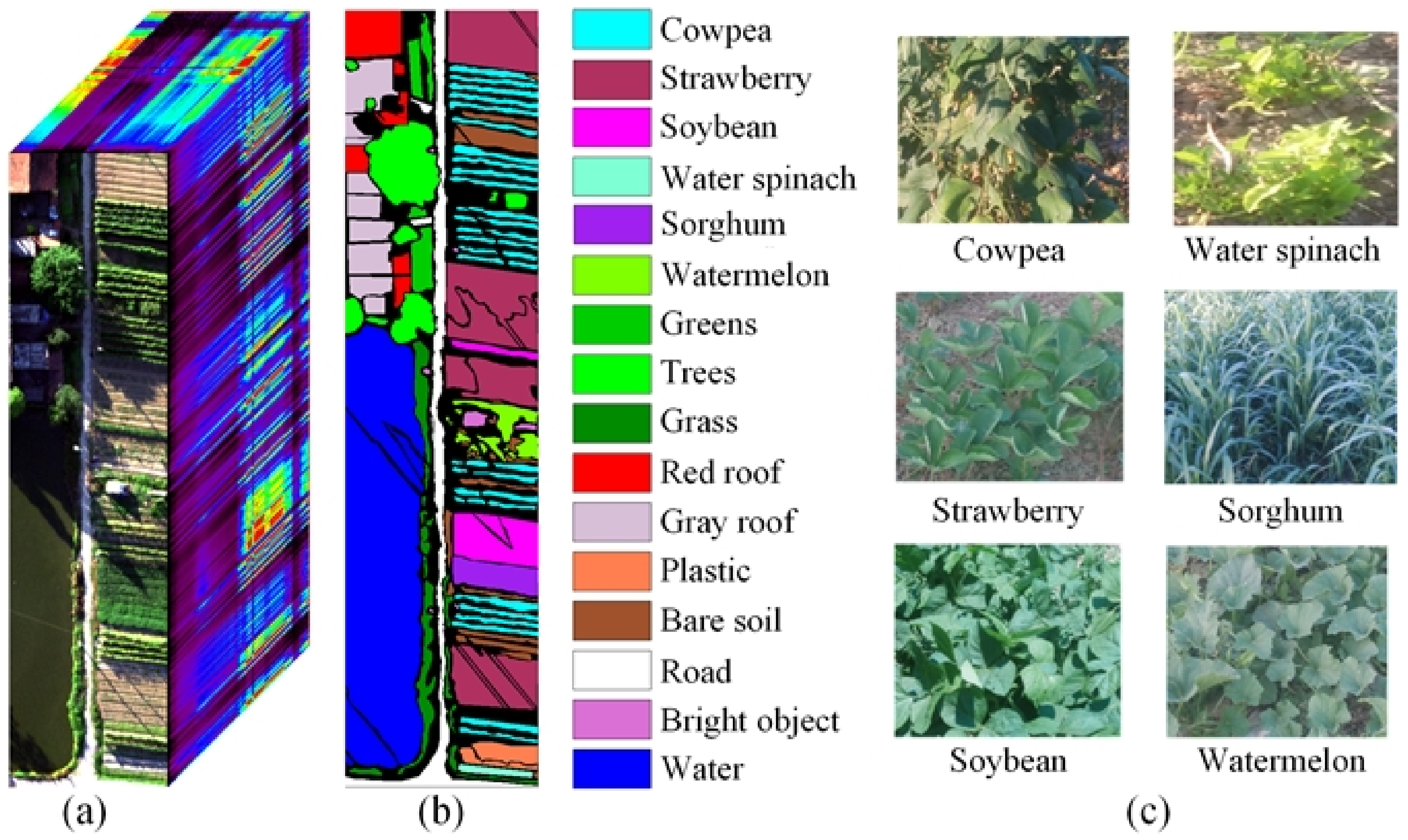
Figure 3.
The HanChuan dataset: (a) Hyperspectral image; (b) Ground truth; (c) Typical crop photos in the study area.
Figure 3.
The HanChuan dataset: (a) Hyperspectral image; (b) Ground truth; (c) Typical crop photos in the study area.
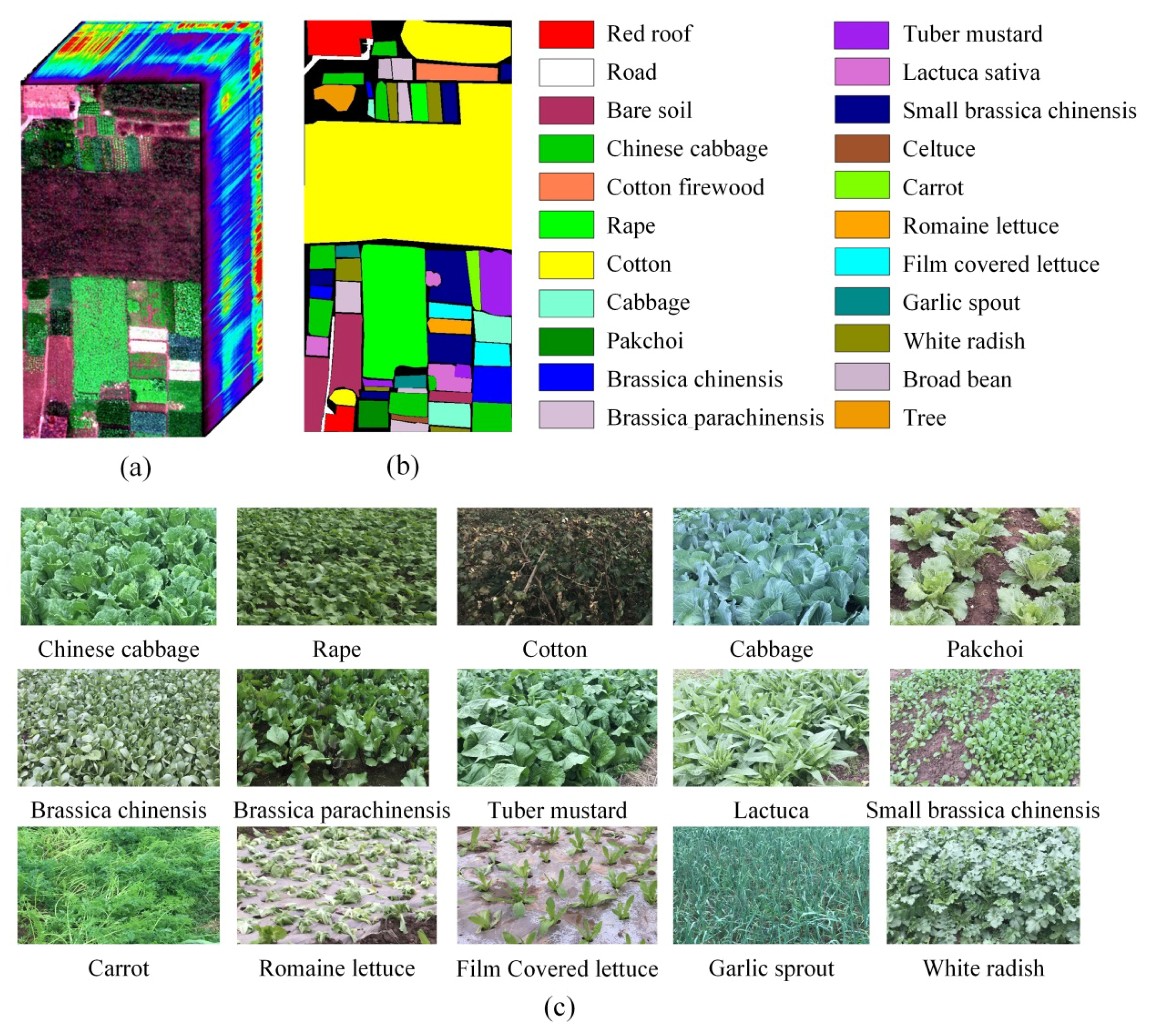
Figure 4.
The HongHu dataset: (a) Hyperspectral image; (b) Ground truth; (c) Typical crop photos in the study area.
Figure 4.
The HongHu dataset: (a) Hyperspectral image; (b) Ground truth; (c) Typical crop photos in the study area.
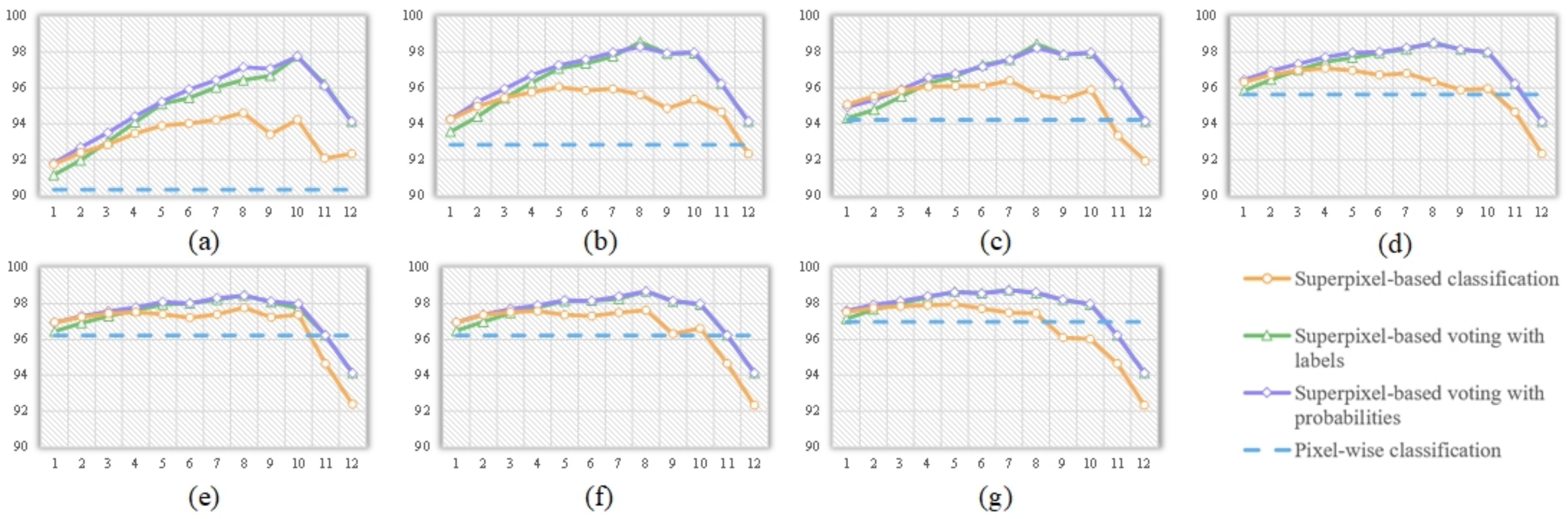
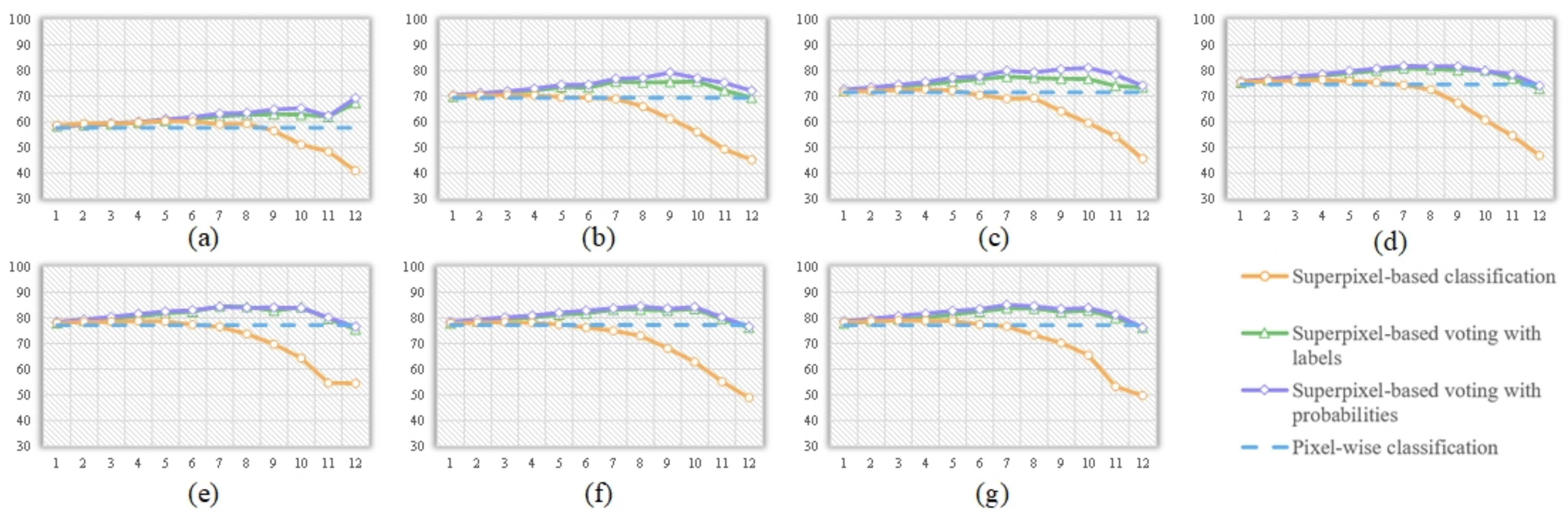
Figure 5.
Accuracies given by the single-scale approaches with (a) 25, (b) 50, (c) 100, (d) 150, (e) 200, (f) 250, and (g) 300 training samples per class for the Longkou dataset using SVM, where the vertical axis represents the OAs, and the horizontal axis represents the superpixel segmentation scale.
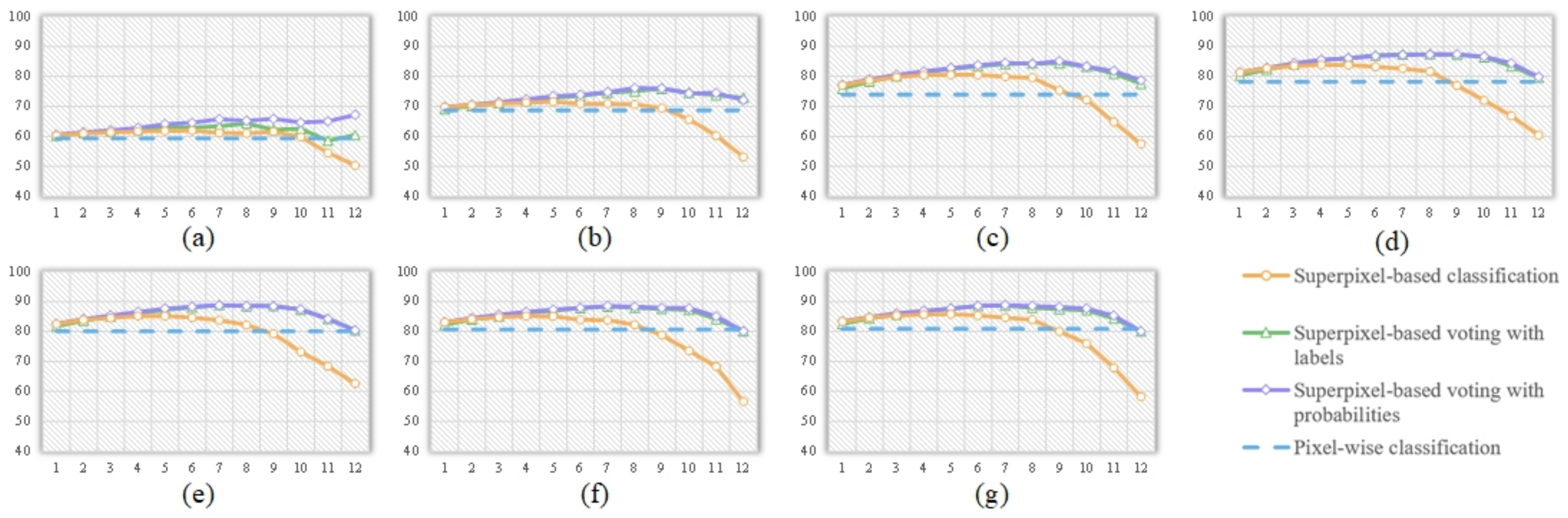
Figure 6.
Accuracies given by the single-scale approaches with (a) 25, (b) 50, (c) 100, (d) 150, (e) 200, (f) 250, and (g) 300 training samples per class for the Hanchuan dataset using SVM, where the vertical axis represents the OAs, and the horizontal axis represents the superpixel segmentation scale.
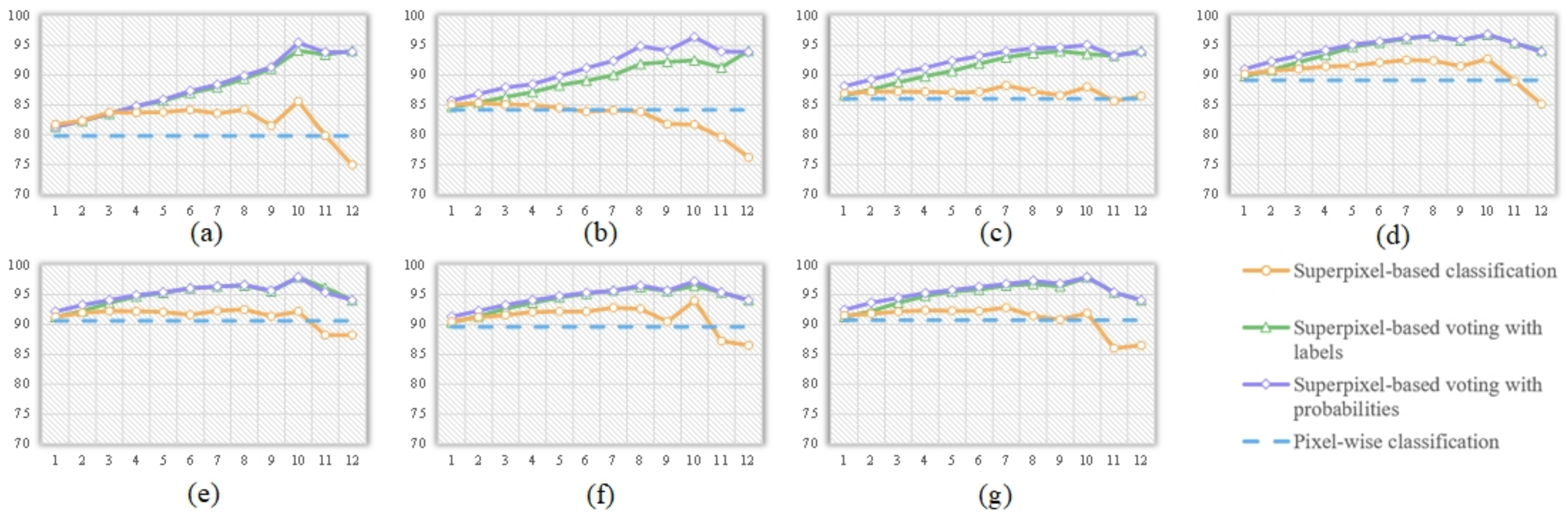
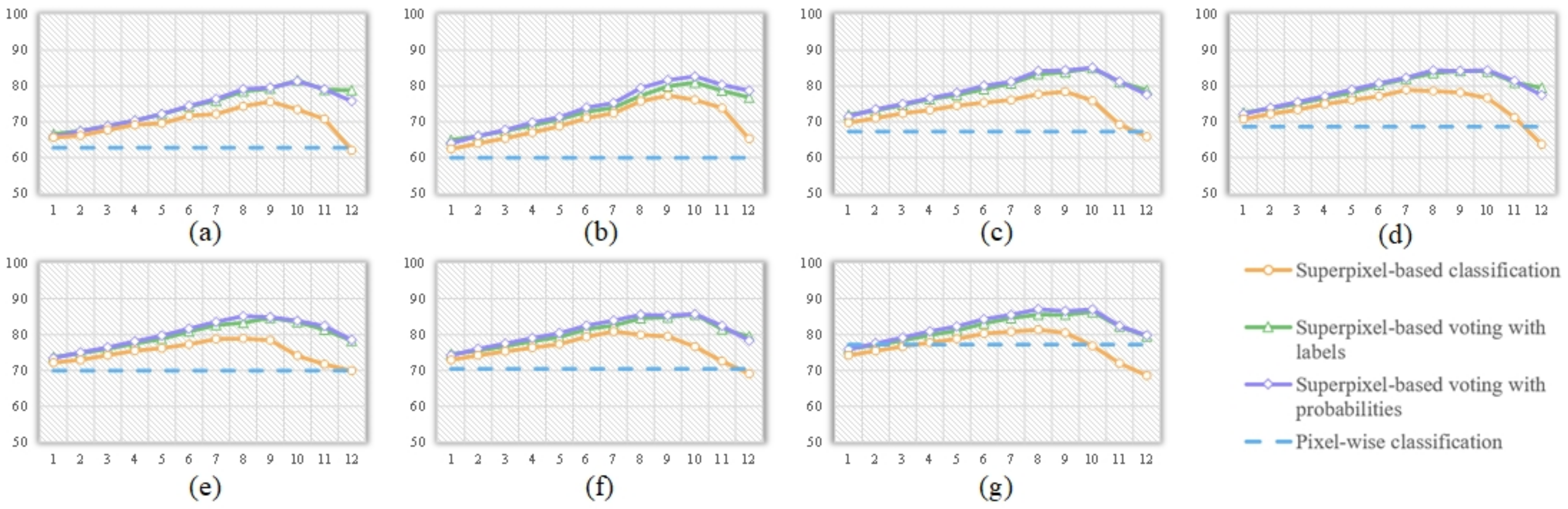
Figure 7.
Accuracies given by the single-scale approaches with (a) 25, (b) 50, (c) 100, (d) 150, (e) 200, (f) 250, and (g) 300 training samples per class for the Honghu dataset using SVM, where the vertical axis represents the OAs, and the horizontal axis represents the superpixel segmentation scale.
Figure 8.
Accuracies given by the single-scale approaches with (a) 25, (b) 50, (c) 100, (d) 150, (e) 200, (f) 250, and (g) 300 training samples per class for the Longkou dataset using RF, where the vertical axis represents the OAs, and the horizontal axis represents the superpixel segmentation scale.
Figure 9.
Accuracies given by the single-scale approaches with (a) 25, (b) 50, (c) 100, (d) 150, (e) 200, (f) 250, and (g) 300 training samples per class for the Hanchuan dataset using RF, where the vertical axis represents the OAs, and the horizontal axis represents the superpixel segmentation scale.
Figure 10.
Accuracies given by the single-scale approaches with (a) 25, (b) 50, (c) 100, (d) 150, (e) 200, (f) 250, and (g) 300 training samples per class for the Honghu dataset using RF, where the vertical axis represents the OAs, and the horizontal axis represents the superpixel segmentation scale.
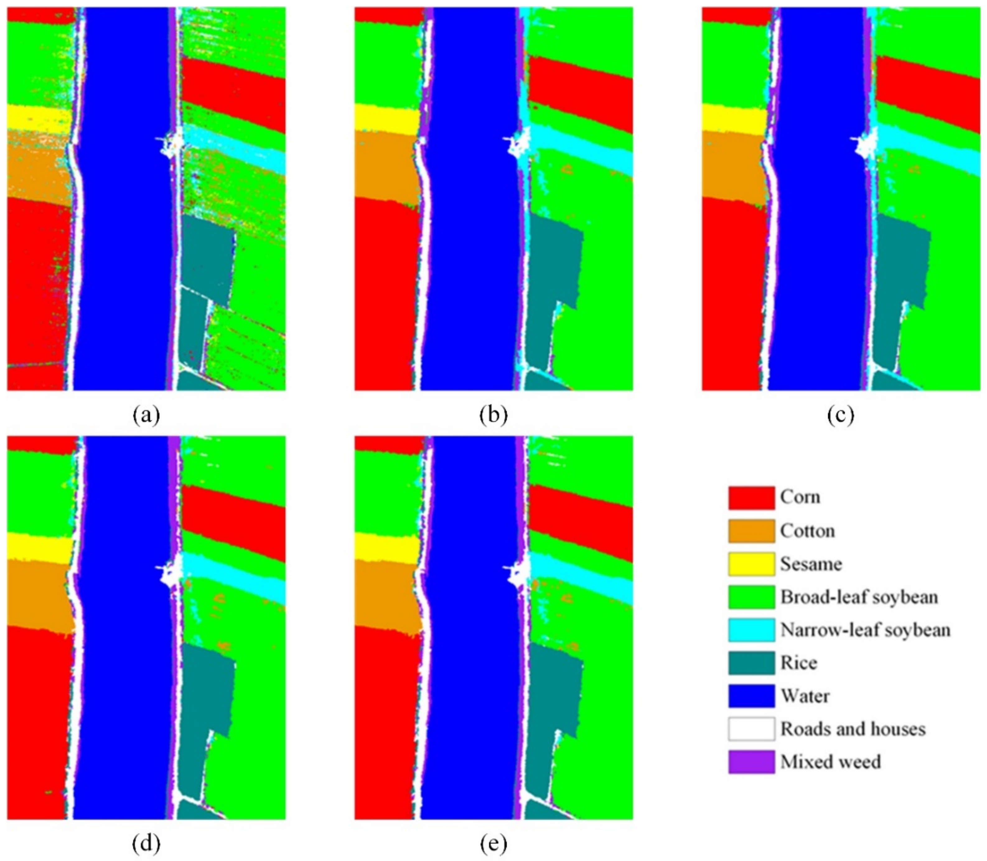
Figure 11.
The classification results for the Longkou dataset using SVM: (a) Pixel-wise spectral classification; (b) MLF; (c) MPF; (d) MLV; (e) MPV.
Figure 11.
The classification results for the Longkou dataset using SVM: (a) Pixel-wise spectral classification; (b) MLF; (c) MPF; (d) MLV; (e) MPV.
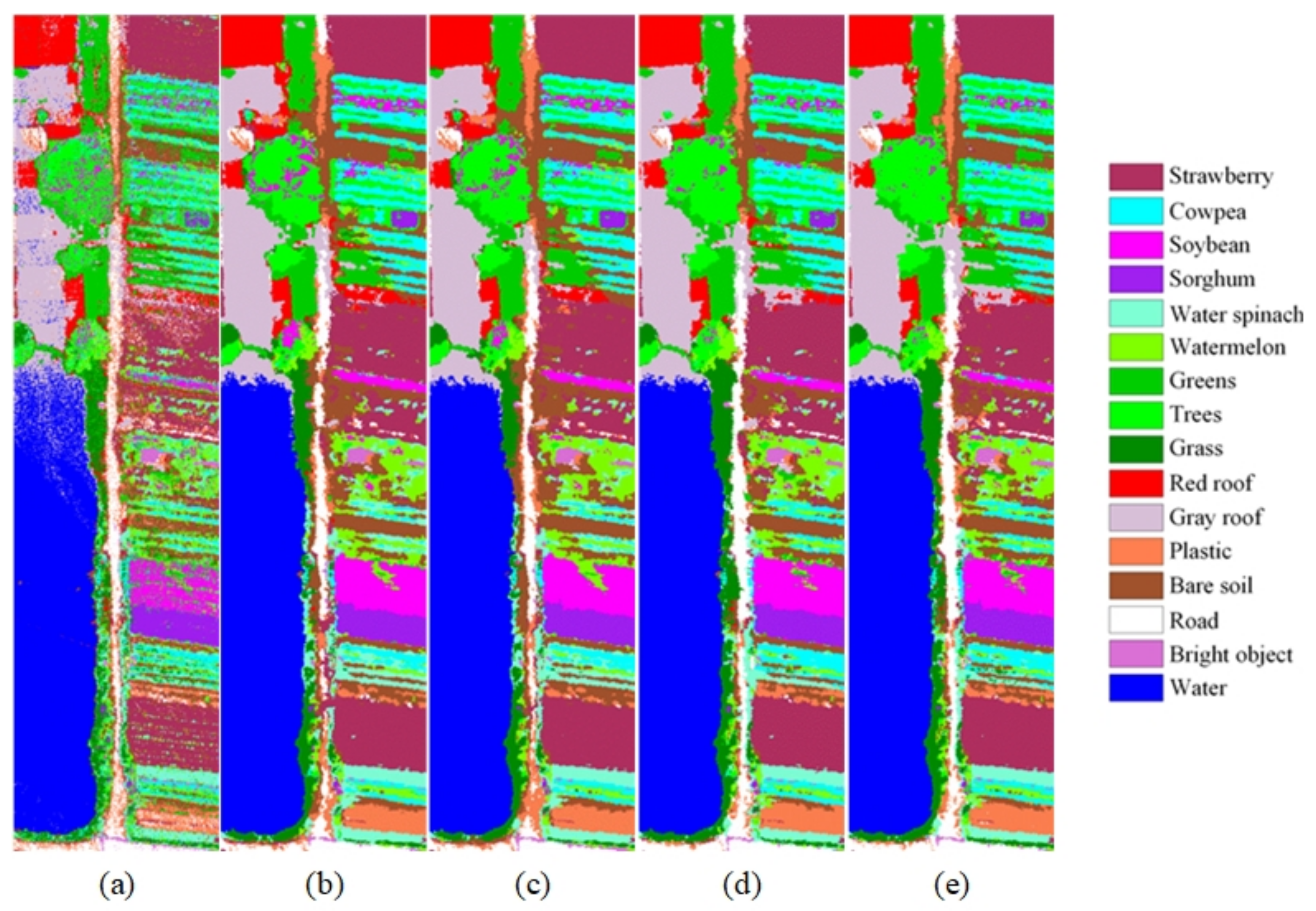
Figure 12.
The classification results for the Hanchuan dataset using SVM: (a) Pixel-wise spectral classification; (b) MLF; (c) MPF; (d) MLV; (e) MPV.
Figure 12.
The classification results for the Hanchuan dataset using SVM: (a) Pixel-wise spectral classification; (b) MLF; (c) MPF; (d) MLV; (e) MPV.
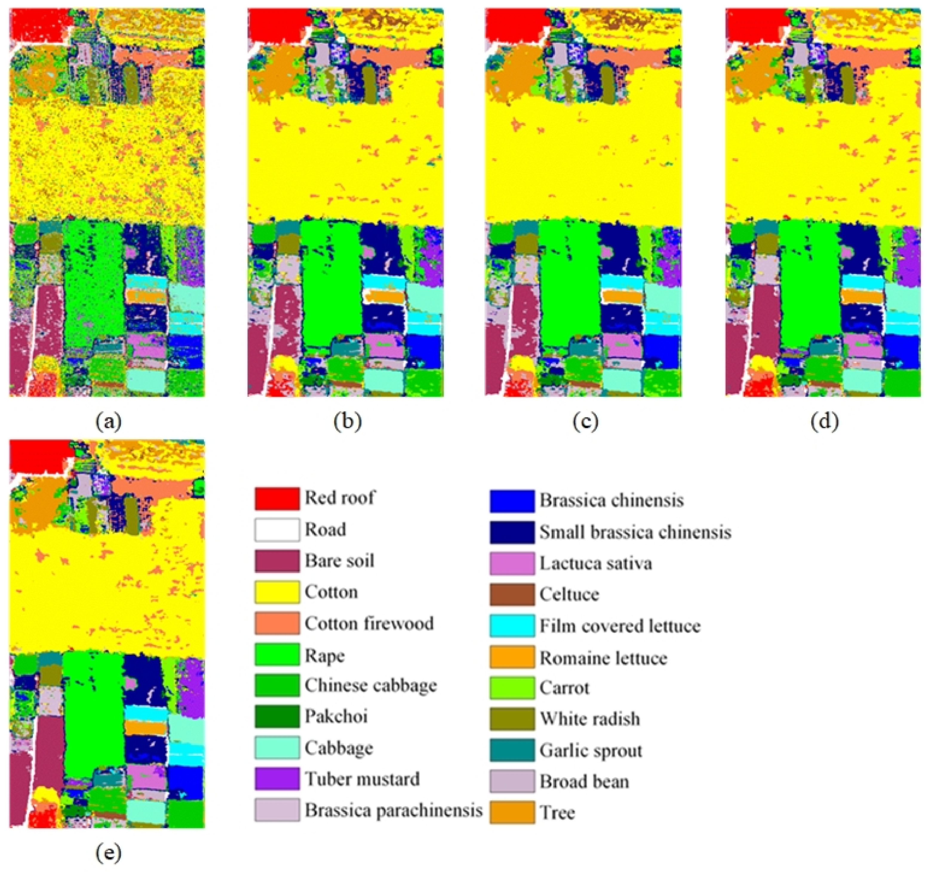
Figure 13.
The classification results for the Honghu dataset using SVM: (a) Pixel-wise spectral classification; (b) MLF; (c) MPF; (d) MLV; (e) MPV.
Figure 13.
The classification results for the Honghu dataset using SVM: (a) Pixel-wise spectral classification; (b) MLF; (c) MPF; (d) MLV; (e) MPV.
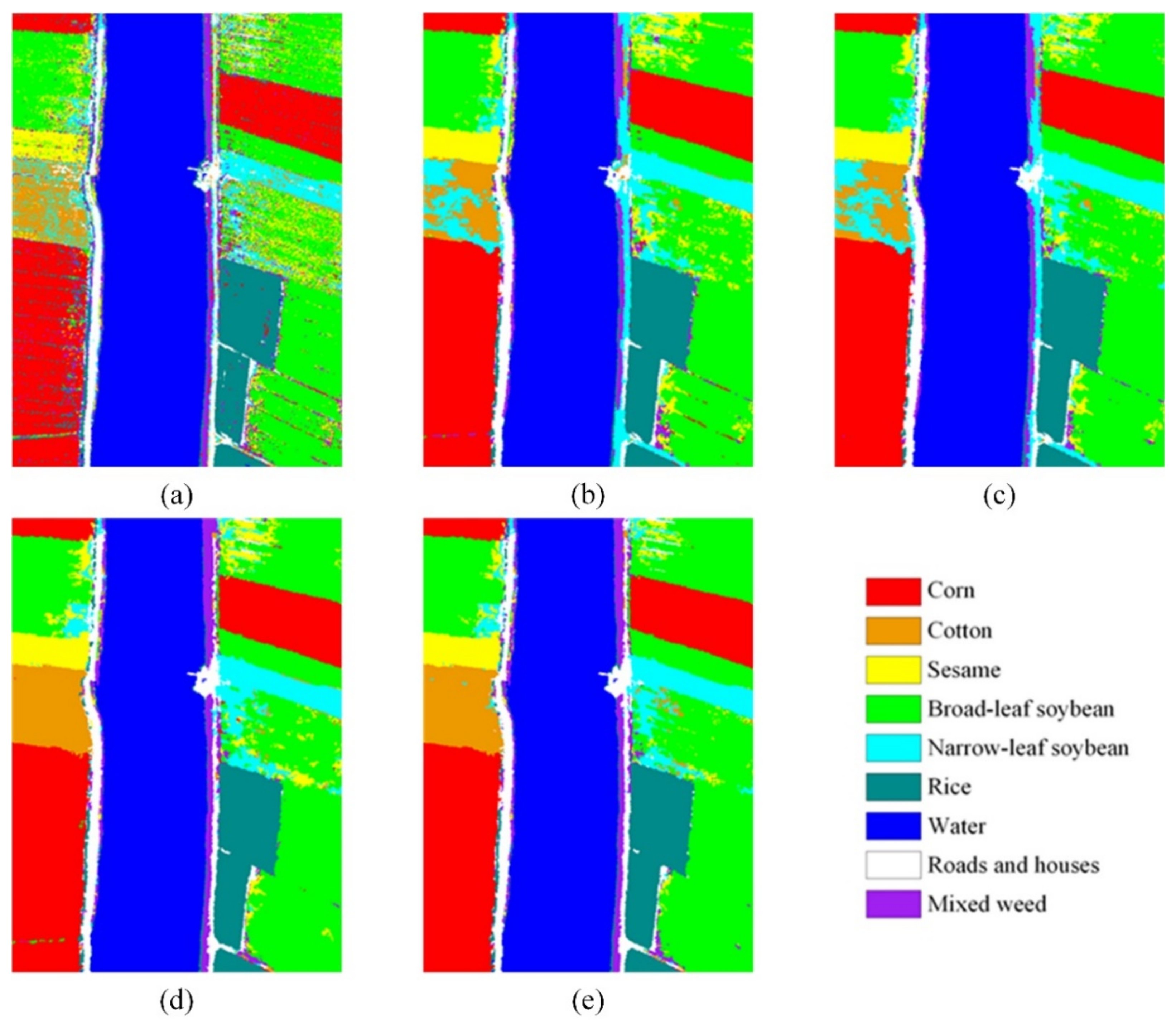
Figure 14.
The classification results for the Longkou dataset using RF: (a) Pixel-wise spectral classification; (b) MLF; (c) MPF; (d) MLV; (e) MPV.
Figure 14.
The classification results for the Longkou dataset using RF: (a) Pixel-wise spectral classification; (b) MLF; (c) MPF; (d) MLV; (e) MPV.
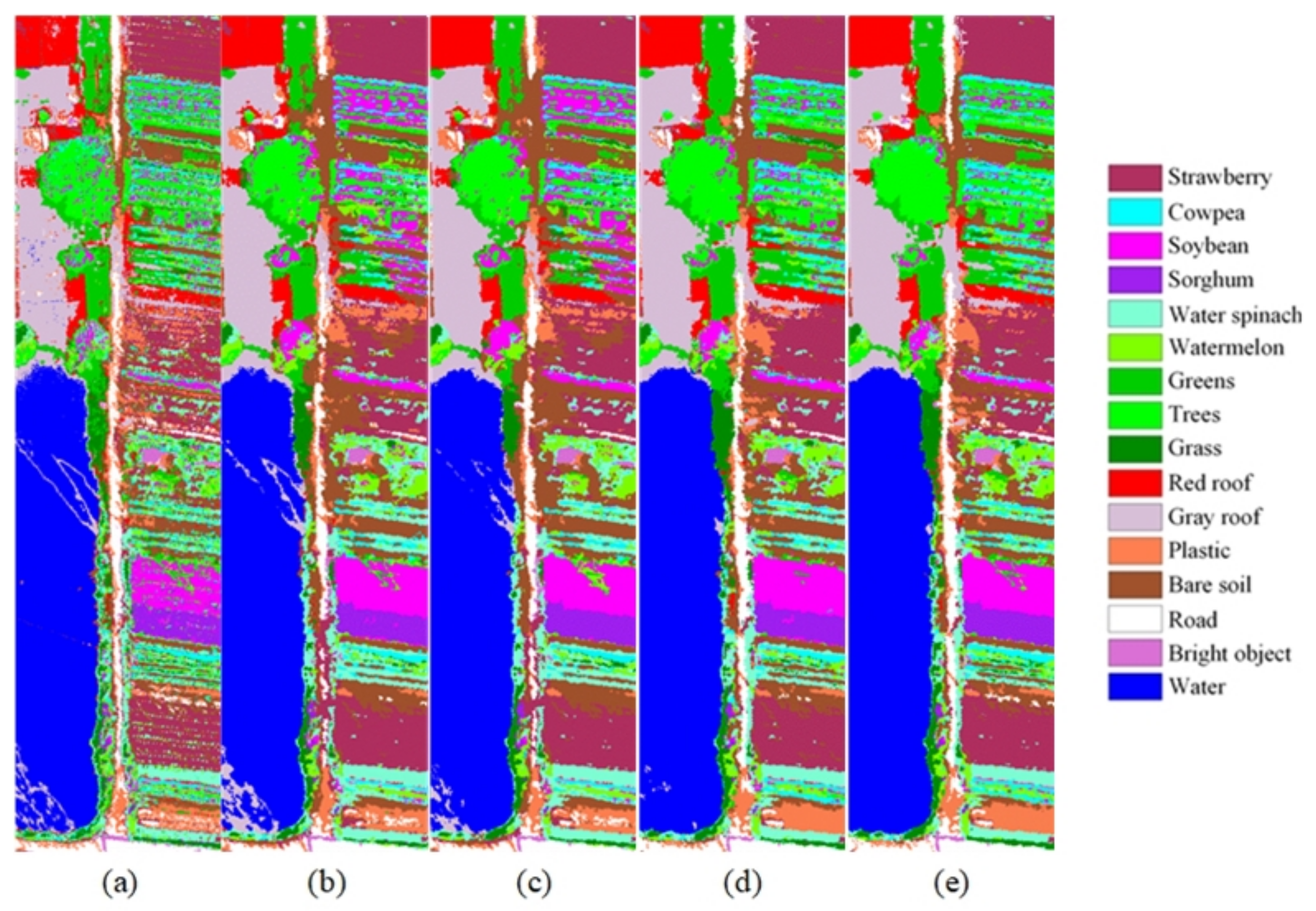
Figure 15.
The classification results for the Hanchuan dataset using RF: (a) Pixel-wise spectral classification; (b) MLF; (c) MPF; (d) MLV; (e) MPV.
Figure 15.
The classification results for the Hanchuan dataset using RF: (a) Pixel-wise spectral classification; (b) MLF; (c) MPF; (d) MLV; (e) MPV.
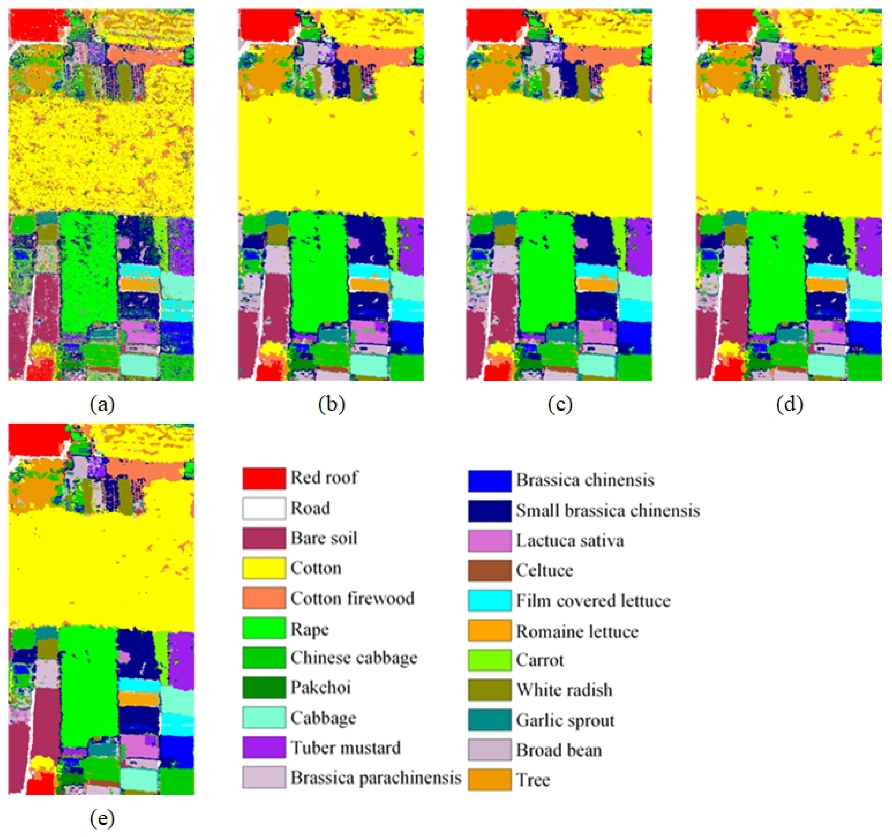
Figure 16.
The classification results for the Honghu dataset using RF: (a) Pixel-wise spectral classification; (b) MLF; (c) MPF; (d) MLV; (e) MPV.
Figure 16.
The classification results for the Honghu dataset using RF: (a) Pixel-wise spectral classification; (b) MLF; (c) MPF; (d) MLV; (e) MPV.
Table 1.
Ground truth classes for the LongKou dataset and the corresponding sample number.
Table 1.
Ground truth classes for the LongKou dataset and the corresponding sample number.
| No. | Class Name | Samples |
|---|
| C1 | Corn | 34,511 |
| C2 | Cotton | 8374 |
| C3 | Sesame | 3031 |
| C4 | Broad-leaf soybean | 63,212 |
| C5 | Narrow-leaf soybean | 4151 |
| C6 | Rice | 11,854 |
| C7 | Water | 67,056 |
| C8 | Roads and houses | 7124 |
| C9 | Mixed weed | 5229 |
Table 2.
Ground truth classes for the HanChuan dataset and the corresponding sample number.
Table 2.
Ground truth classes for the HanChuan dataset and the corresponding sample number.
| No. | Class Name | Samples |
|---|
| C1 | Strawberry | 44,735 |
| C2 | Cowpea | 22,753 |
| C3 | Soybean | 10,287 |
| C4 | Sorghum | 5353 |
| C5 | Water spinach | 1200 |
| C6 | Watermelon | 4533 |
| C7 | Greens | 5903 |
| C8 | Trees | 17,978 |
| C9 | Grass | 9469 |
| C10 | Red roof | 10,516 |
| C11 | Gray roof | 16,911 |
| C12 | Plastic | 3679 |
| C13 | Bare soil | 9116 |
| C14 | Road | 18,560 |
| C15 | Bright object | 1136 |
| C16 | Water | 75,401 |
Table 3.
Ground truth classes for the Honghu dataset and the corresponding sample number.
Table 3.
Ground truth classes for the Honghu dataset and the corresponding sample number.
| No. | Class Name | Samples |
|---|
| C1 | Red roof | 14,041 |
| C2 | Road | 3512 |
| C3 | Bare soil | 21,821 |
| C4 | Cotton | 163,285 |
| C5 | Cotton firewood | 6218 |
| C6 | Rape | 44,557 |
| C7 | Chinese cabbage | 24,103 |
| C8 | Pakchoi | 4054 |
| C9 | Cabbage | 10,819 |
| C10 | Tuber mustard | 12,394 |
| C11 | Brassica parachinensis | 11,015 |
| C12 | Brassica chinensis | 8954 |
| C13 | Small Brassica chinensis | 22,507 |
| C14 | Lactuca sativa | 7356 |
| C15 | Celtuce | 1002 |
| C16 | Film covered lettuce | 7262 |
| C17 | Romaine lettuce | 3010 |
| C18 | Carrot | 3217 |
| C19 | White radish | 8712 |
| C20 | Garlic sprout | 3486 |
Table 4.
OAs (%) and Kappa coefficients obtained by different methods for the Longkou dataset using SVM with different numbers of training samples per class.
Table 4.
OAs (%) and Kappa coefficients obtained by different methods for the Longkou dataset using SVM with different numbers of training samples per class.
| Training Samples | Spectral | MLF | MPF | MLV | MPV |
|---|
| OA | Kappa | OA | Kappa | OA | Kappa | OA | Kappa | OA | Kappa |
|---|
| 25 | 90.32 | 0.875 | 95.42 | 0.940 | 96.09 | 0.949 | 97.18 | 0.963 | 97.54 | 0.968 |
| 50 | 92.83 | 0.907 | 97.15 | 0.963 | 97.79 | 0.971 | 98.70 | 0.983 | 98.96 | 0.986 |
| 100 | 94.22 | 0.925 | 97.44 | 0.966 | 97.94 | 0.973 | 98.47 | 0.980 | 98.52 | 0.981 |
| 150 | 95.64 | 0.943 | 97.75 | 0.970 | 98.38 | 0.979 | 98.91 | 0.986 | 99.03 | 0.987 |
| 200 | 96.17 | 0.950 | 98.47 | 0.980 | 98.87 | 0.985 | 98.85 | 0.985 | 99.07 | 0.988 |
| 250 | 96.23 | 0.951 | 98.43 | 0.979 | 98.86 | 0.985 | 99.08 | 0.988 | 99.21 | 0.990 |
| 300 | 96.98 | 0.961 | 98.68 | 0.983 | 98.99 | 0.987 | 99.27 | 0.990 | 99.33 | 0.991 |
Table 5.
OAs (%) and Kappa coefficients obtained by different methods for the Hanchuan dataset using SVM with different numbers of training samples per class.
Table 5.
OAs (%) and Kappa coefficients obtained by different methods for the Hanchuan dataset using SVM with different numbers of training samples per class.
| Training Samples | Spectral | MLF | MPF | MLV | MPV |
|---|
| OA | Kappa | OA | Kappa | OA | Kappa | OA | Kappa | OA | Kappa |
|---|
| 25 | 59.28 | 0.541 | 63.06 | 0.583 | 64.36 | 0.597 | 64.43 | 0.598 | 66.60 | 0.622 |
| 50 | 68.67 | 0.643 | 73.30 | 0.695 | 75.04 | 0.715 | 76.65 | 0.733 | 77.09 | 0.738 |
| 100 | 73.93 | 0.700 | 82.91 | 0.802 | 83.15 | 0.805 | 86.41 | 0.842 | 86.21 | 0.840 |
| 150 | 78.24 | 0.749 | 85.59 | 0.833 | 86.23 | 0.840 | 89.75 | 0.881 | 89.65 | 0.880 |
| 200 | 80.08 | 0.770 | 87.06 | 0.850 | 87.48 | 0.855 | 90.88 | 0.894 | 90.67 | 0.891 |
| 250 | 80.66 | 0.776 | 86.64 | 0.845 | 87.02 | 0.849 | 90.47 | 0.889 | 90.68 | 0.892 |
| 300 | 80.89 | 0.779 | 87.77 | 0.858 | 87.96 | 0.860 | 90.64 | 0.891 | 90.79 | 0.893 |
Table 6.
OAs (%) and Kappa coefficients obtained by different methods for the Honghu dataset using SVM with different numbers of training samples per class.
Table 6.
OAs (%) and Kappa coefficients obtained by different methods for the Honghu dataset using SVM with different numbers of training samples per class.
| Training Samples | Spectral | MLF | MPF | MLV | MPV |
|---|
| OA | Kappa | OA | Kappa | OA | Kappa | OA | Kappa | OA | Kappa |
|---|
| 25 | 66.98 | 0.605 | 81.51 | 0.770 | 82.56 | 0.783 | 83.93 | 0.799 | 83.39 | 0.794 |
| 50 | 64.08 | 0.581 | 82.16 | 0.779 | 83.35 | 0.793 | 81.63 | 0.774 | 81.80 | 0.777 |
| 100 | 73.42 | 0.681 | 88.26 | 0.853 | 88.74 | 0.859 | 88.87 | 0.861 | 89.31 | 0.866 |
| 150 | 74.74 | 0.695 | 88.50 | 0.856 | 88.90 | 0.861 | 89.71 | 0.871 | 90.06 | 0.876 |
| 200 | 77.05 | 0.721 | 90.24 | 0.877 | 90.65 | 0.882 | 90.87 | 0.885 | 91.05 | 0.888 |
| 250 | 77.43 | 0.726 | 90.80 | 0.884 | 91.28 | 0.890 | 91.70 | 0.896 | 91.86 | 0.898 |
| 300 | 79.77 | 0.752 | 90.88 | 0.885 | 91.06 | 0.887 | 92.07 | 0.900 | 92.40 | 0.904 |
Table 7.
OAs (%) and Kappa coefficients obtained by different methods for the Longkou dataset using RF with different numbers of training samples per class.
Table 7.
OAs (%) and Kappa coefficients obtained by different methods for the Longkou dataset using RF with different numbers of training samples per class.
| Training Samples | Spectral | MLF | MPF | MLV | MPV |
|---|
| OA | Kappa | OA | Kappa | OA | Kappa | OA | Kappa | OA | Kappa |
|---|
| 25 | 79.79 | 0.746 | 86.10 | 0.823 | 87.17 | 0.837 | 91.08 | 0.886 | 91.31 | 0.888 |
| 50 | 84.14 | 0.799 | 85.10 | 0.812 | 87.14 | 0.837 | 92.02 | 0.898 | 94.69 | 0.931 |
| 100 | 86.03 | 0.823 | 89.84 | 0.870 | 91.60 | 0.892 | 93.80 | 0.920 | 95.33 | 0.940 |
| 150 | 89.15 | 0.861 | 94.32 | 0.926 | 94.54 | 0.929 | 97.07 | 0.962 | 97.13 | 0.963 |
| 200 | 90.67 | 0.880 | 94.41 | 0.927 | 94.85 | 0.933 | 97.47 | 0.967 | 97.42 | 0.966 |
| 250 | 89.64 | 0.867 | 94.38 | 0.927 | 94.77 | 0.932 | 96.83 | 0.959 | 97.14 | 0.963 |
| 300 | 90.76 | 0.881 | 94.02 | 0.922 | 94.74 | 0.932 | 97.48 | 0.967 | 97.75 | 0.971 |
Table 8.
OAs (%) and Kappa coefficients obtained by different methods for the Hanchuan dataset using RF with different numbers of training samples per class.
Table 8.
OAs (%) and Kappa coefficients obtained by different methods for the Hanchuan dataset using RF with different numbers of training samples per class.
| Training Samples | Spectral | MLF | MPF | MLV | MPV |
|---|
| OA | Kappa | OA | Kappa | OA | Kappa | OA | Kappa | OA | Kappa |
|---|
| 25 | 57.69 | 0.524 | 62.69 | 0.578 | 63.03 | 0.582 | 64.55 | 0.599 | 64.54 | 0.599 |
| 50 | 69.38 | 0.649 | 71.36 | 0.671 | 72.73 | 0.686 | 76.98 | 0.734 | 78.49 | 0.751 |
| 100 | 71.46 | 0.673 | 74.00 | 0.702 | 75.64 | 0.720 | 79.62 | 0.765 | 81.03 | 0.781 |
| 150 | 74.61 | 0.708 | 78.41 | 0.751 | 79.45 | 0.762 | 82.72 | 0.800 | 83.53 | 0.809 |
| 200 | 77.19 | 0.736 | 80.26 | 0.771 | 80.91 | 0.779 | 85.96 | 0.837 | 86.16 | 0.839 |
| 250 | 77.24 | 0.737 | 79.27 | 0.760 | 80.03 | 0.769 | 85.44 | 0.831 | 85.98 | 0.837 |
| 300 | 77.15 | 0.736 | 79.93 | 0.768 | 81.19 | 0.782 | 85.23 | 0.829 | 86.24 | 0.840 |
Table 9.
OAs (%) and Kappa coefficients obtained by different methods for the Honghu dataset using RF with different numbers of training samples per class.
Table 9.
OAs (%) and Kappa coefficients obtained by different methods for the Honghu dataset using RF with different numbers of training samples per class.
| Training Samples | Spectral | MLF | MPF | MLV | MPV |
|---|
| OA | Kappa | OA | Kappa | OA | Kappa | OA | Kappa | OA | Kappa |
|---|
| 25 | 62.79 | 0.559 | 76.74 | 0.713 | 78.15 | 0.730 | 79.50 | 0.745 | 78.56 | 0.736 |
| 50 | 59.99 | 0.537 | 77.75 | 0.727 | 78.69 | 0.738 | 78.57 | 0.739 | 78.47 | 0.739 |
| 100 | 67.28 | 0.612 | 80.64 | 0.760 | 82.53 | 0.783 | 83.63 | 0.797 | 84.08 | 0.803 |
| 150 | 68.60 | 0.626 | 81.69 | 0.773 | 82.43 | 0.782 | 84.47 | 0.807 | 84.48 | 0.808 |
| 200 | 69.96 | 0.640 | 82.12 | 0.778 | 82.46 | 0.782 | 84.75 | 0.810 | 85.69 | 0.822 |
| 250 | 70.44 | 0.646 | 83.16 | 0.791 | 84.05 | 0.802 | 85.32 | 0.817 | 86.45 | 0.832 |
| 300 | 72.08 | 0.664 | 83.76 | 0.798 | 84.42 | 0.806 | 86.60 | 0.833 | 87.71 | 0.847 |
Table 10.
Classification accuracies given by different methods for the Longkou dataset using SVM and RF with 100 training samples per class.
Table 10.
Classification accuracies given by different methods for the Longkou dataset using SVM and RF with 100 training samples per class.
| No. | SVM | RF |
|---|
| | Spectral | MLF | MPF | MLV | MPV | Spectral | MLF | MPF | MLV | MPV |
|---|
| C1 | 97.66 | 99.51 | 99.54 | 99.53 | 99.55 | 93.28 | 99.14 | 99.48 | 99.44 | 99.55 |
| C2 | 79.16 | 97.08 | 97.81 | 95.96 | 96.04 | 68.39 | 68.17 | 68.25 | 97.09 | 95.37 |
| C3 | 73.64 | 97.31 | 99.00 | 97.49 | 97.90 | 33.07 | 45.04 | 56.06 | 52.03 | 69.91 |
| C4 | 92.21 | 98.18 | 98.55 | 98.19 | 98.10 | 81.64 | 88.90 | 91.50 | 90.19 | 92.86 |
| C5 | 72.65 | 71.20 | 75.02 | 90.04 | 89.39 | 51.38 | 43.89 | 44.52 | 63.97 | 65.75 |
| C6 | 98.44 | 98.91 | 98.88 | 99.15 | 99.21 | 90.44 | 98.15 | 98.57 | 98.85 | 98.61 |
| C7 | 99.96 | 99.96 | 99.96 | 99.96 | 99.96 | 99.95 | 99.96 | 99.96 | 99.95 | 99.95 |
| C8 | 88.15 | 83.72 | 85.38 | 94.37 | 95.24 | 84.91 | 79.55 | 82.13 | 91.99 | 93.48 |
| C9 | 85.16 | 84.71 | 90.89 | 91.84 | 93.89 | 59.24 | 67.55 | 77.62 | 86.38 | 87.67 |
| OA | 94.22 | 97.44 | 97.94 | 98.47 | 98.52 | 86.03 | 89.84 | 91.60 | 93.80 | 95.33 |
| Kappa | 0.925 | 0.966 | 0.973 | 0.980 | 0.981 | 0.823 | 0.870 | 0.892 | 0.920 | 0.940 |
Table 11.
Classification accuracies given by different methods for the Hanchuan dataset using SVM and RF with 100 training samples per class.
Table 11.
Classification accuracies given by different methods for the Hanchuan dataset using SVM and RF with 100 training samples per class.
| No. | SVM | RF |
|---|
| | Spectral | MLF | MPF | MLV | MPV | Spectral | MLF | MPF | MLV | MPV |
|---|
| C1 | 78.83 | 90.95 | 91.59 | 92.66 | 92.09 | 74.45 | 81.98 | 84.30 | 86.96 | 87.37 |
| C2 | 60.19 | 72.79 | 73.71 | 81.51 | 78.99 | 44.52 | 41.14 | 42.44 | 55.55 | 60.12 |
| C3 | 64.99 | 78.88 | 80.58 | 88.49 | 88.51 | 62.62 | 61.74 | 61.14 | 75.57 | 78.15 |
| C4 | 87.91 | 91.43 | 91.66 | 91.61 | 92.67 | 82.06 | 92.27 | 94.86 | 93.52 | 95.45 |
| C5 | 25.04 | 25.74 | 28.46 | 39.83 | 41.60 | 18.65 | 17.92 | 18.61 | 22.03 | 25.00 |
| C6 | 28.57 | 51.90 | 53.21 | 55.93 | 55.84 | 23.28 | 36.14 | 42.73 | 40.11 | 42.44 |
| C7 | 64.32 | 75.81 | 77.23 | 73.50 | 74.34 | 65.58 | 75.31 | 76.28 | 73.77 | 74.08 |
| C8 | 60.59 | 73.35 | 75.93 | 78.77 | 80.09 | 61.74 | 67.70 | 68.87 | 71.71 | 73.01 |
| C9 | 62.25 | 75.22 | 74.87 | 82.02 | 82.70 | 50.31 | 56.59 | 56.28 | 61.84 | 64.69 |
| C10 | 85.52 | 88.78 | 90.34 | 92.38 | 92.16 | 79.61 | 85.34 | 86.64 | 84.57 | 86.17 |
| C11 | 75.98 | 85.81 | 86.35 | 84.79 | 84.33 | 78.28 | 80.12 | 83.56 | 83.76 | 85.03 |
| C12 | 33.12 | 55.45 | 50.31 | 65.09 | 58.88 | 32.32 | 37.47 | 38.62 | 50.22 | 49.86 |
| C13 | 41.02 | 55.47 | 54.25 | 56.99 | 58.51 | 44.55 | 47.32 | 48.05 | 57.53 | 59.04 |
| C14 | 68.35 | 69.45 | 68.90 | 78.00 | 78.99 | 66.54 | 60.62 | 64.03 | 69.07 | 73.31 |
| C15 | 58.34 | 72.87 | 71.78 | 73.08 | 77.65 | 58.56 | 61.23 | 64.36 | 71.61 | 71.67 |
| C16 | 95.70 | 97.96 | 97.84 | 98.06 | 98.08 | 97.05 | 96.53 | 97.46 | 98.54 | 98.69 |
| OA | 73.93 | 82.91 | 83.15 | 86.41 | 86.21 | 71.46 | 74.00 | 75.64 | 79.62 | 81.03 |
| Kappa | 0.700 | 0.802 | 0.805 | 0.842 | 0.840 | 0.673 | 0.702 | 0.720 | 0.765 | 0.781 |
Table 12.
Classification accuracies given by different methods for the Honghu dataset using SVM and RF with 100 training samples per class.
Table 12.
Classification accuracies given by different methods for the Honghu dataset using SVM and RF with 100 training samples per class.
| No. | SVM | RF |
|---|
| | Spectral | MLF | MPF | MLV | MPV | Spectral | MLF | MPF | MLV | MPV |
|---|
| C1 | 92.20 | 96.01 | 95.90 | 96.73 | 97.37 | 85.09 | 91.06 | 90.74 | 93.78 | 94.31 |
| C2 | 70.67 | 78.46 | 80.86 | 74.72 | 81.43 | 65.80 | 67.89 | 71.36 | 70.53 | 77.66 |
| C3 | 83.69 | 87.96 | 87.61 | 91.34 | 91.68 | 80.79 | 82.25 | 84.30 | 90.16 | 91.08 |
| C4 | 86.04 | 97.93 | 97.91 | 97.07 | 97.05 | 82.06 | 94.92 | 96.10 | 94.25 | 93.57 |
| C5 | 34.13 | 72.91 | 78.04 | 67.70 | 69.78 | 26.02 | 50.26 | 60.04 | 50.97 | 47.77 |
| C6 | 87.15 | 92.92 | 93.53 | 93.69 | 94.16 | 81.96 | 89.03 | 90.33 | 90.80 | 92.48 |
| C7 | 68.43 | 77.39 | 77.86 | 80.53 | 81.07 | 56.80 | 62.95 | 61.55 | 67.51 | 70.17 |
| C8 | 24.83 | 54.03 | 57.93 | 59.51 | 59.15 | 19.43 | 33.24 | 39.23 | 43.20 | 45.94 |
| C9 | 94.55 | 95.58 | 95.49 | 95.87 | 96.13 | 92.11 | 94.73 | 94.99 | 95.94 | 96.15 |
| C10 | 57.51 | 84.56 | 85.29 | 84.38 | 85.89 | 42.71 | 50.35 | 52.68 | 74.86 | 78.58 |
| C11 | 41.06 | 73.91 | 73.23 | 73.82 | 72.99 | 33.37 | 52.18 | 57.80 | 67.53 | 64.05 |
| C12 | 53.33 | 70.30 | 71.64 | 71.53 | 71.38 | 51.89 | 61.94 | 63.36 | 64.82 | 67.93 |
| C13 | 59.75 | 70.38 | 72.71 | 72.08 | 74.06 | 58.60 | 68.62 | 72.61 | 69.54 | 72.22 |
| C14 | 70.24 | 74.01 | 76.56 | 77.16 | 81.97 | 61.34 | 69.22 | 68.60 | 73.30 | 76.48 |
| C15 | 13.66 | 63.98 | 63.89 | 78.17 | 76.22 | 13.62 | 32.29 | 31.13 | 80.04 | 63.29 |
| C16 | 85.03 | 94.67 | 95.18 | 95.85 | 96.28 | 81.64 | 90.01 | 92.72 | 93.85 | 94.81 |
| C17 | 70.28 | 88.99 | 89.70 | 93.41 | 94.33 | 68.13 | 78.13 | 84.79 | 91.22 | 93.47 |
| C18 | 45.13 | 73.34 | 76.86 | 76.17 | 75.62 | 33.28 | 49.41 | 48.18 | 51.45 | 52.33 |
| C19 | 75.09 | 89.08 | 88.87 | 87.49 | 88.25 | 67.27 | 83.61 | 83.23 | 81.09 | 84.80 |
| C20 | 58.31 | 76.98 | 77.50 | 82.70 | 82.63 | 36.62 | 56.63 | 58.68 | 76.96 | 75.15 |
| C21 | 21.25 | 29.08 | 29.77 | 36.58 | 41.69 | 20.39 | 21.20 | 22.54 | 32.80 | 38.83 |
| C22 | 38.83 | 64.57 | 60.78 | 61.94 | 57.14 | 28.63 | 55.37 | 54.76 | 44.54 | 43.38 |
| OA | 73.42 | 88.26 | 88.74 | 88.87 | 89.31 | 67.28 | 80.64 | 82.53 | 83.63 | 84.08 |
| Kappa | 0.681 | 0.853 | 0.859 | 0.861 | 0.866 | 0.612 | 0.760 | 0.783 | 0.797 | 0.803 |


