
Estimating the Applicability of NDVI and SIF to Gross Primary Productivity and Grain-Yield Monitoring in China


Abstract
:
1. Introduction
2. Data and Methods
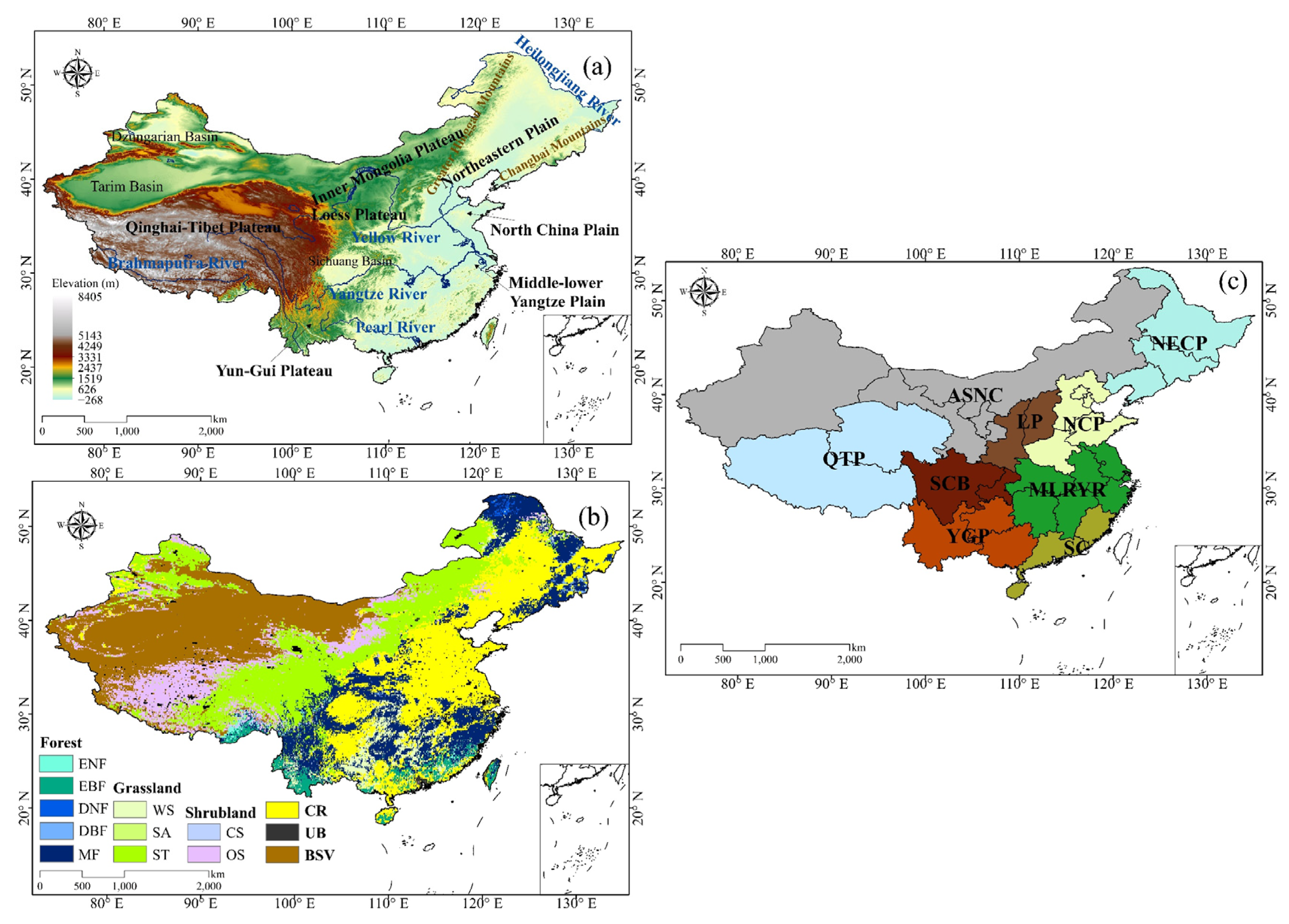
2.1. Study Area
2.2. Datasets
2.3. Analysis
3. Results
3.1. Consistency between SIF and NDVI
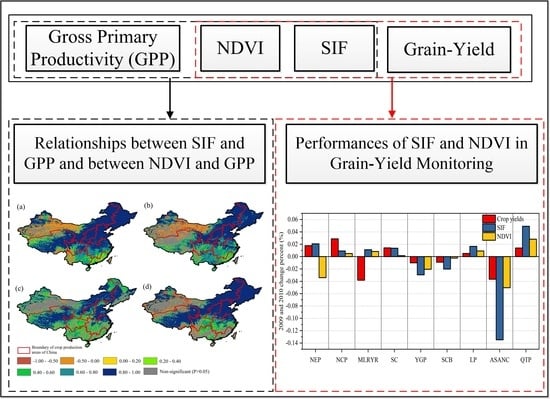
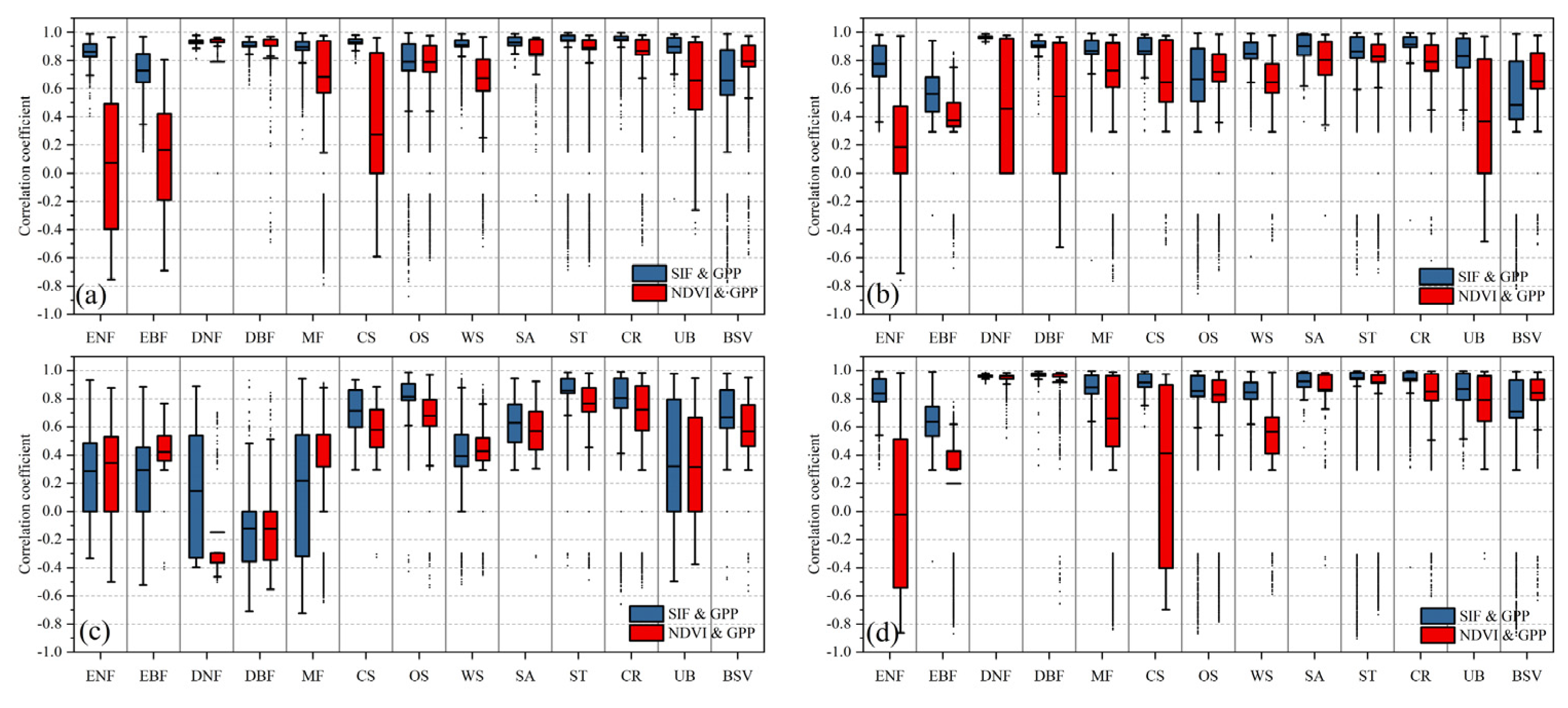
3.2. Relationships between SIF and GPP and between NDVI and GPP
3.3. Performances of SIF and NDVI in Grain-Yield Monitoring
4. Discussion
4.1. Differences between SIF and NDVI
4.2. Reasons for the Different Performances of SIF and NDVI in GPP and Grain-Yield Monitoring
4.3. Limitations
5. Conclusions
- (1)
- The NDVI and SIF change trends showed that decreasing vegetation trends were mainly concentrated in the northern part of Xinjiang, in part of the QTP, and in a small part of northeastern China. The NDVI and SIF were more closely related in all the analyzed land-cover type regions than ENF and EBF areas.
- (2)
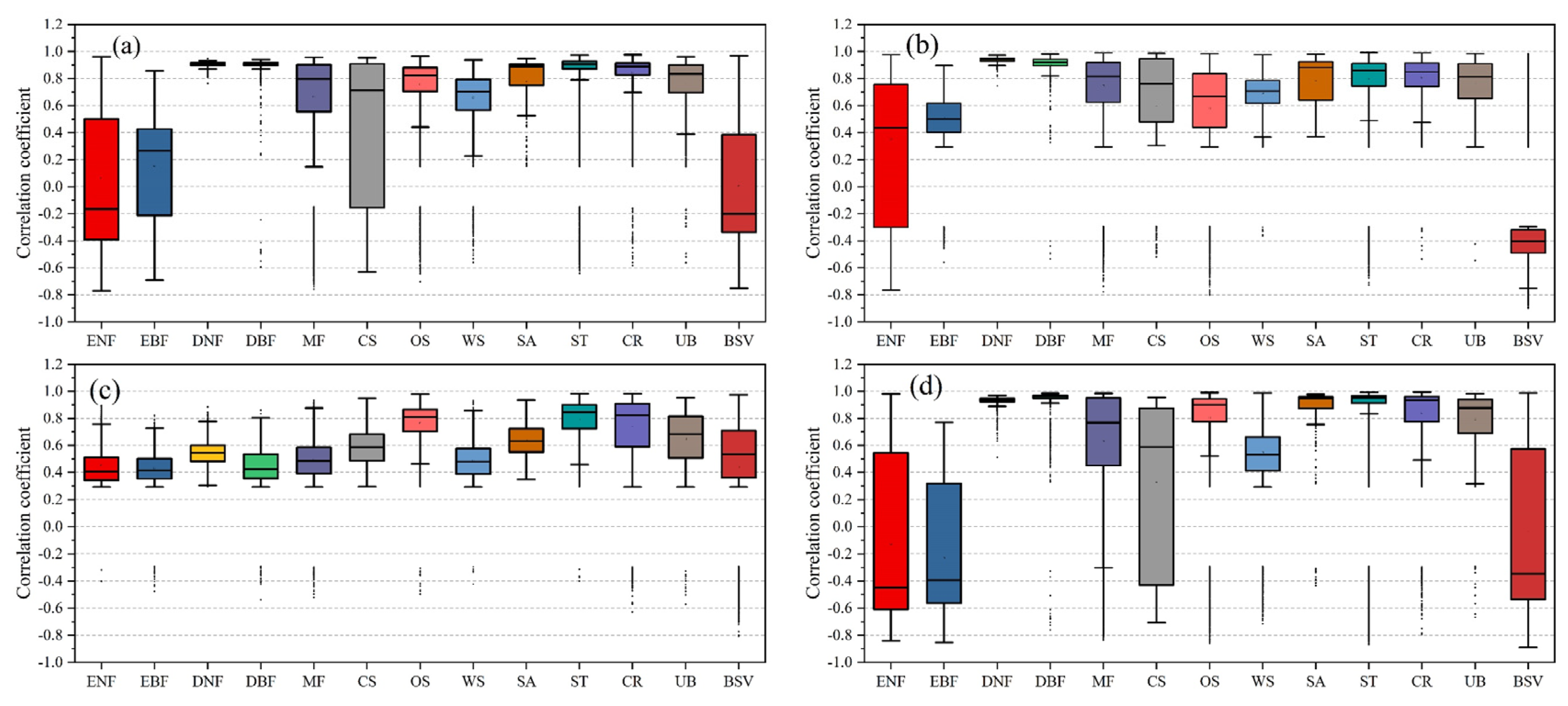
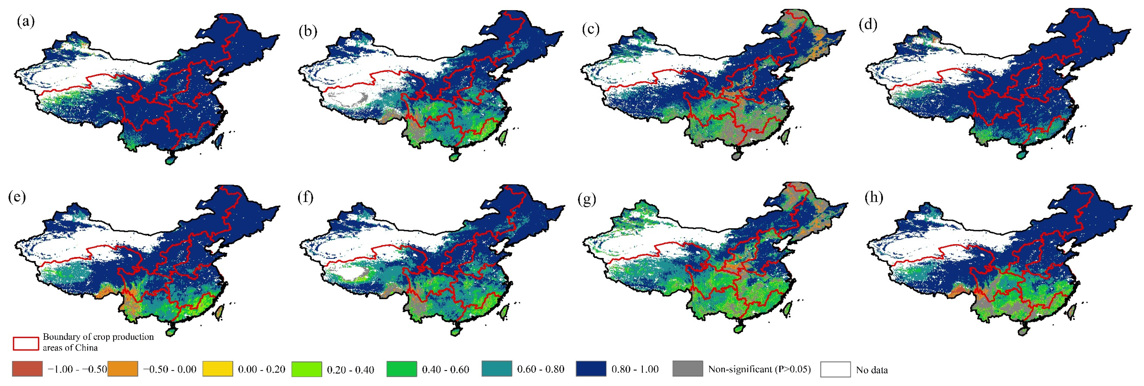
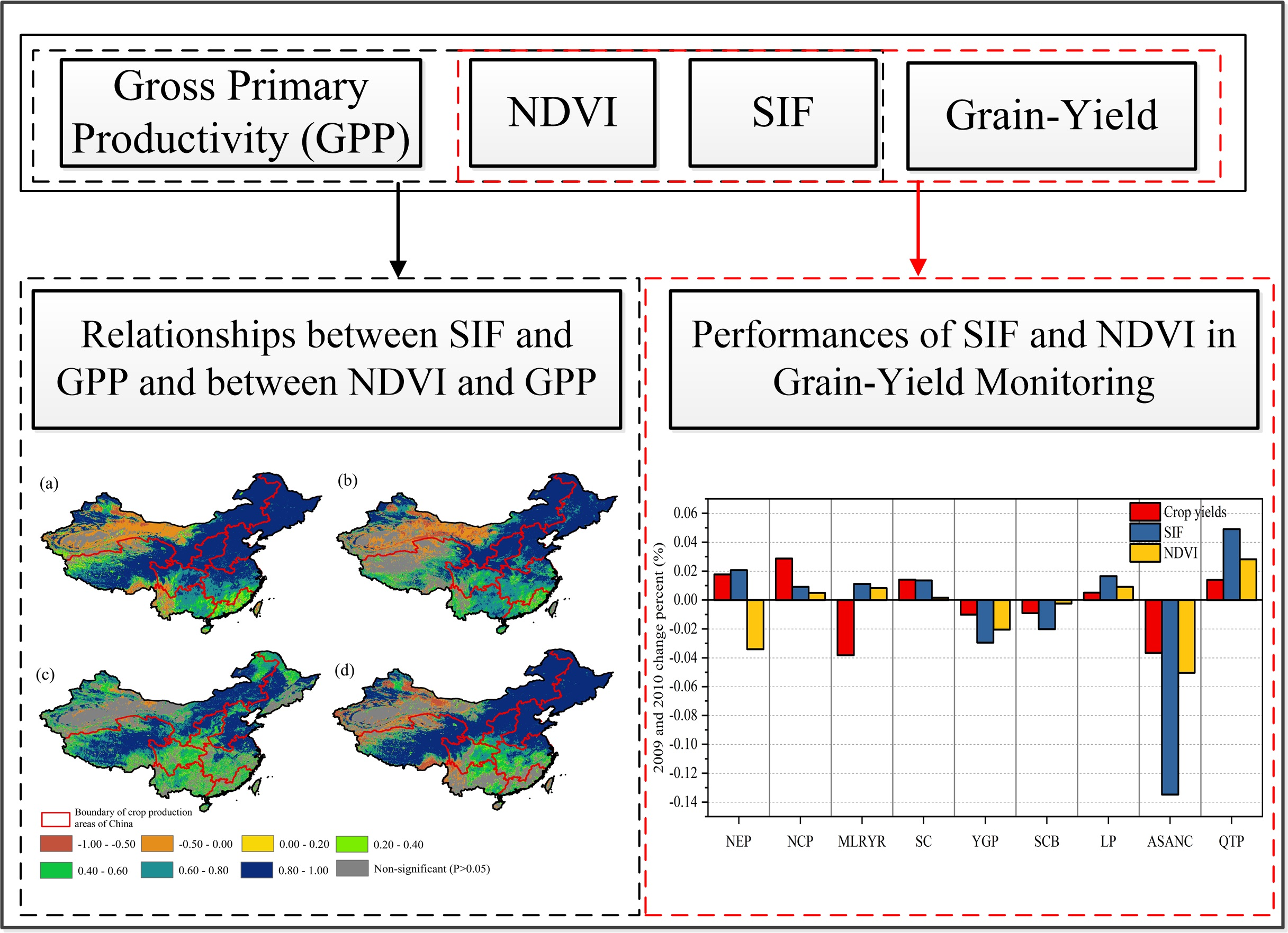
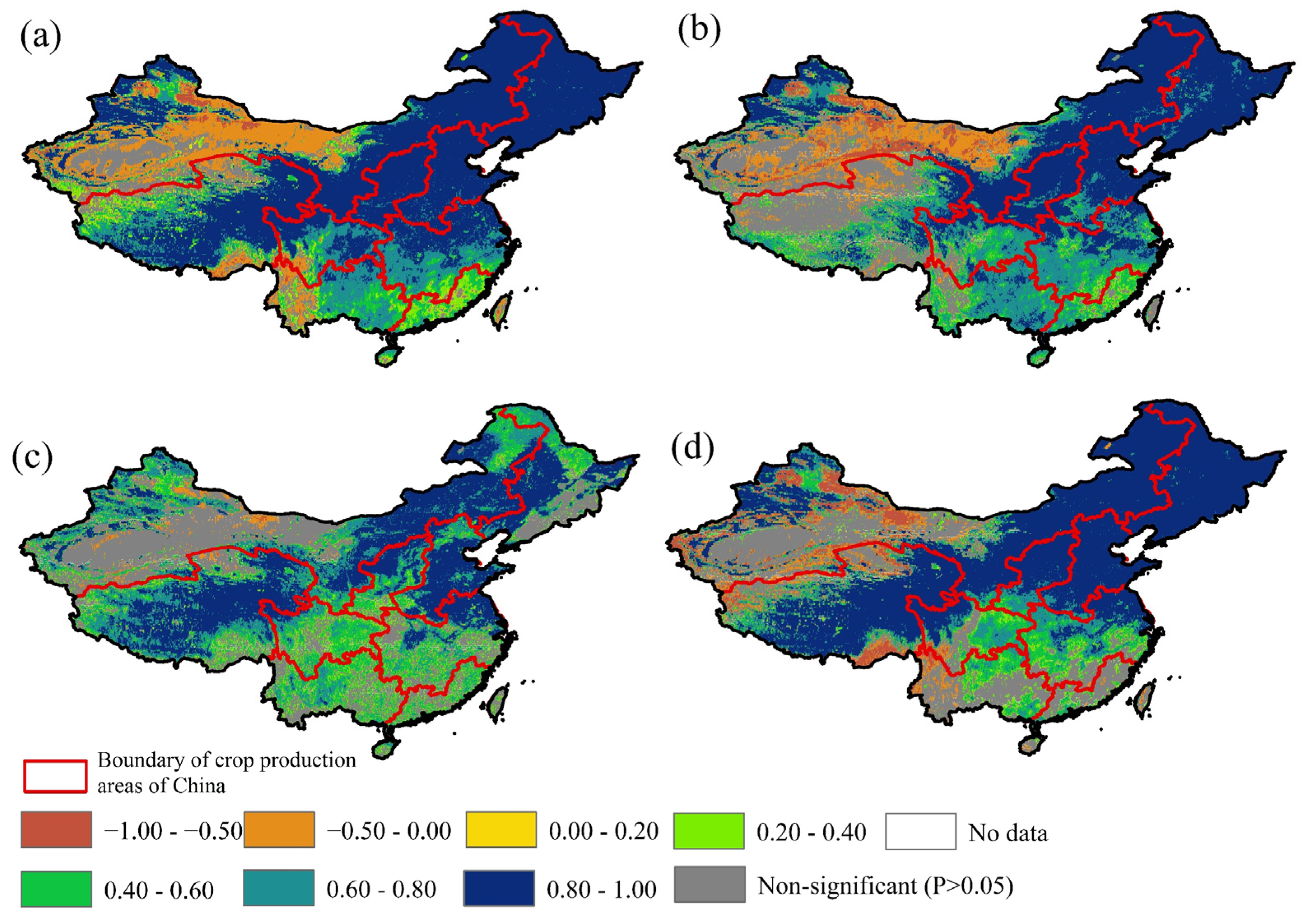
- The spatial distribution characteristics of the relationships between the SIF (NDVI) and the GPP were similar among different seasons, and the correlations were smaller in southern China and northwestern China than in the other regions of China. In general, the correlations between the SIF (NDVI) and the GPP were smaller in the forest vegetation regions during summer than in other seasons. Moreover, the SIF had a stronger correlation with the GPP than the NDVI did in different seasons.
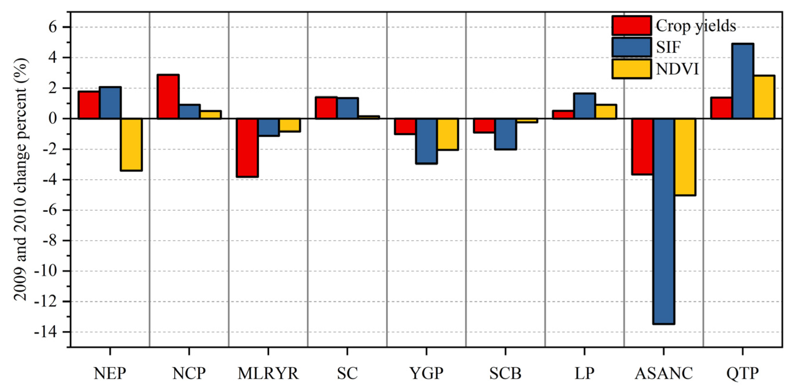
- (3)
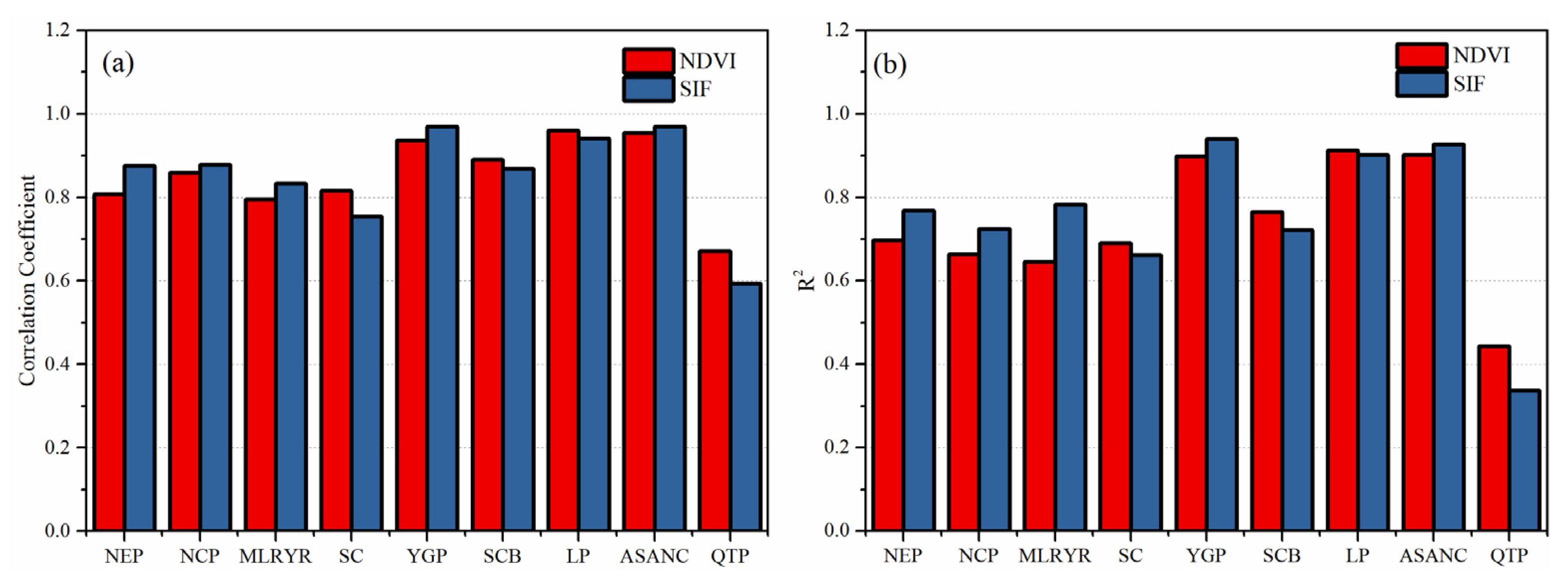
- The PCC and R2 values obtained between the SIF and the per-unit grain yield were generally higher than those obtained between the NDVI and the per-unit grain yield. The percentage changes in the per-unit grain yield and SIF were similar, indicating that the SIF could capture the effect of the drought on the grain yields better than the NDVI could.
Author Contributions
Funding
Data Availability Statement
Conflicts of Interest
References
- Chatterjee, A.; Chatterjee, S.; Smith, B.; Cresswell, J.E.; Basu, P. Predicted thresholds for natural vegetation cover to safeguard pollinator services in agricultural landscapes. Agric. Ecosyst. Environ. 2020, 290, 106785. [Google Scholar] [CrossRef]
- Ciais, P.; Reichstein, M.; Viovy, N.; Granier, A.; Ogée, J.; Allard, V.; Aubinet, M.; Buchmann, N.; Bernhofer, C.; Carrara, A.; et al. Europe-wide reduction in primary productivity caused by the heat and drought in 2003. Nature 2005, 437, 529–533. [Google Scholar] [CrossRef] [PubMed]
- Higgins, S.I.; Scheiter, S. Atmospheric CO2 forces abrupt vegetation shifts locally, but not globally. Nature 2012, 488, 209–212. [Google Scholar] [CrossRef]
- Mohammed, G.H.; Colombo, R.; Middleton, E.M.; Rascher, U.; van der Tol, C.; Nedbal, L.; Goulas, Y.; Pérez-Priego, O.; Damm, A.; Meroni, M.; et al. Remote sensing of solar-induced chlorophyll fluorescence (SIF) in vegetation: 50 years of progress. Remote Sens. Environ. 2019, 231, 111177. [Google Scholar] [CrossRef] [PubMed]
- Zhou, Z.Q.; Ding, Y.B.; Shi, H.Y.; Cai, H.J.; Fu, Q.; Liu, S.N.; Li, T.X. Analysis and prediction of vegetation dynamic changes in China: Past, present and future. Ecol. Indic. 2020, 117, 106642. [Google Scholar] [CrossRef]
- He, L.; Chen, J.M.; Liu, J.; Zheng, T.; Wang, R.; Joiner, J.; Chou, S.; Chen, B.; Liu, Y.; Liu, R.G.; et al. Diverse photosynthetic capacity of global ecosystems mapped by satellite chlorophyll fluorescence measurements. Remote Sens. Environ. 2019, 232, 111344. [Google Scholar] [CrossRef]
- Kern, A.; Barcza, Z.; Marjanovic, H.; Arendas, T.; Fodor, N.; Bonts, P.; Bognar, P.; Lichtenberger, J. Statistical modelling of crop yield in Central Europe using climate data and remote sensing vegetation indices. Agric. For. Meteorol. 2018, 260–261, 300–320. [Google Scholar] [CrossRef]
- Peña-Gallardo, M.; Vicente-Serrano, S.M.; Quiring, S.; Svoboda, M.; Hannaford, J.; Tomas-Burguera, M.; Martín-Hernández, N.; Domínguez-Castro, F.; Kenawy, A.E. Response of crop yield to different time-scales of drought in the United States: Spatio-temporal patterns and climatic and environmental drivers. Agric. For. Meteorol. 2019, 264, 40–55. [Google Scholar] [CrossRef] [Green Version]
- Zhou, J.; Zhang, Z.Q.; Sun, G.; Fang, X.R.; Zha, T.G.; Mcnulty, S.; Chen, J.Q.; Jin, Y.; Noormets, A. Response of ecosystem carbon fluxes to drought events in a poplar plantation in Northern China. For. Ecol. Manag. 2013, 300, 33–42. [Google Scholar] [CrossRef]
- Trabucco, A.; Zomer, R.J.; Bossio, D.A.; van Straaten, O.; Verchot, L.V. Climate change mitigation through afforestation/reforestation: A global analysis of hydrologic impacts with four case studies. Agric. Ecosyst. Environ. 2008, 126, 81–97. [Google Scholar] [CrossRef]
- Jiang, C.; Zhang, H.Y.; Zhang, Z.D.; Wang, D.W. Model-based assessment soil loss by wind and water erosion in China’s Loess Plateau: Dynamic change, conservation effectiveness, and strategies for sustainable restoration. Glob. Planet. Change 2019, 172, 396–413. [Google Scholar] [CrossRef]
- Liu, Y.F.; Liu, Y.; Shi, Z.H.; López-Vicente, M.; Wu, G.L. Effectiveness of re-vegetated forest and grassland on soil erosion control in the semi-arid Loess Plateau. Catena 2020, 195, 104787. [Google Scholar] [CrossRef]
- Ye, W.T.; van Dijk, A.I.J.M.; Huete, A.; Yebra, M. Global trends in vegetation seasonality in the GIMMS NDVI3g and their robustness. Int. J. Appl. Earth Obs. 2021, 94, 102238. [Google Scholar] [CrossRef]
- Li, X.; Xiao, J.F. A Global, 0.05-Degree Product of Solar-Induced Chlorophyll Fluorescence Derived from OCO-2, MODIS, and Reanalysis Data. Remote Sens. 2019, 11, 517. [Google Scholar] [CrossRef] [Green Version]
- Wei, T.F.; Shangguan, D.H.; Yi, S.H.; Ding, Y.J. Characteristics and controls of vegetation and diversity changes monitored with an unmanned aerial vehicle (UAV) in the foreland of the Urumqi Glacier No. 1, Tianshan, China. Sci. Total Environ. 2021, 771, 145433. [Google Scholar] [CrossRef] [PubMed]
- Wan, J.Z.; Wang, C.J.; Qu, H.; Liu, R.; Zhang, Z.X. Vulnerability of forest vegetation to anthropogenic climate change in China. Sci. Total Environ. 2018, 621, 1633–1641. [Google Scholar] [CrossRef]
- Yang, J.L.; Ding, J.W.; Xiao, X.M.; Dai, J.H.; Wu, C.Y.; Xia, J.Y.; Zhao, G.S.; Zhao, M.M.; Li, Z.L.; Zhang, Y.; et al. Divergent shifts in peak photosynthesis timing of temperate and alpine grasslands in China. Remote Sens. Environ. 2019, 233, 111395. [Google Scholar] [CrossRef]
- Liu, F.; Wang, C.K.; Wang, X.C. Sampling protocols of specific leaf area for improving accuracy of the estimation of forest leaf area index. Agric. For. Meteorol. 2021, 298–299, 108286. [Google Scholar] [CrossRef]
- Xu, J.T.; Cai, H.J.; Saddique, Q.; Wang, X.Y.; Li, L.; Ma, C.J.; Liu, Y.J. Evaluation and optimization of border irrigation in different irrigation seasons based on temporal variation of infiltration and roughness. Agric. Water Manag. 2019, 214, 64–77. [Google Scholar] [CrossRef]
- Pinzon, J.; Tucker, C. A Non-Stationary 1981–2012 AVHRR NDVI3g Time Series. Remote Sens. 2014, 6, 6929–6960. [Google Scholar] [CrossRef] [Green Version]
- Chang, C.Y.; Zhou, R.Q.; Kria, O.; Marri, S.; Skovira, J.; Gu, L.H.; Sun, Y. An Unmanned Aerial System (UAS) for concurrent measurements of solar-induced chlorophyll fluorescence and hyperspectral reflectance toward improving crop monitoring. Agric. For. Meteorol. 2020, 294, 108145. [Google Scholar] [CrossRef]
- Fan, X.; Liu, Y. A global study of NDVI difference among moderate-resolution satellite sensors. ISPRS J. Photogramm. 2016, 121, 177–191. [Google Scholar] [CrossRef]
- Pengra, B.; Long, J.; Dahal, D.; Stehman, S.V.; Loveland, T.R. A global reference database from very high resolution commercial satellite data and methodology for application to Landsat derived 30 m continuous field tree cover data. Remote Sens. Environ. 2015, 165, 234–248. [Google Scholar] [CrossRef]
- Shi, H.Y.; Chen, J. Characteristics of climate change and its relationship with land use/cover change in Yunnan Province, China. Int. J. Climatol. 2018, 38, 2520–2537. [Google Scholar] [CrossRef]
- Quiring, S.M.; Ganesh, S. Evaluating the utility of the Vegetation Condition Index (VCI) for monitoring meteorological drought in Texas. Agric. For. Meteorol. 2010, 150, 330–339. [Google Scholar] [CrossRef]
- Bento, V.A.; Gouveia, C.M.; DaCamara, C.C.; Trigo, I.F. A climatological assessment of drought impact on vegetation health index. Agric. For. Meteorol. 2018, 259, 286–295. [Google Scholar] [CrossRef]
- Shammi, S.A.; Meng, Q.M. Use time series NDVI and EVI to develop dynamic crop growth metrics for yield modeling. Ecol. Indic. 2021, 121, 107124. [Google Scholar] [CrossRef]
- Chen, S.; Huang, Y.; Wang, G. Detecting drought-induced GPP spatiotemporal variabilities with sun-induced chlorophyll fluorescence during the 2009/2010 droughts in China. Ecol. Indic. 2021, 121, 107092. [Google Scholar] [CrossRef]
- Ding, Y.B.; Xu, J.T.; Wang, X.W.; Peng, X.B.; Cai, H.J. Spatial and temporal effects of drought on Chinese vegetation under different coverage levels. Sci. Total Environ. 2020, 716, 137166. [Google Scholar] [CrossRef]
- Xu, H.J.; Wang, X.P.; Zhao, C.Y.; Yang, X.M. Diverse responses of vegetation growth to meteorological drought across climate zones and land biomes in northern China from 1981 to 2014. Agric. For. Meteorol. 2018, 262, 1–13. [Google Scholar] [CrossRef]
- Liu, Y.; Dang, C.Y.; Yue, H.; Lyu, C.G.; Dang, X.H. Enhanced drought detection and monitoring using sun-induced chlorophyll fluorescence over Hulun Buir Grassland, China. Sci. Total Environ. 2021, 770, 145271. [Google Scholar] [CrossRef] [PubMed]
- Chen, X.J.; Mo, X.G.; Zhang, Y.C.; Sun, Z.G.; Liu, Y.; Hu, S.; Liu, S.X. Drought detection and assessment with solar-induced chlorophyll fluorescence in summer maize growth period over North China Plain. Ecol. Indic. 2019, 104, 347–356. [Google Scholar] [CrossRef]
- Jeong, S.J.; Schimel, D.; Frankenberg, C.; Drewry, D.T.; Fisher, J.B.; Verma, M.; Berry, J.A.; Lee, J.E.; Joiner, J. Application of satellite solar-induced chlorophyll fluorescence to understanding large-scale variations in vegetation phenology and function over northern high latitude forests. Remote Sens. Environ. 2017, 190, 178–187. [Google Scholar] [CrossRef]
- Wang, F.; Chen, B.Z.; Lin, X.F.; Zhang, H.F. Solar-induced chlorophyll fluorescence as an indicator for determining the end date of the vegetation growing season. Ecol. Indic. 2020, 109, 105755. [Google Scholar] [CrossRef]
- Ding, Y.B.; Xu, J.T.; Wang, X.W.; Cai, H.J.; Zhou, Z.Q.; Sun, Y.N.; Shi, H.Y. Propagation of meteorological to hydrological drought for different climate regions in China. J. Environ. Manag. 2021, 283, 111980. [Google Scholar] [CrossRef]
- Qiu, R.N.; Han, G.; Ma, X.; Xu, H.; Shi, T.Q.; Zhang, M. A comparison of OCO-2 SIF, MODIS GPP, and GOSIF data from Gross Primary Production (GPP) estimation and seasonal cycles in North America. Remote Sens. 2020, 12, 258. [Google Scholar] [CrossRef] [Green Version]
- Li, X.; Xiao, J.F. Global climatic controls on interannual variability of ecosystem productivity: Similarities and differences inferred from solar-induced chlorophyll fluorescence and enhanced vegetation index. Agric. For. Meteorol. 2020, 288–289, 108018. [Google Scholar] [CrossRef]
- Shim, C.; Hong, J.; Hong, J.Y.; Kim, Y.; Kang, M.; Thakuri, B.M.; Kim, Y.; Chun, J. Evaluation of MODIS GPP over a complex ecosystem in East Asia: A case study at Gwangneung flux tower in Korea. Adv. Space Res. 2014, 54, 2296–2308. [Google Scholar] [CrossRef] [Green Version]
- Heinsch, F.A.; Reeves, M.; Votava, P.; Kang, S.; Milesi, C.; Zhao, M.; Glassy, J.; Jolly, W.M.; Kimball, J.S.; Nemannpi, R.R.; et al. User’s Guide GPP and NPP (MOD17A2/A3) Products, NASA MODIS Land Algorithm; MOD17 User’s Guide; University of Montana: Missoula, MT, USA, 2003; pp. 1–57. [Google Scholar]
- Zhao, M.S.; Heinsch, F.A.; Nemani, R.R.; Running, S.W. Improvements of the MODIS terrestrial gross and net primary production global data set. Remote Sens. Environ. 2005, 95, 164–176. [Google Scholar] [CrossRef]
- Wang, S.H.; Zhang, L.F.; Huang, C.P.; Qiao, N. An NDVI-Based Vegetation Phenology Is Improved to be More Consistent with Photosynthesis Dynamics through Applying a Light Use Efficiency Model over Boreal High-Latitude Forests. Remote Sens. 2017, 9, 695. [Google Scholar] [CrossRef] [Green Version]
- Tian, F.; Wu, J.J.; Liu, L.Z.; Leng, S.; Yang, J.H.; Zhao, W.H.; Shen, Q. Exceptional drought across Southeastern Australia caused by extreme lack of precipitation and its impacts on NDVI and SIF in 2018. Remote Sens. 2019, 12, 54. [Google Scholar] [CrossRef] [Green Version]
- Zhou, Z.Q.; Shi, H.Y.; Fu, Q.; Ding, Y.B.; Li, T.X.; Wang, Y.; Liu, S.N. Characteristics of propagation from meteorological drought to hydrological drought in the Pearl River Basin. J. Geophys. Res. Atmos. 2021, 126, e2020JD033959. [Google Scholar] [CrossRef]
- Wang, S.P.; Wang, J.S.; Feng, J.Y. Drought in China and its impact and causes in the autumn of 2010. J. Arid. Meteorol. 2010, 4, 499–504. (In Chinese) [Google Scholar]
- Wang, J.S.; Zhang, Q.; Wang, S.P.; Wang, Y.; Wang, J.; Yao, Y.B.; Ren, Y.L. Characteristic analysis of drought disaster chain in Southwest and South China. J. Arid. Meteorol. 2015, 33, 187–194. [Google Scholar]
- Xu, C.; McDowell, N.G.; Fisher, R.A.; Wei, L.; Sevanto, S.; Chrisrtoffersen, B.O.; Wang, E.S.; Middleton, R.S. Increasing impacts of extreme droughts on vegetation productivity under climate change. Nat. Clim. Chang. 2019, 9, 948–953. [Google Scholar] [CrossRef] [Green Version]
- Wang, G.Q.; Liu, S.M.; Liu, T.X.; Fu, Z.Y.; Yu, J.S.; Xue, B.L. Modelling above-ground biomass based on vegetation indexes: A modified approach for biomass estimation in semi-arid grasslands. Int. J. Remote Sens. 2019, 40, 3835–3854. [Google Scholar] [CrossRef]
- Liu, F.; Qin, Q.M.; Zhan, Z.M. A novel dynamic stretching solution to eliminate saturation effect in NDVI and its application in drought monitoring. Chin. Geogr. Sci. 2012, 22, 683–694. [Google Scholar] [CrossRef]
- Cui, T.X.; Sun, R.; Xiao, Z.Q.; Liang, Z.Y.; Wang, J. Simulating spatially distributed solar-induced chlorophyll fluorescence using a BEPS-SCOPE coupling framework. Agric. For. Meteorol. 2020, 295, 108169. [Google Scholar] [CrossRef]
- Wu, W.; Tang, X.P.; Yang, C.; Guo, N.J.; Liu, H.B. Spatial estimation of monthly mean daily sunshine hours and solar radiation across mainland China. Renew. Energy 2013, 57, 546–553. [Google Scholar] [CrossRef]
- Carlson, T.N.; Ripley, D.A. On the relation between NDVI, fractional vegetation cover, and leaf area index. Remote Sens. Environ. 1997, 62, 241–252. [Google Scholar] [CrossRef]
- Fensholt, R.; Proud, S.R. Evaluation of Earth Observation based global long term vegetation trends—Comparing GIMMS and MODIS global NDVI time series. Remote Sens. Environ. 2012, 119, 131–147. [Google Scholar] [CrossRef]
- Hasegawa, K.; Matsuyama, H.; Tsuzuki, H.; Sweda, T. Improving the estimation of leaf area index by using remotely sensed NDVI with BRDF signatures. Remote Sens. Environ. 2010, 114, 514–519. [Google Scholar] [CrossRef]
- Rokni, K.; Musa, T.A. Normalized difference vegetation change index: A technique for detecting vegetation changes using Landsat imagery. Catena 2019, 178, 59–63. [Google Scholar] [CrossRef]
- Ma, J.; Xiao, X.; Zhang, Y.; Chen, B.; Zhao, B. Spatial-temporal consistency between gross primary productivity and solar-induced chlorophyll fluorescence of vegetation in China during 2007–2014. Sci. Total Environ. 2018, 639, 1241–1253. [Google Scholar] [CrossRef]
- Chang, Q.; Xiao, X.M.; Jiao, W.Z.; Wu, X.C.; Doughty, R.; Wang, J.; Du, L.; Zou, Z.H.; Qin, Y.W. Assessing consistency of spring phenology of snow-covered forests as estimated by vegetation indices, gross primary production, and solar-induced chlorophyll fluorescence. Agric. For. Meteorol. 2019, 275, 305–316. [Google Scholar] [CrossRef]
- Guo, P.P.; Guo, K.J.; Ren, Y.; Shi, Y.; Chang, J.; Tani, A.; Ge, Y. Biogenic volatile organic compound emissions in relation to plant carbon fixation in a subtropical urban–rural complex. Landsc. Urban Plan. 2013, 119, 74–84. [Google Scholar] [CrossRef]
- Xu, J.T.; Cai, H.J.; Wang, X.Y.; Ma, C.G.; Lu, Y.J.; Ding, Y.B.; Wang, X.W.; Chen, H.; Wang, Y.F.; Saddique, Q. Exploring optimal irrigation and nitrogen fertilization in a winter wheat-summer maize rotation system for improving crop yield and reducing water and nitrogen leaching. Agric. Water Manag. 2020, 228, 105904. [Google Scholar] [CrossRef]
- Zhou, Z.Q.; Shi, H.Y.; Fu, Q.; Li, T.X.; Gan, T.Y.; Liu, S.N. Assessing spatiotemporal characteristics of drought and its effects on climate-induced yield of maize in Northeast China. J. Hydrol. 2020, 588, 125097. [Google Scholar] [CrossRef]
- Yang, X.; Tang, J.; Mustard, J.F.; Lee, J.E.; Rossini, M.; Joiner, J.; Munger, J.W.; Kornfeld, A.; Richardson, A.D. Solar-induced chlorophyll fluorescence that correlates with canopy photosynthesis on diurnal and seasonal scales in a temperate deciduous forest. Geophys. Res. Lett. 2015, 42, 2977–2987. [Google Scholar] [CrossRef]


| Vegetation Type | Abbreviation | |
|---|---|---|
| Class 1 | Class 2 | |
| Forest (17.85%) | Evergreen needleleaf forest (3.22%) | ENF |
| Evergreen broadleaf forest (12.43%) | EBF | |
| Deciduous needleleaf forest (1.20%) | DNF | |
| Deciduous broadleaf forest (2.04%) | DBF | |
| Mixed forest (81.11%) | MF | |
| Shrubland (10.21%) | Closed shrublands (0.69%) | CS |
| Open shrublands (99.31%) | OS | |
| Grassland (24.05%) | Woody savannas (14.51%) | WS |
| Savannas (0.24%) | SA | |
| Steppes (85.25%) | ST | |
| Croplands (23.28%) | CR | |
| Urban and built-up areas (0.81%) | UB | |
| Barren or sparsely vegetated areas (23.80%) | BSV | |
Publisher’s Note: MDPI stays neutral with regard to jurisdictional claims in published maps and institutional affiliations. |
© 2022 by the authors. Licensee MDPI, Basel, Switzerland. This article is an open access article distributed under the terms and conditions of the Creative Commons Attribution (CC BY) license (https://creativecommons.org/licenses/by/4.0/).
Share and Cite
Zhou, Z.; Ding, Y.; Liu, S.; Wang, Y.; Fu, Q.; Shi, H. Estimating the Applicability of NDVI and SIF to Gross Primary Productivity and Grain-Yield Monitoring in China. Remote Sens. 2022, 14, 3237. https://doi.org/10.3390/rs14133237
Zhou Z, Ding Y, Liu S, Wang Y, Fu Q, Shi H. Estimating the Applicability of NDVI and SIF to Gross Primary Productivity and Grain-Yield Monitoring in China. Remote Sensing. 2022; 14(13):3237. https://doi.org/10.3390/rs14133237
Chicago/Turabian StyleZhou, Zhaoqiang, Yibo Ding, Suning Liu, Yao Wang, Qiang Fu, and Haiyun Shi. 2022. "Estimating the Applicability of NDVI and SIF to Gross Primary Productivity and Grain-Yield Monitoring in China" Remote Sensing 14, no. 13: 3237. https://doi.org/10.3390/rs14133237
APA StyleZhou, Z., Ding, Y., Liu, S., Wang, Y., Fu, Q., & Shi, H. (2022). Estimating the Applicability of NDVI and SIF to Gross Primary Productivity and Grain-Yield Monitoring in China. Remote Sensing, 14(13), 3237. https://doi.org/10.3390/rs14133237