Technical Note

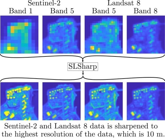
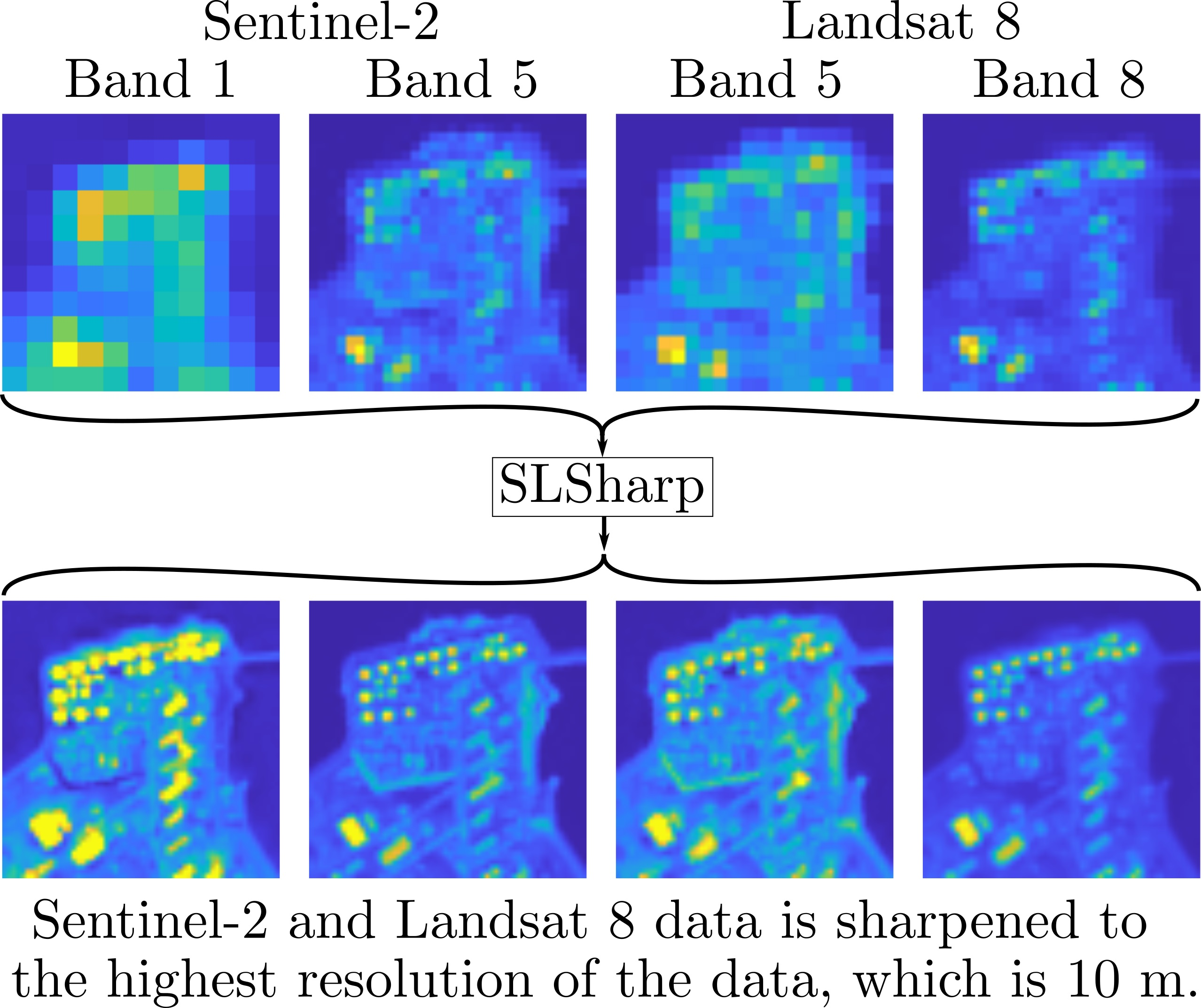
Fusing Sentinel-2 and Landsat 8 Satellite Images Using a Model-Based Method

by
Jakob Sigurdsson
*,
Sveinn E. Armannsson
,
Magnus O. Ulfarsson
and
Johannes R. Sveinsson
Faculty of Electrical and Computer Engineering, University of Iceland, Hjardarhagi 2-6, 107 Reykjavik, Iceland
*
Author to whom correspondence should be addressed.
Remote Sens. 2022, 14(13), 3224; https://doi.org/10.3390/rs14133224
Submission received: 31 May 2022 / Revised: 30 June 2022 / Accepted: 30 June 2022 / Published: 5 July 2022
(This article belongs to the Special Issue Advanced Super-resolution Methods in Remote Sensing)

Abstract

:
The Copernicus Sentinel-2 (S2) constellation comprises of two satellites in a sun-synchronous orbit. The S2 sensors have three spatial resolutions: 10, 20, and 60 m. The Landsat 8 (L8) satellite has sensors that provide seasonal coverage at spatial resolutions of 15, 30, and 60 m. Many remote sensing applications require the spatial resolutions of all data to be at the highest resolution possible, i.e., 10 m for S2. To address this demand, researchers have proposed various methods that exploit the spectral and spatial correlations within multispectral data to sharpen the S2 bands to 10 m. In this study, we combined S2 and L8 data. An S2 sharpening method called Sentinel-2 Sharpening (S2Sharp) was modified to include the 30 m and 15 m spectral bands from L8 and to sharpen all bands (S2 and L8) to the highest resolution of the data, which was 10 m. The method was evaluated using both real and simulated data.

Graphical Abstract

1. Introduction

In 2013, the Landsat 8 satellite was launched, equipped with an Operational Land Imager (OLI) and thermal infrared (TIR) sensors. The L8 OLI provides seven spectral bands at a 30 m spatial resolution and one panchromatic band at a 15 m resolution. The revisit rate of the L8 is 16 days and, along with the fact that the area being imaged by the L8 often has cloud coverage, this means that time-series L8 data are often very sparse. In 2015 and 2017, the European Space Agency launched the Sentinel-2A and 2B satellites, respectively. The S2 multispectral imager (MSI) provides thirteen spectral bands: four bands at a spatial resolution of 10 m, six bands at 20 m, and three bands at 60 m.
In Figure 1 [1], the wavelengths and placements of the S2 MSI bands and the L8 OLI bands are shown. The spatial resolution of the S2 bands is higher (10 m or 20 m) than the resolution of the corresponding L8 bands (30 m). The facts that the S2 and L8 cover similar wavelengths and the data from both of these satellites share the same geographic coordinate system make them excellent candidates for data fusion. Many remote sensing applications require all data that are used to be at the same resolution. To address this requirement, considerable effort has been put into the subject of super-resolving S2 bands so that they all have a 10 m spatial resolution [2,3,4,5,6,7,8,9,10,11].
Together, the S2-A and S2-B satellites provide a revisit rate of 5 days [12] worldwide. This high revisit rate makes S2 data very useful for many applications, such as environmental monitoring and risk and disaster mapping.
Within the remote sensing community, there has been a long history of data fusion [13,14,15,16,17,18,19,20,21]. This is an important remote sensing topic and with the rapid development of remote sensing technologies and sensors, the importance of image fusion techniques has only increased. The need for methods that are capable of making use of data that were acquired from different sensors is very important and beneficial as they could facilitate new research and improve results. The wide coverage and frequent revisit rate of the S2 make it a good candidate for data fusion [22,23,24]. In [25], 5-day L8 OLI and harmonized surface reflectance data from the S2 MSI were combined and resampled to a 30 m resolution using the S2 tiling system.
In [26,27], S2 and Sentinel-1 (S1) data were combined. In [28], the comparative performance of decision- and pixel-level data fusion ensemble classifier maps using S2, L8, and Landsat 7 data was evaluated. A self-supervised framework for SAR–optical data fusion and land cover mapping tasks was also proposed, in which SAR and optical images were fused using a multiview contrastive loss at the image level and super-pixel level. In [29], the 10 m and 20 m S2 reflectance bands were sharpened using the 3 m Planetscope reflectance bands, providing a potential method for improved global monitoring. In the study, two well-established and computationally efficient sharpening methods were used. Additionally, both of the spectrally non-overlapping bands between the two sensors and the surface changes that could occur between acquisitions were examined. In [30], a methodological approach to fusing S2 and S1 data for the land cover mapping of the Lower Magdalena region in Colombia was proposed. First, the SEN2COR toolbox from ESA was used to preprocess the data, followed by land cover–land use classification using support vector machines. In [31], numerical regression was used to fuse spectral indices, based on high-resolution images from an unpiloted aerial vehicle and S2 images. In [32], an attentional super-resolution convolutional neural network was used to fuse S2 and L8 data to create a 10 m resolution NDVI (normalized difference vegetation index) time series, which it was evaluated using two heterogeneous areas. Inspired by deep learning, an extended super-resolution convolutional neural network framework was also developed in [33] to fuse S2 and L8 images.
The main contribution of this paper is the proposal of a method that jointly sharpens both S2 and L8 data to a resolution of 10 m. The method was developed by extending the S2Sharp (https://github.com/mou12/S2Sharp, accessed on 10 January 2022) method, which was proposed in [7]. Other contributions of this paper include the estimation process of the point spread function for L8 data, which is needed for the proposed method, and the way in which the 15 m L8 panchromatic band is used in the sharpening process.

2. The Method

The method for sharpening S2 data, that was presented in [7] (S2Sharp), was modified to sharpen both S2 and L8 data. S2Sharp sharpens both the 20 m and 60 m S2 bands to a spatial resolution of 10 m. The method belongs to a family of variational approaches that assume that multiresolution acquisitions can be represented using a linear acquisition model.
The method uses projections onto a low-dimensional subspace that are automatically estimated in the optimization process. The minimization problem that S2 solves is non-convex and cyclic descent is used for the optimization. The cost function that S2Sharp minimizes is:
J ( U , Z ) = i = 1 L S 2 1 2 y i M i B i Z u ( i ) 2 + j = 1 p λ j ϕ w z j ,
where L S 2 is the number of channels ( L S 2 = 12 , i.e., all S2 bands except for band number 10), y i is the (vectorized) S2 image observed at band i, Z u ( i ) is an estimate of the full-resolution images at band i, M i is a downsampling operator, B i is a blurring operator (according to the S2 sensor specifications), Z is an n × p full-rank matrix ( p < L S 2 < < n ), U = [ u ( i ) T ] i = 1 L S 2 is an L S 2 × p orthonormal matrix that spans a p-dimensional subspace in R L × 1 , and n is the number of pixels in the highest resolution bands. The regularization term ϕ w is a spatial regularization term, which is controlled by the tuning parameters λ j .
To be able to sharpen both S2 and L8 data, we introduced a new method called Sentinel-2 Landsat 8 Sharpening (SLSharp), which was based on S2Sharp. To accomplish this, the following needs had to be addressed:
(1)
The cost function used by S2Sharp (1) needed to be modified to include the L8 bands;
(2)
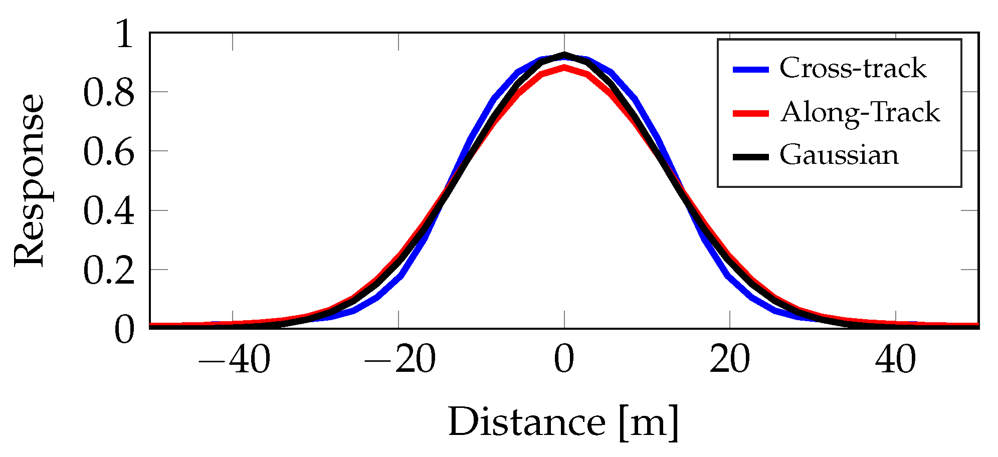
The point spread function (PSF) of the L8 data needed to be estimated;
(3)
The 15 m panchromatic band of the L8 data needed to be resampled.
The first task was to modify the S2Sharp cost function (1) in the following way:
J m ( U , Z ) = i = 1 L 1 2 y i M i B i Z u ( i ) 2 + j = 1 p λ j ϕ w z j ,
where L = L S 2 + 8 = 20 and y i , i > 12 are the L8 OLI bands. This extension of S2Sharp was similar to the extension that was carried out in [21], but it was not as straightforward. The second task was to estimate the PSF of each L8 band. S2Sharp assumes that the PSF is a symmetrical 2D Gaussian function and relies on the variance of the Gaussian function. For the S2 data, the variance is calculated [4] using a calibrated modulation transfer function (MTF), which is supplied by the S2 technical guide [34] for each band. The L8 OLI spatial response for each band is represented in terms of two separable along- and across-track line spread functions [35]. To estimate the PSF for the L8 data, the same assumption was made as for the S2 data, i.e., that the PSF was a symmetrical 2D Gaussian function. The average spatial response for each band was calculated by averaging the along- and across-track OLI spatial responses; then, the variance of the Gaussian function was found using a least squares estimation. In Figure 2, the OLI spatial response for band number 6 is shown, along with the estimated Gaussian function. The spatial response functions for the other L8 bands were similar.
Another issue with sharpening the L8 images was that the SLSharp method was only able to sharpen bands that had a spatial resolution that was an integer multiple of 10 m. The panchromatic band of the L8 data had a spatial resolution of 15 m, which is not an integer multiple of 10 m. The third task was to solve this issue. We downsampled this band using bicubic interpolation to a 20 m spatial resolution and then the method was able to sharpen the band to 10 m. This was not optimal as the downsampling operation threw out some information from the panchromatic band. To alleviate this issue, we also upsampled the panchromatic band using bicubic interpolation to achieve a resolution of 10 m. By doing these upsampling and downsampling operations, the method could sharpen the 15 m panchromatic band of the L8 data without discarding any information. The downside to this approach was that two bands with 10 m and 20 m resolutions were used instead of one 15 m panchromatic band, which slightly increased the required computations.

3. Evaluation

To evaluate SLSharp qualitatively, we used S2 and L8 images of southwest Iceland. Both images were acquired on 7 July 2019. The S2 image was acquired at 13:14 UTC and the L8 image was acquired at 12:46 UTC. A 288 × 288 pixel crop of the whole image was used. We also used S2 and L8 images of Glen Canyon Dam and its surroundings in Arizona, USA. The S2 image was acquired on 12 December 2021 at 18:24 UTC and the L8 image was acquired on 1 December 2021 at 18:03 UTC. A 540 × 540 pixel crop from the whole image was used. We refer to the images from Iceland and Arizona as IS and AZ images, respectively. These two sets of images were chosen because they were cloud-free, contained interesting details, and were heterogeneous. In Figure 3, the RGB images that were generated using bands 2–4 of the S2 and L8 images are shown.
The S2 RGB images were much sharper since the spatial resolution of bands 2–4 was 10 m compared to the 30 m resolution of the L8 bands. The regions of interest (ROIs) are within the yellow rectangles. Within the IS ROI is an urban area with clearly visible houses and a shoreline. Within the AZ ROI, the Glen Canyon Dam is clearly visible. To obtain the best results from SLSharp, a number of tuning parameters needed to be estimated and to do so, the method proposed in [36,37] was used. The parameters that needed to be estimated were p, the rank of the subspace, and the spatial regularization parameters λ j and j = 1 , , p .
The results obtained using SLSharp were compared to a modified version of SupReME, which is the S2 sharpening method presented in [4]. SupReME makes the same assumption as SLSharp, i.e., the PSF is a uniform 2D Gaussian function, so the variance in the L8 spectral response that was described in Section 2 could also be used to modify SupReME so that it was able to sharpen the L8 data. This modified version of SupReME, denoted here as the baseline method, served as a baseline for the performance of SLSharp. The results were also compared to the area-to-point regression kriging (ATPRK) [38] fusion method. The ATPRK fusion method was implemented by the authors of this paper as described in [38], using the code from the GitHub page of the ATPRK authors [39]. Figure 4 and Figure 5 show the sharpened results of the IS and AZ ROIs, respectively (S2 bands 2, 5, and 7; L8 bands 1, 5, and 8).
By examining the results within the ROI in Figure 4 and Figure 5, it could be seen that SLSharp outperformed the ATPRK and baseline methods in all bands. The images that were obtained using SLSharp had more detail and the outlines of the buildings were crisper and had fewer artifacts.
A quantitative evaluation of the relative dimensionless global error (ERGAS), root mean square error (RMSE), spectral angle mapper (SAM) in degrees, signal-to-reconstruction error (SRE) in dB, structural similarity index measure (SSIM), and universal image quality index (UIQI) metrics was performed using the same images at reduced scales, with Wald’s protocol for the IS and AZ images as well as a synthesized image of Escondido [40,41,42]. The images were first reduced by 2× and 6×. Bayesian optimization was then used to find the set of parameters that yielded the best results when resolving the 20 m and 60 m bands back to their original resolution. These parameters were then used to super-resolve the original full-scale images.
The Escondido image was simulated from a fine resolution AVIRIS image using methods that were similar to those in [7,8]. The original AVIRIS image of an area near San Diego, CA, USA, was acquired in November 2011. The image was 790 × 6796 pixels in 224 bands that spanned a spectral range of 366–2496 nm and covered the range of the S2 and L8 OLI sensors.
Reduced resolution versions of all bands were generated at 2× pixel size, 3× pixel size, and 6× pixel size. This was carried out by applying appropriate filters to simulate the PSF of each S2 and L8 OLI band before downgrading them by a factor of 2, 3, and 6, respectively.
The S2 and L8 versions were simulated by applying the S2 and L8 OLI spectral responses to a patch of the AVIRIS data, which depicted parts of the city of Escondido and its suburbs. Twenty bands at a spatial resolution of 5 m were filtered, subsampled and cropped to yield a 288 × 288 pixel ground truth for each band at a 10 m resolution. The bands were then filtered using the estimated Gaussian PSF of the S2 and L8 sensors and downgraded to yield four bands at a 10 m resolution, a single band at a 15 m resolution, six bands at a 20 m resolution, seven bands at a 30 m resolution, and two bands at a 60 m resolution. The 15 m panchromatic band of the L8 data was then upsampled and downsampled to a 10 m and 20 m resolution, as before, for use with SLSharp. For comparison, the baseline and ATPRK methods were also evaluated using the same data.
SLSharp performed better, in terms of sharpening most of the bands of the reduced scale images, in all metrics apart from UIQI, for which ATPRK had a slight advantage in the S2 bands and bands L1 and L7. However, the average UIQI that was obtained using SLSharp was lower. The simulated Escondido image results were more band-dependent. By examining the Escondido results in Table 1 and Table 2, the following was noted:
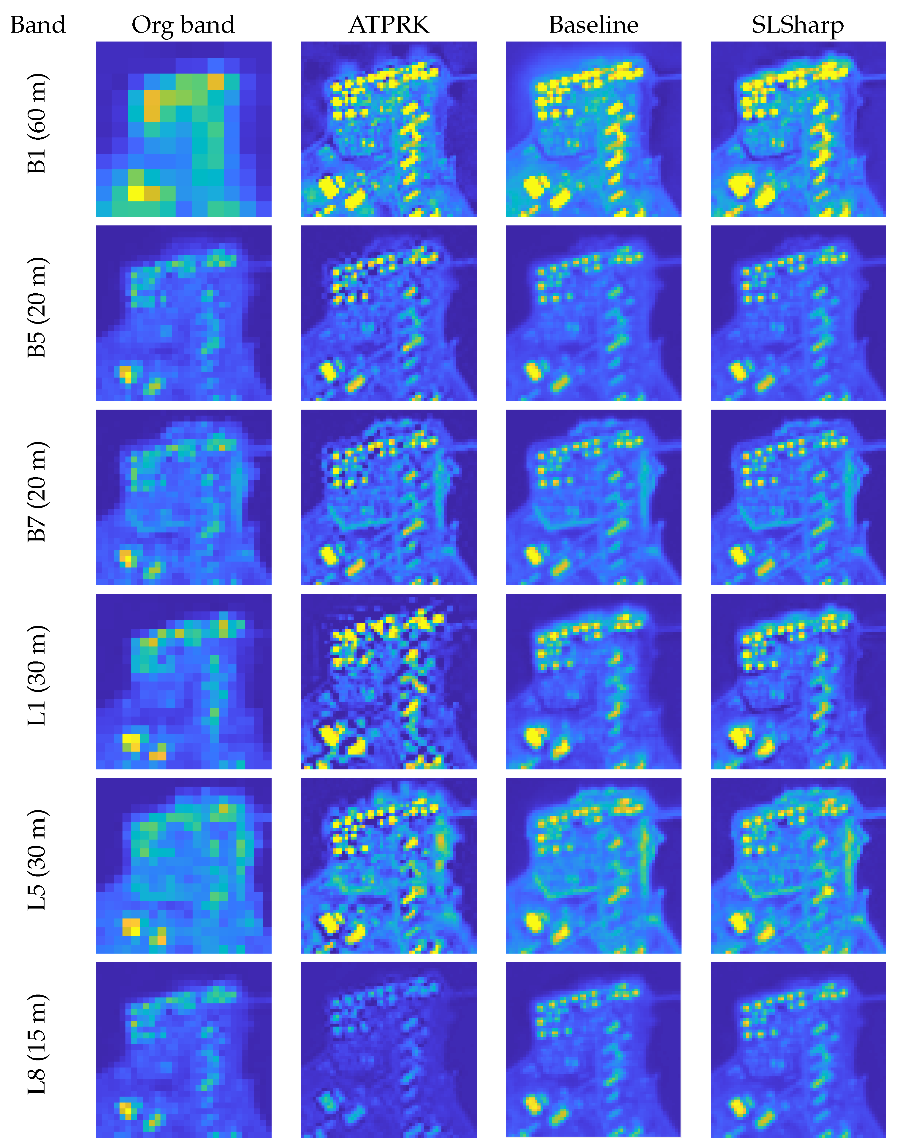
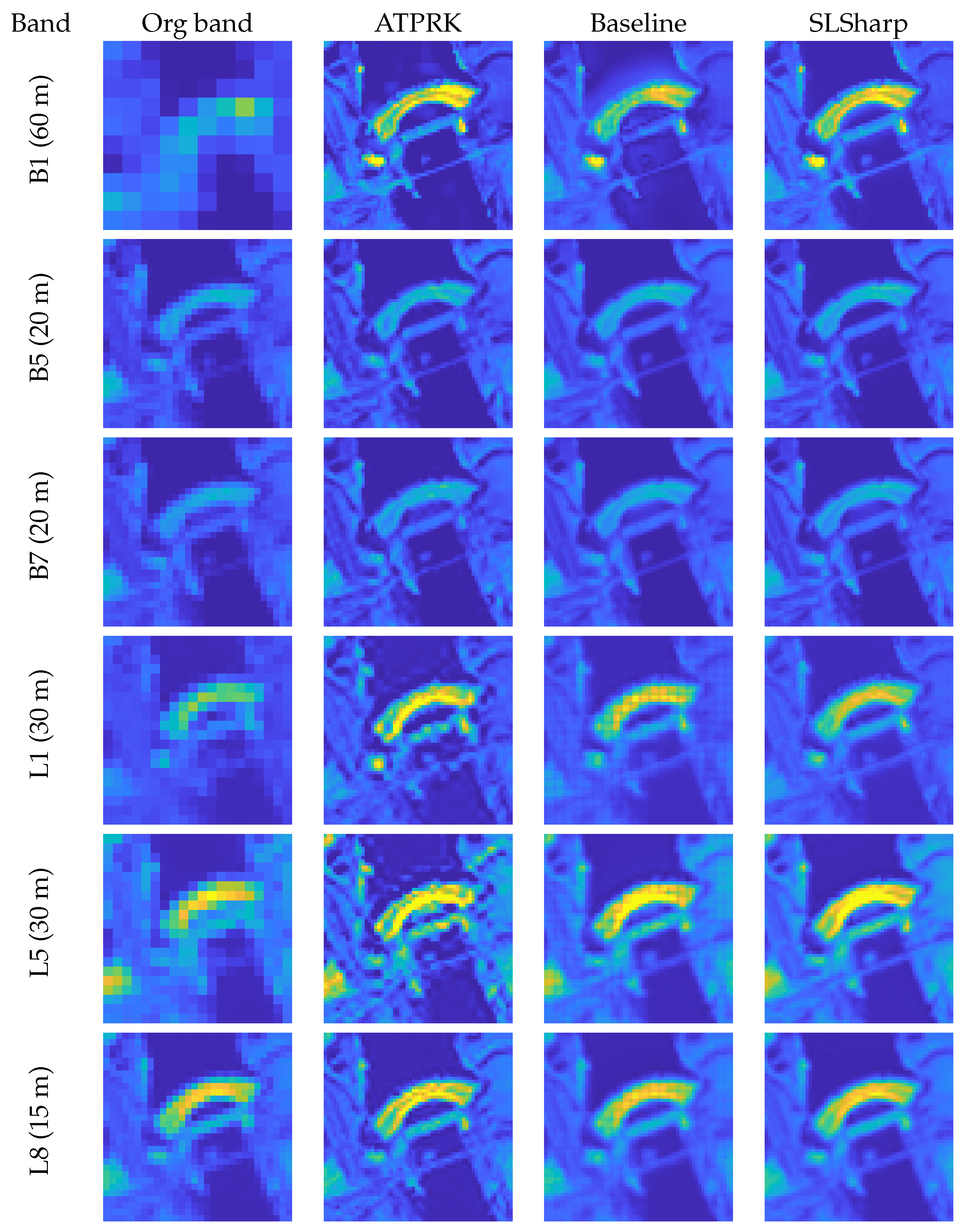
  • The ATPRK method obtained better SRE, SSIM, and UIQI scores in the simulated NIR bands B11, B12, L6, and L7;
  • The baseline method obtained better SRE, SSIM, and UIQI scores in the simulated 60 m bands B1 and B9;
  • Although SLSharp performed the best in most of the simulated bands, the baseline method obtained the best ERGAS, SRE, and SSIM scores and the ATPRK method obtained a better UIQI score when averaged across all bands.
Although the results were generated using equivalent procedures, there were significant differences between the performances for the reduced scale images and the simulated image. All methods had better average scores when using the simulated image.
SLSharp was tuned to maximize the average SRE across all bands. Evidently, this did not necessarily maximize all of the other unrelated metrics or the SRE scores of individual bands. The differences between the baseline method and SLSharp for a few isolated bands in the AZ and IS images were negligible, apart from SAM, which is a measure of spectral quality and would not be reflected in the visual quality of each band when viewed spatially.
The evaluated metrics for which the baseline method achieved better scores (ERGAS, SRE, and SSIM) were not measures of perceptual image quality but rather of distortion, which has long been known to be an unreliable indicator of perceptual image quality [41,43]. This could be confirmed by comparing the 30 m L8 bands in Figure 4 and Figure 5, which look much better when processed with SLSharp than the baseline method but have identical RMSE scores, as shown in Table 1. For SSIM, the differences were very small for the bands for which the baseline method performed better (a single band (L6) showed a 0.02 difference, whereas the others were 0.01 or less), while SLSharp outperformed the baseline method in the other bands by up to 0.05.

4. Conclusions

In this paper, we proposed the S2 L8 Sharpening (SLSharp) method to fuse Landsat 8 and Sentinel-2 satellite data. The S2Sharp algorithm was modified to include the 30 m bands of the L8 OLI, as well as the 15 m panchromatic image. The method was used to sharpen all Landsat 8 OLI and Sentinel-2 bands to a 10 m resolution. The method was evaluated visually, using real images, and quantitatively, using reduced scale and simulated images. Using these data, it was shown that SLSharp could improve the results compared to the baseline and ATPRK methods.

Author Contributions

Original draft prepared by J.S. Writing, reviewing and editing was performed by J.S., S.E.A., M.O.U. and J.R.S. Programming and testing was carried out by J.S. and S.E.A. All authors have read and agreed to the published version of the manuscript.

Funding

This research was funded in part by the Icelandic Research Fund (grant number: 207233-051) and in part by the University of Iceland Research Fund.

Data Availability Statement

All data used in this study were Sentinel-2 data that are available at the ESA Sentinel-2 data hub and Landast 8 data that are available on the USGS Earth Explorer site. The proposed method and the data used in this paper are available at https://github.com/JakobSig/S2L8sharpening.

Conflicts of Interest

The authors declare no conflict of interest. The funders had no role in the design of the study; in the collection, analyses, or interpretation of data; in the writing of the manuscript, or in the decision to publish the results.

Abbreviations

The following abbreviations are used in this manuscript:
2DTwo-dimensional
ATPRKArea-to-Point Regression Kriging
AZArizona
ERGASRelative Dimensionless Global Error
ISIceland
L8Landsat 8
MSIMultispectral Imager
MTFModulation Transfer Function
OLIOperational Land Imager
PSFPoint Spread Function
RMSERoot Mean Square Error
ROIRegion of Interest
S1Sentinel-1
S2Sentinel-2
S2SharpSentinel-2 Sharpening
SAMSpectral Angle Mapper
SLSharpSentinel-2 Landsat 8 Sharpening
SRESignal-to-Reconstruction Error
SSIMStructural Similarity Index Measure
UAVUnpiloted Aerial Vehicle
UIQIUniversal Image Quality Index

References

  1. USGS EROS Archive—Sentinel-2—Comparison of Sentinel-2 and Landsat. Available online: https://www.usgs.gov/centers/eros/science/usgs-eros-archive-sentinel-2-comparison-sentinel-2-and-landsat. (accessed on 25 January 2022).
  2. Wang, Q.; Shi, W.; Li, Z.; Atkinson, P.M. Fusion of Sentinel-2 Images. Remote Sens. Environ. 2016, 187, 241–252. [Google Scholar] [CrossRef] [Green Version]
  3. Brodu, N. Super-Resolving Multiresolution Images With Band-Independent Geometry of Multispectral Pixels. IEEE Trans. Geosci. Remote Sens. 2017, 55, 4610–4617. [Google Scholar] [CrossRef] [Green Version]
  4. Lanaras, C.; Bioucas-Dias, J.; Baltsavias, E.; Schindler, K. Super-Resolution of Multispectral Multiresolution Images from a Single Sensor. In Proceedings of the 2017 IEEE Conference on Computer Vision and Pattern Recognition Workshops (CVPRW), Honolulu, HI, USA, 21–26 July 2017; pp. 1505–1513. [Google Scholar]
  5. Lanaras, C.; Bioucas-Dias, J.M.; Galliani, S.; Baltsavias, E.; Schindler, K. Super-Resolution of Sentinel-2 Images: Learning a Globally Applicable Deep Neural Network. ISPRS J. Photogramm. Remote Sens. 2018, 146, 305–319. [Google Scholar] [CrossRef] [Green Version]
  6. Palsson, F.; Sveinsson, J.R.; Ulfarsson, M.O. Sentinel-2 Image Fusion Using a Deep Residual Network. Remote Sens. 2018, 10, 1290. [Google Scholar] [CrossRef] [Green Version]
  7. Ulfarsson, M.O.; Palsson, F.; Dalla Mura, M.; Sveinsson, J.R. Sentinel-2 Sharpening Using a Reduced-Rank Method. IEEE Trans. Geosci. Remote Sens. 2019, 57, 6408–6420. [Google Scholar] [CrossRef]
  8. Paris, C.; Bioucas-Dias, J.; Bruzzone, L. A Novel Sharpening Approach for Superresolving Multiresolution Optical Images. IEEE Trans. Geosci. Remote Sens. 2019, 57, 1545–1560. [Google Scholar] [CrossRef]
  9. Lin, C.H.; Bioucas-Dias, J.M. An Explicit and Scene-Adapted Definition of Convex Self-Similarity Prior With Application to Unsupervised Sentinel-2 Super-Resolution. IEEE Trans. Geosci. Remote Sens. 2020, 58, 3352–3365. [Google Scholar] [CrossRef]
  10. Nguyen, H.V.; Ulfarsson, M.O.; Sveinsson, J.R.; Sigurdsson, J. Zero-Shot Sentinel-2 Sharpening Using a Symmetric Skipped Connection Convolutional Neural Network. In Proceedings of the IEEE International Geoscience and Remote Sensing Symposium (IGARSS), Waikoloa, HI, USA, 26 September–2 October 2020. [Google Scholar]
  11. Nguyen, H.V.; Ulfarsson, M.O.; Sveinsson, J.R.; Mura, M.D. Sentinel-2 Sharpening Using a Single Unsupervised Convolutional Neural Network With MTF-Based Degradation Model. IEEE J. Sel. Top. Appl. Earth Obs. Remote Sens. 2021, 14, 6882–6896. [Google Scholar] [CrossRef]
  12. Sentinel-2s Observation Scenario. Available online: https://sentinels.copernicus.eu/web/success-stories/-/sentinel-2-s-observation-scenario (accessed on 21 June 2022).
  13. Nunez, J.; Otazu, X.; Fors, O.; Prades, A.; Pala, V.; Arbiol, R. Multiresolution-based image fusion with additive wavelet decomposition. IEEE Trans. Geosci. Remote Sens. 1999, 37, 1204–1211. [Google Scholar] [CrossRef] [Green Version]
  14. Aiazzi, B.; Alparone, L.; Baronti, S.; Garzelli, A. Context-driven fusion of high spatial and spectral resolution images based on oversampled multiresolution analysis. IEEE Trans. Geosci. Remote Sens. 2002, 40, 2300–2312. [Google Scholar] [CrossRef]
  15. Gao, F.; Masek, J.; Schwaller, M.; Hall, F. On the blending of the Landsat and MODIS surface reflectance: Predicting daily Landsat surface reflectance. IEEE Trans. Geosci. Remote Sens. 2006, 44, 2207–2218. [Google Scholar] [CrossRef]
  16. Wang, Z.; Ziou, D.; Armenakis, C.; Li, D.; Li, Q. A comparative analysis of image fusion methods. IEEE Trans. Geosci. Remote Sens. 2005, 43, 1391–1402. [Google Scholar] [CrossRef]
  17. Dalponte, M.; Bruzzone, L.; Gianelle, D. Fusion of Hyperspectral and LIDAR Remote Sensing Data for Classification of Complex Forest Areas. IEEE Trans. Geosci. Remote Sens. 2008, 46, 1416–1427. [Google Scholar] [CrossRef] [Green Version]
  18. Thomas, C.; Ranchin, T.; Wald, L.; Chanussot, J. Synthesis of Multispectral Images to High Spatial Resolution: A Critical Review of Fusion Methods Based on Remote Sensing Physics. IEEE Trans. Geosci. Remote Sens. 2008, 46, 1301–1312. [Google Scholar] [CrossRef] [Green Version]
  19. Yokoya, N.; Yairi, T.; Iwasaki, A. Coupled Nonnegative Matrix Factorization Unmixing for Hyperspectral and Multispectral Data Fusion. IEEE Trans. Geosci. Remote. Sens. 2012, 50, 528–537. [Google Scholar] [CrossRef]
  20. Bioucas-Dias, J.M.; Plaza, A.; Camps-Valls, G.; Scheunders, P.; Nasrabadi, N.; Chanussot, J. Hyperspectral Remote Sensing Data Analysis and Future Challenges. IEEE Geosci. Remote Sens. Mag. 2013, 1, 6–36. [Google Scholar] [CrossRef] [Green Version]
  21. Sigurdsson, J.; Ulfarsson, M.O.; Sveinsson, J.R. Fusing Sentinel-2 Satellite Images and Aerial RGB Images. In Proceedings of the 2021 IEEE International Geoscience and Remote Sensing Symposium IGARSS, Brussels, Belgium, 11–16 July 2021; pp. 4444–4447. [Google Scholar]
  22. Useya, J.; Chen, S. Comparative Performance Evaluation of Pixel-Level and Decision-Level Data Fusion of Landsat 8 OLI, Landsat 7 ETM+ and Sentinel-2 MSI for Crop Ensemble Classification. IEEE J. Sel. Top. Appl. Earth Obs. Remote Sens. 2018, 11, 4441–4451. [Google Scholar] [CrossRef]
  23. Fernandez-Beltran, R.; Pla, F.; Plaza, A. Sentinel-2 and Sentinel-3 Intersensor Vegetation Estimation via Constrained Topic Modeling. IEEE Geosci. Remote Sens. Lett. 2019, 16, 1531–1535. [Google Scholar] [CrossRef]
  24. Albright, A.; Glennie, C. Nearshore Bathymetry From Fusion of Sentinel-2 and ICESat-2 Observations. IEEE Geosci. Remote Sens. Lett. 2021, 18, 900–904. [Google Scholar] [CrossRef]
  25. Claverie, M.; Ju, J.; Masek, J.G.; Dungan, J.L.; Vermote, E.F.; Roger, J.C.; Skakun, S.V.; Justice, C. The Harmonized Landsat and Sentinel-2 surface reflectance data set. Remote Sens. Environ. 2018, 219, 145–161. [Google Scholar] [CrossRef]
  26. Drakonakis, G.I.; Tsagkatakis, G.; Fotiadou, K.; Tsakalides, P. OmbriaNet—Supervised Flood Mapping via Convolutional Neural Networks Using Multitemporal Sentinel-1 and Sentinel-2 Data Fusion. IEEE J. Sel. Top. Appl. Earth Obs. Remote Sens. 2022, 15, 2341–2356. [Google Scholar] [CrossRef]
  27. Hafner, S.; Nascetti, A.; Azizpour, H.; Ban, Y. Sentinel-1 and Sentinel-2 Data Fusion for Urban Change Detection Using a Dual Stream U-Net. IEEE Geosci. Remote Sens. Lett. 2022, 19, 1–5. [Google Scholar] [CrossRef]
  28. Chen, Y.; Bruzzone, L. Self-Supervised SAR-Optical Data Fusion of Sentinel-1/-2 Images. IEEE Trans. Geosci. Remote Sens. 2022, 60, 1–11. [Google Scholar] [CrossRef]
  29. Li, Z.; Zhang, H.K.; Roy, D.P.; Yan, L.; Huang, H. Sharpening the Sentinel-2 10 and 20 m Bands to Planetscope-0 3 m Resolution. Remote Sens. 2020, 12, 2406. [Google Scholar] [CrossRef]
  30. Clerici, N.; Calderon, C.A.V.; Posada, J.M. Fusion of Sentinel-1A and Sentinel-2A data for land cover mapping: A case study in the lower Magdalena region, Colombia. J. Maps 2017, 13, 718–726. [Google Scholar] [CrossRef] [Green Version]
  31. Ma, Y.; Chen, H.; Zhao, G.; Wang, Z.; Wang, D. Spectral Index Fusion for Salinized Soil Salinity Inversion Using Sentinel-2A and UAV Images in a Coastal Area. IEEE Access 2020, 8, 159595–159608. [Google Scholar] [CrossRef]
  32. Ao, Z.; Sun, Y.; Xin, Q. Constructing 10 m NDVI Time Series From Landsat 8 and Sentinel 2 Images Using Convolutional Neural Networks. IEEE Geosci. Remote Sens. Lett. 2020, 18, 1461–1465. [Google Scholar] [CrossRef]
  33. Shao, Z.; Cai, J.; Fu, P.; Hu, L.; Lui, T. Deep learning-based fusion of Landsat-8 and Sentinel-2 images for a harmonized surface reflectance product. Remote Sens. Environ. 2019, 235, 111425. [Google Scholar] [CrossRef]
  34. Sentinel-2 MSI Technical Guide. Available online: https://sentinels.copernicus.eu/web/sentinel/technical-guides/sentinel-2-msi (accessed on 15 November 2021).
  35. Spatial Performance of Landsat 8 Instruments. Available online: https://www.usgs.gov/core-science-systems/nli/landsat/spatial-performance-landsat-8-instruments (accessed on 15 November 2021).
  36. Armannsson, S.E.; Sigurdsson, J.; Sveinsson, J.R.; Ulfarsson, M.O. Tuning Parameter Selection for Sentinel-2 Sharpening Using Wald’s Protocol. In Proceedings of the 2021 IEEE International Geoscience and Remote Sensing Symposium IGARSS, Brussels, Belgium, 11–16 July 2021; pp. 2871–2874. [Google Scholar] [CrossRef]
  37. Armannsson, S.E.; Ulfarsson, M.O.; Sigurdsson, J.; Nguyen, H.V.; Sveinsson, J.R. A Comparison of Optimized Sentinel-2 Super-Resolution Methods Using Wald’s Protocol and Bayesian Optimization. Remote Sens. 2021, 13, 2192. [Google Scholar] [CrossRef]
  38. Wang, Q.; Blackburn, G.A.; Onojeghuo, A.O.; Dash, J.; Zhou, L.; Zhang, Y.; Atkinson, P.M. Fusion of Landsat 8 OLI and Sentinel-2 MSI Data. IEEE Trans. Geosci. Remote Sens. 2017, 55, 3885–3899. [Google Scholar] [CrossRef] [Green Version]
  39. Wang, Q. GitHub Page. Available online: https://github.com/qunmingwang (accessed on 1 January 2022).
  40. Wald, L. Assessing the Quality of Synthesized Images. In Data Fusion. Definitions and Architectures—Fusion of Images of Different Spatial Resolutions; Les Presses de l’École des Mines: Paris, France, 2002. [Google Scholar]
  41. Wang, Z.; Bovik, A. A Universal Image Quality Index. IEEE Signal Process. Lett. 2002, 9, 81–84. [Google Scholar] [CrossRef]
  42. Jagalingam, P.; Hegde, A.V. A Review of Quality Metrics for Fused Image. Aquat. Procedia 2015, 4, 133–142. [Google Scholar] [CrossRef]
  43. Blau, Y.; Michaeli, T. The Perception-Distortion Tradeoff. In Proceedings of the 2018 IEEE/CVF Conference on Computer Vision and Pattern Recognition, Salt Lake City, UT, USA, 18–23 June 2018; pp. 6228–6237. [Google Scholar] [CrossRef] [Green Version]
Figure 1. The placement of the Sentinel-2 and Landsat 8 bands.
Remotesensing 14 03224 g001
Figure 2. The PSF of the Landsat 8 OLI band 6 and the estimated Gaussian function.
Remotesensing 14 03224 g002
Figure 3. The RGB images of Reykjavik (upper) and Glen Canyon (lower), which were generated using bands 2–4 of the S2 (left) and L8 (right) images.
Remotesensing 14 03224 g003
Figure 4. The results that were obtained by sharpening the Sentinel-2 bands 2, 5, and 7 and Landsat 8 bands 1, 5, and 8 of the IS image. The original bands are in the leftmost column, the results from the ATPRK method are in the middle-left column, the results from the modified SupReME (baseline) method are in the middle-right column, and the results from SLSharp are in the rightmost column.
Remotesensing 14 03224 g004
Figure 5. The results that were obtained by sharpening the Sentinel-2 bands 2, 5, and 7 and Landsat 8 bands 1, 5, and 8 of the AZ image. The original bands are in the leftmost column, the results from the ATPRK method are in the middle-left column, the results from the modified SupReME (baseline) method are in the middle-right column, and the results from SLSharp are in the rightmost column.
Remotesensing 14 03224 g005
Table 1. The ERGAS, RMSE, and SAM values for the reduced scale images of IS, AZ, and the simulated image of Escondido. Lower values are better. The columns are labeled A for ATPRK, B for baseline, and S for SLSharp. The best results are shown in bold.
EscondidoAZIS
ABSABSABS
ERGAS20 m7.577.317.757.646.175.9919.3612.4212.10
30 m4.401.862.677.474.934.7814.879.198.64
60 m1.280.691.484.033.302.737.073.973.18
RMSE20 m0.010.010.010.030.030.020.040.030.03
30 m0.010.000.000.060.040.040.050.030.03
60 m0.000.000.000.050.050.040.070.040.03
All0.010.010.010.050.040.030.050.030.03
SAM20 m8.248.007.914.934.734.818.537.488.00
30 m4.081.961.7311.353.474.3812.976.016.23
Table 2. The SRE, SSIM, and UIQI scores for the reduced scale images of IS, AZ, and the simulated image of Escondido. Higher values are better. The columns are labeled A for ATPRK, B for baseline, and S for SLSharp. The best results are shown in bold.
SRESSIMUIQI
EscondidoAZISEscondidoAZISEscondidoAZIS
ABSABSABSABSABSABSABSABSABS
B520.3223.6425.8616.2819.5219.1412.7014.1814.250.970.980.990.870.920.920.900.910.910.880.900.970.790.850.850.660.570.57
B620.0920.5225.7516.9019.4219.3914.6515.7416.200.960.950.990.880.910.920.900.900.920.880.830.960.800.840.850.650.580.57
B720.4621.0429.0217.0219.4319.5514.8816.2516.780.960.960.990.890.910.930.900.910.930.900.870.990.800.840.850.660.590.60
B8A22.1522.9527.1817.1919.2719.4914.9816.2616.740.980.980.990.890.910.930.900.910.930.920.900.970.800.840.850.660.610.60
B1131.1925.6616.7219.2520.2120.2616.4716.4516.481.001.000.980.910.920.910.890.890.900.790.570.350.840.860.850.690.590.55
B1248.5725.0316.7118.7219.5019.7714.8014.3314.091.001.000.990.900.910.910.890.860.860.860.110.050.830.840.840.690.560.53
L8d9.469.729.6916.9017.5918.825.1614.3614.860.890.900.890.850.840.910.700.940.950.840.860.850.790.750.850.340.690.73
20 m24.6021.2221.5617.4619.2819.4913.3815.3715.630.960.970.980.880.900.920.870.900.910.870.720.730.810.830.850.620.600.59
L119.6529.0428.1512.7715.0214.918.5412.3513.360.960.990.990.810.840.880.850.890.920.770.910.910.750.750.810.650.610.65
L217.3927.5231.7313.1015.7115.708.7712.9213.730.940.991.000.800.840.880.850.900.930.790.950.980.760.770.830.680.670.71
L315.8225.5630.0614.1517.8818.269.1414.3515.030.940.991.000.800.850.900.850.920.940.820.950.990.780.800.870.680.690.76
L414.7723.9133.7014.4319.4920.289.0514.7615.260.940.991.000.780.860.910.840.920.930.840.951.000.780.830.890.650.650.72
L516.2222.9827.1214.5218.9619.3111.9617.1517.340.890.980.990.750.820.880.770.900.920.570.900.970.750.790.860.530.660.70
L630.7725.6817.1514.6819.0819.8712.9316.1716.311.001.000.980.750.810.890.820.870.880.790.580.360.750.790.860.570.630.66
L749.6425.0317.0514.3519.1719.7913.2314.1914.011.001.000.990.730.820.880.860.860.870.900.110.040.740.790.860.650.590.62
30 m23.4725.6826.4214.0017.9018.3010.5214.5615.010.950.990.990.770.830.890.830.890.910.780.760.750.760.790.850.630.640.69
B123.3427.7826.2712.6614.7316.3111.4015.0717.750.980.990.990.840.860.920.800.890.940.770.890.870.840.850.920.660.840.81
B921.5427.6418.7314.4115.6317.409.6815.7017.010.991.000.990.820.800.890.540.820.830.470.720.470.800.770.870.450.620.66
60 m22.4427.7122.5013.5415.1816.8510.5415.3817.380.991.000.990.830.830.900.670.860.890.620.810.670.820.810.900.550.730.73
All23.8423.9823.8115.4618.1618.6411.7715.0215.580.960.980.980.830.860.900.830.890.910.800.750.730.790.810.860.620.630.65
Publisher’s Note: MDPI stays neutral with regard to jurisdictional claims in published maps and institutional affiliations.

