Abstract
Wind lidars can be used on wind turbines to monitor the inflow for power curve verification and for control purposes. In these applications, the lidar is most often placed on the nacelle behind the rotating blades, which occasionally intercept the line-of-sight measurements, resulting in decreased data availability or biased wind measurements. Distinguishing the wind from the blade signals is challenging for continuous-wave Doppler lidar observations. Here, we present a method that provides a more effective filtering than a typical filter relying on the strength of the backscattered signal. The method proposed is based on modelling the radial speed contribution generated by the wind turbine blades, and we present the results of a case study using a scanning wind lidar installed on the nacelle of an 850 kW wind turbine. We show that using the methodology proposed, we can optimize the identification of wind measurements, and thus, the data reliability of wind-turbine-mounted continuous-wave Doppler lidars is enhanced. Furthermore, the method is useful also for assessing the location and the alignment of a nacelle wind lidar in relation to a wind turbine’s rotor, which improves the accuracy of the inflow data and allows for a more efficient monitoring of the performance of a wind turbine.
1. Introduction
In order to meet the growing demand for an increased wind energy capacity and a reduction of the production costs, wind turbines with higher hub heights and larger rotor diameters are going to continue to be researched and developed [1]. As the dimensions of the wind turbines increase, the more susceptible their operation becomes to the spatial and temporal fluctuations of wind, which have a direct impact on the power production and the structural loads of wind turbines. Therefore, the accurate knowledge of the wind properties is crucial for the monitoring of the wind turbine operation. This information cannot be acquired by single point measurements. Rather, distributed measurements over spatial scales equivalent to the rotor area of a wind turbine are necessary. To address this challenge, scanning wind lidars or wind lidars that can acquire measurements in multiple fixed directions are being installed on the nacelle of wind turbines in order to monitor the inflow conditions. Nacelle wind lidars have been used for the measurement of gusts, e.g., [2], the characterization of the upwind mean conditions, e.g., [3], the detection of wakes in the inflow of wind turbines, e.g., [4], the estimation of the yaw misalignment of a wind turbine, e.g., [4], and the assessment of the operation of the wind turbine with a focus on the power production.
Nacelle wind lidars can be categorized into two types, continuous-wave (cw) and pulsed systems, following the properties of the emitted laser beam. The operation of both types is based on the detection of the backscattered light that originates from atmospheric aerosols that flow with the air due to wind and the subsequent estimation of the Doppler shift induced by their motion. The backscattered light is detected along the line-of-sight, i.e., the direction of the emitted laser beam, and it is used in order to estimate the radial speed, which corresponds to the projection of the wind vector on the line-of-sight vector. When installed on the nacelle of a wind turbine, the lines-of-sight of a lidar are intercepted from the rotating blades, which introduces a backscattering source in addition to the aerosols. Therefore, a filtering algorithm is needed in order to distinguish the wind signals from the blade signals.
In the case of a pulsed wind lidar, this filtering can be performed using the time information of the backscattered light. Measurements that originate in the immediate vicinity of a nacelle wind lidar can thus be detected and discarded. However, in the case of cw lidars, the measurement distance is determined through the optical focusing of the laser light. Despite the fact that the backscattered signal has a high sensitivity around the measuring location [5], light from any strong scatter along the line-of-sight, e.g., a cloud, can have an impact on a cw lidar measurement. Wind lidar measurements are typically filtered using the signal-to-noise ratio (SNR) of the detected backscattered signal, where a minimum and a maximum level typically determine the range in which radial wind measurements are considered trustworthy [6,7]. Measurements with low backscattering are characterized by relatively high random errors, while high backscattering could be associated with systematic errors, as happens, for example, in the case of cloud returns in cw wind lidars. More advanced processing methods have been demonstrated based on dynamic [8], adaptive [9], and imaging [10] filters for the case of pulsed and cw wind lidars with a focus on improving the data availability. However, in a previous study [11], we showed that in the case of the signals generated by blades, it is not straightforward to differentiate the signals that originate from aerosols from the ones from the blades. Therefore, it is important to find a method to accurately perform this process.
An alternative, to circumvent this issue, is to install a wind lidar in the spinner of the rotor of a wind turbine. Proof-of-concept field studies with a wind lidar in the spinner of a wind turbine, denoted as SpinnerLidar, were performed by the Wind Energy department of the Technical University of Denmark (DTU) in 2011 [12] and in 2012 [13]. The objective was to demonstrate the advantages of using this measuring configuration, which enabled the unimpeded view of the inflow. The instrument specifications enabled the acquisition of quasi-instantaneous snapshots of the spatially distributed fluctuations of the wind with a high spatial resolution. These characteristics are valuable for the measurement of the inflow and the wakes of wind turbines, as demonstrated in the works of Conti et al. [14] and Herges et al. [15]. However, due to technical challenges associated with installing a wind lidar in the spinner of a wind turbine, the SpinnerLidar in most field studies performed was installed on the nacelle of a wind turbine. For example, Mikkelsen et al. [16] used a SpinnerLidar mounted on the nacelle of a wind turbine to acquire spatially distributed measurements of the upwind wind field. Using these observations, they studied the mean wind shear and the induction zone of a wind turbine. This instrument has also been used in measuring the Reynolds stresses of the turbulent fluctuations upwind from a V52 wind turbine [17,18].
In this study, we present a method to filter the signals of the blade returns using the radial wind speeds, which are expected to be generated due to the rotational speed of the rotor. For this purpose, we use measurements acquired in a field study using a nacelle-mounted SpinnerLidar.
2. Materials and Methods
2.1. SpinnerLidar
The SpinnerLidar is a scanning wind lidar instrument designed to measure the wind while being mounted in the spinner of a wind turbine. This measuring configuration enables the unobstructed view of the inflow from the point of view that it is always aligned to the yaw direction of a wind turbine. However, this setup involves technical challenges since its installation requires that the spinner of the wind turbine has an opening (see an example in Figure 1a) and the alignment of the lidar, relative to the rotational axis of the wind turbine, requires a cumbersome procedure. Furthermore, the lidar, in this setup, is constantly rotating along with the wind turbine rotor, and therefore, high specifications in the robustness of the lidar components are necessary. Due to these characteristics, the majority of the applications of the SpinnerLidar so far pursued were based on mounting the wind lidar on the nacelle of a wind turbine (see an example in Figure 1b).
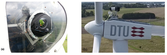
Figure 1.
Examples of the two different installation modes of the SpinnerLidar used for measuring the inflow of a wind turbine: (a) integrated in the spinner of the rotor of an NM80 wind turbine and (b) installed on the nacelle of a V52 wind turbine.
The SpinnerLidar is based on a coherent, infrared (with a 1565 nm laser wavelength), cw, Doppler lidar, which uses a monostatic transceiver with an effective radius of 24 mm and a homodyne detection scheme to detect the backscattered light. The lidar was developed by DTU Wind Energy, based on a Z300 wind lidar (ZX, U.K.), modified in order to increase the rate of the averaged Doppler spectra. The sampling of the backscattered light is held at 100 MHz, and it is used for the continuous estimation of 512-point discrete Fourier transforms (DFTs). Subsequently, a user-defined number of the absolute square DFTs are averaged to produce an average laser Doppler spectrum, which represents the power spectral density of the wind speed fluctuations along the probe volume. The probe volume is practically one-dimensional, elongated along a line-of-sight, and its full-width at half-maximum along the line-of-sight is determined by the wavelength, the effective radius of the transceiver, and the real-time adjustable focus distance [19]. The SpinnerLidar is designed to scan rapidly, using a double-prism optical scanner, a two-dimensional area covering an upwind spherical surface, which is enclosed within a cone with its apex in the spinner-mounted lidar, and with an opening angle of 30° [13]. The data acquisition configuration enables the measurement of radial wind speeds (projection of the wind vector to the line-of-sight of the lidar) up to 400-times per a second. The scanning trajectory follows a rosette pattern (see Figure 2). During the completion of one scanning pattern, the trajectory data are sampled continuously and the line-of-sight passes from certain locations more than once per scan. The highest density of measurements is found in the centre of the trajectory, where 12 measurements per scanning pattern are acquired.
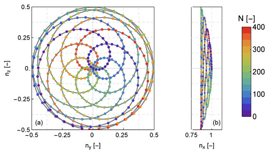
Figure 2.
(a) Front and (b) side view of the scanning pattern of the SpinnerLidar. The scanning pattern is presented in terms of the unit vector components of each line-of-sight. The colour of each line-of-sight measurement (presented with a dot) corresponds to the data acquisition order, when a sampling frequency of 200 Hz is used, in combination with a scanning duration of two seconds.
2.2. Field Study
In this study, we used SpinnerLidar data from a field study that took place at the wind turbine test station located on the Risø campus of DTU. The lidar was installed on a 850 kW wind turbine (V52, Vestas), with a 44 m hub height and a 52 m rotor diameter. Throughout the period of the field study (1 October 2020–1 August 2021), the duration of the scanning trajectory was equal to two seconds, during which the wind lidar was measuring line-of-sight speeds from a distance of 61.8 m at 200 Hz. At the time of the experiment, there were two other wind turbines at the test station in the direction of 200 in relation to Geographic North (south-southwest). The predominant wind direction at that site is west-northwest, and for that direction, wind flows over the Roskilde fjord and a flat terrain towards the wind turbine, which means that it can be considered as spatially homogeneous. In the direction of 290 and at a distance of a 115 m from the wind turbine, a meteorological mast is situated. The mast is instrumented with both cup (WindSensor P2546A-OPR) and sonic (Metek USA-1 4 Basic) anemometers at five different heights (18 m, 31 m, 44 m, 57 m, 70 m), used here to provide a reference for the wind conditions.
A common quantity that can define the quality of a velocity estimation in a cw wind lidar is the power of the detected Doppler spectral signal. In Figure 3a, we show an example of a scatter plot between the radial speed and the corresponding Doppler spectrum power denoted by P. Here, we define the power as the integrated intensity of a noise-free Doppler spectrum. The data correspond to a 10 min period when the mean wind speed, measured at 70 m, was high (10 ms) and the direction was from west-northwest. In those conditions, it is relatively straightforward to filter the blade returns using a wind speed threshold, e.g., by selecting as wind speeds only those with velocity values ms. However, when measurements are acquired during wake conditions, as is seen, for example, in Figure 3b, it is not possible to apply a speed-based criterion. Furthermore, filtering based on the maximum signal power cannot be used either, since there are many cases when the blade and aerosol signals in a Doppler spectrum have comparable contributions, as seen in both scatter plots of Figure 3. For example, in Figure 3a, the radial speeds that originate from the wind are concentrated in a point cloud with velocity values between 5 ms and 11 ms; however, the corresponding power values of this point cloud are within the range of values attributed to blade returns (<5 ms). This observation could be partially attributed to a combination of the three following circumstances: a. the beam is focused far away from the presence of the hard target; b. occasionally only a part of the cross-section of the beam is intercepted by a blade; c. the backscattering surface of the blade is not necessarily normal to the line-of-sight.

Figure 3.
Scatter plots of the radial wind speed measurements acquired over a 10 min period versus the power of the corresponding Doppler spectra for two cases when the SpinnerLidar was measuring the inflow of: (a) the free wind and (b) a wind turbine wake. The mean wind speed was the same in both cases (U = 10 ms at 70 m). The values of P represent the power of the signal, i.e., the integrated intensity of the acquired laser Doppler spectra.
Since it is not possible to differentiate between the blade and wind signals solely by the power, we propose here a method to filter these signals using the information of the rotational speed of the wind turbine. For the needs of the study, we define a 3D Cartesian right-handed coordinate system, whose x-axis is horizontal, aligned to the pointing direction of the lidar, and whose z-axis is vertical, pointing upwards. With the term pointing direction of the lidar, we mean the direction in which the line-of-sight would be emitted if no prisms were used to deflect the beam, i.e., the symmetry direction around which the rosette scanning pattern is formed. Furthermore, we assume that the scanner of the SpinnerLidar is found at the origin of the 3D Cartesian coordinate system (O).
2.2.1. Case 1: SpinnerLidar Aligned to the Centre of the Rotor
In order to understand the dependence between the position of the wind lidar and the rotor, we first consider a theoretical configuration in which the lidar is aligned to the centre of the rotor, with a displacement along the x-axis. Practically, this corresponds to an impossible configuration, which would require the wind lidar to be installed inside the nacelle and behind the rotor. However, it is going to be helpful for the understanding of the relation between the radial speed generated by a rotating blade and the measuring geometry.
Let ; here and hereinafter, vectors are denoted with bold font and unit vectors with bold font with a circumflex ( ) symbol, being the unit vector of a line-of-sight measurement of the SpinnerLidar and the vector that describes the location where a blade of the wind turbine intercepts the line-of-sight (see Figure 4a). The coordinates of will be dependent on: i. the distance along the x-axis between the location O, which corresponds to the range between the top part of the scanner of the wind lidar and the centre of the rotor plane , and ii. the vector . Since the interception of the line-of-sight by a blade happens only in the rotor plane, the vector can be expressed in terms of , scaled by a factor of , which can be written as:
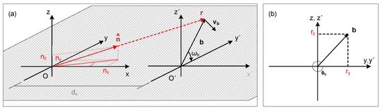
Figure 4.
Graphical illustration from (a) a perspective and (b) a front (looking towards the wind turbine) view of the coordinate system used to define the line-of-sight vector of a radial measurement at any point of a wind turbine blade rotating in the plane when the wind lidar’s pointing direction is aligned to the centre of the rotor (Case 1).
The rotational speed vector of the blade is equal to:
where is the rotational speed of a blade of the wind turbine rotor with respect to the centre of the wind turbine rotor , is the amplitude of the vector that describes the location in the rotor plane , in which the line-of-sight of the wind lidar is intercepted by the blade of the wind turbine, and is the angle between the blade and the -axis, which describes the clockwise rotation of the rotor (thus the negative sign).
When the two coordinate systems are aligned along the x-axis, then the trigonometric functions of , as seen in Figure 4b, can, by the use of Equation (1), be written as a function of the vectors and as:
and therefore when substituting these expressions into Equation (2), the radial speed , measured by the wind lidar due to the interception of the line-of-sight of the lidar by a rotating wind turbine blade is found to be zero since it is defined by the projection of the vector , Equation (2), to the , Equation (1):
2.2.2. Case 2: SpinnerLidar with an Offset from the Centre of the Rotor
When the centre of the scanning pattern has an offset along the z-axis, from the centre of the wind turbine’s rotor, as happens when a wind lidar is installed on the nacelle of a wind turbine, then the geometry of the measurement setup is as depicted in Figure 5. In this case, the trigonometric functions of the rotation of the vector are described by the following expressions:
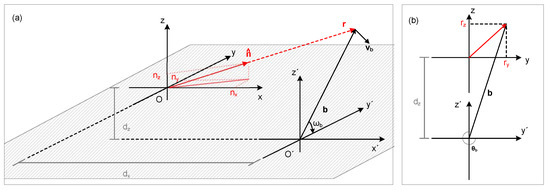
Figure 5.
Graphical illustration from (a) a perspective and (b) a front (looking towards the wind turbine) view of the coordinate system used to define the line-of-sight vector of a radial measurement at any point of a wind turbine blade rotating in the plane when the wind lidar’s pointing direction is aligned to the centre of the rotor (Case 2).
In this case, the radial speed produced by the blade is equal to:
according to which the radial wind speed is equal to the product of the rotational speed, the transverse component of the unit vector , and the vertical displacement between the two coordinate systems.
Similarly, by taking into account a displacement along the transverse axis, the radial wind speed detected by the lidar and originating from the blades is equal to:
2.2.3. Case 3: SpinnerLidar with a Misalignment Angle
In addition to the position of a nacelle wind lidar in relation to the centre of the wind turbine rotor, the alignment of the lidar has an impact on the observed radial speed generated by blade signals. The misalignment of a nacelle wind lidar can be expressed by considering three rotations around each of the axes of the coordinate system, corresponding to a roll, pitch, and yaw rotation by the angles , , and respectively, where the subscripts denote the axis of rotation. These rotations will have an impact on the unit vector of the line-of-sight, which should now be equal to .
In order to assess the impact of these rotations on the measured radial speed of a rotating blade, we performed the following sensitivity analysis. We assumed that for all the values of one scanning pattern, the SpinnerLidar is measuring only signals that originate from the blades of a wind turbine. Subsequently, we estimated the radial speed of a blade using Equation (7) for the case when a lidar is installed at a position 3 m higher and 0.3 m sideways from the centre of the rotor. We selected these values based on the consideration that the transverse displacement, which, in practice, could be attributed to the inaccuracies of the installation of the lidar, should be at least one order of magnitude less than the vertical displacement. Subsequently, we calculated the mean absolute difference between the radial wind speed using Equation (7) for an assumed perfectly aligned lidar and the ones for an assumed range of misaligned angles, between 0 and 20, for each of the three axes of the coordinate system. The results are presented in Figure 6, where we see that the largest impact is caused by a misalignment angle along the yaw direction of the wind turbine. Therefore, further analysis was only focused on the estimation of the angle.

Figure 6.
Mean absolute difference between the radial speeds generated by a wind turbine blade as measured by a SpinnerLidar configuration with no misalignment and one with a misalignment angle within 0 and 20 around the x-axis, y-axis, and z-axis.
3. Results
3.1. Determination of the SpinnerLidar Position
In order to test the performance of the blade speed model, we first selected a 10 min time period where the mean inflow wind speed at the hub height was high (10 ms at 70 m) and the wind direction was between 260 and 280, such that no wakes from the adjacent wind turbines had an impact on the measurements of the SpinnerLidar. The high wind speed range was selected to ensure that the blade signals can be easily distinguished from the wind by simply using a wind speed threshold. An example is presented in Figure 7a. In that figure, we observe two distributions of radial speeds that are split by a speed threshold of approximately 4 ms, consistent with Figure 3a. Furthermore, since is at least one order of magnitude larger than , then based on Equation (7), one should expect an almost linear relationship between and , as we see when 4 ms. Therefore, we limited the application of the model for this particular case only to those data with radial speeds less than 4 ms. In addition, measurements with transverse component values of the unit vector less than 0.1 were not used. This criterion was due to the fact that, for those unit vectors, the line-of-sight is partially back-reflected by the window that covers the two rotating prisms, which produces spurious spectral signals in the Doppler spectra. This leads to both a systematic and a random bias in the estimated radial wind speeds, the impact of which depends on the intensity of the backscattered light. The result of this error can be seen in the figure in the area < 0.1, and it is usually connected to low backscattering and low radial speed values, as, for example, can be seen in Figure 3a, where an almost constant velocity is measured for P < 1.
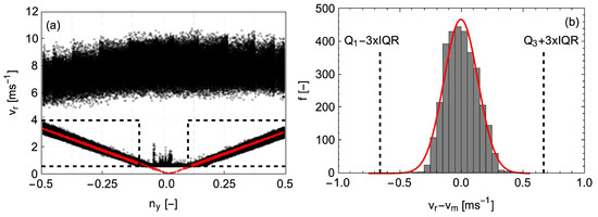
Figure 7.
(a) Radial speed measurements versus the transverse component of the line-of-sight vector. The two horizontal dashed black lines depict the two velocity limits 0.6 ms and 4 ms used to select radial speed values that are attributed to the rotating blades. The modelling of the radial speed due to the blade and the subsequent determination of the SpinnerLidar position was applied only for (depicted with two vertical dashed black lines). (b) Histogram of the differences between the measured and the modelled radial speeds using Equation (7) for the data that was acquired when .
By applying the model of Equation (7) and assuming a yaw misalignment angle of the lidar, we can estimate the values , , and using a non-linear model fit. In the histogram of Figure 7b, the difference between the measured and the modelled radial wind speed is presented for the case of . The distribution can be approximated by a Gaussian distribution. The spreading of the histogram is partially attributed to the assumption that the rotor speed is constant over a 10 min period and equal to the corresponding mean. We further observed that the estimated differences between and fall within a range within the upper and lower outer statistical fences, defined using the first (Q) and the third (Q) quartile and the interquartile range (IQR) of the distribution. As we explain in Section 3.2, we used this characteristic to form a range of acceptable deviations between and .
In order to test the accuracy of this method, we applied the same non-linear model fit procedure over 791 10-min periods with high wind speeds and a wind direction –, measured at the hub height at the meteorological mast, in order to ensure that the inflow criterion of a spatially homogeneous flow is satisfied. The results of the estimated parameters for the vertical and transverse position (relative to the centre of the rotor) are presented in Figure 8. We observed that the estimated values of these parameters from each 10 min period give results with a very low standard deviation. Specifically, we found that m and m. As expected, the transverse displacement is two orders of magnitude less than the vertical. The value of the vertical displacement is attributed to the dimensions of the mounting frame used to install the lidar on the nacelle and the distance between the centre of the rotor and the top of the nacelle. Based on the results of this model, the installation of the wind lidar had a small angle from the yaw direction equal to .
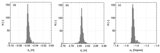
Figure 8.
Histograms of the estimated values of the (a) transverse and (b) vertical displacement, as well as of (c) the yaw alignment of the SpinnerLidar in relation to the centre of the rotor.
3.2. Data Availability
Using the estimated values of the position and the alignment of the SpinnerLidar, we can subsequently simulate what would be the radial speed of a blade for the unit vector of each line-of-sight, similar to the data presented in Figure 7a, for any period, regardless of the inflow wind conditions. In Figure 7b, we show that the difference between the modelled and the measured blade speed is described by a distribution whose characteristics are dependent on the transverse location. Using this observation, we can form a criterion in which measured speed values that have a difference from the simulated ones within the lower and upper outer fence (defined as ±3.0, the interquartile range from the first and third quartile of the distribution in different ranges of , with a width equal to 0.1) can be attributed to the rotation of the blades. Subsequently, we normalized the mean of the estimated values of the upper and lower fences for different bins of , ranging from −0.5 to 0.5, by dividing by the mean angular velocity of the rotor of each of the 791 selected periods. The average values of the fences for different values are presented in Figure 9. Based on those, we constructed a filter for identifying blade signals by re-scaling the values of each 10 min period by the corresponding mean rotation speed of the wind turbine.

Figure 9.
Mean normalized error between the modelled and the measured blade signals for different values of the transverse component of the line-of-sight vectors. The blue shaded area depicts the upper and lower outer fences of the relative difference of the two statistical quantities. The values of each 10 min period were normalized by the corresponding mean rotor speed.
Here, we used a 10 min period since it is the typical duration for estimating wind speed statistics. In Figure 10, we present with black points the 4 s time series of radial speeds of two cases when the wind lidar is measuring either in the free upwind or in the wake of another wind turbine. By assuming that the wind lidar is detecting all the time signals that originate from the rotor, we can simulate the corresponding blade speed (presented with a red line in Figure 10). Furthermore, for each measurement, we highlight the range of the maximum and minimum deviation from the theoretical modelled blade speed (presented with a red-opaque shaded area in Figure 10). Measurements that lie in that area are treated as blade speeds. In the time series, we can observe that using the suggested filtering method, we can identify which measurements originate from a blade, even in the case of wake flows that usually result in radial wind speeds similar to the ones attributed to blades.
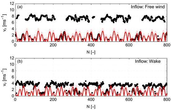
Figure 10.
Time series of radial speed measurements (black points) acquired with a 200 Hz sampling frequency. The theoretical speed, if it is assumed that the lidar is detecting all the time a rotating blade, is presented with a red line. The estimated deviation from this value due to the varying speed of the rotor within a 10 min period is marked by the red-opaque shaded area. The time series correspond to different inflow cases: ((a) free flow and (b) wake flow).
In Figure 11a, we present the total number of measurements per 10 min period for different locations in a 10 × 10 grid for a case of a free inflow. We observed that due to the motion of the rotating prisms, there are more measurements in the centre of the scanning pattern, as well as at those locations that we have more than one crossing of the scanning trajectory. In Figure 11b, we find that the data availability ranges between 57% and 89% in different locations, with a systematic decrease of the data availability in the lower part of the scanning pattern. This can be attributed to the larger cross-section of a wind turbine’s blade close to the spinner. Furthermore, we see a drop in the data availability close to the centre of the scanning pattern. This can be attributed to the spurious spectral signals occurring due to back-reflections from the window of the SpinnerLidar. The estimated data availability results for a spatial data distribution, for this case, have on average approximately 1000 measurements per grid cell over a 10 min period (see Figure 11c). Furthermore, in particular, in the centre of the scanning pattern, we find approximately 2500–3000 valid measurements.
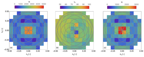
Figure 11.
(a) Number of measurements, (b) data availability, and (c) the eventual number of wind observations using a 10 × 10 grid based on the transverse and vertical components of the line-of-sight unit vector, over a 10 min period. The grey rosette pattern represents the scanning trajectory. The data corresponds to a case when the mean wind speed was 7 ms and in the direction of 256.
Subsequently, in order to study the accuracy of this method, we performed a blade detection over 12,235 10-min periods, covering a span of seven months. The 10 min periods were selected based solely on the criterion that the wind turbine was operating irrespective of the wind speed and yaw direction. In Figure 12a, we present the mean data availability, averaged over the whole scanning plane, for different yaw directions, where, in general, we can see values between 66% and 73%. In the wind direction sector between 180 and 200, we can detect that the presence of wakes reduces the data availability by 3–4%. This is attributed to wakes of the adjacent wind turbines. A similar decrease is observed in the direction between 30 and 60. This decrease is associated with an increase of the standard deviation, which indicates that the reduction of the mean data availability is attributed to a few cases with low values (approximately 50–60%). No correlation was found for these cases with mean wind speed, rotational speed of the rotor, or time. However, in that direction sector and at a distance of 70 m, there is a group of buildings with a height of approximately 4 m, which could occasionally introduce a vertical variation of the wind profile and, thus, have an impact on the estimated data availability. Overall, we observed that the method provides systematic results regardless of the yaw direction, and thus the inflow conditions. This is good news, since it means that the presence of wakes has no significant impact on the performance of this method. Furthermore, we observed a slight increase of the data availability with the rotational speed of the rotor (see Figure 12b).
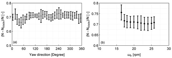
Figure 12.
Mean data availability, defined here by the relative difference between the total amount of measurements N and the number of blade signals detected per (a) yaw direction and (b) rotor speed, over a 10 min period. The error bars correspond to one standard deviation about the mean.
Using the filtered data, we then compared both the estimated magnitude of the mean horizontal wind vector, as well as the corresponding yaw misalignment of the wind turbine. For this purpose, we selected 1601 10-min periods from 8 October 2020 23:00 (UTC+1) to 20 November 2020 12:00 (UTC+1), when the wind direction was between and . In this direction sector, no shadowing effects from the structure of the mast are expected on the cup measurements. In this analysis, we focused only on those measurements acquired between 42 and 46 m, in order to compare the SpinnerLidar measurements to the ones of the meteorological mast at the hub height, when taking into account the two-meter elevation offset of the ground above mean sea level between the location of the mast and the wind turbine. For the estimation of the mean wind speed and direction, we used the mean line-of-sight unit vector of the lidar, and by assuming that the mean vertical component of the wind vector is negligible, we express the radial wind speeds of the lidar as , where u and v denote the longitudinal and lateral component of the wind vector. Subsequently, using a non-linear model fit, we first estimated the values of u and v and, then, the mean speed U and direction of the wind. We observed that the yaw misalignment, defined here as the difference between the measured wind direction at 44 m at the mast and the yaw direction of the wind turbine, is equal to 0.8 with a standard deviation of 3.8. Similarly, based on the wind lidar measurements, the horizontal wind vector in relation to the alignment of the SpinnerLidar has a mean angle of 0.7 and a standard deviation of (see Figure 13a). Furthermore, we observed a high correlation (Pearson correlation coefficient r > 0.98) between the magnitude of the 10 min mean horizontal wind vector measured by the wind lidar and the cup anemometer at the meteorological mast, which is associated with a low bias (< ms) (see Figure 13b).
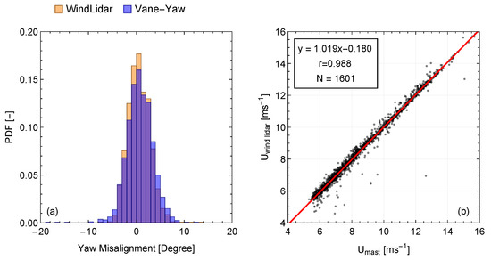
Figure 13.
(a) The histogram of the yaw misalignment estimated using the measurements of the wind direction at the meteorological mast and the yaw direction of the wind turbine. (b) Scatter plot of the magnitude of the mean horizontal wind speed vector measured by a cup anemometer (U) and the SpinneLidar (U) at 44 m.
4. Discussion
The accuracy of this blade filtering method would be higher if the nacelle wind lidar was synchronized with the supervisory control and data acquisition (SCADA) of the wind turbine. This way, we would not have to assume that the rotational speed is constant over a 10 min period, and thus, the spread of the difference between the measured and model blade speed (example in Figure 7) would be narrower. This hypothesis is supported when examining the following case. If we use Equation (7) for a fixed value of the transverse vector = 0.5 and estimate the blade speed using the 50 Hz data of the rotational speed of the wind turbine over a 10 min period (see Figure A1), then we see a distribution with a mean speed equal to 3.26 ± 0.22 ms, where the deviation about the mean corresponds to one standard deviation (see Figure 14b). Similarly, if we select the radial measurements from the wind lidar that correspond to the blade speed for = 0.5 (749 cases over the same 10 min period), we observe that the resulting distribution (see Figure 14a) has a mean equal to 3.26 ± 0.26 ms. This shows that a big part of the variability between the measured and modelled blade speed is attributed to the variations of the rotor speed.

Figure 14.
Estimated values of the blade speed based on (a) the lidar measurements and (b) the modelled values of Equation (7) using a varying rotational speed of the wind turbine’s rotor.
Using the method presented in this paper, one can increase the reliability of nacelle-mounted cw Doppler lidar data and, thus, increase the accuracy of the retrieved spatio-temporal statistics of wind. This is important not only for studying the characteristics of the flow, but also in the case of load validation in the wake conditions, as was demonstrated in the theoretical studies of Conti et al. [14] and Dimitrov et al. [20], who showed that using the measurements of a nacelle scanning wind lidar, it is possible to perform an accurate load validation.
The method for filtering the nacelle wind lidar measurements using a predictive model of the radial velocities of the blades is not limited to the case of a scanning nacelle wind lidar as the SpinnerLidar, but it can be also used in data acquired by wind lidars that are scanning in simpler trajectories, as the commercial ZX TM – Turbine Mounted wind Lidar (ZX, U.K.), which is designed to sample 50 measurements around the periphery of circle, whose radius is determined by the focusing distance and the deflection angle of a rotating prism, which is equal to either 15 or 30. In order to study the accuracy of a nacelle lidar with such a measuring configuration, we selected only those SpinnerLidar measurements that were acquired with deflection angles of 15 and 30 (see Figure A2 in the Appendix B). The results show that the determination of the position of the lidar is the same irrespective of the value of the conical scanning angle. We found m, m, and and m, m, and for , , and , for the cases of 15 or 30, respectively. These results are approximately equal to the estimations using the full scanning trajectory of the SpinnerLidar.
5. Conclusions
In this study, we presented a lidar data filtering method using a predictive model of the radial speed of the wind turbine blade based on the rotational speed of the rotor, the location of the nacelle wind lidar relative to the centre of the rotor, and the alignment of the nacelle wind lidar relative to the rotational plane of the wind turbine. Using the estimated parameters, we could simulate the radial speed produced by the blades for all situations regardless of the wind speed and direction. We tested this method using data acquired by a cw wind lidar, which was installed on a V52 wind turbine. We found that the mean data availability varied between 70 and 73% for the cases of a free inflow. This result was slightly decreased in the case of a complex inflow (i.e., wake). This is positive news since it shows that, even in the case of a complex inflow (e.g., wake of an adjacent wind turbine), the application of this method does not present a systematic bias that could be attributed to the spatial variations of the inflow. The method presented can also be used to improve the accuracy of the alignment of the nacelle-mounted cw Doppler lidar to the wind turbine rotor and, thus, improve the monitoring of the yaw misalignment. The high sampling frequency of the SpinnerLidar in combination with the estimated data availability supports the use of such an instrument to study not only the mean properties of the inflow, but also the second-order moments of the wind. The impact of the method presented here is dependent on the climatology and the location of the wind turbine. In the case of a wind turbine that is situated in an area with mean wind speeds that are comparable to the blade signals or within a wind farm, where the wakes of the adjacent wind turbines are likely to distort the inflow conditions, the blade filtering will be very useful to distinguish between the wind and blade signals. Furthermore, the suggested method would increase the data availability in the case of measuring during rain events, which would facilitate the study of rain characteristics using nacelle-mounted wind lidars.
Author Contributions
Conceptualization, N.A. and M.S.; methodology, N.A. and M.S.; data analysis, N.A.; investigation, N.A. and M.S.; writing—original draft preparation, N.A.; writing—review and editing, N.A. and M.S.; visualization, N.A. All authors have read and agreed to the published version of the manuscript.
Funding
This research received no external funding.
Data Availability Statement
Not applicable.
Conflicts of Interest
The authors declare no conflict of interest.
Appendix A. Example of the Variability of the Rotational Speed of the Rotor of Wind Turbine
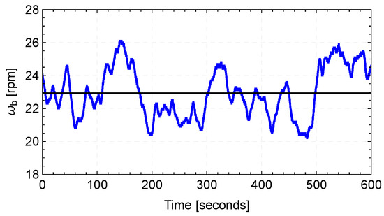
Figure A1.
Example of the 50 Hz time series of the rotational speed of the wind turbine’s rotor for a case with a free inflow.
Appendix B. Conically Scanning Nacelle Wind Lidars
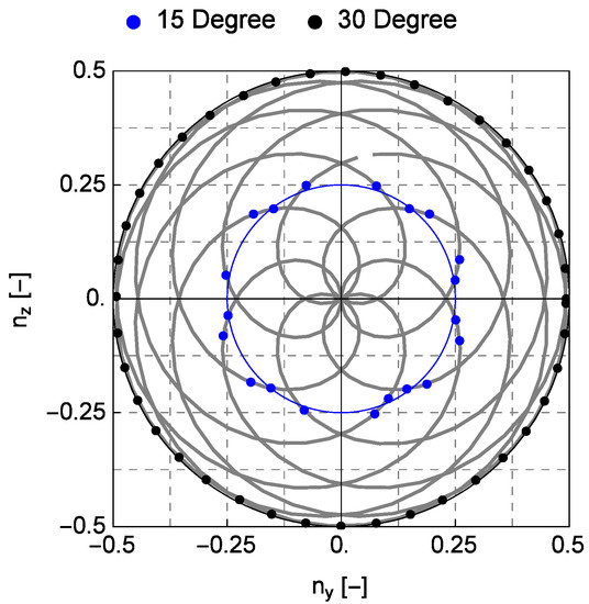
Figure A2.
Scanning pattern of the SpinnerLidar, depicted in grey, and points selected from the scanning pattern in order to reproduce the measurements of a conically scanning wind lidar with an opening angle of either 15 or 30, depicted in blue and black, respectively.
References
- Wiser, R.; Rand, J.; Seel, J.; Beiter, P.; Baker, E.; Lantz, E.; Gilman, P. Expert elicitation survey predicts 37% to 49% declines in wind energy costs by 2050. Nat. Energy 2021, 6, 555–565. [Google Scholar] [CrossRef]
- Harris, M.; Bryce, D.J.; Coffey, A.S.; Smith, D.A.; Birkemeyer, J.; Knopf, U. Advance measurement of gusts by laser anemometry. J. Wind Eng. Ind. Aerodyn. 2007, 95, 1637–1647. [Google Scholar] [CrossRef]
- Borraccino, A.; Schlipf, D.; Haizmann, F.; Wagner, R. Wind field reconstruction from nacelle-mounted lidar short-range measurements. Wind Energy Sci. 2017, 2, 269–283. [Google Scholar] [CrossRef] [Green Version]
- Held, D.P.; Mann, J. Detection of wakes in the inflow of turbines using nacelle lidars. Wind Energy Sci. 2019, 4, 407–420. [Google Scholar] [CrossRef] [Green Version]
- Sonnenschein, C.M.; Horrigan, F.A. Signal-to-Noise Relationships for Coaxial Systems that Heterodyne Backscatter from the Atmosphere. Appl. Opt. 1971, 10, 1600. [Google Scholar] [CrossRef] [PubMed]
- Gryning, S.E.; Floors, R. Carrier-to-Noise-Threshold Filtering on Off-Shore Wind Lidar Measurements. Sensors 2019, 19, 592. [Google Scholar] [CrossRef] [PubMed] [Green Version]
- Dabas, A.M.; Drobinski, P.; Flamant, P.H. Velocity Biases of Adaptive Filter Estimates in Heterodyne Doppler Lidar Measurements. J. Atmos. Ocean. Technol. 2000, 17, 1189–1202. [Google Scholar] [CrossRef]
- Beck, H.; Kühn, M. Dynamic Data Filtering of Long-Range Doppler LiDAR Wind Speed Measurements. Remote Sens. 2017, 9, 561. [Google Scholar] [CrossRef] [Green Version]
- Alcayaga, L. Filtering of pulsed lidar data using spatial information and a clustering algorithm. Atmos. Meas. Tech. 2020, 13, 6237–6254. [Google Scholar] [CrossRef]
- Herges, T.G.; Keyantuo, P. Robust Lidar Data Processing and Quality Control Methods Developed for the SWiFT Wake Steering Experiment; IOP Publishing: Visby, Sweden, 2019; Volume 1256, p. 012005. [Google Scholar] [CrossRef]
- Angelou, N.; Sjöholm, M. UniTTe WP3/MC1: Measuring the Inflow towards a Nordtank 500kW turbine using three short-range WindScanners and one SpinnerLidar; Report DTU Wind Energy E-0093; DTU Wind Energy: Roskilde, Denmark, 2015. [Google Scholar]
- Mikkelsen, T.; Angelou, N.; Hansen, K.; Sjöholm, M.; Harris, M.; Slinger, C.; Hadley, P.; Scullion, R.; Ellis, G.; Vives, G. A spinner-integrated wind lidar for enhanced wind turbine control. Wind Energy 2013, 16, 625–643. [Google Scholar] [CrossRef] [Green Version]
- Sjöholm, M.; Pedersen, A.T.; Angelou, N.; Abari, F.F.; Mikkelsen, T.; Harris, M.; Slinger, C.; Kapp, S. Full two-dimensional rotor plane inflow measurements by a spinner-integrated wind lidar. In Proceedings of the European Wind Energy Conference & Exhibition, Vienna, Austria, 4–7 February 2013. [Google Scholar]
- Conti, D.; Dimitrov, N.; Peña, A.; Herges, T. Wind Turbine Wake Characterization Using the SpinnerLidar Measurements; IOP Publishing: Torque, The Netherlands, 2020; Volume 1618. [Google Scholar] [CrossRef]
- Herges, T.G.; Maniaci, D.C.; Naughton, B.T.; Mikkelsen, T.; Sjöholm, M. High resolution wind turbine wake measurements with a scanning lidar. J. Physics Conf. Ser. 2017, 854, 012021. [Google Scholar] [CrossRef] [Green Version]
- Mikkelsen, T.; Sjöholm, M.; Astrup, P.; Peña, A.; Larsen, G.; van Dooren, M.F.; Sekar, A.P.K. Lidar Scanning of Induction Zone Wind Fields over Sloping Terrain; NAWEA WindTech; IOP Publishing: Amherst, MA, USA, 2020; Volume 1452, p. 012081. [Google Scholar] [CrossRef]
- Peña, A.; Mann, J.; Rolighed Thorsen, G. SpinnerLidarmeasurements for the CCAV52; Report DTU Wind Energy E-0177; DTU Wind Energy: Roskilde, Denmark, 2019. [Google Scholar]
- Fu, W.; Peña, A.; Mann, J. Turbulence statistics from three different nacelle lidars. Wind Energy Sci. Discuss. 2021, 2021, 1–29. [Google Scholar] [CrossRef]
- Angelou, N.; Mann, J.; Sjöholm, M.; Courtney, M. Direct measurement of the spectral transfer function of a laser based anemometer. Rev. Sci. Instrum. 2012, 83, 033111. [Google Scholar] [CrossRef] [PubMed] [Green Version]
- Dimitrov, N.; Borraccino, A.; Peña, A.; Natarajan, A.; Mann, J. Wind turbine load validation using lidar-based wind retrievals. Wind Energy 2019, 22, 1512–1533. [Google Scholar] [CrossRef]
Publisher’s Note: MDPI stays neutral with regard to jurisdictional claims in published maps and institutional affiliations. |
© 2022 by the authors. Licensee MDPI, Basel, Switzerland. This article is an open access article distributed under the terms and conditions of the Creative Commons Attribution (CC BY) license (https://creativecommons.org/licenses/by/4.0/).