Article

Physics-Driven Deep Learning Inversion with Application to Magnetotelluric

1
Key Laboratory of Metallogenic Prediction of Nonferrous Metals and Geological Environment Monitoring (Ministry of Education), Central South University, Changsha 410083, China
2
Hunan Key Laboratory of Nonferrous Resources and Geological Hazards Exploration, Central South University, Changsha 410083, China
3
School of Geosciences and Info-Physics, Central South University, Changsha 410083, China
*
Author to whom correspondence should be addressed.
Remote Sens. 2022, 14(13), 3218; https://doi.org/10.3390/rs14133218
Submission received: 21 May 2022 / Revised: 27 June 2022 / Accepted: 30 June 2022 / Published: 4 July 2022

Abstract

:
Due to the strong capability of building complex nonlinear mapping without involving linearization theory and high prediction efficiency; the deep learning (DL) technique applied to solve geophysical inverse problems has been a subject of growing interest. Currently, most DL-based inversion approaches are fully data-driven (namely standard deep learning), the performance of which largely depends on the training sample sets. However, due to the heavy burden of time and computational resources, it can be challenging to supply such a massive and exhaustive training dataset for generic realistic exploration scenarios and to perform network training. In this work, based on the recent advances in physics-based networks, the physical laws of magnetotelluric (MT) wave propagation is incorporated into a purely data-driven DL approach (PlainDNN) and thus builds a physics-driven DL MT inversion scheme (PhyDNN). In this scheme, the forward operator modeling MT wave propagation is integrated into the network training loop, in the form of minimizing a hybrid loss objective function composed of the data-driven model misfit and physics-based data misfit, to guide the network training. Consequently, the proposed PhyDNN method will take the advantage of the fully data-driven DL and conventional physics-based deterministic methods, allowing it to deal with complex realistic exploration scenarios. Quantitative and qualitative analysis results demonstrate that the PhyDNN can honor the physical laws of the MT inverse problem, and with other conditions unchanged, the PhyDNN outperforms the PlainDNN and the classical deterministic Occam inversion method. When processing field data, the PhyDNN method yields considerably impressive inversion results compared to the Occam method, and the corresponding simulated MT responses agree well with the real measurements, which confirms the effectiveness and applicability of the PhyDNN method.

1. Introduction

The Magnetotelluric (MT) method, as a remote sensing tool for the subsurface, has been widely applied in geophysical prospecting scenarios, such as crust imaging, geothermal exploration, and mineral, oil and gas exploration. This method images the subsurface structures by inverting the collected natural geomagnetic and geoelectric fields at the Earth’s surface [1,2]. Because inversion plays a critical role in the accurate estimation of subsurface properties, it has been well studied by exploration geophysicists in the past few decades. In general, mainstream MT inversion methods can be categorized into two groups: deterministic and statistical inversion methods. The former, based on linearization theory, such as Occam [3,4], nonlinear conjugate gradient [5,6] and Gauss–Newton [7,8] methods, iteratively solves a nonlinear optimization problem by minimizing a so-called objective function (the data residual/misfit between the actual measurements and synthetic responses in a L 2 norm). The deterministic methods are efficient to search for the best earth model, but usually suffer from the local optima problem and are sensitive to the initial model. The statistical methods [9,10,11] convey the posterior probability distributions of parameters by conditioning the model response on the measurements and providing an assessment of non-uniqueness. These methods do not require linearizing the inverse problem, and thus they are particularly desirable for highly nonlinear problems. However, they often perform hundreds of forward simulations, which are extremely time-consuming and demand extensive process power for large surveys. Along with all these challenges, the aforementioned methods need to repeat the entire inversion process for each new measurement dataset, which can be computationally intensive.
In recent years, using deep learning (DL) techniques to solve inverse problems has been a topic of growing interest. In the DL inversion scheme, the basic idea is to train a deep neural network (DNN) to approximate the inverse operator Γ 1 . DL has a strong ability to build complex nonlinear mapping from data (input) to models (output) without involving linearization theory. Although the training process of a DNN may be time-consuming, once the network is properly trained, it possesses extremely high inversion efficiency, which is significantly convenient and practical for large surveys. For example, Araya-Polo et al. [12] used a DNN to produce accurate tomography inversion. Das et al. [13] proposed a framework based on a convolutional neural network (CNN) to realize seismic impedance inversion successfully. Puzyrev [14] demonstrated that a CNN can be trained to realize onshore carbon dioxide reservoir imaging using controlled source electromagnetic (CSEM) data. Bai et al. [15] realized instantaneous inversion of airborne time-domain electromagnetic data via DNN. Wu et al. [16] performed one-dimensional (1D) DL inversion for airborne transient electromagnetic data using CNN. For MT inversion, Wang et al. [17] developed a DL inversion strategy based on a deep belief network for MT resistivity imaging. Liu et al. [18] applied a deep residual CNN for audio magnetotelluric (AMT) 1D inversion. However, the aforementioned DL-based inversion approaches are fully data-driven and thus the network performance largely depends on the training dataset. A fully data-driven DL framework trained on an insufficient training dataset may not be able to accurately reconstruct the nonlinear mapping between the data and models. In other words, it cannot completely honor the physical laws of the inverse problem (e.g., electromagnetic wave propagation). These purely data-driven DL approaches require massive representative training sets to build robust networks and ensure good generalization capability. Nevertheless, supplying such large and rich data sets could be challenging. Due to the heavy burden of time and computational power, it is difficult to build a set of complex synthetic models (e.g., resistivity models) and generate the corresponding forwarding responses for generic realistic exploration scenarios, and perform training. This in turn may make DL inversion methods less appealing compared to conventional deterministic inversion.
A very recent trend is to impose the physics into the DL inversion scheme to control the network training process. For instance, Adler and Oktem [19] performed conventional iterative inversion using a well-trained CNN to adjust the gradients produced by the gradient-descent algorithm for each successive iteration. Raissi et al. [20] employed the physics constraint as a regularization term and added it to the loss objective function. Fuks and Tchelepi [21] embedded the initial and boundary conditions in a composite loss function and performed training on smaller datasets. Colombo et al. [22] incorporated DL techniques into standard deterministic inversion schemes to obtain better, more stable and unique transient electromagnetic (TEM) inversion results. Inspired by the conventional inversion considering the governing wave equation, some other works incorporated the physical laws of the inverse problem into the DL inversion architecture. For example, Sun et al. [23] constructed an RNN-based forward operator Γ to emulate wave propagation and implemented unsupervised DL seismic inversion, of which the training process is equivalent to the optimization of conventional deterministic inversion methods. Wang et al. [24] developed a closed-loop framework based on 1D CNN to model the seismic inversion and forward process simultaneously, and the forward process is responsible for providing theoretical constraints for the inversion process. In this way, the incorporation of physics could not only lead to a more reasonable and stable updating direction of parameters but also reduce the dependency on an exhaustive training dataset.
In this work, the physical laws of MT wave propagation are incorporated into the purely data-driven approach and a physics-driven DL MT inversion scheme is constructed. In this scheme, the MT forward operator Γ simulating wave propagation is imposed into the DL inversion architecture to help guide the network training by constructing a hybrid loss function composed of the data-driven model misfit and physics-based data misfit. The model misfit is the difference between the true models to the predicted models. The data misfit is the difference between the measurements (input) and the forward responses calculated by Γ from the predicted models. In fact, the conventional deterministic inversion methods rely on the Γ and usually adopt the data misfit (or plus regularization term) as the objective function to guide its search for the optimal solution. Therefore, the proposed physics-driven DL inversion approach will benefit from both the fully data-driven DL and deterministic methods, enabling it to reduce the dependency on extensive training sets and to have the ability to deal with complex realistic exploration scenarios. To our best knowledge, the MT inversion using such a physics-driven DL inversion scheme has not been reported in the literature. This novel DL inversion method is demonstrated in both synthetic and field MT cases, and it is expected to have promising application effects.

2. Methodology

2.1. Problem Statement

The MT method is used to reflect the subsurface geological structures by imaging the spatial variation of the resistivity (or the equivalent conductivity) of the underground medium. Since 3D MT forward modeling is a heavy burden of computational cost, it is significant and practical to adopt 1D parameterization modeling and inversion in fieldwork for instantaneous data interpretation and decision-making. It is common to stitch the 1D inversion results together to form a pseudo-2D (or pseudo-3D) subsurface image. Moreover, 1D inversion results delivering horizontally layered models of resistivity versus depth can provide a fundamental understanding of the subsurface structure for the survey area in advance and then facilitate moving on to realistic 3D problems.
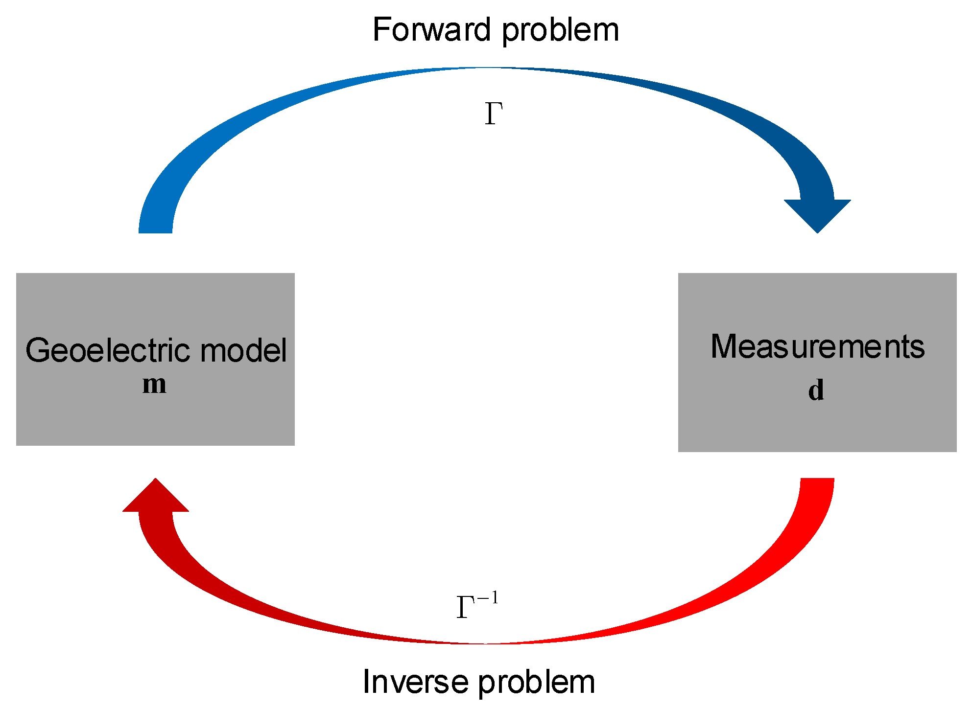
From the viewpoint of mathematics, two crucial MT problems illustrated in Figure 1 are introduced below.
Forward problem: Given a known geoelectric model (which, in our paper, is represented by the vector m for the resistivity distribution of the medium), the MT forward modeling delivers the electric and magnetic fields, namely simulated MT responses (in our case, the derived apparent resistivity and phase are employed and denoted as a vector d ^ ) at stations. The forward problem can then be expressed as follows:
d ^ = Γ ( m ) ,
where Γ is the forward operator based on Maxwell’s equations governing the electromagnetic wave propagation phenomena. It is composed of an operator to calculate the analytical electromagnetic responses and an operator to compute the apparent resistivities and phases from the electric field and magnetic fields.
Inverse problem: Given a group of measurements d (real MT responses) acquired at stations, the inverse problem can be formulated as an optimization problem aimed at finding the optimal model m ^ that matches the measurements d . This can be described by the following expressions:
m ^ = Γ 1 ( d ) ,
where Γ 1 denotes the generalized inverse operation of the forward operation Γ .
In the conventional deterministic inversion process, an optimization method is employed to iteratively improve the estimated geoelectric model m ^ until the difference between the measurements d and the simulated MT responses d ^ from m ^ meets the misfit tolerance. In the presented work, it is intended to approximate the inverse function Γ 1 using a physics-driven DL approach. When training is well conducted, the network can be regarded as a generalized function that directly maps the input (apparent resistivity and phase) to the output (resistivity model), and the process of inversion can be carried out to instantly predict the subsurface property distribution.

2.2. Network Architecture

The DL inversion workflow is comprised of three steps, namely sample data generation, network designing and training, and network prediction. These three steps jointly determine the performance of the DL inversion. Hence, it is of significance to build a reliable and efficient DNN model.
The built DNN model in this work combines the prevalently used U-Net [25] and residual network (ResNet) [26] architectures. The U-Net is based on a fully CNN [27] and consists of an encoder (or down-sampling) and a decoder (or up-sampling) part, and is well-known for its skip connection operation, which concatenates the low-level feature from the shallow layer (encoder part) to the high-level feature from the deep layer (decoder part). It, together with convolution and deconvolution, enables the U-Net to have better localization and feature representation capabilities and allows fewer training samples, compared to other fully CNNs. The ResNet is built on the concept of shortcut connection and can overcome the gradient vanishing and network degradation problems when the network depth considerably increases.
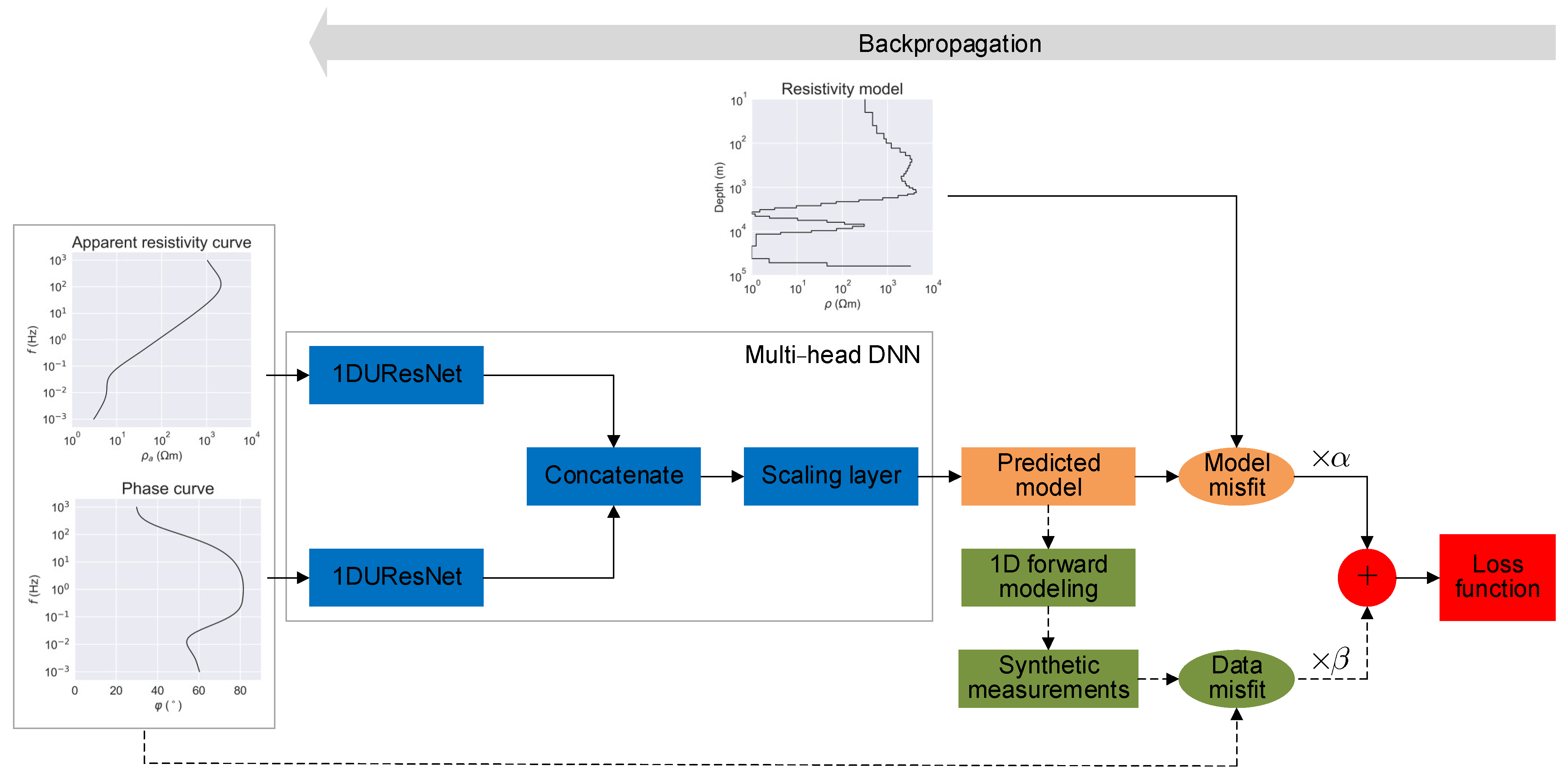
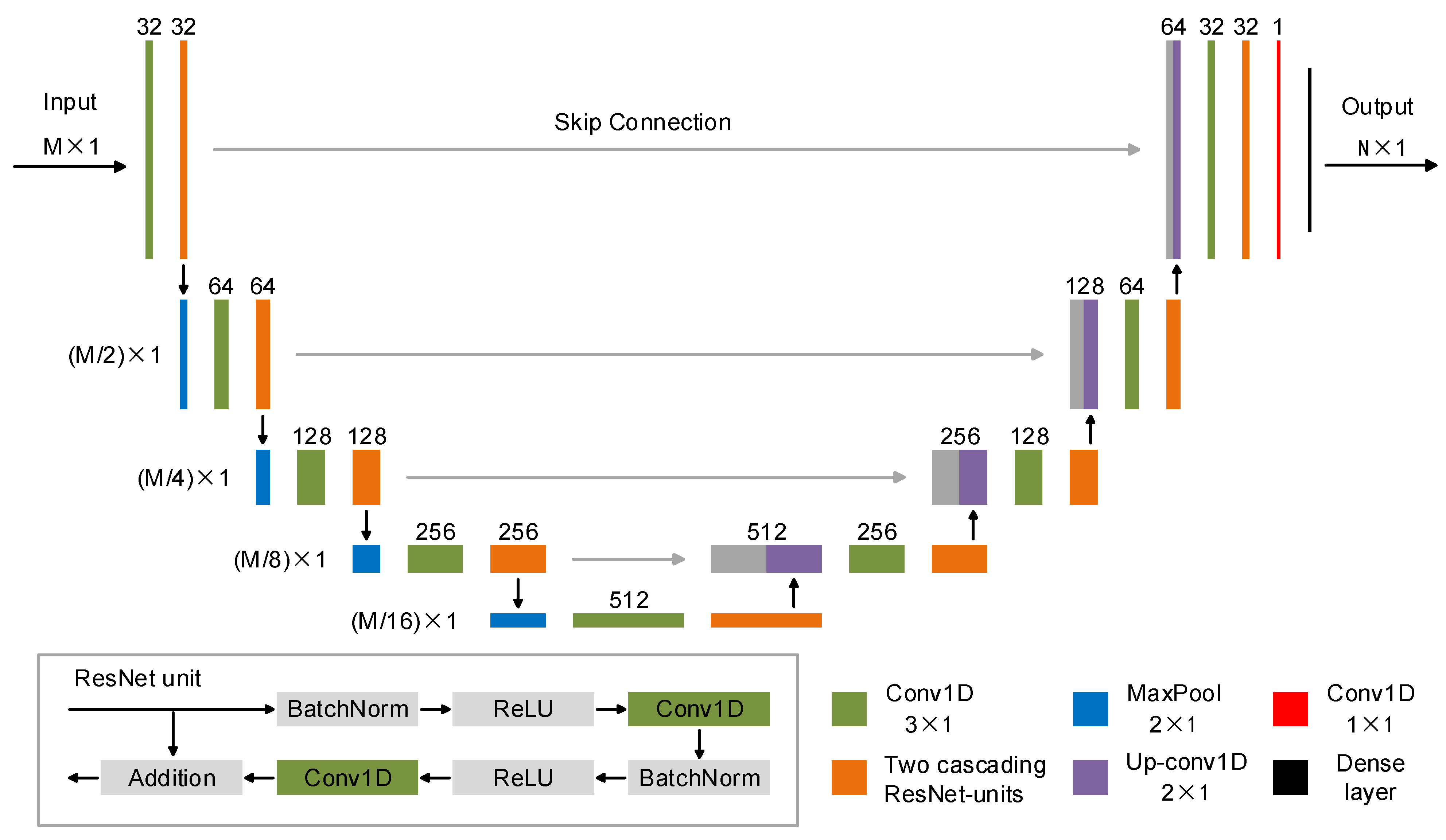
As illustrated in Figure 2, to adapt to our 1D MT inverse regression problem, a Unet-like 1D CNN model (1DUResNet) is designed and built by embedding the ResNet unit into the U-Net architecture. The encoder path on the left side consists of four down-sampling blocks. In every block, each repeated convolutional layer (3 × 1 kernel, 1 stride, ‘SAME’ padding) is followed by two cascading ResNet units (3 × 1 kernel, 1 stride, ‘SAME’ padding) and a max-pooling operation (2 × 2 kernel, 2 stride). The number of feature channels increases from 32 to 512. The decoder path on the right side consists of four up-sampling blocks. Each block is composed of a deconvolution operation (3 × 1 kernel, 2 stride, ‘SAME’ padding) and a concatenation operation of low-level and high-level features, followed by a convolutional layer and two cascading ResNet units. In the last block, a convolutional layer (1 × 1 kernel, 1 stride, 1 channel, ‘SAME’ padding) and a dense layer (50 neurons) are added to adjust the network output to match the desired output. The input and output sizes are 128 × 1 and 50 × 1, respectively. In order to reduce overfitting and improve generalization ability, the dropout operation (0.1 ratio) after the max-pooling operation is applied in the encoder part and the concatenation operation in the decoder part, to regulate the learning process.

2.3. Physics-Driven DL Inversion Scheme

Most DL-based methods for solving MT inverse problems are fully data-driven. These methods take the model misfit m that measures the difference between the true models m and the predicted models m ^ as the loss objective function Φ :
Φ ( d , m , θ ) = m ( m ^ , m ) = 1 T N i = 1 T j = 1 N ( m ^ i j m i j ) 2 = 1 T N i = 1 T j = 1 N ( H ( d , θ ) i j m i j ) 2
where T is the number of sample pairs ( d , m ) involved in training, N is the number of model parameters, d is the measurements, and H is the feed-forward network parameterized by θ . During the training process, the network performs the learning by minimizing the loss function Φ , (written as):
θ ^ = arg min θ Φ ( d , m , θ )
Once the network is well trained, the feed-forward network H can be used as an inverse operator, Γ 1 , to produce predictions, m ^ , from a new set of measurements, d .
Though a fully data-driven DL approach can be a powerful tool to solve the MT inverse problem, it requires an exhaustive synthetic training dataset related to the exploration scenario to build robust networks and ensure good generalization ability. Unlike the purely data-driven DL methods, a physics-driven DL inversion scheme by integrating the 1D forward operation Γ modeling MT wave propagation into the DNN training loop is proposed in this work. As shown in Figure 3, in this scheme, the loss objective function is a weighted sum of model misfit m and physics-based data misfit d . The data misfit d measures the difference between the measurements d and the simulated MT responses d ^ calculated by Γ from the predicted models m , defined as:
d ( d ^ , d ) = 1 T M i = 1 T j = 1 M ( d ^ i j d i j ) 2 = 1 T M i = 1 T j = 1 M ( Γ ( m ^ ) i j d i j ) 2 = 1 T M i = 1 T j = 1 M ( Γ ( H ( d , θ ) ) i j d i j ) 2
where M is the number of measurement parameters. Then, the loss objective function Φ controlling the network training is as follows:
Φ ( d , m , θ ) = α m ( m ^ , m ) + β d ( d ^ , d ) = α 1 T N i = 1 T j = 1 N ( H ( d , θ ) i j m i j ) 2 + β 1 T M i = 1 T j = 1 M ( Γ ( H ( d , θ ) ) i j d i j ) 2
where the weighted parameters
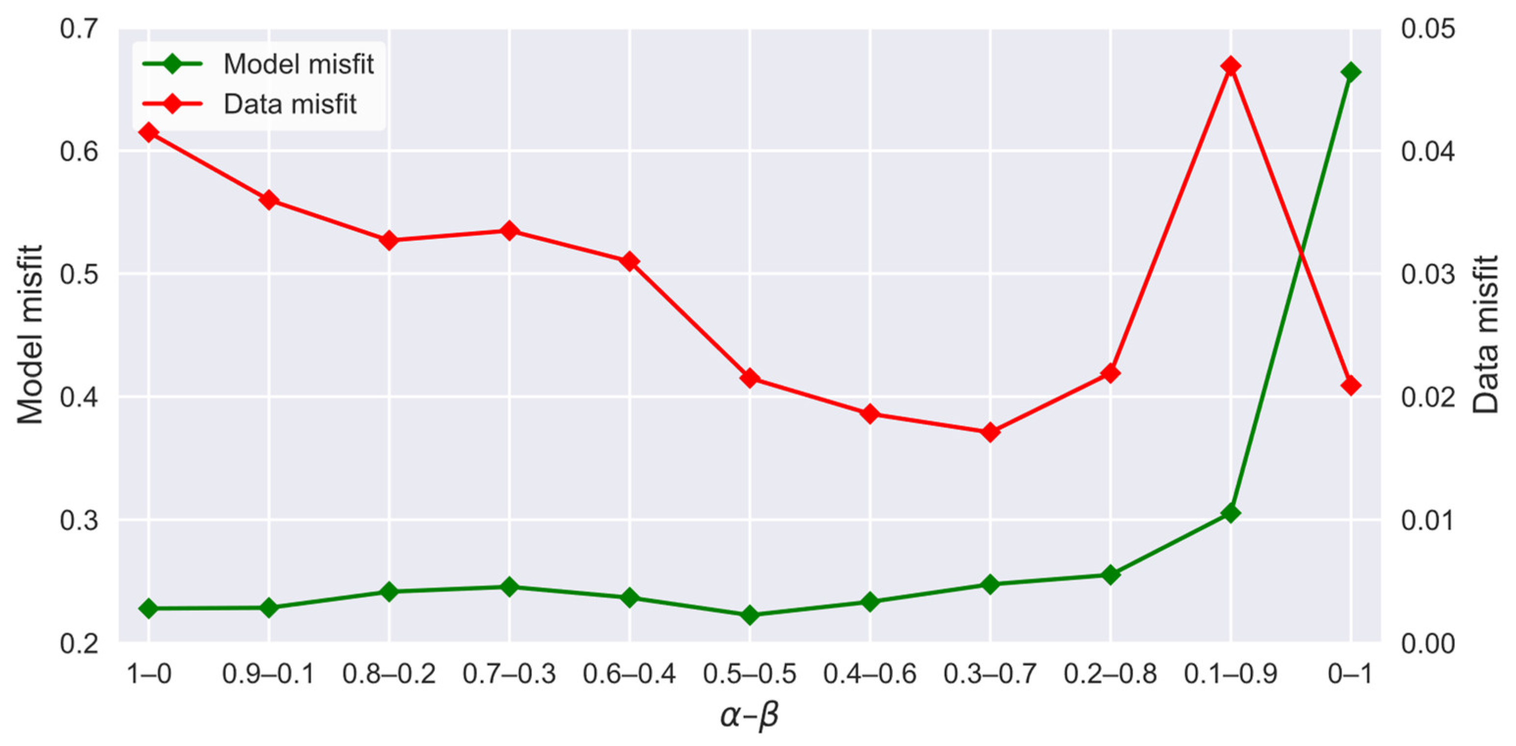
 α , β are used to balance the relative contributions of the two misfit terms and are both set to 0.5 in our work.
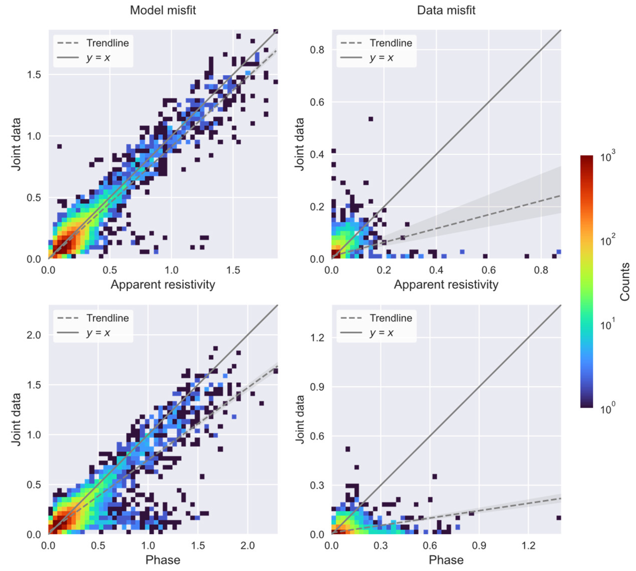
Unlike other MT DL inversion works [17,18] which used the apparent resistivity as network input alone, both the apparent resistivity and phase derived from measurements are employed for inversion. Liu et al. [17] have demonstrated that the network performance is worse using the concatenation of apparent resistivity and phase than individual apparent resistivity as input, due to the significant difference between the apparent resistivity (usually covers several orders of magnitude) and the phase (between 0 and 90). Hence, a multi-head DNN is constructed as shown in Figure 3, which consists of two individual network paths based on 1DUResNet with each using apparent resistivity and phase as input, respectively. Then the outputs of two paths are transferred to the scaling layer after the concatenation operation. The scaling layer serves as the prior knowledge to constrain the predictions to a proper value range and is defined as:
H s ( m ^ c , θ s ) = ( m max m min ) sigmoid ( θ s m ^ c ) + m min
where H s denotes the scaling layer parameterized by θ s , m ^ c is the preceding concatenation result, m max , m min represent the predetermined upper and lower bounds of predictions, respectively.
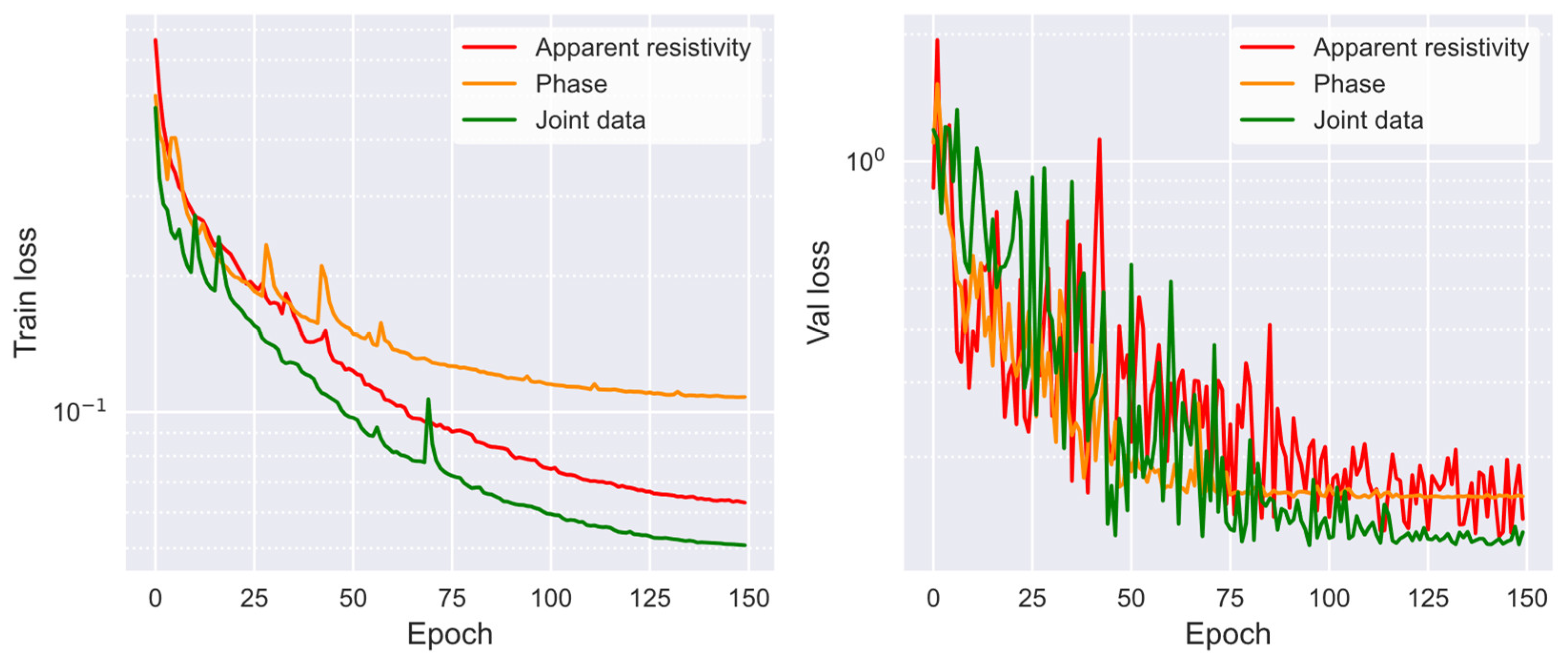
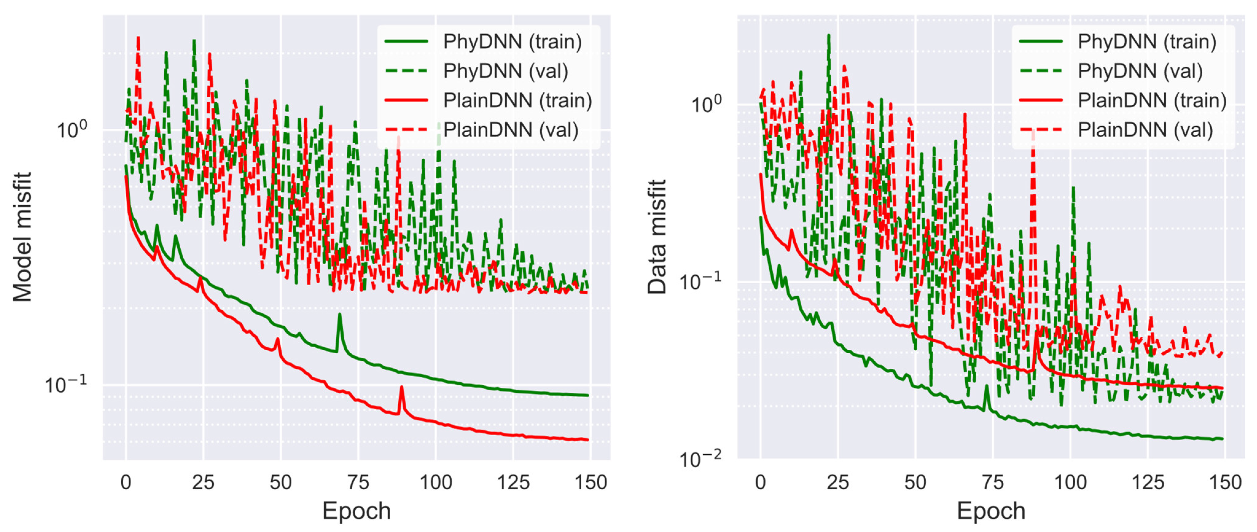
Compared to the purely data-driven DL (PlainDNN), the proposed physics-driven DL (PhyDNN) scheme will reduce the dependency on exhaustive training sets and produce more accurate, stable and reliable inversion results. During the DL training, the early-stopping technique with a patience of 50 (total epochs of 150 in our following work) is used to avoid overfitting the training data. The popular Adam optimization algorithm is employed to minimize the loss objective function with a batch size of 128. In order to accelerate the convergence and prevent the DNN from falling into local optima prematurely, a dynamic learning rate scheme that the learning rate will decrease by a factor of 0.8 if the loss on the validation sets fails to reduce or remains constant for five consecutive epochs is adopted. The implementation is based on TensorFlow using a desktop (system: Intel(R) Core (TM) i7-9700 CPU @ 3.00GHz, 16.9 GB RAM. GPU: GeForce RTX3060 with 8G VRAM).

2.4. Sample Data Generation

Sample data generation is a key step of DL-based inversion methods. Though the generation of 1D MT data typically does not pose significant problems because of the low number of model parameters and the availability of analytical solutions, it could be time-consuming to perform network training using an extremely massive dataset. Hence, it is necessary to construct a reasonable-sized and high-quality sample dataset. In the presented work, the number and thickness of layers for all synthetic resistivity models are fixed. The number of layers is set to 50 and the bottom depth of the models is 50 km. The thickness of layers is set following Krieger and Peacock [28], with 44 layers within the 10 km target depth and five extended layers between the target depth and bottom depth. The deepest layer that is below 50 km is a uniform half-space whose thickness is infinite.
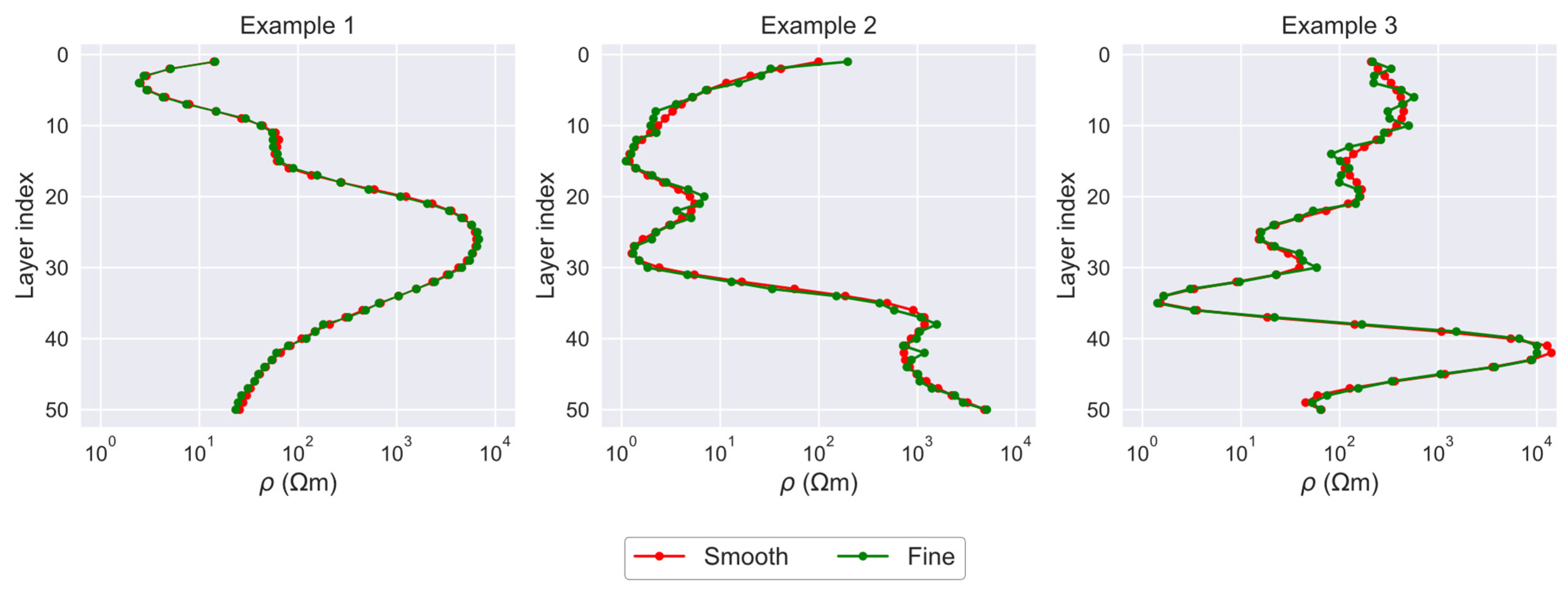
A popular method adopted by most 1D DL inversions in electromagnetic exploration is to generate a set of layered geoelectric models with smooth resistivity using spline interpolation methods. Nonetheless, the actual subsurface geoelectric structures are usually complex, and the resistivity values of layers may not be strictly smooth and gradual-changing. Hence, a novel method, that randomly adds perturbations of different amplitudes to the general smooth resistivity models is proposed to generate fine resistivity model samples that could better delineate the realistic subsurface structures. The specific steps are the following:
(a)
Select eleven layers from layer one to layer fifty evenly, and randomly assign the resistivity values ranging from 1 to 10,000 Ωm in the form of a logarithm to the eleven layers.
(b)
Calculate the resistivity values of the remaining layers by the cubic spline interpolation method, and thus obtain the smooth resistivity model ρ .
(c)
Use the following equations to add perturbations to the smooth resistivity model ρ , and thus obtain the perturbed resistivity model ρ :
{ c = 1 + ( ( ρ max / ρ min ) 1 ) ρ max ρ ρ max ρ min ρ = ρ ( 1 + 0.015 ( k 0.5 ) c )
where k with the same dimension as ρ returns random floats in the half-open interval [0, 1).
(d)
Apply 1D interpolating spline to ρ to slightly smooth the perturbations.
(e)
Replace the resistivity values outside the predetermined range with the upper and lower bounds, and finally, obtain the fine resistivity model ρ f i n e .
Figure 4 shows three representative comparison examples of the general smooth and our proposed fine resistivity models. The fine resistivity models are all evolved from the smooth resistivity models. It can be clearly seen that the proposed fine resistivity model set not only includes models that are noticeably not strictly smooth and gradual-changing but also contains models that are similar and close to the smooth models because the added perturbations are extremely small. Compared with the smooth model set, the proposed fine model set is expected to delineate the realistic subsurface geoelectric structures.
When the resistivity model set is built, the corresponding MT forward responses are then calculated with a total number of 56 frequencies ranging from 0.001 Hz to 1000 Hz. Herein, a dataset composed of 50,000 samples, of which each sample represents one response-model pair, is constructed for network training. In the DNN training stage, 40,000 samples are used as the training sets and the remaining act as the validation sets, which corresponds to an 80/20 split. The apparent resistivity and phase values derived from the MT forward responses are used as the input and the corresponding resistivity models serve as the desired output. Since the input size of the proposed 1DUResNet is 128 × 1, both the apparent resistivity and phase of 128 × 1 size are obtained by applying the linear interpolation method to the original apparent resistivity and phase of 56 × 1 size. The input and desired output data are standardized following:
{ d ˜ = d μ σ m ˜ = lg ( m )
where μ and σ denote the mean and standard deviation values on the corresponding training dataset.

3. Experiments

3.1. Comparison between the Smooth and the Fine Sample Sets

In order to examine the effectiveness of the proposed fine sample set, the DNN is trained using the general smooth and the proposed fine sets of different sizes in a fully data-driven way, and the results are evaluated using the smooth and fine test sets that are not involved in training. The Fine 1 represents the aforementioned sample set. The newly-created datasets, including Smooth 1, Smooth 2, Fine 2, smooth test set and fine test set composed of 50,000, 100,000, 100,000, 10,000 and 10,000 samples, respectively, are also built following the steps described in Section 2.4, and the fine sets are evolved from the corresponding smooth sets.
The quantitative comparison results are shown in Table 1. It can be clearly seen that the DNN trained with smooth 1 and smooth 2 performs better for the smooth test set and similarly, the DNN trained with fine 1 and fine 2 achieves better misfit results for the fine test set. When the size of training sets increases from 50,000 to 100,000, the DNN trained with a smooth set shows little improvement in model misfit for the fine test set, while the DNN trained with a fine set demonstrates a significant improvement in model misfit for the smooth test set. This means the DNN trained with the proposed fine sample set can not only deal with the earth models with gradual-changing resistivity but also make better predictions for complex subsurface structures whose resistivities appear to fluctuate. Moreover, when the size of the training set doubles, the data misfit increases rather than decreases, unlike the model misfit. This may be due to the fully data-driven DNN tending to oversmooth or overfit the model misfit, which suggests the necessity of introducing the physics to help guide the network training.

3.2. Comparison of DL Inversion Schemes with Different Drive Types

To demonstrate the validity of the proposed physics-driven DL approach (PhyDNN), this part quantitatively compares the inversion results of the test set with the fully data-driven DL approach (PlainDNN). The test set (the same is below) is a combination (20,000 samples) of the smooth and fine test sets mentioned in Section 3.1.
Figure 5 shows the convergence curves of the model and data misfits during the training process, respectively. The model and data misfits of the training and validation sets decline with epochs (one epoch means training all sample data in training sets once) gradually, indicating no overfitting phenomena. Due to the relatively large learning rate in the early training stage, the validation curves appear as a sharp jitter, which would facilitate the search for the global optimal network parameters. The comparison of the inversion results from the test set between PlainDNN and PhyDNN is shown in Figure 6. The left picture plots the model misfit scatter density. It is clear that the model misfit points are evenly distributed on both sides of the line y = x overall. As the misfit value increases, the trendline of the model misfit scatters slightly and tends to the side of PlainDNN. This indicates that PhyDNN and PlainDNN are quite comparable in model misfit, but the latter has slightly more extreme values. The right picture plots the data misfit density. The data misfit points are mainly distributed on the side of PlainDNN and the trendline obviously tends to PlainDNN, reflecting that the PhyDNN achieves a much smaller data misfit. The comparison of mean misfit values shown in Table 2 also confirms the superiority of our proposed PhyDNN.
To obtain a further understanding of the potential of the proposed PhyDNN, the anti-noise performance of PhyDNN and PlainDNN is investigated. With other conditions unchanged, the test set mixed with Gaussian noise of different levels from 0.5% to 5% is used to evaluate the well-trained PhyDNN and PlainDNN. The noise is added to the MT responses (apparent resistivity and phase). It should be noted that herein, the PhyDNN and PlainDNN are trained based on noise-free data but evaluated using noisy data. As shown in Figure 7, the difference in model misfit between PhyDNN and PlainDNN gets larger with the noise level and then tends to decrease. The difference in data misfit first becomes larger and then keeps steady as the noise level increases. The PhyDNN outperforms the PlainDNN in both model and data misfits at all noise levels. Evidently, owing to the incorporation of the physical laws of MT wave propagation, the PhyDNN is more noise-robust compared with the PlainDNN.
To analyze the effect of the two misfit terms in the loss objective function on PhyDNN inversion performance, a comparison experiment using different weighted parameter pairs ( α β ) is conducted. α and β represent the weighted parameters of model misfit term and data misfit term, respectively, which sum to 1. The weighted parameter pairs (1–0) and (0–1) denote the purely data-driven DL inversion scheme and the fully physics-based DL inversion scheme similar to the deterministic method, respectively. As clearly shown in Figure 8, the data misfit of the test set shows a downward trend when β increases from 0 to 0.7 (the corresponding α declines from 1 to 0.3). Meanwhile, the model misfit remains stable at a low level and hits the bottom when ( α β ) is (0.5–0.5). Then, as β varies from 0.7 to 0.9, the data misfit and model misfit of the test set both increase rapidly. When β reaches 1, due to the lack of the contribution of the model misfit term, though the data misfit drops to a relatively low level, the corresponding model misfit of the test set experiences a serious increase. Therefore, for balancing the two misfit terms, the reasonable β is 0.5, 0.6 and 0.7, and the corresponding α is 0.5, 0.4, and 0.3. In this work, the chosen ( α β ) is (0.5–0.5).

3.3. Comparison between the PhyDNN and the Deterministic Method

This part presents a comparative experiment between the proposed PhyDNN and the classical Occam [3] inversion methods to demonstrate the superiority of the PhyDNN over the deterministic methods. The above-mentioned test set composed of 20,000 samples is employed for inversion. Occam inversions are all performed using a number of 30 iterations and an initial model of 100 Ωm homogeneous half space and run in Matlab 2020b.
Figure 9 plots the model and data misfit scatter density between Occam and PhyDNN for the test set. It is noticeable that PhyDNN achieves a much better inversion effect than Occam for the synthetic samples in the test set. The PhyDNN is greatly superior to the Occam in both the model and data misfits, as also shown in Table 3. Table 4 exhibits the computational time of Occam and PhyDNN for inverting the test set. The Occam method requires 4.8 h on the used desktop computer to complete the inversion process for all 20,000 synthetic samples. Though the PhyDNN may be a little time-consuming in the extra stage of sample data generation and network training, it can achieve instantaneous inversion once the network is well-trained in advance, which is particularly desirable for large-scale measurements and practical for instant decision-making in fieldwork. The time consumed by PhyDNN inversion includes loading the well-trained network model and producing the network prediction.

3.4. Comparison of Different Types of MT Data

This section means to confirm the validity of the proposed multi-head DNN that uses the joint data of apparent resistivity and phase as input, by comparison with the other two input data types of individual apparent resistivity and phase. When the input data type is individual apparent resistivity or phase, the multi-head DNN that consists of two individual network paths in Figure 3 is replaced with the corresponding single-path DNN based on 1DUResNet with other conditions unchanged.
Figure 10 shows the training and validation convergence curves of PhyDNN for three types of MT data. The training and validation losses decrease with epochs progressively, and the joint data of apparent resistivity and phase performs best on both training and validation sets. Figure 11 illustrates the model and data misfit scatter density between the apparent resistivity, phase and joint data for the test set. The distribution characteristics of model and data misfit points and the trend of trendlines indicate that the joint data surpasses the other two data types in inversion effect for the test set, which coincides with the comparison result of mean model and data misfits in Table 5. Therefore, the proposed multi-head DNN can take full advantage of the subsurface information provided by the apparent resistivity and phase, and thus improve the inversion effect.

4. Examples and Results

4.1. Synthetic Data

To examine the inversion performance of the proposed PhyDNN inversion scheme, a 2D synthetic subsurface resistivity model (Figure 12a) with a length of 50 km and a depth of 10 km is designed for the inversion trial. The resistivity model has 101 sites at a distance interval of 500 m and the 1D resistivity model of each site is used to calculate the corresponding synthetic noise-free MT responses to be inverted.
Figure 12 shows the true model and the inversion results of the PlainDNN, PhyDNN and Occam methods, and Figure 13 illustrates the corresponding simulated MT responses (only the apparent resistivity is shown here). The maps are produced in the Surfer software with an application of the Kriging interpolation method [29] (the same is below). It is clear that all three methods can accurately delineate the subsurface resistivity distribution, and the corresponding simulated MT responses of the retrieved resistivity models are in great agreement with the true values. Compared with PlainDNN, PhyDNN output is overall closer to the true model and delivers more accurate resistivity values at some local depths. The same comparison results of the simulated responses between PlainDNN and PhyDNNare supported in Figure 12e and Figure 13e, where the PhyDNN has lower overall misfit and fewer extreme misfit values, particularly in data misfit. In contrast, the built DL-based inversion methods produce noticeably more accurate resistivity values than the deterministic Occam method.
To further assess the robustness and stability of the PhyDNN, the anti-noise performance of PlainDNN, PhyDNN and Occam inversion methods is evaluated using synthetic noisy data. A 2D synthetic subsurface resistivity model is redesigned in Figure 14a, and then contaminates the corresponding simulated MT responses (apparent resistivity and phase) with Gaussian noise at a 1% level. The PlainDNN and PhyDNN are all trained on the built noise-free synthetic sample dataset. As shown in Figure 14 and Figure 15, all three methods can reflect the overall distribution characteristics of the electrical properties, and the recovered simulated apparent resistivity sections agree well with the original section. However, compared with the other two methods, the PhyDNN produces more faithful and accurate inversion results in retrieving the resistivity values and delineating the shape, range and boundary of the anomaly. In contrast, the recovered resistivity from PlainDNN and Occam and the simulated apparent resistivity from PlainDNN have relatively larger deviations from the true values. Hence, owing to the incorporation of the physical laws of MT wave propagation, the proposed PhyDNN could be better at dealing with noisy measurements and yield more reliable inversion results than PlainDNN and Occam, which shows its promising prospect in practical applications.
Moreover, it can be observed in two inversion examples that though the Occam inversion method is inferior to the built DL-based inversion methods in retrieving the resistivity value, it produces accurate simulated MT responses, even more accurate than PhyDNN in the second example. This is due to the deterministic inversion methods usually employing the data misfit (or plus regularization term) as the objective function to search for the optimal solution. In addition, it is demonstrated that the proposed PhyDNN inversion method is quite robust, as it accurately recovers the lateral coherence of the resistivity section, though the resistivity models of all sites are inverted individually.

4.2. Field Data

To verify the applicability of the proposed PhyDNN inversion scheme to field measurements, the MT data sets collected in South Australia, Australia by Adelaide University, which are publicly available from Krieger and Peacock [28], are employed for inversion. As shown in Figure 16, a total of 15 sites were recorded with a frequency range of 0.0046 Hz to 78 Hz. The topography of the survey area is quite flat and varies from 22 m to 56 m along the survey line.
A phase tensor analysis of the field measurements is performed and the results are illustrated in Figure 17. In Figure 17a, the ellipses are colored according to the minimum phase tensor value ϕ min [30]. It is clear that the phase tensors can be divided into three parts with frequency decreasing. In the frequency range of 78 Hz to 1 Hz, ϕ min is mostly larger than 45°, which means there exist conductive layers near the surface. For the frequency of 1 Hz to 0.1 Hz, ϕ min is much lower than 45°, indicating the existence of highly resistive layers at the corresponding depths. For the frequency of 0.1 Hz to 0.0046 Hz, ϕ min is slightly higher than 45°, suggesting there follows a relatively conductive zone. Figure 17b illustrates the phase tensor ellipses colored by the skew angle [30,31]. For frequencies higher than 1 Hz, the skew angles of phase tensor ellipses are mostly less than 3 in absolute value, meaning the resistivity structure near the surface tends to be 1D. The rest phase tensor ellipses with larger absolute values of skew angle suggest that the resistivity structure of the relatively deeper zone is more likely to be 2D or 3D.
Following the steps in Section 2.4, the training sets composed of 50,000 samples are regenerated using the same configurations of synthetic resistivity models and resistivity values range but a different frequency band of 0.0046 Hz to 78 Hz. Then the PhyDNN is retained and the well-trained network is applied to produce predictions. This work also benchmarks it against the classical Occam inversion method using a number of 30 iterations and an initial model of 100 Ωm homogeneous half space. As shown in Figure 18, the 2D pseudo section maps along the survey profile are generated by stitching the 1D inversion results or the corresponding MT responses together. Figure 19 shows the data misfit of each individual site and the overall data misfit for all sites. It can be clearly seen that the inversion results of the two methods are quite compatible and show synchronous changes, and the corresponding apparent resistivity values also agree well with the real measurements. The inverted resistivity models overall present a low-high-low resistivity change trend with increasing depth. The resistivity structure near the subsurface tends to be 1D, whereas that at the deeper depth is more likely to be 2D or 3D. These findings coincide with the phase tensor analysis results.

5. Discussion and Conclusions

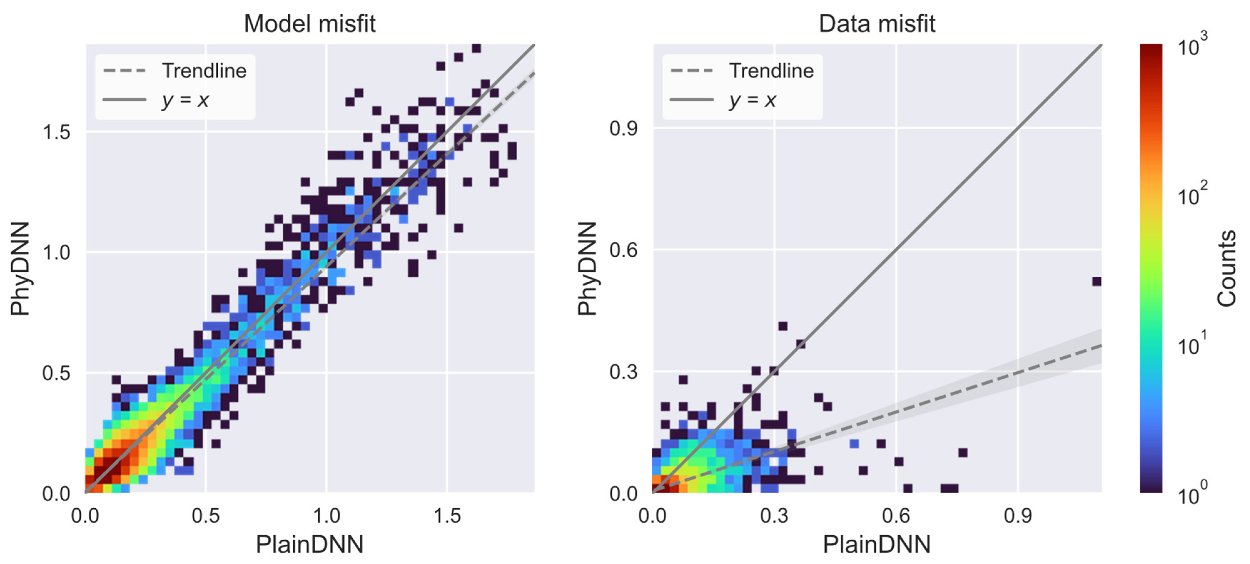
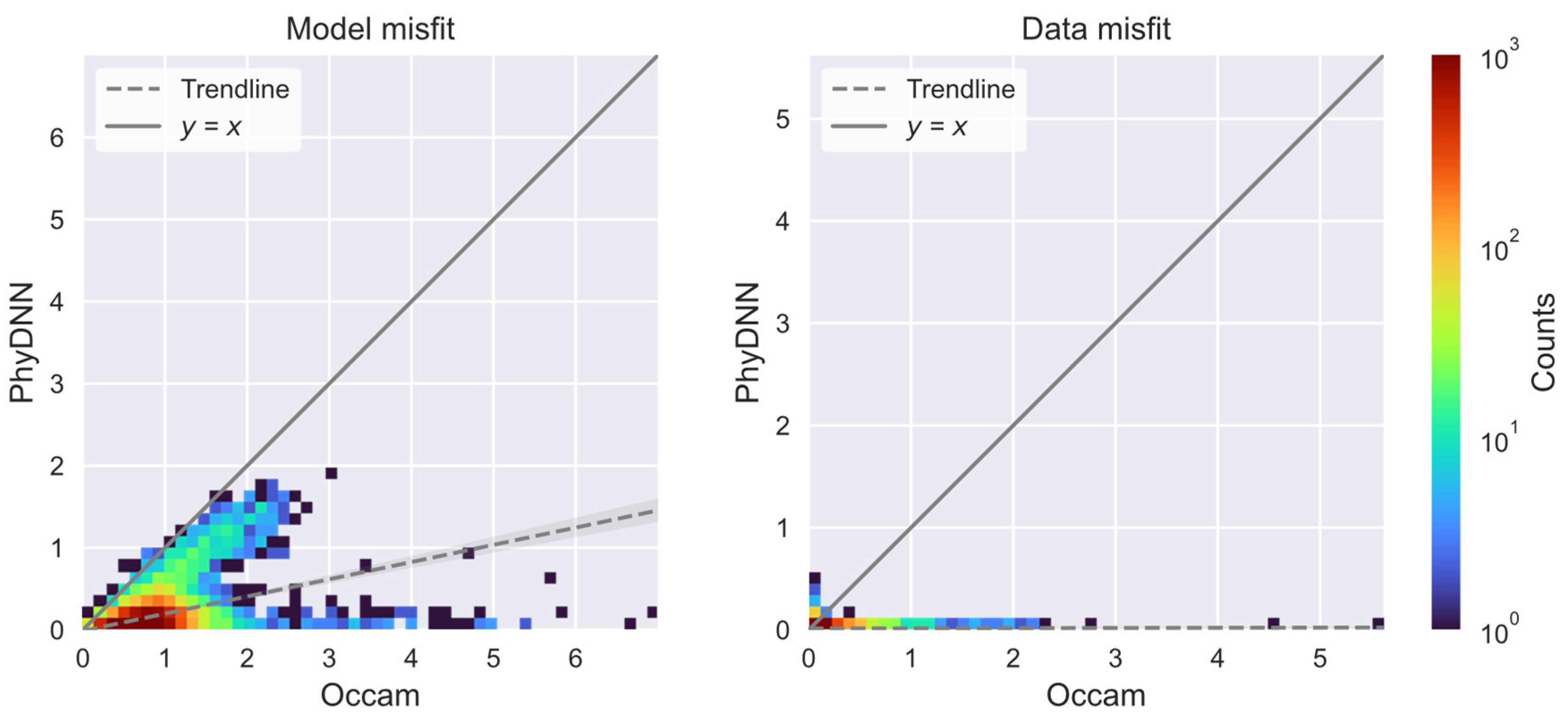
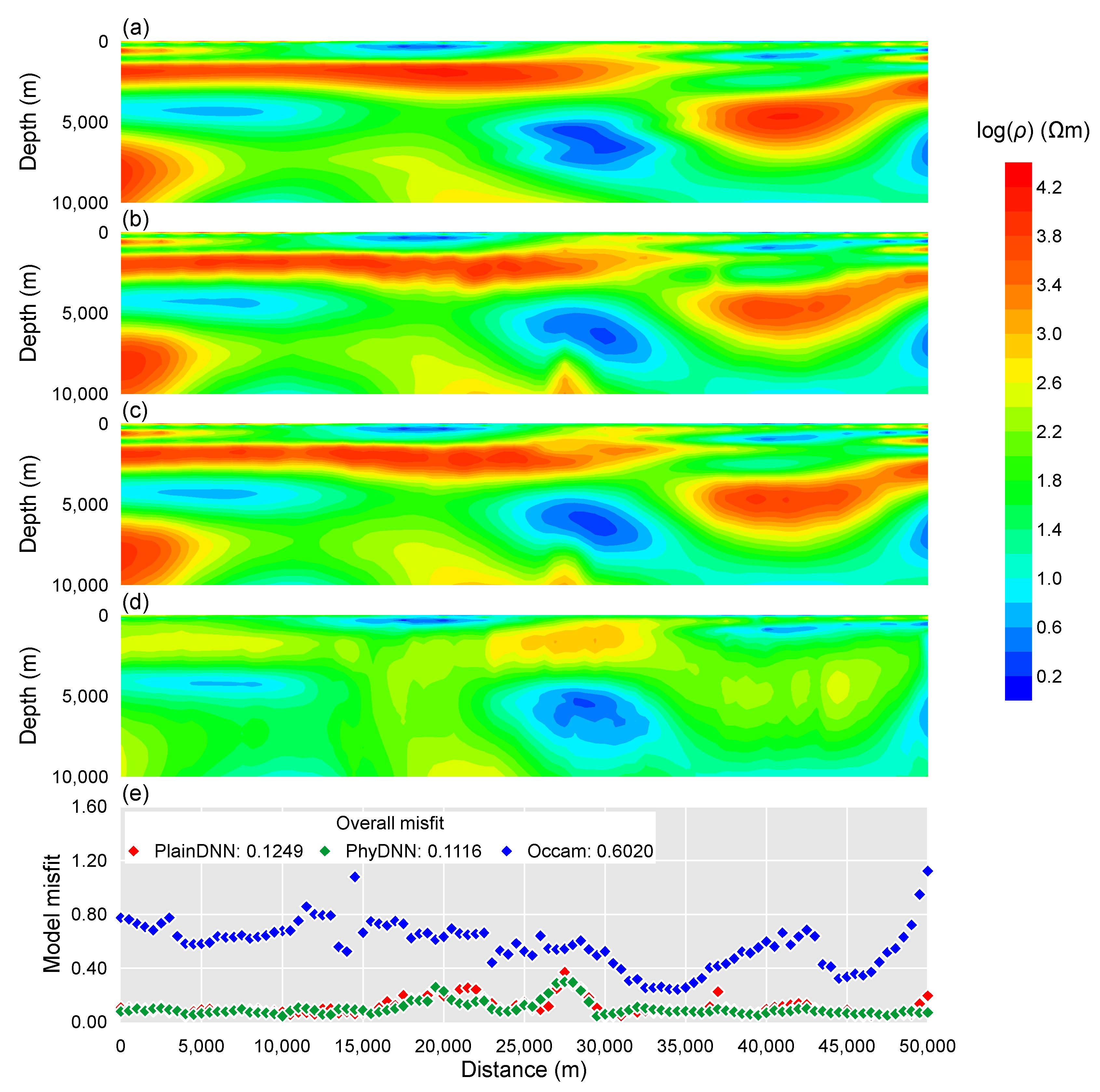
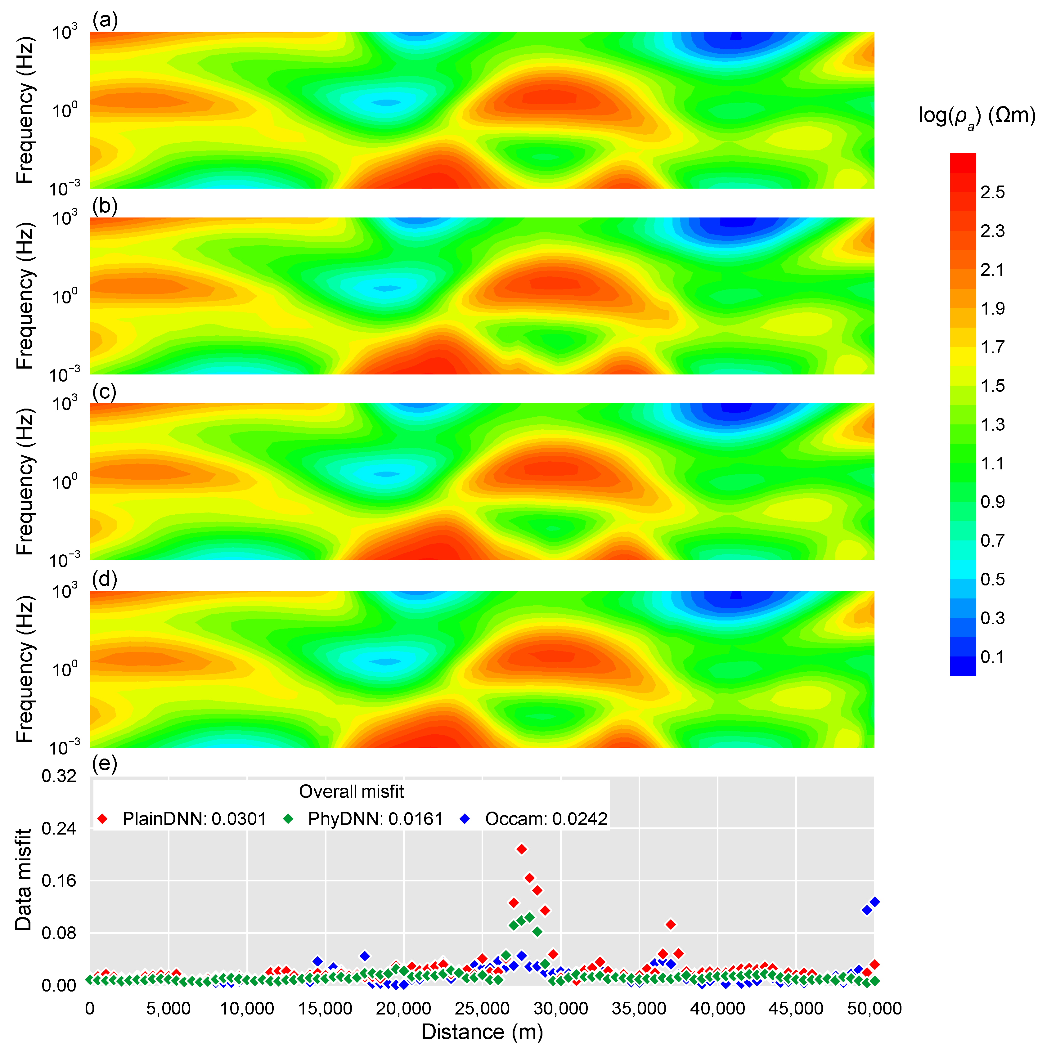
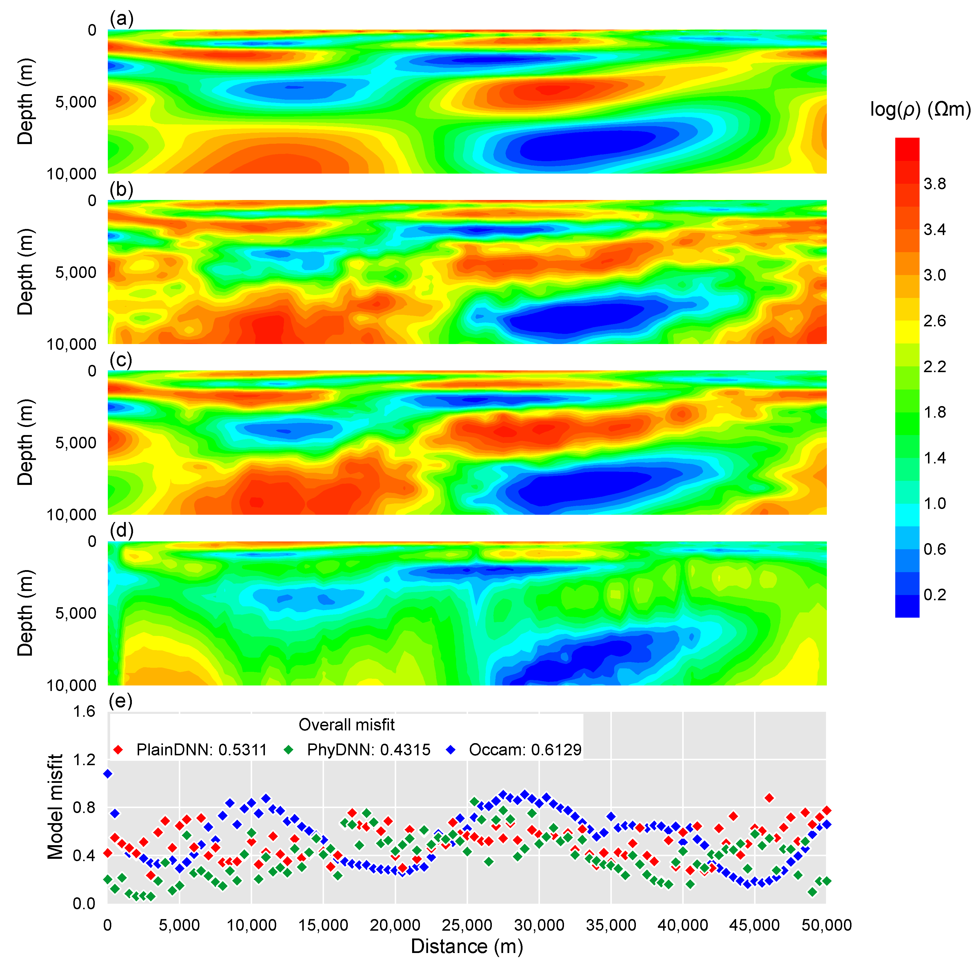
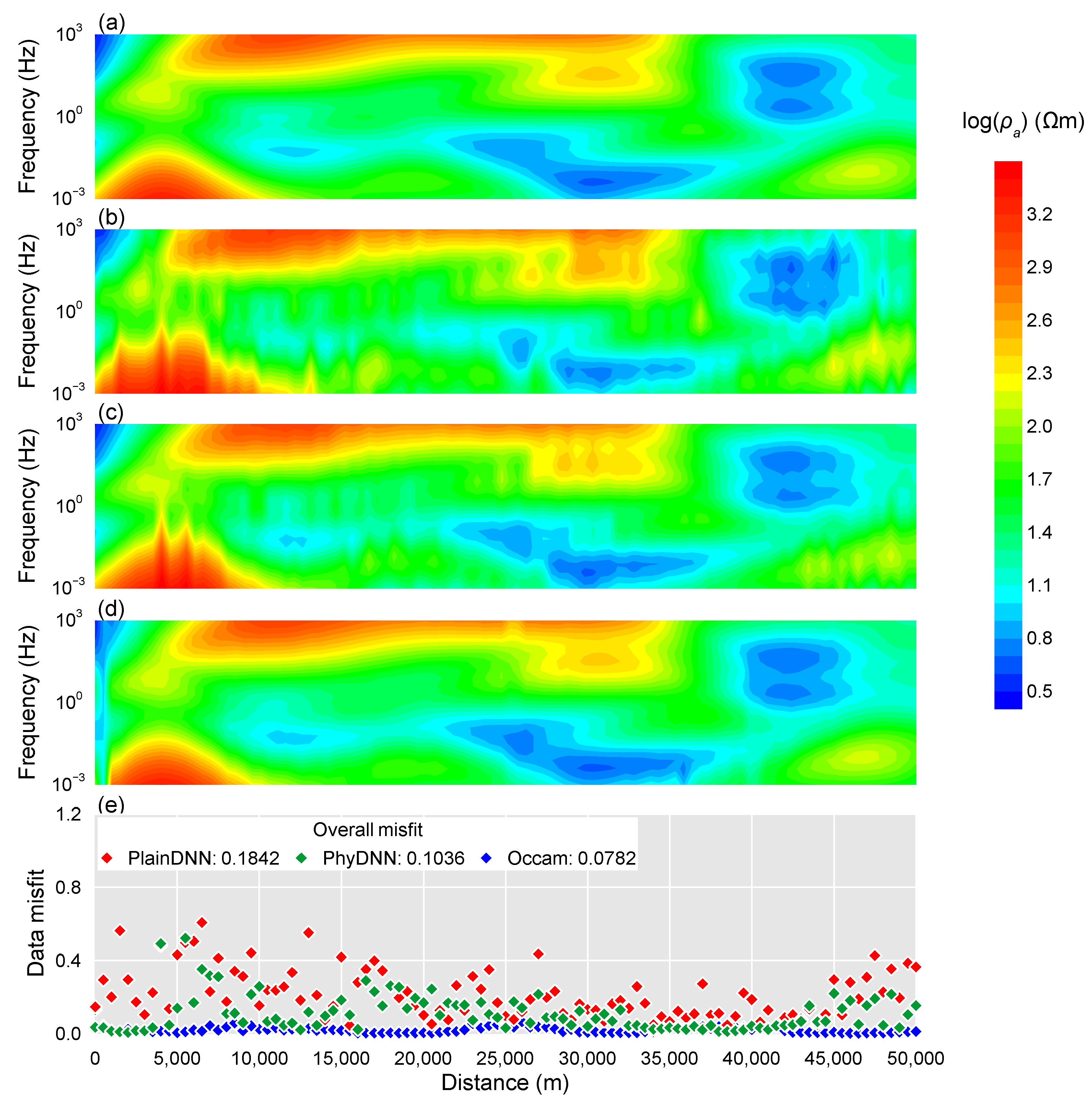
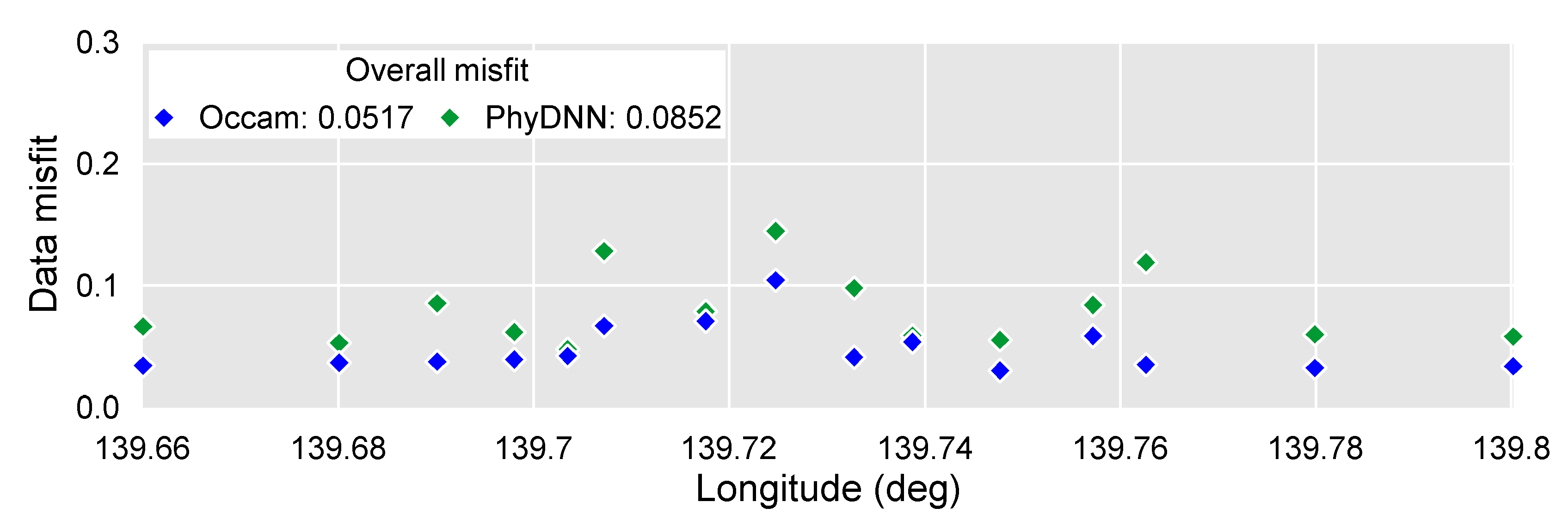
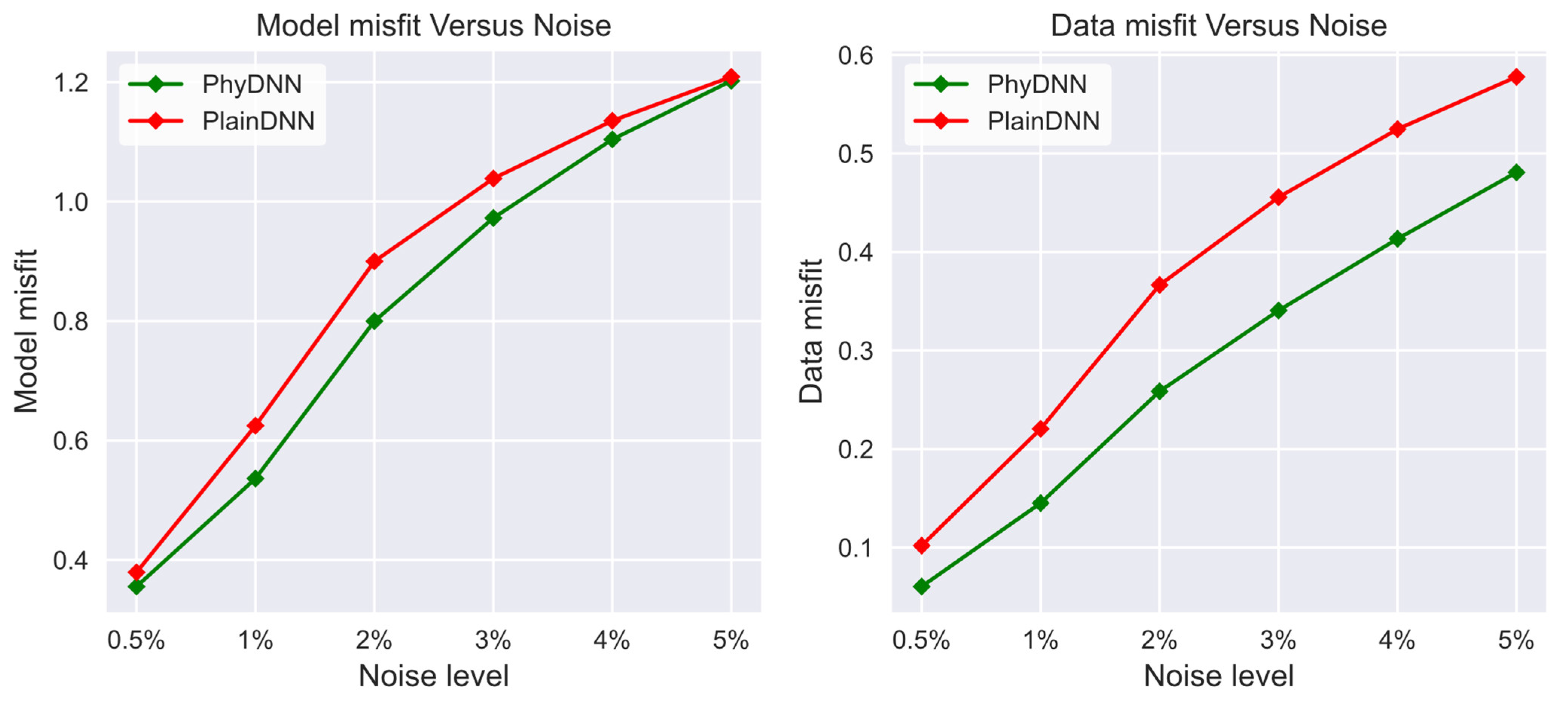
This work proposes a novel physics-driven DL-based MT inversion method (named PhyDNN), which embeds the forward operator modeling MT wave propagation into the network architecture in the form of using the weighted sum of model misfit m and physics-based data misfit d as the loss objective function to guide the network training. Consequently, the proposed PhyDNN can take advantage of the fully data-driven DL and deterministic methods, thus reducing the dependency on extensive training sets and having the ability to deal with complex realistic exploration scenarios. It is demonstrated that the PhyDNN can honor the physical laws of the MT inverse problem and accurately reconstruct the nonlinear mapping from the input (apparent resistivity and phase) to the output (resistivity model). Quantitative and qualitative analysis results show that the PhyDNN inversion outperforms the PlainDNN inversion in model misfit and particularly in physics-based data misfit and that the former is more robust and can yield more reliable inversion results when dealing with noisy measurements. Compared with the classical deterministic Occam inversion method, the built DL-based inversion methods, particularly the proposed PhyDNN, perform better in retrieving the resistivity values and delineating the resistivity distribution. To further verify the feasibility and applicability of PhyDNN, a comparison inversion for field data between the PhyDNN and Occam methods is implemented. The PhyDNN inversion results are quite compatible with the Occam method, and the corresponding simulated MT responses are in good agreement with the actual measurements. Moreover, compared with the conventional deterministic method, the DL-based method can realize instantaneous inversion without any iterations once the network is well-trained in advance, which is particularly desirable for large-scale measurements and practical for instant decision-making in fieldwork. In addition, the fine resistivity models generated by the proposed novel method could better delineate the real-world subsurface structure compared to the commonly-used smooth resistivity models, which facilitates the DL inversion for complex subsurface structures whose resistivities appear to fluctuate. This model construction method could be applied to other existing geophysical techniques for solving 1D inverse problems.
The proposed physics-driven DL inversion strategy can be extended to 2D and 3D MT inverse problems. However, unless sufficient computational power is available, it is extremely difficult or impossible to perform T (the number of samples involved in training) times 2D (or 3D) MT forwarding in every training loop. Hence, how to reasonably introduce the 2D (or 3D) forward operator simulating the MT wave propagation into the network architecture to improve MT inversion is a challenging problem and will be our future work.

Author Contributions

Conceptualization, W.L. and Z.X.; methodology, W.L. and H.W.; validation, W.L., Z.X., H.W., R.Z. and X.H.; formal analysis, W.L.; investigation, W.L.; resources, W.L., Z.X., H.W., R.Z. and X.H.; data curation, W.L.; writing—original draft preparation, W.L.; writing—review and editing, W.L.; visualization, W.L.; supervision, W.L. and H.W.; project administration, W.L. and H.W.; funding acquisition, Z.X. All authors have read and agreed to the published version of the manuscript.

Funding

This research was funded by the National Natural Science Foundation of China (No. 41304090), the National Key Research and Development Project of China (No. 2016YFC0303104), and the Ocean 13th Five-Year International Marine Resources Survey and Development of China (No. DY135-S1-1-07).

Data Availability Statement

Not applicable.

Acknowledgments

We thank the three anonymous reviewers and editors for their constructive comments on the original manuscript. We also thank Krieger and Peacock for providing the MT field data in South Australia, Australia.

Conflicts of Interest

The authors declare no conflict of interest.

References

  1. Tikhonov, A.N. Determination of the electrical characteristics of the deep strata of the earth’s crust. Dolk. Acad. Nauk. SSSR 1950, 73, 295–311. [Google Scholar]
  2. Cagniard, L. Basic Theory of the Magnetotelluric Method of Geophysical Prospecting. Geophysics 1953, 18, 605–635. [Google Scholar] [CrossRef]
  3. Constable, S.C.; Parker, R.L.; Constable, C.G. Occam’s inversion: A practical algorithm for generating smooth models from electromagnetic sounding data. Geophysics 1987, 52, 289–300. [Google Scholar] [CrossRef]
  4. Siripunvaraporn, W.; Egbert, G. An efficient data-subspace inversion method for 2-D magnetotelluric data. Geophysics 2000, 65, 791–803. [Google Scholar] [CrossRef]
  5. Newman, G.A.; Alumbaugh, D.L. Three-dimensional magnetotelluric inversion using non-linear conjugate gradients. Geophys. J. Int. 2002, 140, 410–424. [Google Scholar] [CrossRef] [Green Version]
  6. Kelbert, A.; Egbert, G.D.; Schultz, A. Non-linear conjugate gradient inversion for global EM induction: Resolution studies. Geophys. J. Int. 2008, 173, 365–381. [Google Scholar] [CrossRef]
  7. Grayver, A.V.; Streich, R.; Ritter, O. Three-dimensional parallel distributed inversion of CSEM data using a direct forward solver. Geophys. J. Int. 2013, 193, 1432–1446. [Google Scholar] [CrossRef] [Green Version]
  8. Liu, Y.; Yin, C.C. 3D inversion for multipulse airborne transient electromagnetic data. Geophysics 2016, 81, E401–E408. [Google Scholar] [CrossRef]
  9. Blatter, D.; Key, K.; Ray, A.; Foley, N.; Tulaczyk, S.; Auken, E. Trans-dimensional Bayesian inversion of airborne transient EM data from Taylor Glacier, Antarctica. Geophys. J. Int. 2018, 214, 1919–1936. [Google Scholar] [CrossRef]
  10. Guo, R.W.; Dosso, S.E.; Liu, J.X.; Dettmer, J.; Tong, X.Z. Non-linearity in Bayesian 1–D magnetotelluric inversion. Geophys. J. Int. 2011, 185, 663–675. [Google Scholar] [CrossRef] [Green Version]
  11. Wang, H.; Liu, M.L.; Xi, Z.Z.; Peng, X.L.; He, H. Magnetotelluric inversion based on BP neural network optimized by genetic algorithm. Chin. J. Geophys. 2018, 61, 1563–1575. [Google Scholar]
  12. Araya-Polo, M.; Jennings, J.; Adler, A.; Dahlke, T. Deep-learning tomography. Lead. Edge 2018, 37, 58–66. [Google Scholar] [CrossRef]
  13. Das, V.; Pollack, A.; Wollner, U.; Mukerji, T. Convolutional neural network for seismic impedance inversion. Geophysics 2019, 84, R869–R880. [Google Scholar] [CrossRef]
  14. Puzyrev, V. Deep learning electromagnetic inversion with convolutional neural networks. Geophys. J. Int. 2019, 218, 817–832. [Google Scholar] [CrossRef] [Green Version]
  15. Bai, P.; Vignoli, G.; Viezzoli, A.; Nevalainen, J.; Vacca, G. (Quasi-) Real-Time Inversion of Airborne Time-Domain Electromagnetic Data via Artificial Neural Network. Remote Sens. 2020, 12, 3440. [Google Scholar] [CrossRef]
  16. Wu, S.H.; Huang, Q.H.; Zhao, L. Convolutional neural network inversion of airborne transient electromagnetic data. Geophys. Prospect. 2021, 69, 1761–1772. [Google Scholar] [CrossRef]
  17. Wang, H.; Liu, W.; Xi, Z.Z. Nonlinear inversion for magnetotelluric sounding based on deep belief network. J. Cent. South Univ. 2019, 26, 2482–2494. [Google Scholar] [CrossRef]
  18. Liu, Z.G.; Chen, H.; Ren, Z.Y.; Tang, J.T.; Xu, Z.M.; Chen, Y.P.; Liu, X. Deep learning audio magnetotellurics inversion using residual-based deep convolution neural network. J. Appl. Geophys. 2021, 188, 104309. [Google Scholar] [CrossRef]
  19. Adler, J.; Öktem, O. Solving ill-posed inverse problems using iterative deep neural networks. Inverse Probl. 2017, 33, 124007. [Google Scholar] [CrossRef] [Green Version]
  20. Raissi, M.; Perdikaris, P.; Karniadakisa, G.E. Physics-informed neural networks: A deep learning framework for solving forward and inverse problems involving nonlinear partial differential equations. J. Comput. Phys. 2019, 378, 686–707. [Google Scholar] [CrossRef]
  21. Fuks, O.; Tchelepi, H.A. Limitations of physics informed machine learning for nonlinear two-phase transport in porous media. J. Mach. Learn. Model. Comput. 2020, 1, 19–37. [Google Scholar] [CrossRef]
  22. Colombo, D.; Turkoglu, E.; Li, W.; Sandoval-Curiel, E.; Rovetta, D. Physics-driven deep-learning inversion with application to transient electromagnetics. Geophysics 2021, 86, E209–E224. [Google Scholar] [CrossRef]
  23. Sun, J.; Niu, Z.; Innanen, K.A.; Li, J.; Trad, D.O. A theory-guided deep-learning formulation and optimization of seismic waveform inversion. Geophysics 2020, 85, R87–R99. [Google Scholar] [CrossRef]
  24. Wang, Y.; Wang, Q.; Lu, W.; Li, H. Physics-constrained seismic impedance inversion based on deep learning. IEEE Geosci. Remote Sens. Lett. 2021, 19, 1–5. [Google Scholar] [CrossRef]
  25. Ronneberger, O.; Fischer, P.; Brox, T. U-net: Convolutional networks for biomedical image segmentation. In Proceedings of the Medical Image Computing and Computer-Assisted Intervention-MICCAI 2015, Munich, Germany, 5–9 October 2015. [Google Scholar]
  26. He, K.; Zhang, X.; Ren, S.; Sun, J. Deep residual learning for image recognition. In Proceedings of the IEEE Conference on Computer Vision and Pattern Recognition, Las Vegas, NV, USA, 26 June–1 July 2016. [Google Scholar]
  27. Long, J.; Shelhamer, E.; Darrell, T. Fully convolutional networks for semantic segmentation. IEEE Trans. Pattern Anal. Mach. Intell. 2014, 39, 640–651. [Google Scholar]
  28. Krieger, L.; Peacock, J.R. MTpy: A Python Toolbox for Magnetotellurics. Comput. Geosci. 2014, 72, 167–175. [Google Scholar] [CrossRef]
  29. Chen, H.H.; Li, X.; Ding, W.X. Twelve kinds of Gridding Methods of Surfer 8.0 in isoline drawing. Chin. J. Eng. Geophys. 2007, 4, 52–57. [Google Scholar]
  30. Caldwell, T.G.; Bibby, H.M.; Brown, C. The magnetotelluric phase tensor. Geophys. Geophys. J. Int. 2004, 158, 457–469. [Google Scholar] [CrossRef] [Green Version]
  31. Bibby, H.M.; Caldwell, T.G.; Brown, C. Determinable and non-determinable parameters of galvanic distortion in magnetotellurics. Geophys. J. Int. 2005, 163, 915–930. [Google Scholar] [CrossRef]
Figure 1. High-level illustration of the forward and inverse problems.
Remotesensing 14 03218 g001
Figure 2. Architecture of the proposed 1DUResNet following Unet-like and ResNet-like 1D CNN design.
Remotesensing 14 03218 g002
Figure 3. An overview of the proposed physics−driven DL (PhyDNN) inversion scheme for MT.
Remotesensing 14 03218 g003
Figure 4. Three representative examples of comparison between the general smooth and the proposed fine resistivity models. The fine resistivity models are evolved from the smooth resistivity models.
Remotesensing 14 03218 g004
Figure 5. The model and data misfit convergence curves of the training and validation sets in the training process from the PlainDNN and PhyDNN.
Remotesensing 14 03218 g005
Figure 6. The model and data misfit scatter density plots between the PlainDNN and PhyDNN for the test set.
Remotesensing 14 03218 g006
Figure 7. Comparison of the anti-noise performance between PhyDNN and PlainDNN at different levels of Gaussian noise. The left is the mean model misfit of the test set from PhyDNN and PlainDNN, and the right presents the mean data misfit of the test set from PhyDNN and PlainDNN.
Remotesensing 14 03218 g007
Figure 8. Comparison of the effect of different weighted parameter pairs ( α β ) on PhyDNN inversion. α and β denote the weighted parameters of model misfit term and data misfit term, respectively, which sum to 1. The left and right y-axes plot the model misfit and data misfit separately.
Remotesensing 14 03218 g008
Figure 9. The model and data misfit scatter density plots between the Occam and PhyDNN for the test set.
Remotesensing 14 03218 g009
Figure 10. The training and validation convergence curves of PhyDNN for the apparent resistivity, phase and joint data.
Remotesensing 14 03218 g010
Figure 11. The model and data misfit scatter density plots between the apparent resistivity, phase and joint data for the test set. The left and right columns are the comparison results of model misfit and data misfit separately. The top row places the comparison results between the apparent resistivity and joint data. The bottom row shows the comparison results between the phase and joint data.
Remotesensing 14 03218 g011
Figure 12. Comparison of the inversion results of the PlainDNN, PhyDNN and Occam methods. (ad) are the true model, the recovered models of the PlainDNN, PhyDNN and Occam, respectively. (e) shows the individual model misfit for all sites and the overall model misfit of the whole model.
Remotesensing 14 03218 g012
Figure 13. Comparison of the corresponding simulated apparent resistivity sections of the models shown in Figure 12. (ad) are the real apparent resistivity, the simulated apparent resistivity of the PlainDNN, PhyDNN and Occam, respectively. (e) shows the individual data misfit for all sites and the overall data misfit of the whole model.
Remotesensing 14 03218 g013
Figure 14. Comparison of the inversion results for subsurface resistivity model (ad) are the retrieved models of the PlainDNN, PhyDNN and Occam, respectively. (e) shows the individual model misfit for all sites and the overall model misfit of the whole model. The MT responses used for inversion are mixed with Gaussian noise at 1% level.
Remotesensing 14 03218 g014
Figure 15. Comparison of the corresponding simulated apparent resistivity sections of the models shown in Figure 14. (a–d) are the real apparent resistivity, the simulated apparent resistivity of the PlainDNN, PhyDNN and Occam, respectively. (e) shows the individual data misfit for all sites and the overall data misfit of the whole model.
Remotesensing 14 03218 g015
Figure 16. Field map of the MT survey line in South Australia, Australia. The black triangles represent the MT stations collecting the surface measurements. The box on the top-left and the red star denote the worldwide location of the MT exploration project.
Remotesensing 14 03218 g016
Figure 17. Pseudosection plots of phase tensor ellipses along the measurement profile. The ellipses in (a,b) are normalized by the maximum phase value and colored according to the minimum phase tensor value ϕ min or skew angle.
Remotesensing 14 03218 g017
Figure 18. The inversion results and the corresponding MT responses of filed data. (a) shows the elevation section along the survey profile. (b,c) are the pseudo cross-sections of the inverted resistivity models recovered by the Occam and PhyDNN methods, respectively. (df) show the real responses and the corresponding simulated responses (only the apparent resistivity is shown here) of the inversion results for the Occam and PhyDNN methods separately.
Remotesensing 14 03218 g018
Figure 19. The data misfit of each individual site and the overall data misfit for all sites.
Remotesensing 14 03218 g019
Table 1. Mean model and data misfits of test sets for the general smooth and the proposed fine sample sets.
Training SetSmooth Test SetFine Test Set
Model MisfitData MisfitModel MisfitData Misfit
Smooth 10.10950.02050.34610.0867
Fine 10.12320.02780.29790.0516
Smooth 20.08620.04050.34340.1102
Fine 20.10060.03380.27840.0492
Table 2. Mean model and data misfits of the test set for the PlainDNN and PhyDNN.
DL Inversion SchemeModel MisfitData Misfit
PlainDNN0.22800.0415
PhyDNN0.22260.0215
Table 3. Mean model and data misfits of the test set for Occam and PhyDNN.
Inversion MethodModel MisfitData Misfit
Occam0.84050.1928
PhyDNN0.22260.0215
Table 4. Computational loads of the Occam and PhyDNN for inverting the test set.
Inversion MethodData Generation (Hour)Training (Hour)Inversion (Hour)
Occam--4.8
PhyDNN1.2521.80.01
Table 5. Mean model and data misfits of the test set for the apparent resistivity, phase and joint data.
MT DataModel MisfitData Misfit
Phase0.26570.0541
Apparent resistivity0.23710.0265
Joint data0.22260.0215
Publisher’s Note: MDPI stays neutral with regard to jurisdictional claims in published maps and institutional affiliations.

