
Large-Scale Debris Cover Glacier Mapping Using Multisource Object-Based Image Analysis Approach

 , ,
, ,
Abstract
1. Introduction
2. Research Areas and Datasets
2.1. Research Areas
2.2. Datasets
3. Methodology
3.1. Descriptive Analysis of Glacier Cover Classes
3.1.1. Visual Interpretation
3.1.2. Spectral Analysis
3.2. Image Segmentation and Attributes Selection
3.2.1. Selecting Optimal Segmentation Parameters
3.2.2. Selection of Attributes
3.3. Multisource OBIA Classification
3.3.1. Mapping of Objects at L200 Level
3.3.2. Mapping of Objects at L60 Level
3.4. Refinement
3.5. Accuracy Assessment
4. Transferability of Proposed Multisource OBIA Approach
4.1. Same Study Area, Different Sensor Data
LISS-4 + Ancillary Dataset Analysis
4.2. Same Sensor Data, Different Study Area
5. Results
5.1. Analysis of Spectral and Spatial Properties
5.2. Comparison between the Segmentation Results without and with Ancillary Data
5.3. Assessment of Individual Class Accuracies
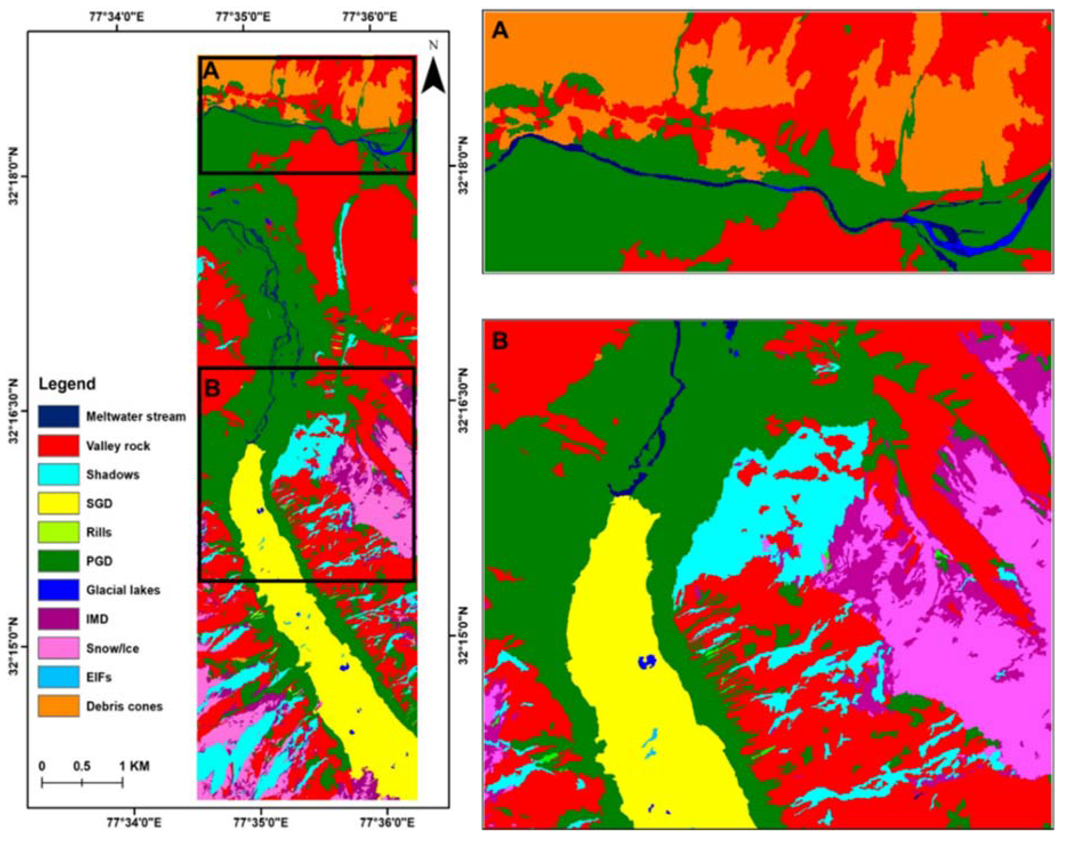
5.3.1. Gangotri Glacier
- WorldView-2 + Ancillary Dataset
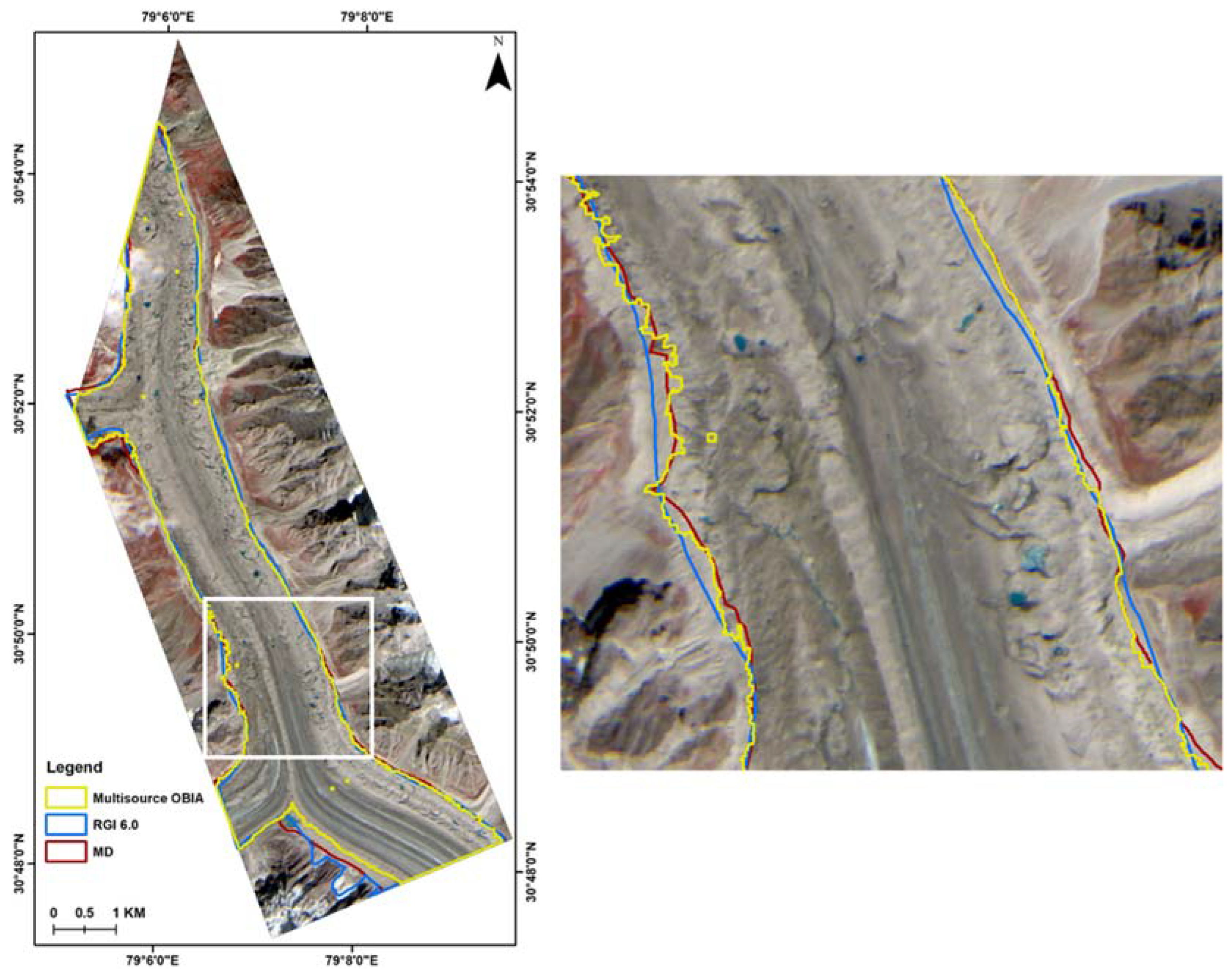
- LISS-4 + Ancillary Dataset
5.3.2. Bara Shigri Glacier
6. Discussion
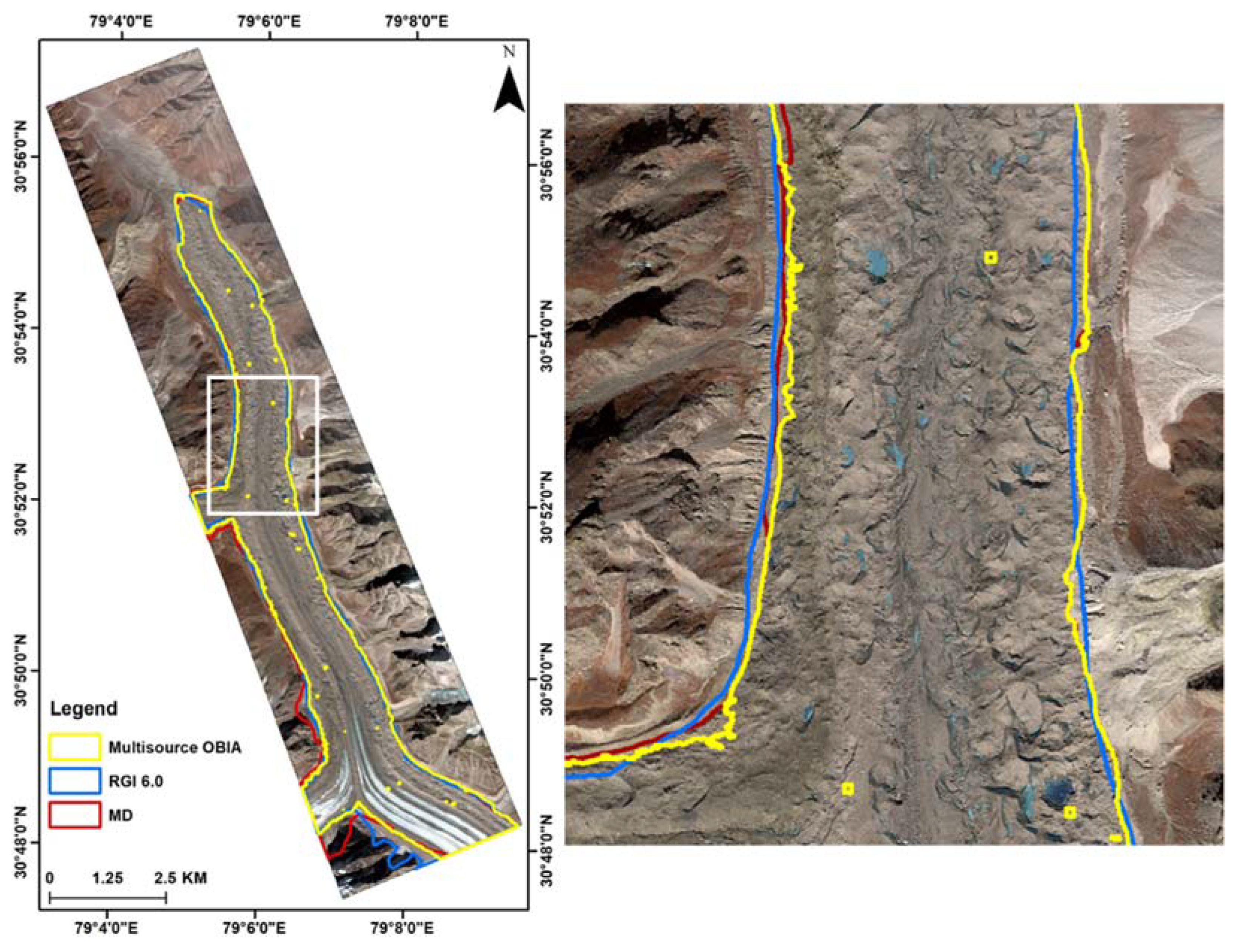
6.1. Appreciation of Glacier Boundaries
6.1.1. Gangotri Glacier
- WorldView-2 + Ancillary Dataset
- LISS-4 + Ancillary Dataset
6.1.2. Bara Shigri Glacier
6.2. Comparison with Other Debris-Covered Glacier Mapping OBIA Methods
6.3. Constraints and Potentials
7. Conclusions
Author Contributions
Funding
Data Availability Statement
Acknowledgments
Conflicts of Interest
References
- Paul, F.; Barrand, N.E.; Baumann, S.; Berthier, E.; Bolch, T.; Casey, K.; Frey, H.; Joshi, S.P.; Konovalov, V.; Le Bris, R.; et al. On the Accuracy of Glacier Outlines Derived from Remote-Sensing Data. Ann. Glaciol. 2013, 54, 171–182. [Google Scholar] [CrossRef]
- Shukla, A.; Ali, I. A Hierarchical Knowledge-Based Classification for Glacier Terrain Mapping: A Case Study from Kolahoi Glacier, Kashmir Himalaya. Ann. Glaciol. 2016, 57, 1–10. [Google Scholar] [CrossRef]
- Shugar, D.H.; Burr, A.; Haritashya, U.K.; Kargel, J.S.; Watson, C.S.; Kennedy, M.C.; Bevington, A.R.; Betts, R.A.; Harrison, S.; Strattman, K. Rapid Worldwide Growth of Glacial Lakes since 1990. Nat. Clim. Chang. 2020, 10, 1–7. [Google Scholar] [CrossRef]
- Bhambri, R.; Bolch, T. Glacier Mapping: A Review with Special Reference to the Indian Himalayas. Prog. Phys. Geogr. Earth Environ. 2009, 33, 672–704. [Google Scholar] [CrossRef]
- Xie, F.; Liu, S.; Wu, K.; Zhu, Y.; Gao, Y.; Qi, M.; Duan, S.; Saifullah, M.; Tahir, A.A. Upward Expansion of Supra-Glacial Debris Cover in the Hunza Valley, Karakoram, During 1990∼2019. Front. Earth Sci. 2020, 8, 308. [Google Scholar] [CrossRef]
- Yousuf, B.; Shukla, A.; Arora, M.K.; Jasrotia, A.S. Glacier Facies Characterization Using Optical Satellite Data: Impacts of Radiometric Resolution, Seasonality, and Surface Morphology. Prog. Phys. Geogr. Earth Environ. 2019, 43, 473–495. [Google Scholar] [CrossRef]
- Shukla, A.; Yousuf, B. Evaluation of Multisource Data for Glacier Terrain Mapping: A Neural Net Approach. Geocarto Int. 2017, 32, 569–587. [Google Scholar] [CrossRef]
- Bhardwaj, A.; Joshi, P.; Snehmani; Sam, L.; Singh, M.K.; Singh, S.; Kumar, R. Applicability of Landsat 8 Data for Characterizing Glacier Facies and Supraglacial Debris. Int. J. Appl. Earth Obs. Geoinf. 2015, 38, 51–64. [Google Scholar] [CrossRef]
- Blaschke, T. Object Based Image Analysis for Remote Sensing. ISPRS J. Photogramm. Remote Sens. 2010, 65, 2–16. [Google Scholar] [CrossRef]
- Höfle, B. Glacier Surface Segmentation Using Airborne Laser Scanning Point Cloud and Intensity Data. Int. Arch. Photogramm. Remote Sens. Spat. Inf. Sci. 2007, XXXVI, 195–200. [Google Scholar]
- Williams, M.W. The Status of Glaciers in the Hindu Kush–Himalayan Region. Mt. Res. Dev. 2013, 33, 114–115. [Google Scholar] [CrossRef]
- Rastner, P.; Bolch, T.; Notarnicola, C.; Paul, F. A Comparison of Pixel-and Object-Based Glacier Classification With Optical Satellite Images. IEEE J. Sel. Top. Appl. Earth Obs. Remote Sens. 2014, 7, 853–862. [Google Scholar] [CrossRef]
- Kraaijenbrink, P.D.A.; Shea, J.M.; Pellicciotti, F.; Jong, S.M.d.; Immerzeel, W.W. Object-Based Analysis of Unmanned Aerial Vehicle Imagery to Map and Characterise Surface Features on a Debris-Covered Glacier. Remote Sens. Environ. 2016, 186, 581–595. [Google Scholar] [CrossRef]
- Jawak, S.D.; Jadhav, A.; Luis, A.J. Object-Oriented Feature Extraction Approach for Mapping Supraglacial Debris in Schirmacher Oasis Using Very High-Resolution Satellite Data. In Proceedings of the SPIE 9877, Land Surface and Cryosphere Remote Sensing III, New Delhi, India, 5 May 2016; p. 98772L. [Google Scholar] [CrossRef]
- Sharda, S.; Srivastava, M. Classification of Siachen Glacier Using Object-Based Image Analysis. In Proceedings of the 2018 International Conference on Intelligent Circuits and Systems (ICICS), Phagwara, India, 19–20 April 2018. [Google Scholar]
- Ahmad, F.; Baig, M.H.A. Mapping of Debris-Covered Glaciers in Astor Basin: An Object-Based Image Analysis Approach. In Proceedings of the SPIE 10777, Land Surface and Cryosphere Remote Sensing IV, Honolulu, HI, USA, 16 November 2018; p. 1077704. [Google Scholar] [CrossRef]
- Thanki, D.; Israni, D.; Makwana, A. Glacier Mapping with Object Based Image Analysis Method, Case Study of Mount Everest Region. J. Kejuruter. 2019, 31, 215–220. [Google Scholar] [CrossRef]
- Robson, B.A.; Nuth, C.; Dahl, S.O.; Hölbling, D.; Strozzi, T.; Nielsen, P.R. Automated Classification of Debris-Covered Glaciers Combining Optical, SAR and Topographic Data in an Object-Based Environment. Remote Sens. Environ. 2015, 170, 372–387. [Google Scholar] [CrossRef]
- Mitkari, K.V.; Arora, M.K.; Tiwari, R.K. Extraction of Glacial Lakes in Gangotri Glacier Using Object-Based Image Analysis. IEEE J. Sel. Top. Appl. Earth Obs. Remote Sens. 2017, 10, 5275–5283. [Google Scholar] [CrossRef]
- Jawak, S.D.; Wankhede, S.F.; Luis, A.J. Exploration of Glacier Surface FaciesMapping Techniques Using Very High Resolution Worldview-2 Satellite Data. Multidiscip. Digit. Publ. Inst. Proc. 2018, 2, 339. [Google Scholar] [CrossRef]
- Jawak, S.D.; Wankhede, S.F.; Luis, A.J. Explorative Study on Mapping Surface Facies of Selected Glaciers from Chandra Basin, Himalaya Using WorldView-2 Data. Remote Sens. 2019, 11, 1207. [Google Scholar] [CrossRef]
- Bolch, T.; Kamp, U. Glacier Mapping in High Mountains Using DEMs, Landsat and ASTER Data. In Proceedings of the 8th International Symposium on High Mountain Remote Sensing Cartography, La Paz, Bolivia, 20–27 March 2005; Kaufmann, V., Sulzer, W., Eds.; Grazer Schriften der Geographie und Raumforschung. Karl Franzens University: Graz, Austria, 2006; Volume 41, pp. 13–24. [Google Scholar]
- Shukla, A.; Arora, M.K.; Gupta, R.P. Synergistic Approach for Mapping Debris-Covered Glaciers Using Optical-Thermal Remote Sensing Data with Inputs from Geomorphometric Parameters. Remote Sens. Environ. 2010, 114, 1378–1387. [Google Scholar] [CrossRef]
- Radoux, J.; Bogaert, P.; Fasbender, D.; Defourny, P. Thematic Accuracy Assessment of Geographic Object-Based Image Classification. Int. J. Geogr. Inf. Sci. 2011, 25, 895–911. [Google Scholar] [CrossRef]
- Srivastava, D. Status Report on Gangotri Glacier; Himalayan Glaciology Technical Report, 3; Science and Engineering Research Board, Department of Science and Technology: New Delhi, India, 2012; pp. 21–25.
- Thayyen, R.J.; Gergan, J.T. Role of Glaciers in Watershed Hydrology: A Preliminary Study of a “Himalayan Catchment”. Cryosphere 2010, 4, 115–128. [Google Scholar] [CrossRef]
- Dobhal, D.P.; Gergan, J.T.; Thayyen, R.J. Mass Balance Studies of Dokriani Glacier From. Bull. Glaciol. Res. 2008, 25, 9–17. [Google Scholar]
- Chand, P.; Sharma, M.C.; Bhambri, R.; Sangewar, C.V.; Juyal, N. Reconstructing the Pattern of the Bara Shigri Glacier Fluctuation since the End of the Little Ice Age, Chandra Valley, North-Western Himalaya. Prog. Phys. Geogr. Earth Environ. 2017, 41, 643–675. [Google Scholar] [CrossRef]
- Laben, C.A.; Brower, B.V. Process for Enhancing the Spatial Resolution of Multispectral Imagery Using Pan-Sharpening. U.S. Patent 6,011,875, 4 January 2000. [Google Scholar]
- Arendt, A.; Bliss, T.; Bolch, J.; Al, E. Randolf Glacier Inventory—A Dataset of Global Glacier Outlines; Version 5.0; Global Land Ice Measurements from Space (GLIMS): Boulder, CO, USA, 2015. [Google Scholar]
- Keshri, A.K.; Shukla, A.; Gupta, R.P. ASTER Ratio Indices for Supraglacial Terrain Mapping. Int. J. Remote Sens. 2009, 30, 519–524. [Google Scholar] [CrossRef]
- Li, J.; Sheng, Y. An Automated Scheme for Glacial Lake Dynamics Mapping Using Landsat Imagery and Digital Elevation Models: A Case Study in the Himalayas. Int. J. Remote Sens. 2012, 33, 5194–5213. [Google Scholar] [CrossRef]
- Kneib, M.; Miles, E.S.; Jola, S.; Buri, P.; Herreid, S.; Bhattacharya, A.; Watson, C.S.; Bolch, T.; Quincey, D.; Pellicciotti, F. Mapping Ice Cliffs on Debris-Covered Glaciers Using Multispectral Satellite Images. Remote Sens. Environ. 2021, 253, 112201. [Google Scholar] [CrossRef]
- Ballantyne, C.K. Paraglacial Debris-Cone Formation on Recently Deglaciated Terrain, Western Norway. Holocene 1995, 5, 25–33. [Google Scholar] [CrossRef]
- Watanabe, T.; Dali, L.; Shiraiwa, T. Slope Denudation and the Supply of Debris to Cones in Langtang Himal, Central Nepal Himalaya. Geomorphology 1998, 26, 185–197. [Google Scholar] [CrossRef]
- Smiraglia, C.; Diolaiuti, G. Epiglacial Morphology BT—Encyclopedia of Snow, Ice and Glaciers; Singh, V.P., Singh, P., Haritashya, U.K., Eds.; Springer: Dordrecht, The Netherlands, 2011; pp. 262–268. ISBN 978-90-481-2642-2. [Google Scholar]
- Gamache, K.R.; Giardino, J.R.; Regmi, N.R.; Vitek, J.D. The Impact of Glacial Geomorphology on Critical Zone Processes; Elsevier BV: Amsterdam, The Netherlands, 2015; Volume 19, ISBN 9780444633699. [Google Scholar]
- Ranzi, R.; Grossi, G.; Iacovelli, L.; Taschner, S. Use of Multispectral ASTER Images for Mapping Debris-Covered Glaciers within the GLIMS Project. In Proceedings of the IGARSS 2004: IEEE International Geoscience and Remote Sensing Symposium Proceedings, Anchorage, AK, USA, 20–24 September 2004; Volume 1–7, pp. 1144–1147. [Google Scholar]
- Bolch, T.; Buchroithner, M.; Pieczonka, T.; Kunert, A. Planimetric and Volumetric Glacier Changes in the Khumbu Himal, Nepal, since 1962 Using Corona, Landsat TM and ASTER Data. J. Glaciol. 2008, 54, 592–600. [Google Scholar] [CrossRef]
- Kim, M.; Warner, T.A.; Madden, M.; Atkinson, D.S. Multiscale GEOBIA with Very High Spatial Resolution Digital Aerial Imagery: Scale, Texture and Image Objects. Int. J. Remote Sens. 2011, 32, 2825–2850. [Google Scholar] [CrossRef]
- Baatz, M.; Schape, A. Multiresolution Segmentation: An Optimization Approach for High Quality Multi-Scale Image Segmentation. In Angewandte Geographische Informations-Verarbeitung, XII; Strobl, J., Blaschke, T., Griesbner, G., Eds.; Wichmann Verlag: Heidelberg/Karlsruhe, Germany, 2000; pp. 12–23. [Google Scholar]
- Biddle, D.J. Mapping Debris-Covered Glaciers in the Cordillera Blanca, Peru: An Object-Based Image Analysis Approach. Master’s Thesis, University of Louisville, Louisville, KY, USA, 2015; pp. 1–97. [Google Scholar] [CrossRef][Green Version]
- Tian, J.; Chen, D.-M. Optimization in Multi-scale Segmentation of High-resolution Satellite Images for Artificial Feature Recognition. Int. J. Remote Sens. 2007, 28, 4625–4644. [Google Scholar] [CrossRef]
- Willhauck, G. Comparison of Object Oriented Classification Techniques and Standard Image Analysis for the Use of Change Detection between SPOT Multispectral Satellite Images and Aerial Photos. In International Archives of Photogrammetry and Remote Sensing; IAPRS: Amsterdam, The Netherlands, 2000; Volume XXXIII, Pt B3, pp. 214–221. [Google Scholar]
- Michel, J.; Valladeau, C.; Malik, J. Object-Based and Geo-Spatial Image Analysis: A Semi-Automatic Pre-Operational System. In Proceedings of the SPIE 7830, Image and Signal Processing for Remote Sensing XVI, Toulouse, France, 22 October 2010; p. 7830H. [Google Scholar] [CrossRef]
- Shahi, K.; Shafri, H.Z.M.; Taherzadeh, E.; Area, A.S. A Novel Spectral Index for Automatic Shadow Detection in Urban Mapping Based On WorldView-2 Satellite Imagery. Int. J. Comput. Electr. Autom. Control Inf. Eng. 2014, 8, 1482–1485. [Google Scholar]
- Xiaohe, Z.; Liang, Z.; Jixian, Z.; Huiyong, S. An Object-Oriented Classification Method of High Resolution Imagery Based on Improved AdaTree. IOP Conf. Ser. Earth Environ. Sci. 2014, 17, 012212. [Google Scholar] [CrossRef]
- Wolf, A.F. Using WorldView-2 Vis-NIR Multispectral Imagery to Support Land Mapping and Feature Extraction Using Normalized Difference Index Ratios. In Proceedings of the SPIE 8390, Algorithms and Technologies for Multispectral, Hyperspectral, and Ultraspectral Imagery XVIII, Baltimore, MD, USA, 14 May 2012; p. 83900N. [Google Scholar] [CrossRef]
- O’Connell, J.; Bradter, U.; Benton, T.G. Wide-Area Mapping of Small-Scale Features in Agricultural Landscapes Using Airborne Remote Sensing. ISPRS J. Photogramm. Remote Sens. 2015, 109, 165–177. [Google Scholar] [CrossRef] [PubMed]
- Foody, G.M. Assessing the Accuracy of Land Cover Change with Imperfect Ground Reference Data. Remote Sens. Environ. 2010, 114, 2271–2285. [Google Scholar] [CrossRef]
- Congalton, R.G. A Comparison of Sampling Schemes Used in Generating Error Matrices for Assessing the Accuracy of Maps Generated from Remotely Sensed Data. Photogramm. Eng. Remote Sens. 1988, 54, 593–600. [Google Scholar]
- Chen, G.; Hay, G.J.; Carvalho, L.M.T.; Wulder, M.A. Object-Based Change Detection. Int. J. Remote Sens. 2012, 33, 648285. [Google Scholar] [CrossRef]
- Maclean, M.G.; Congalton, R.G. Map accuracy assessment issues when using an object-oriented approach. In Proceedings of the American Society for Photogrammetry and Remote Sensing 2012 Annual Conference, Sacramento, CA, USA, 19–23 March 2012. [Google Scholar]
- Arbiol, R.; Zhang, Y.; Palà, V. Advanced Classification Techniques: A Review. In ISPRS Mid-term Commission VII Symposium “From Pixel to Processes”; ISPRS: Enschede, The Netherlands, 2006; pp. 292–296. [Google Scholar]
- Robson, B.A.; Bolch, T.; MacDonell, S.; Hölbling, D.; Rastner, P.; Schaffer, N. Automated Detection of Rock Glaciers Using Deep Learning and Object-Based Image Analysis. Remote Sens. Environ. 2020, 250, 112033. [Google Scholar] [CrossRef]
- Foody, G.M. Status of Land Cover Classification Accuracy Assessment. Remote Sens. Environ. 2002, 80, 185–201. [Google Scholar] [CrossRef]
- Alifu, H.; Vuillaume, J.-F.; Johnson, B.A.; Hirabayashi, Y. Machine-Learning Classification of Debris-Covered Glaciers Using a Combination of Sentinel-1/-2 (SAR/Optical), Landsat 8 (Thermal) and Digital Elevation Data. Geomorphology 2020, 369, 107365. [Google Scholar] [CrossRef]
- Pfeffer, W.T.; Arendt, A.A.; Bliss, A.; Bolch, T.; Cogley, J.G.; Gardner, A.S.; Hagen, J.O.; Hock, R.; Kaser, G.; Kienholz, C.; et al. The Randolph Glacier Inventory: A Globally Complete Inventory of Glaciers. J. Glaciol. 2014, 60, 537–552. [Google Scholar] [CrossRef]
- Xie, Z.; Asari, V.K.; Haritashya, U.K. Evaluating Deep-Learning Models for Debris-Covered Glacier Mapping. Appl. Comput. Geosci. 2021, 12, 100071. [Google Scholar] [CrossRef]
- Zhang, J.; Jia, L.; Menenti, M.; Hu, G. Glacier Facies Mapping Using a Machine-Learning Algorithm: The Parlung Zangbo Basin Case Study. Remote Sens. 2019, 11, 452. [Google Scholar] [CrossRef]


| Remote Sensing Data | Acquisition Date | Usage |
| WorldView-2 (Multispectral spatial resolution 2 m) | 9 November 2011 (Gangotri) | For large-scale mapping of glacier cover classes |
| 13 October 2010 (Bara Shigri) | ||
| LISS-4 (Multispectral spatial resolution 5 m) | 15 September 2014 (Gangotri) | |
| Ancillary Data | Acquisition Date | Usage |
| Brightness Temperature (derived from Landsat TM Band 6, resampled spatial resolution 30 m) | 24 October 2011 (Gangotri) | For correction of glacier boundary and to reduce misclassifications in glacier and non-glacier surfaces |
| 3 October 2010 (Bara Shigri) | ||
| Brightness Temperature (derived from Landsat 8 TIRS Band 10, spatial resolution 100 m) | 14 September 2014 (Gangotri) | |
| Slope (derived from ASTER Global DEM v2 30 m) | ||
| Reference Data | Usage | |
| Manually digitised glacier boundary derived from the pan-sharpened WorldView-2 imagery (0.5 m) | To validate the glacier boundary obtained using OBIA | |
| Randolph Glacier Inventory (RGI) 6.0 glacier boundary | ||
| Attributes | Usage | Description |
|---|---|---|
| Mean and standard deviation | Preliminary classification of all glacier cover classes | The mean value and standard deviation attributes describe the spectral properties of image objects [45]. |
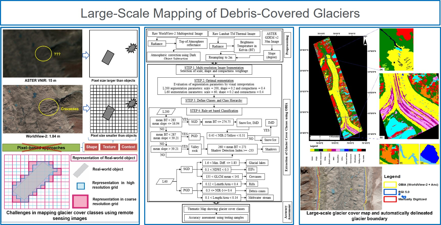
| Mean Brightness Temperature (K) | To differentiate between SGD, PGD, and valley rock | SGD has a lower temperature as compared to PGD and valley rock due to the underlying glacier ice (Figure 5A). |
| To map snow/ice and IMD | In the thermal infrared region, IMD shows a higher spectral response than snow/ice because IMD contains debris that raises its temperature (Figure 4). | |
| To map shadows | The temperature of shadows is remarkably lower than all the other classes (Figure 4). | |
| Mean Slope (Degrees) | To differentiate SGD from PGD and valley rock | The glacier surface (SGD) is formed at lower slopes than the non-glacier surface (PGD and valley rock). |
| NIR-2/Yellow | To differentiate IMD from snow/ice | Snow/ice and IMD have a high spectral response in the yellow wavelength region, whereas it is low in the NIR-2 region. Further, the spectral response of snow/ice in both these regions is relatively higher than that of IMD (Figure 4). Therefore, band ratio NIR-2/Yellow was developed to distinguish IMD from snow/ice. |
| Shadow Detection Index | To map shadows and EIFs | Shadow detection index developed by Shahi et al. [46] using WorldView-2 multispectral data could effectively map shadows. The formula for the Shadow detection index is defined in Equation (1). |
| Max. Diff. | To map glacial lakes | Max. Diff. attribute [47] is the result of the difference between the maximum value of an object and its minimum mean value. The mean values of all layers (WorldView-2 reflectance imagery, brightness temperature, and slope) belonging to an object are compared to get the maximum and minimum values. Subsequently, the result is divided by the brightness. Glacial lakes show the highest values of Max. Diff. attribute. |
| NDWI | To map EIFs | NDWI used in this study is a spectral index developed by Wolf [48] using WorldView-2 multispectral data. The formulation of NDWI is as given in Equation (2). EIFs were successfully mapped using NDWI. |
| GLCM mean | To map crevasses | GLCM mean is the average expressed in terms of the GLCM. The pixel data are weighted by the frequency of its occurrence in combination with a certain neighbor pixel data [49]. Crevasses were mapped using GLCM mean. |
| NIR-1 | To map debris cones | The spectral response of debris cones is higher than that of PGD in the NIR-1 region (Figure 4). Therefore, debris cones are classified using mean values of NIR-1. |
| Length/Area | To map rills and meltwater streams | The length/area is a geometric attribute, which defines elongation [47]. Since rills and meltwater streams (that originate from the snout) are elongated features, length/area attribute was used to classify these classes. |
| Class Name | Traditional Pixel-Based Error Matrix | Area-Weighted Error Matrix | ||
|---|---|---|---|---|
| User’s Accuracy (%) | Producer’s Accuracy (%) | User’s Accuracy (%) | Producer’s Accuracy (%) | |
| Snow/Ice | 92.6 | 92.6 | 99.4 | 98.9 |
| IMD | 88.5 | 92.0 | 91.1 | 98.9 |
| SGD | 92.3 | 96.6 | 99.1 | 96.8 |
| PGD | 66.7 | 80.0 | 94.5 | 85.4 |
| Valley rock | 88.3 | 89.5 | 95.2 | 91.9 |
| Meltwater streams | 100 | 85.7 | 100.0 | 92.1 |
| Glacial lakes | 96.9 | 93.9 | 98.4 | 96.8 |
| EIFs | 100 | 81.1 | 100.0 | 85.4 |
| Crevasses | 100 | 81.1 | 100.0 | 94.3 |
| Debris cones | 81.5 | 84.6 | 89.8 | 90.0 |
| Rills | 100.0 | 81.1 | 100.0 | 88.1 |
| Shadows | 90.0 | 93.1 | 96.0 | 98.1 |
| Class | Rulesets | Sub-Classes and Their Rulesets | |
|---|---|---|---|
| SGD | mean BT < 283 mean slope < 30 | Supraglacial lakes | 1.5 < Max. Diff. < 2.0 |
| Snow/Ice + IMD | mean BT ≤ 273 mean slope < 16 | ||
| If 1.4 < Max. Diff. < 1.7, then IMD else Snow/Ice | |||
| PGD | mean BT ≥ 283 slope < 28 | If 279 < mean BT < 285, then PGD else debris cones | |
| Valley rock | slope > 35 | Shadows | 99 < brightness < 113 |
| Refinement | Class | Rulesets | Grow regions as |
| SGD | relative border to PGD >0.1 | PGD | |
| PGD | relative area of SGD >0.4 | SGD | |
| Class Name | Area-Weighted Error Matrix | |
|---|---|---|
| User’s Accuracy (%) | Producer’s Accuracy (%) | |
| Snow/Ice | 96.2 | 89.3 |
| IMD | 92.3 | 85.7 |
| SGD | 94.4 | 98.8 |
| PGD | 78.1 | 85.2 |
| Valley rock | 95.7 | 80.4 |
| Glacial lakes | 100.0 | 92.9 |
| Debris cones | 91.7 | 88.0 |
| Shadows | 100.0 | 96.0 |
| Class | Rulesets | Sub-Classes and Their Rulesets | ||
| SGD | mean BT < 285 mean slope < 23 | Supraglacial lakes | 1.5 < Max. Diff. < 2.0 | |
| EIFs | 0.13 < NDWI < 0.26 | |||
| Snow/Ice + IMD | 261 < mean BT < 282 | If mean BT < 276 and brightness > 600, then Snow/Ice, else IMD. | ||
| PGD | mean BT < 287 15 < mean slope < 40 | Rills | 0.13 < Length/Area < 0.55 | |
| Meltwater streams | 0.09 < Length/Area < 0.24 | |||
| Debris cones | 500 ≤ NIR-1 ≤ 600 | |||
| Periglacial lakes | 1.5 < Max. Diff. < 1.6 | |||
| Valley rock | mean slope > 40 mean BT > 283 | Shadows | −337 < SDI < −36 | |
| Refinement | Class | Rulesets | Grow regions as | |
| SGD | relative border to PGD >0.3 | PGD | ||
| PGD | relative area of SGD >0.9 | SGD | ||
| Meltwater streams | 0.1 < NDWI < 0.18 | PGD | ||
| Class Name | Area-Weighted Error Matrix | |
|---|---|---|
| User’s Accuracy (%) | Producer’s Accuracy (%) | |
| Snow/Ice | 98.6 | 100.0 |
| IMD | 100.0 | 89.1 |
| SGD | 98.5 | 100.0 |
| PGD | 89.5 | 94.0 |
| Valley rock | 96.3 | 90.4 |
| Meltwater streams | 96.3 | 94.3 |
| Glacial lakes | 87.3 | 100.0 |
| EIFs | 100.0 | 69.0 |
| Debris cones | 88.4 | 98.1 |
| Rills | 100.0 | 81.4 |
| Shadows | 99.8 | 100.0 |
| Glacier Name | Data | Bias (km2) | Percent Error (%) | ||
|---|---|---|---|---|---|
| RGI 6.0 | MD | RGI 6.0 | MD | ||
| Gangotri | WorldView-2 + ancillary dataset | 0.41 | 0.25 | 1.79 | 1.09 |
| LISS-4 + ancillary dataset | 0.68 | 0.63 | 3.51 | 3.26 | |
| Bara Shigri | WorldView-2 + ancillary dataset | 0.54 | 0.03 | 16.62 | 1.09 |
Publisher’s Note: MDPI stays neutral with regard to jurisdictional claims in published maps and institutional affiliations. |
© 2022 by the authors. Licensee MDPI, Basel, Switzerland. This article is an open access article distributed under the terms and conditions of the Creative Commons Attribution (CC BY) license (https://creativecommons.org/licenses/by/4.0/).
Share and Cite
Mitkari, K.V.; Arora, M.K.; Tiwari, R.K.; Sofat, S.; Gusain, H.S.; Tiwari, S.P. Large-Scale Debris Cover Glacier Mapping Using Multisource Object-Based Image Analysis Approach. Remote Sens. 2022, 14, 3202. https://doi.org/10.3390/rs14133202
Mitkari KV, Arora MK, Tiwari RK, Sofat S, Gusain HS, Tiwari SP. Large-Scale Debris Cover Glacier Mapping Using Multisource Object-Based Image Analysis Approach. Remote Sensing. 2022; 14(13):3202. https://doi.org/10.3390/rs14133202
Chicago/Turabian StyleMitkari, Kavita V., Manoj K. Arora, Reet Kamal Tiwari, Sanjeev Sofat, Hemendra S. Gusain, and Surya Prakash Tiwari. 2022. "Large-Scale Debris Cover Glacier Mapping Using Multisource Object-Based Image Analysis Approach" Remote Sensing 14, no. 13: 3202. https://doi.org/10.3390/rs14133202
APA StyleMitkari, K. V., Arora, M. K., Tiwari, R. K., Sofat, S., Gusain, H. S., & Tiwari, S. P. (2022). Large-Scale Debris Cover Glacier Mapping Using Multisource Object-Based Image Analysis Approach. Remote Sensing, 14(13), 3202. https://doi.org/10.3390/rs14133202