
Remote Estimation of Water Clarity and Suspended Particulate Matter in Qinghai Lake from 2001 to 2020 Using MODIS Images

 , , , and
Abstract
:1. Introduction
2. Study Area and Data
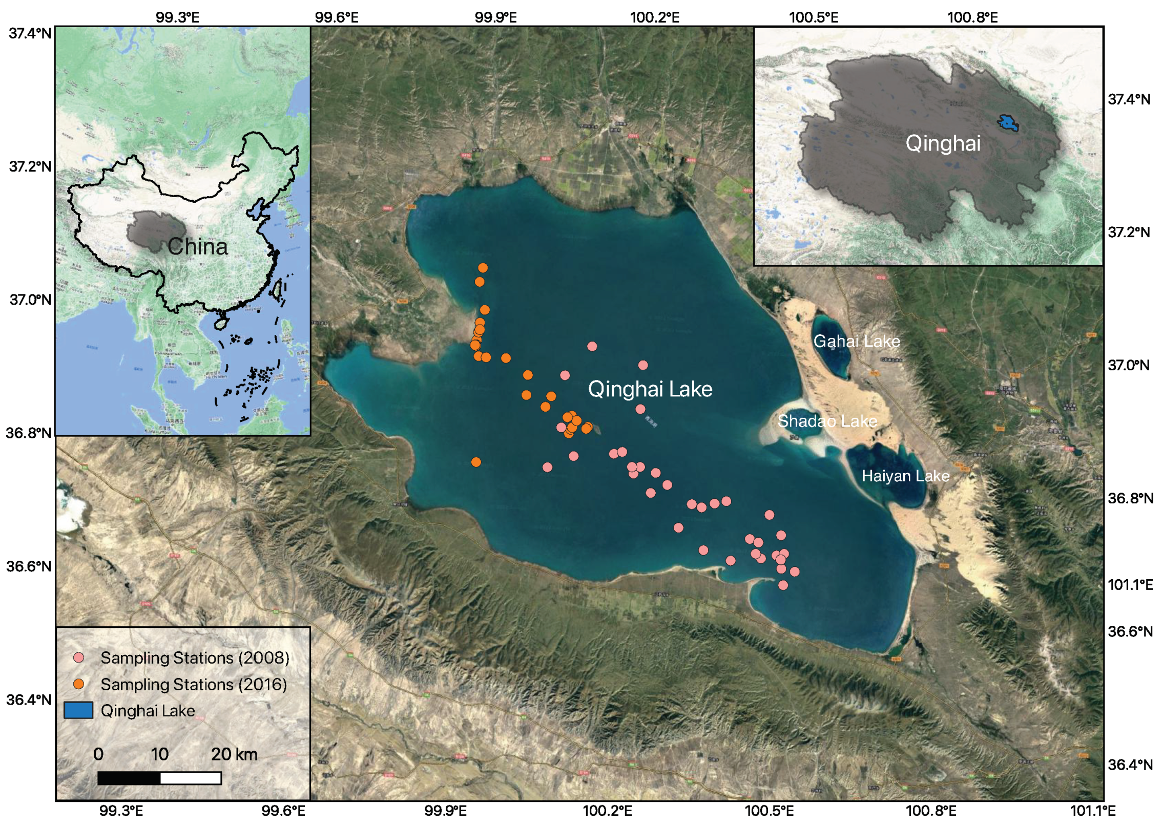
2.1. Study Area
2.2. Field Data
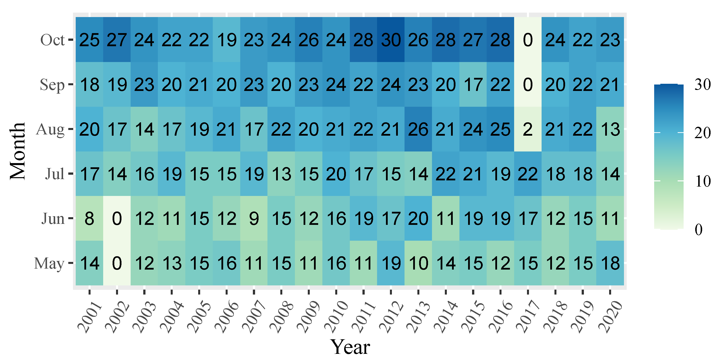
2.3. MODIS Data
3. Methods and Models
3.1. Atmospheric Correction Models
3.2. Estimation of
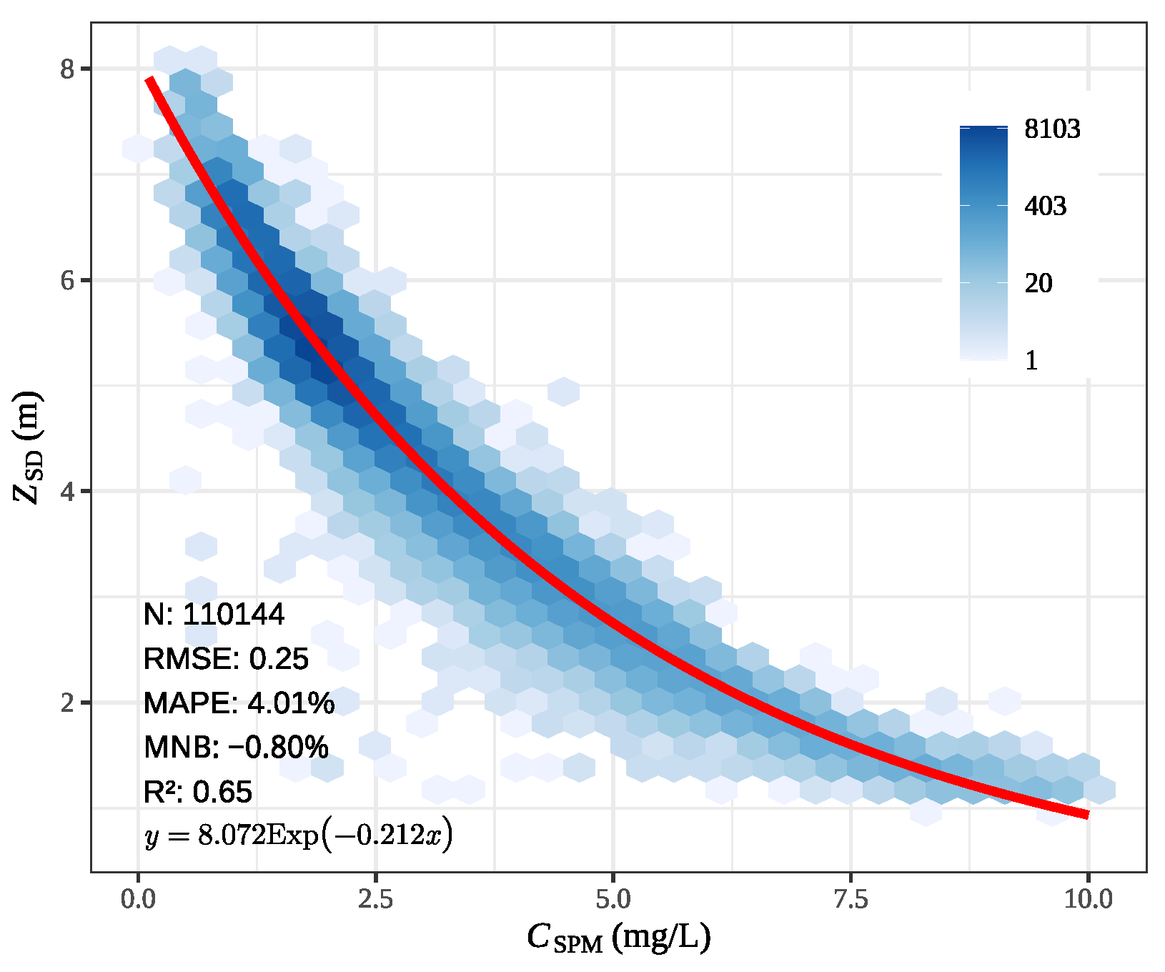
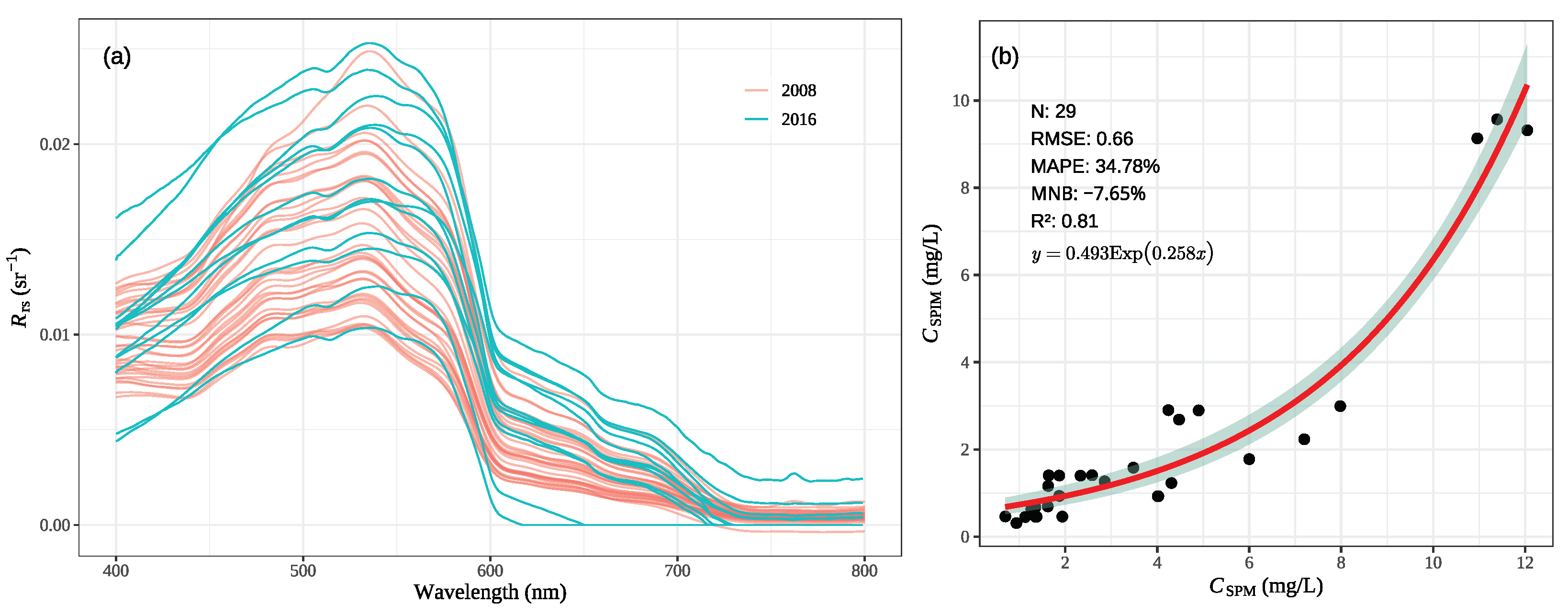
3.3. Estimation of
3.4. Accuracy Assessment
3.5. Statistical Analysis
4. Results
4.1. General Properties of Qinghai Lake
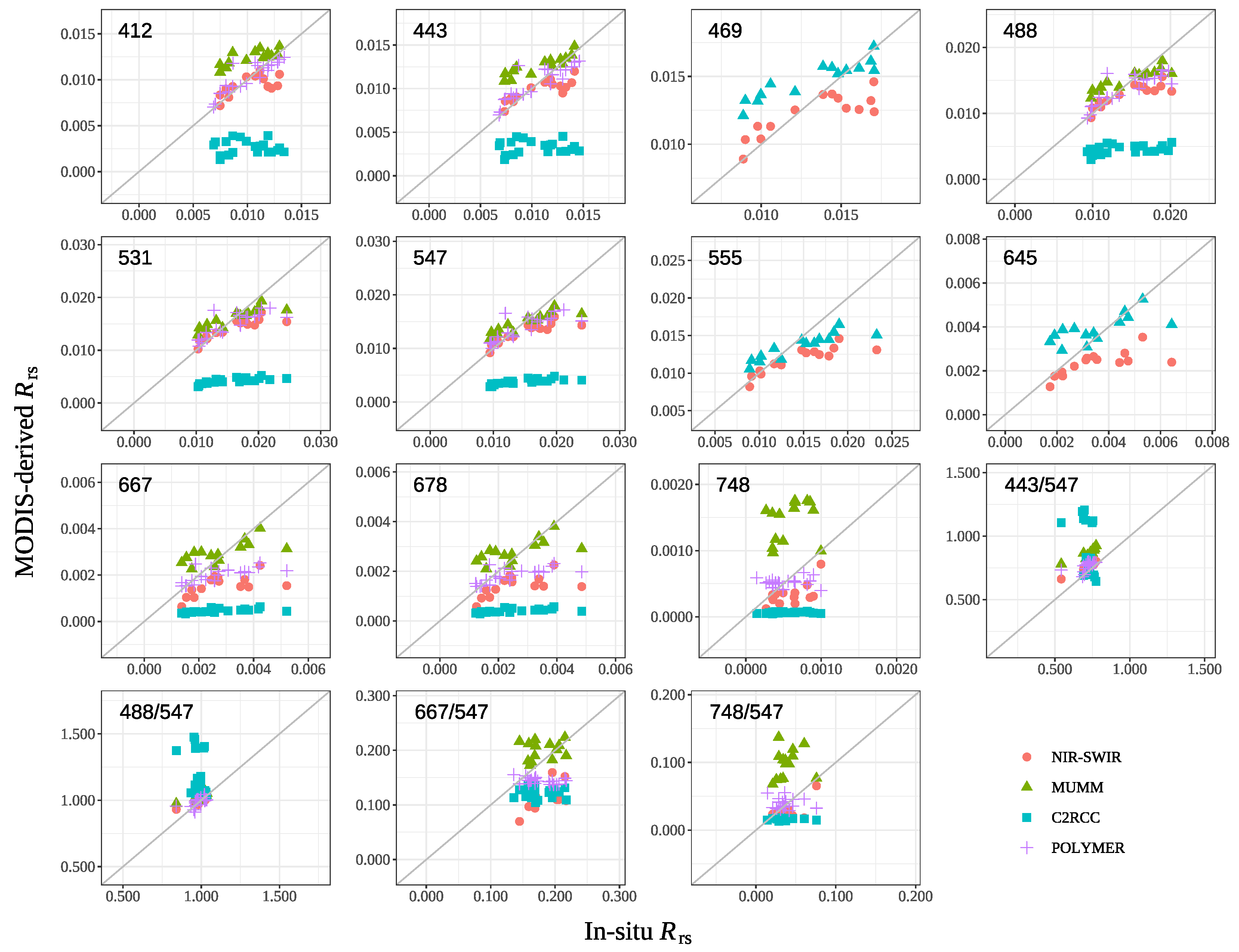
4.2. Accuracy of Atmospheric Correction
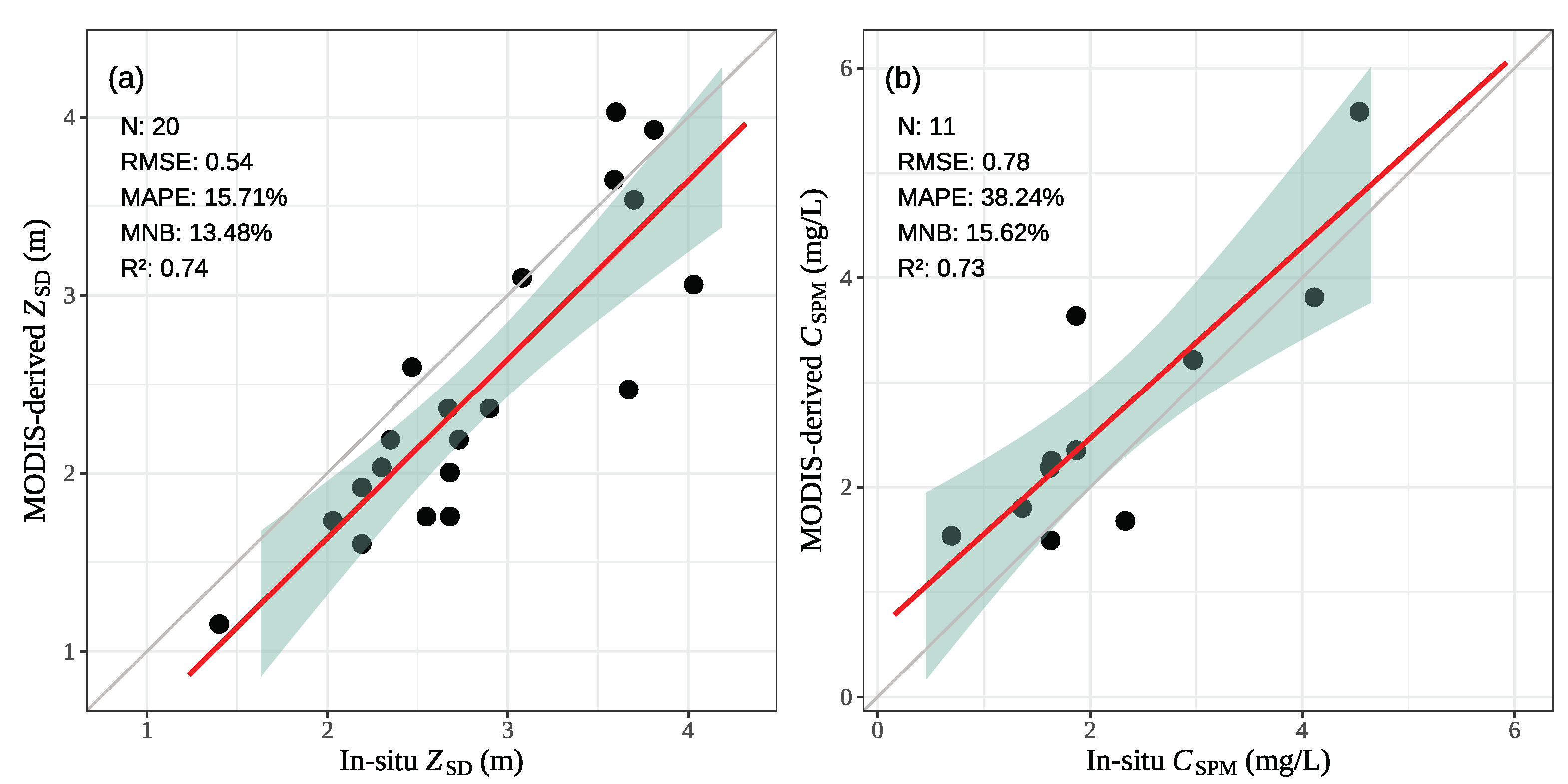
4.3. Estimation of and
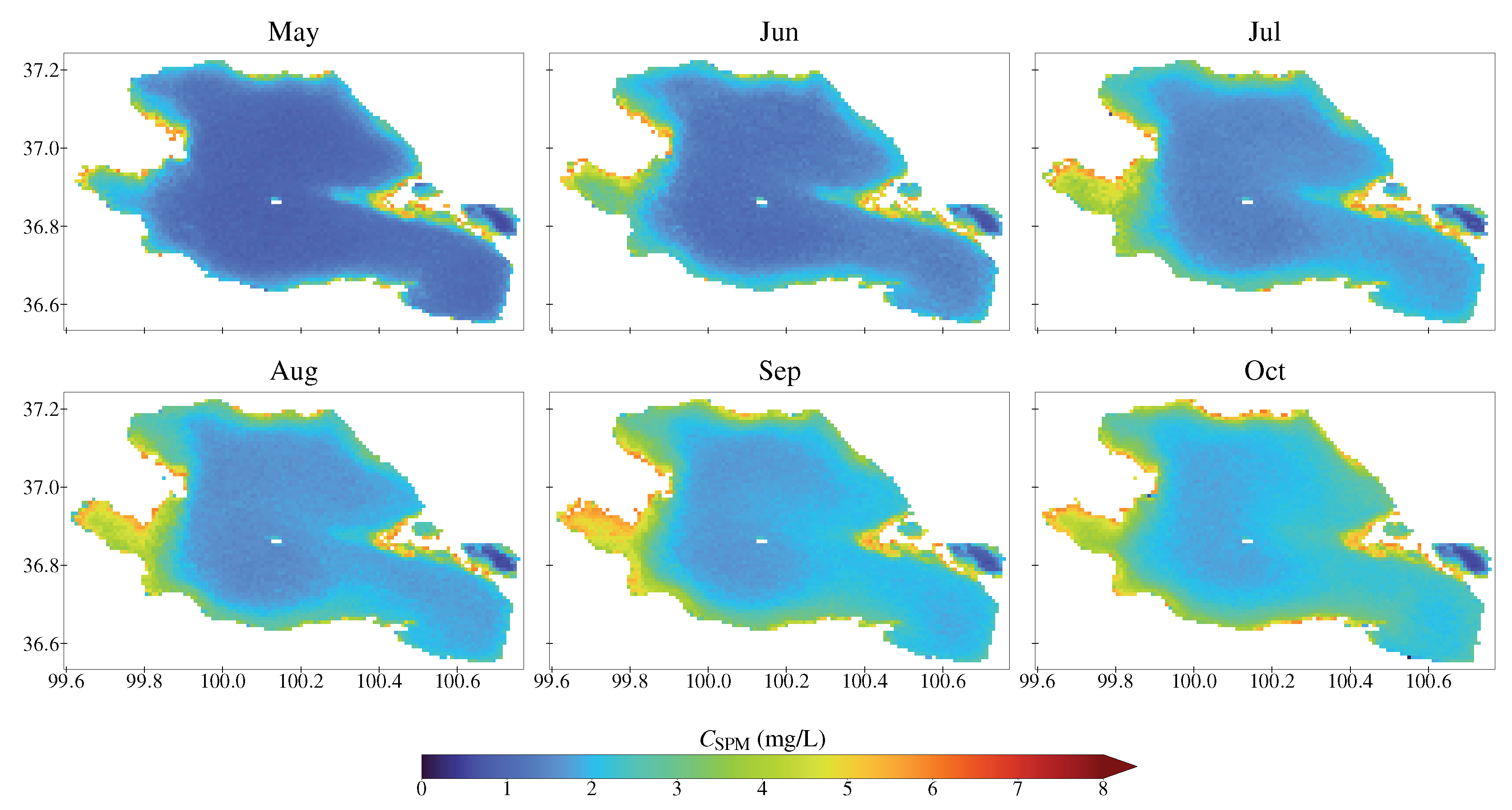
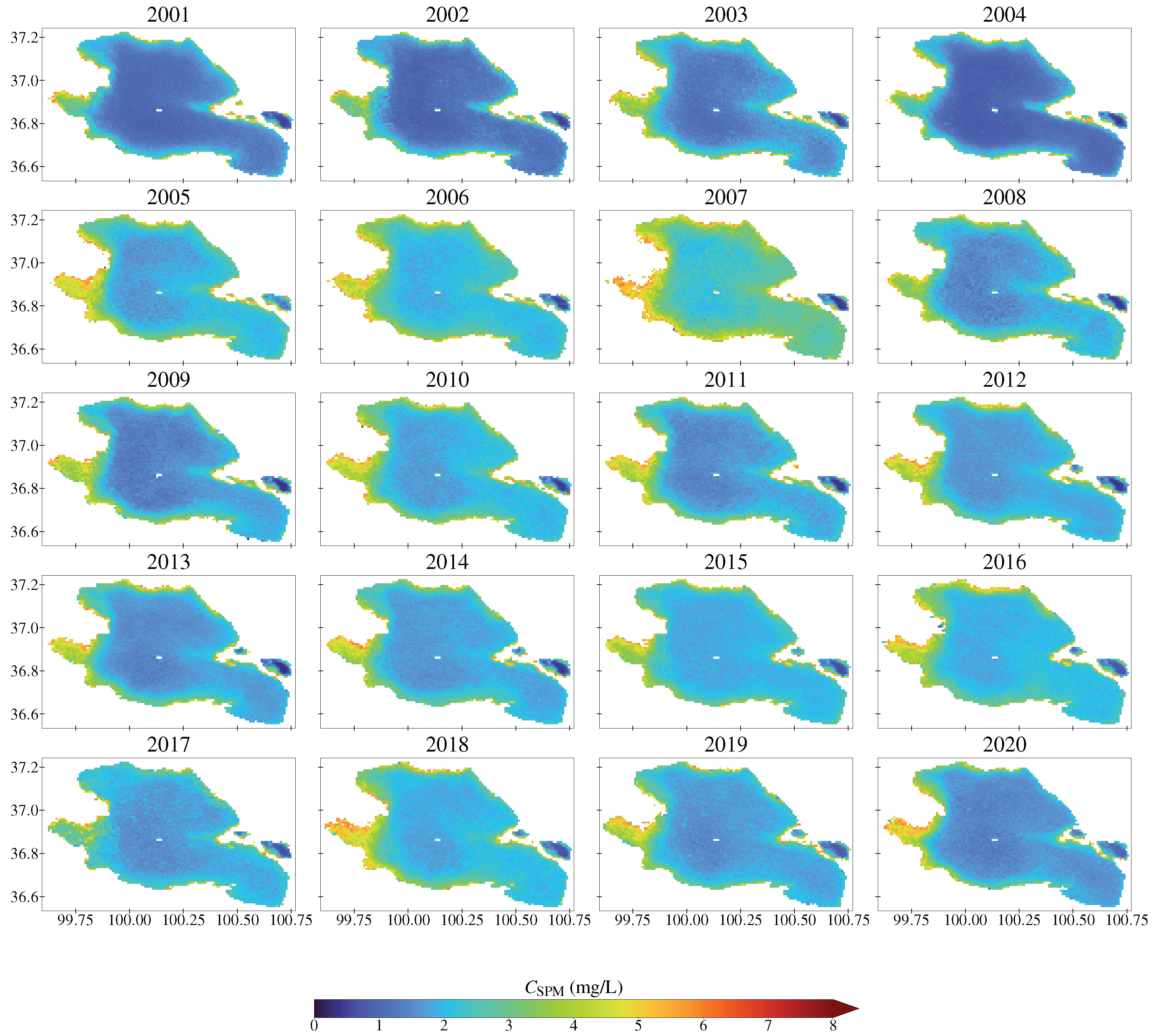
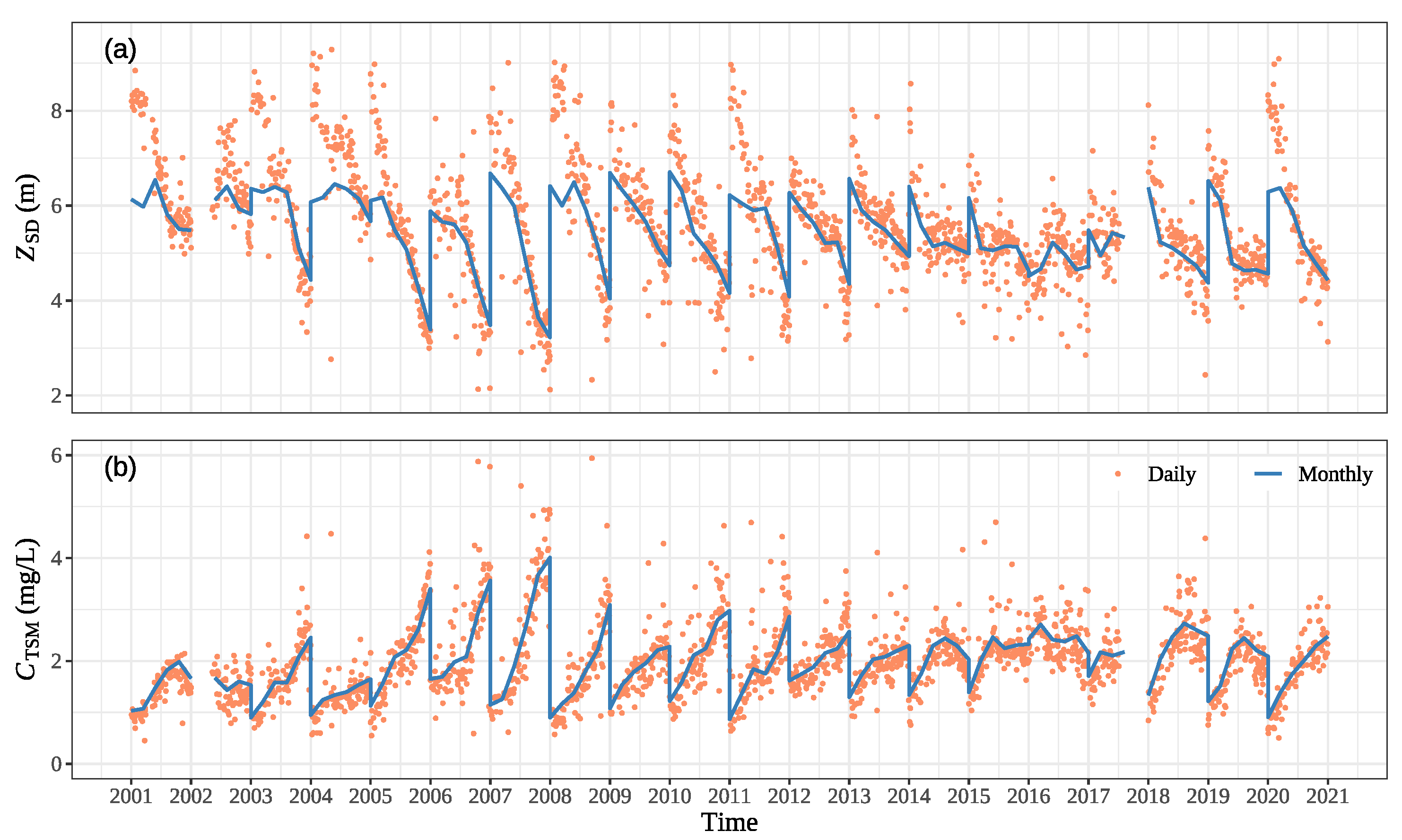
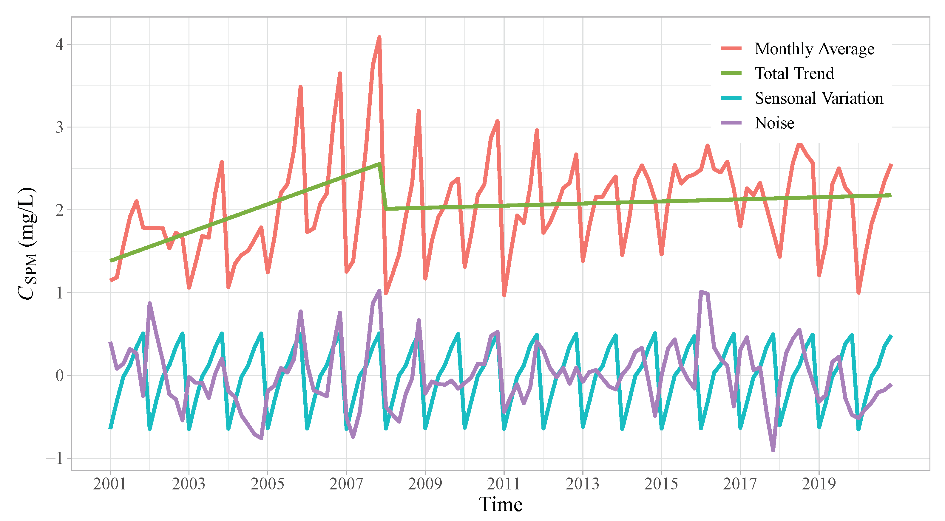
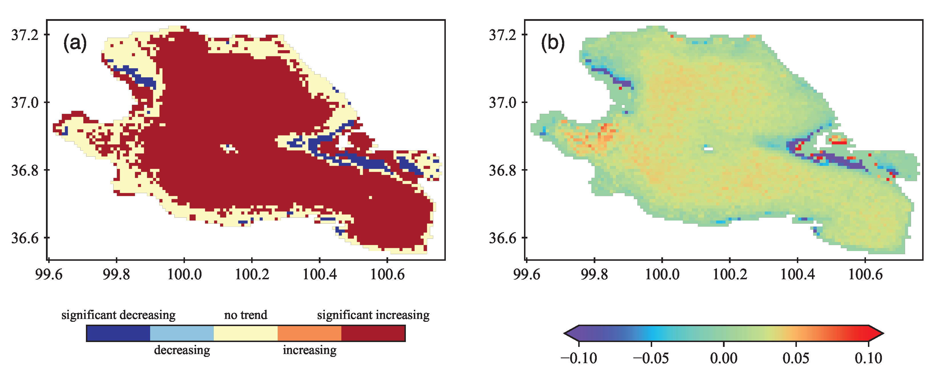
4.4. Spatial and Temporal Variation of
5. Discussion
6. Conclusions
Author Contributions
Funding
Data Availability Statement
Conflicts of Interest
References
- Ma, R.; Duan, H.; Hu, C.; Feng, X.; Li, A.; Ju, W.; Jiang, J.; Yang, G. A half-century of changes in China’s lakes: Global warming or human influence? Geophys. Res. Lett. 2010, 37, L24106. [Google Scholar] [CrossRef]
- Hou, X.; Feng, L.; Duan, H.; Chen, X.; Sun, D.; Shi, K. Fifteen-year monitoring of the turbidity dynamics in large lakes and reservoirs in the middle and lower basin of the Yangtze River, China. Remote Sens. Environ. 2017, 190, 107–121. [Google Scholar] [CrossRef]
- Woolway, R.I.; Kraemer, B.M.; Lenters, J.D.; Merchant, C.J.; O’Reilly, C.M.; Sharma, S. Global lake responses to climate change. Nat. Rev. Earth Environ. 2020, 1, 388–403. [Google Scholar] [CrossRef]
- Bhateria, R.; Jain, D. Water quality assessment of lake water: A review. Sustain. Water Resour. Manag. 2016, 2, 161–173. [Google Scholar] [CrossRef] [Green Version]
- Shen, M.; Duan, H.; Cao, Z.; Xue, K.; Qi, T.; Ma, J.; Liu, D.; Song, K.; Huang, C.; Song, X. Sentinel-3 OLCI observations of water clarity in large lakes in eastern China: Implications for SDG 6.3.2 evaluation. Remote Sens. Environ. 2020, 247, 111950. [Google Scholar] [CrossRef]
- Hou, X.; Feng, L.; Dai, Y.; Hu, C.; Gibson, L.; Tang, J.; Lee, Z.; Wang, Y.; Cai, X.; Liu, J.; et al. Global mapping reveals increase in lacustrine algal blooms over the past decade. Nat. Geosci. 2022, 15, 130–134. [Google Scholar] [CrossRef]
- de Paul Obade, V.; Moore, R. Synthesizing water quality indicators from standardized geospatial information to remedy water security challenges: A review. Environ. Int. 2018, 119, 220–231. [Google Scholar] [CrossRef]
- Ma, T.; Zhao, N.; Ni, Y.; Yi, J.; Wilson John, P.; He, L.; Du, Y.; Pei, T.; Zhou, C.; Song, C.; et al. China’s improving inland surface water quality since 2003. Sci. Adv. 2020, 6, eaau3798. [Google Scholar] [CrossRef] [Green Version]
- Ao, H.; Wu, C.; Xiong, X.; Jing, L.; Huang, X.; Zhang, K.; Liu, J. Water and sediment quality in Qinghai Lake, China: A revisit after half a century. Environ. Monit. Assess. 2014, 186, 2121–2133. [Google Scholar] [CrossRef]
- Ji, S.; Xingqi, L.; Sumin, W.; Matsumoto, R. Palaeoclimatic changes in the Qinghai Lake area during the last 18,000 years. Quat. Int. 2005, 136, 131–140. [Google Scholar] [CrossRef]
- Colman, S.M.; Yu, S.Y.; An, Z.; Shen, J.; Henderson, A.C.G. Late Cenozoic climate changes in China’s western interior: A review of research on Lake Qinghai and comparison with other records. Quat. Sci. Rev. 2007, 26, 2281–2300. [Google Scholar] [CrossRef] [Green Version]
- Tang, L.; Duan, X.; Kong, F.; Zhang, F.; Zheng, Y.; Li, Z.; Mei, Y.; Zhao, Y.; Hu, S. Influences of climate change on area variation of Qinghai Lake on Qinghai-Tibetan Plateau since 1980s. Sci. Rep. 2018, 8, 7331. [Google Scholar] [CrossRef] [PubMed] [Green Version]
- Fan, C.; Song, C.; Li, W.; Liu, K.; Cheng, J.; Fu, C.; Chen, T.; Ke, L.; Wang, J. What drives the rapid water-level recovery of the largest lake (Qinghai Lake) of China over the past half century? J. Hydrol. 2021, 593, 125921. [Google Scholar] [CrossRef]
- Cai, Y.; Ke, C.Q.; Duan, Z. Monitoring ice variations in Qinghai Lake from 1979 to 2016 using passive microwave remote sensing data. Sci. Total. Environ. 2017, 607-608, 120–131. [Google Scholar] [CrossRef]
- Qi, Y.; Lian, X.; Wang, H.; Zhang, J.; Yang, R. Dynamic mechanism between human activities and ecosystem services: A case study of Qinghai lake watershed, China. Ecol. Indic. 2020, 117, 106528. [Google Scholar] [CrossRef]
- Dong, H.; Song, Y.; Zhang, M. Hydrological trend of Qinghai Lake over the last 60 years: Driven by climate variations or human activities? J. Water Clim. Chang. 2018, 10, 524–534. [Google Scholar] [CrossRef]
- Hongmei, D.; Song, Y. Shrinkage history of Lake Qinghai and causes during the last 52 years. In Proceedings of the 2011 International Symposium on Water Resource and Environmental Protection, Xi’an, China, 20–22 May 2011; Volume 1, pp. 446–449. [Google Scholar] [CrossRef]
- Fang, J.; Li, G.; Rubinato, M.; Ma, G.; Zhou, J.; Jia, G.; Yu, X.; Wang, H. Analysis of Long-Term Water Level Variations in Qinghai Lake in China. Water 2019, 11, 2136. [Google Scholar] [CrossRef] [Green Version]
- Xiao, F.; Ling, F.; Du, Y.; Feng, Q.; Yan, Y.; Chen, H. Evaluation of spatial-temporal dynamics in surface water temperature of Qinghai Lake from 2001 to 2010 by using MODIS data. J. Arid Land 2013, 5, 452–464. [Google Scholar] [CrossRef]
- Qi, M.; Yao, X.; Li, X.; Duan, H.; Gao, Y.; Liu, J. Spatiotemporal characteristics of Qinghai Lake ice phenology between 2000 and 2016. J. Geogr. Sci. 2019, 29, 115–130. [Google Scholar] [CrossRef] [Green Version]
- Li, C.; Li, Q.; Zhao, L.; Ge, S.; Chen, D.; Dong, Q.; Zhao, X. Land-use effects on organic and inorganic carbon patterns in the topsoil around Qinghai Lake basin, Qinghai-Tibetan Plateau. CATENA 2016, 147, 345–355. [Google Scholar] [CrossRef]
- Li, J.; Gong, J.; Guldmann, J.M.; Li, S.; Zhu, J. Carbon Dynamics in the Northeastern Qinghai-Tibetan Plateau from 1990 to 2030 Using Landsat Land Use/Cover Change Data. Remote Sens. 2020, 12, 528. [Google Scholar] [CrossRef] [Green Version]
- Cao, S.; Cao, G.; Feng, Q.; Han, G.; Lin, Y.; Yuan, J.; Wu, F.; Cheng, S. Alpine wetland ecosystem carbon sink and its controls at the Qinghai Lake. Environ. Earth Sci. 2017, 76, 210. [Google Scholar] [CrossRef]
- Feng, L.; Liu, J.; Ali, T.A.; Li, J.; Li, J.; Kuang, X. Impacts of the decreased freeze-up period on primary production in Qinghai Lake. Int. J. Appl. Earth Obs. Geoinf. 2019, 83, 101915. [Google Scholar] [CrossRef]
- Arabi, B.; Salama, M.S.; Wernand, M.R.; Verhoef, W. Remote sensing of water constituent concentrations using time series of in situ hyperspectral measurements in the Wadden Sea. Remote Sens. Environ. 2018, 216, 154–170. [Google Scholar] [CrossRef]
- Mouw, C.B.; Greb, S.; Aurin, D.; DiGiacomo, P.M.; Lee, Z.; Twardowski, M.; Binding, C.; Hu, C.; Ma, R.; Moore, T.; et al. Aquatic color radiometry remote sensing of coastal and inland waters: Challenges and recommendations for future satellite missions. Remote Sens. Environ. 2015, 160, 15–30. [Google Scholar] [CrossRef]
- Wang, X.; Yang, W. Water quality monitoring and evaluation using remote sensing techniques in China: A systematic review. Ecosyst. Health Sustain. 2019, 5, 47–56. [Google Scholar] [CrossRef] [Green Version]
- Odermatt, D.; Gitelson, A.; Brando, V.E.; Schaepman, M. Review of constituent retrieval in optically deep and complex waters from satellite imagery. Remote Sens. Environ. 2012, 118, 116–126. [Google Scholar] [CrossRef] [Green Version]
- Rodríguez-López, L.; Duran-Llacer, I.; González-Rodríguez, L.; Cardenas, R.; Urrutia, R. Retrieving Water Turbidity in Araucanian Lakes (South-Central Chile) Based on Multispectral Landsat Imagery. Remote Sens. 2021, 13, 3133. [Google Scholar] [CrossRef]
- Liu, C.; Zhu, L.; Li, J.; Wang, J.; Ju, J.; Qiao, B.; Ma, Q.; Wang, S. The increasing water clarity of Tibetan lakes over last 20 years according to MODIS data. Remote Sens. Environ. 2021, 253, 112199. [Google Scholar] [CrossRef]
- Shi, W.; Wang, M.; Li, J. Water property in high-altitude Qinghai Lake in China. Sci. Remote Sens. 2020, 2, 100012. [Google Scholar] [CrossRef]
- William, L.B.; Vincent, V.S. MODIS: A global imaging spectroradiometer for the Earth Observing System. In Optical Technologies for Aerospace Sensing: A Critical Review; SPIE: Bellingham, DC, USA, 1992; Volume 10269, pp. 280–302. [Google Scholar] [CrossRef]
- Moses, W.J.; Sterckx, S.; Montes, M.J.; De Keukelaere, L.; Knaeps, E. Atmospheric Correction for Inland Waters. In Bio-Optical Modeling and Remote Sensing of Inland Waters; Mishra, D.R., Ogashawara, I., Gitelson, A.A., Eds.; Elsevier: Amsterdam, The Netherlands, 2017; pp. 69–100. [Google Scholar] [CrossRef]
- Vidot, J.; Santer, R. Atmospheric correction for inland waters—Application to SeaWiFS. Int. J. Remote Sens. 2005, 26, 3663–3682. [Google Scholar] [CrossRef]
- Li, H.; He, X.; Shanmugam, P.; Bai, Y.; Wang, D.; Huang, H.; Zhu, Q.; Gong, F. Semi-analytical algorithms of ocean color remote sensing under high solar zenith angles. Opt. Express 2019, 27, A800–A817. [Google Scholar] [CrossRef] [PubMed]
- Stock, A. Satellite mapping of Baltic Sea Secchi depth with multiple regression models. Int. J. Appl. Earth Obs. Geoinf. 2015, 40, 55–64. [Google Scholar] [CrossRef]
- Cao, Z.; Duan, H.; Shen, M.; Ma, R.; Xue, K.; Liu, D.; Xiao, Q. Using VIIRS/NPP and MODIS/Aqua data to provide a continuous record of suspended particulate matter in a highly turbid inland lake. Int. J. Appl. Earth Obs. Geoinf. 2018, 64, 256–265. [Google Scholar] [CrossRef]
- Han, Z.; Gu, X.; Zuo, X.; Bi, K.; Shi, S. Semi-Empirical Models for the Bidirectional Water-Leaving Radiance: An Analysis of a Turbid Inland Lake. Front. Environ. Sci. 2022, 9, 557. [Google Scholar] [CrossRef]
- Lee, Z.; Shang, S.; Hu, C.; Du, K.; Weidemann, A.; Hou, W.; Lin, J.; Lin, G. Secchi disk depth: A new theory and mechanistic model for underwater visibility. Remote Sens. Environ. 2015, 169, 139–149. [Google Scholar] [CrossRef] [Green Version]
- Lee, Z.; Carder, K.L.; Arnone, R.A. Deriving inherent optical properties from water color: A multiband quasi-analytical algorithm for optically deep waters. Appl. Opt. 2002, 41, 5755–5772. [Google Scholar] [CrossRef]
- Lee, Z.P.; Du, K.P.; Arnone, R. A model for the diffuse attenuation coefficient of downwelling irradiance. J. Geophys. Res. Oceans 2005, 110, C02016. [Google Scholar] [CrossRef]
- Bi, R.; Zhang, H.; Li, H.; Chang, F.; Duan, L.; He, Y.; Zhang, H.; Wen, X.; Zhou, Y. Characteristics and changes of water quality parameters of Qinghai Lake in 2015. J. Water Resour. Res. 2018, 7, 74–83. [Google Scholar] [CrossRef]
- Mueller, J.L.; Morel, A.; Frouin, R.; Davis, C.; Arnone, R.; Carder, K.; Lee, Z.P.; Steward, R.G.; Hooker, S.; Mobley, C.D.; et al. Ocean Optics Protocols For Satellite Ocean Color Sensor Validation, Revision 4. Volume III: Radiometric Measurements and Data Analysis Protocols; Goddard Space Flight Center: Greenbelt, MD, USA, 2003. [Google Scholar] [CrossRef]
- Wang, M. Remote sensing of the ocean contributions from ultraviolet to near-infrared using the shortwave infrared bands: Simulations. Appl. Opt. 2007, 46, 1535–1547. [Google Scholar] [CrossRef]
- Wang, M.; Shi, W. The NIR–SWIR combined atmospheric correction approach for MODIS ocean color data processing. Opt. Express 2007, 15, 15722–15733. [Google Scholar] [CrossRef] [Green Version]
- Ruddick, K.G.; Ovidio, F.; Rijkeboer, M. Atmospheric correction of SeaWiFS imagery for turbid coastal and inland waters. Appl. Opt. 2000, 39, 897–912. [Google Scholar] [CrossRef] [PubMed] [Green Version]
- Steinmetz, F.; Deschamps, P.Y.; Ramon, D. Atmospheric correction in presence of sun glint: Application to MERIS. Opt. Express 2011, 19, 9783–9800. [Google Scholar] [CrossRef] [Green Version]
- Brockmann, C.; Doerffer, R.; Peters, M.; Kerstin, S.; Embacher, S.; Ruescas, A. Evolution of the C2RCC Neural Network for Sentinel 2 and 3 for the Retrieval of Ocean Colour Products in Normal and Extreme Optically Complex Waters. In Proceedings of the Living Planet Symposium, Prague, Czech Republic, 9–13 May 2016; Volume 740, p. 54. [Google Scholar]
- Siegel, D.A.; Wang, M.; Maritorena, S.; Robinson, W. Atmospheric correction of satellite ocean color imagery: The black pixel assumption. Appl. Opt. 2000, 39, 3582–3591. [Google Scholar] [CrossRef] [PubMed]
- Wang, M.; Son, S.; Shi, W. Evaluation of MODIS SWIR and NIR–SWIR atmospheric correction algorithms using SeaBASS data. Remote Sens. Environ. 2009, 113, 635–644. [Google Scholar] [CrossRef]
- Wang, D.; Ma, R.; Xue, K.; Loiselle, S.A. The Assessment of Landsat-8 OLI Atmospheric Correction Algorithms for Inland Waters. Remote Sens. 2019, 11, 169. [Google Scholar] [CrossRef] [Green Version]
- Zhang, M.; Hu, C.; Barnes, B.B. Performance of POLYMER Atmospheric Correction of Ocean Color Imagery in the Presence of Absorbing Aerosols. IEEE Trans. Geosci. Remote Sens. 2019, 57, 6666–6674. [Google Scholar] [CrossRef]
- Yu, X.; Lee, Z.; Shen, F.; Wang, M.; Wei, J.; Jiang, L.; Shang, Z. An empirical algorithm to seamlessly retrieve the concentration of suspended particulate matter from water color across ocean to turbid river mouths. Remote Sens. Environ. 2019, 235, 111491. [Google Scholar] [CrossRef]
- Warren, M.A.; Simis, S.G.H.; Martinez-Vicente, V.; Poser, K.; Bresciani, M.; Alikas, K.; Spyrakos, E.; Giardino, C.; Ansper, A. Assessment of atmospheric correction algorithms for the Sentinel-2A MultiSpectral Imager over coastal and inland waters. Remote Sens. Environ. 2019, 225, 267–289. [Google Scholar] [CrossRef]
- Wu, G.; De Leeuw, J.; Skidmore, A.K.; Prins, H.H.T.; Liu, Y. Comparison of MODIS and Landsat TM5 images for mapping tempo-spatial dynamics of Secchi disk depths in Poyang Lake National Nature Reserve, China. Int. J. Remote Sens. 2008, 29, 2183–2198. [Google Scholar] [CrossRef]
- Kratzer, S.; Brockmann, C.; Moore, G. Using MERIS full resolution data to monitor coastal waters—A case study from Himmerfjärden, a fjord-like bay in the northwestern Baltic Sea. Remote Sens. Environ. 2008, 112, 2284–2300. [Google Scholar] [CrossRef]
- Binding, C.E.; Greenberg, T.A.; Watson, S.B.; Rastin, S.; Gould, J. Long term water clarity changes in North America’s Great Lakes from multi-sensor satellite observations. Limnol. Oceanogr. 2015, 60, 1976–1995. [Google Scholar] [CrossRef]
- Doron, M.; Babin, M.; Hembise, O.; Mangin, A.; Garnesson, P. Ocean transparency from space: Validation of algorithms estimating Secchi depth using MERIS, MODIS and SeaWiFS data. Remote Sens. Environ. 2011, 115, 2986–3001. [Google Scholar] [CrossRef]
- Preisendorfer, R.W. Secchi disk science: Visual optics of natural waters. Limnol. Oceanogr. 1986, 31, 909–926. [Google Scholar] [CrossRef] [Green Version]
- Lee, Z.; Shang, S.; Qi, L.; Yan, J.; Lin, G. A semi-analytical scheme to estimate Secchi-disk depth from Landsat-8 measurements. Remote Sens. Environ. 2016, 177, 101–106. [Google Scholar] [CrossRef]
- Lee, Z.; Shang, S.; Du, K.; Wei, J. Resolving the long-standing puzzles about the observed Secchi depth relationships. Limnol. Oceanogr. 2018, 63, 2321–2336. [Google Scholar] [CrossRef]
- Blackwell, H.R. Contrast Thresholds of the Human Eye. J. Opt. Soc. Am. 1946, 36, 624–643. [Google Scholar] [CrossRef]
- Lee, Z.; Hu, C.; Shang, S.; Du, K.; Lewis, M.; Arnone, R.; Brewin, R. Penetration of UV-visible solar radiation in the global oceans: Insights from ocean color remote sensing. J. Geophys. Res. Ocean. 2013, 118, 4241–4255. [Google Scholar] [CrossRef] [Green Version]
- IOCCG. Update of the Quasi-Analytical Algorithm (QAA_v6). Technical Report, IOCCG Group. 2014. Available online: https://www.ioccg.org/groups/Software_OCA/QAA_v6_2014209.pdf (accessed on 20 April 2021).
- Shang, S.; Lee, Z.; Shi, L.; Lin, G.; Wei, G.; Li, X. Changes in water clarity of the Bohai Sea: Observations from MODIS. Remote Sens. Environ. 2016, 186, 22–31. [Google Scholar] [CrossRef] [Green Version]
- Feng, L.; Hou, X.; Zheng, Y. Monitoring and understanding the water transparency changes of fifty large lakes on the Yangtze Plain based on long-term MODIS observations. Remote Sens. Environ. 2019, 221, 675–686. [Google Scholar] [CrossRef]
- Mao, Z.; Chen, J.; Pan, D.; Tao, B.; Zhu, Q. A regional remote sensing algorithm for total suspended matter in the East China Sea. Remote Sens. Environ. 2012, 124, 819–831. [Google Scholar] [CrossRef]
- Dogliotti, A.I.; Ruddick, K.G.; Nechad, B.; Doxaran, D.; Knaeps, E. A single algorithm to retrieve turbidity from remotely-sensed data in all coastal and estuarine waters. Remote Sens. Environ. 2015, 156, 157–168. [Google Scholar] [CrossRef] [Green Version]
- Han, B.; Loisel, H.; Vantrepotte, V.; Mériaux, X.; Bryére, P.; Ouillon, S.; Dessailly, D.; Xing, Q.; Zhu, J. Development of a Semi-Analytical Algorithm for the Retrieval of Suspended Particulate Matter from Remote Sensing over Clear to Very Turbid Waters. Remote Sens. 2016, 8, 211. [Google Scholar] [CrossRef] [Green Version]
- Novoa, S.; Doxaran, D.; Ody, A.; Vanhellemont, Q.; Lafon, V.; Lubac, B.; Gernez, P. Atmospheric Corrections and Multi-Conditional Algorithm for Multi-Sensor Remote Sensing of Suspended Particulate Matter in Low-to-High Turbidity Levels Coastal Waters. Remote Sens. 2017, 9, 61. [Google Scholar] [CrossRef] [Green Version]
- Jiang, D.; Matsushita, B.; Pahlevan, N.; Gurlin, D.; Lehmann, M.K.; Fichot, C.G.; Schalles, J.; Loisel, H.; Binding, C.; Zhang, Y.; et al. Remotely estimating total suspended solids concentration in clear to extremely turbid waters using a novel semi-analytical method. Remote Sens. Environ. 2021, 258, 112386. [Google Scholar] [CrossRef]
- Hendrik, B.; Hakvoort, J.H.M.; Donze, M. Optical properties of pure water. In Ocean Optics XII; SPIE: Bellingham, DC, USA, 1994; Volume 2258. [Google Scholar] [CrossRef]
- Balasubramanian, S.V.; Pahlevan, N.; Smith, B.; Binding, C.; Schalles, J.; Loisel, H.; Gurlin, D.; Greb, S.; Alikas, K.; Randla, M.; et al. Robust algorithm for estimating total suspended solids (TSS) in inland and nearshore coastal waters. Remote Sens. Environ. 2020, 246, 111768. [Google Scholar] [CrossRef]
- Verbesselt, J.; Hyndman, R.; Zeileis, A.; Culvenor, D. Phenological change detection while accounting for abrupt and gradual trends in satellite image time series. Remote Sens. Environ. 2010, 114, 2970–2980. [Google Scholar] [CrossRef] [Green Version]
- Verbesselt, J.; Hyndman, R.; Newnham, G.; Culvenor, D. Detecting trend and seasonal changes in satellite image time series. Remote Sens. Environ. 2010, 114, 106–115. [Google Scholar] [CrossRef]
- Sang, Y.F.; Wang, Z.; Liu, C. Comparison of the MK test and EMD method for trend identification in hydrological time series. J. Hydrol. 2014, 510, 293–298. [Google Scholar] [CrossRef]
- Hamed, K.H.; Ramachandra Rao, A. A modified Mann-Kendall trend test for autocorrelated data. J. Hydrol. 1998, 204, 182–196. [Google Scholar] [CrossRef]
- Hipel, K.W.; McLeod, A.I. Time Series Modelling of Water Resources and Environmental Systems; Elsevier: Amsterdam, The Netherlands, 1994. [Google Scholar]
- Hirsch, R.M.; Slack, J.R. A Nonparametric Trend Test for Seasonal Data With Serial Dependence. Water Resour. Res. 1984, 20, 727–732. [Google Scholar] [CrossRef] [Green Version]
- Feng, L.; Hu, C. Land adjacency effects on MODIS Aqua top-of-atmosphere radiance in the shortwave infrared: Statistical assessment and correction. J. Geophys. Res. Ocean. 2017, 122, 4802–4818. [Google Scholar] [CrossRef]
- Jia, J.; Chen, Q.; Ren, H.; Lu, R.; He, H.; Gu, P. Phytoplankton Composition and Their Related Factors in Five Different Lakes in China: Implications for Lake Management. Int. J. Environ. Res. Public Health 2022, 19, 3135. [Google Scholar] [CrossRef]
- Wang, H.; Long, H.; Li, X.; Yu, F. Evaluation of changes in ecological security in China’s Qinghai Lake Basin from 2000 to 2013 and the relationship to land use and climate change. Environ. Earth Sci. 2014, 72, 341–354. [Google Scholar] [CrossRef]
- Xinhua. China’s Largest Saltwater Lake Sees Water Area Expand. 2021. Available online: http://www.chinadaily.com.cn/a/202110/21/WS617115eea310cdd39bc705fe.html (accessed on 22 April 2022).


| Models | Metrics | 412 | 443 | 469 | 488 | 531 | 547 | 555 | 645 | 667 | 678 | 748 |
|---|---|---|---|---|---|---|---|---|---|---|---|---|
| NIR–SWIR | RMSE | 0.0018 | 0.0019 | 0.0022 | 0.0030 | 0.0034 | 0.0036 | 0.0040 | 0.0016 | 0.0016 | 0.0014 | 0.0003 |
| MAPE | 12.43% | 12.28% | 11.73% | 13.06% | 12.95% | 14.27% | 16.75% | 28.84% | 41.66% | 41.73% | 40.51% | |
| MNB | −10.34% | −9.28% | 7.65% | −14.14% | 12.75% | −16.02% | −21.99% | −48.98% | −84.98% | −85.65% | −91.05% | |
| 0.39 | 0.71 | 0.69 | 0.74 | 0.76 | 0.76 | 0.75 | 0.50 | 0.35 | 0.34 | 0.40 | ||
| MUMM | RMSE | 0.0025 | 0.0024 | 0.0024 | 0.0022 | 0.0027 | 0.0028 | 0.0030 | 0.0011 | 0.0009 | 0.0008 | 0.0009 |
| MAPE | 23.39% | 21.38% | 17.85% | 14.38% | 14.31% | 15.18% | 15.87% | 29.71% | 28.98% | 29.69% | 183.21% | |
| MNB | 17.02% | 15.18% | 11.20% | 3.38% | 1.12% | −1.17% | −6.00% | 10.34% | 6.39% | 8.37% | 58.42% | |
| 0.58 | 0.78 | 0.84 | 0.83 | 0.79 | 0.79 | 0.79 | 0.49 | 0.47 | 0.45 | 0.07 | ||
| C2RCC | RMSE | 0.0077 | 0.0076 | 0.0103 | 0.0120 | 0.0116 | 0.0024 | 0.0023 | 0.0005 | |||
| MAPE | 72.42% | 66.59% | 66.54% | 71.92% | 72.96% | 80.80% | 81.34% | 86.26% | ||||
| MNB | −308.62% | −231.76% | −215.74% | −267.90% | −283.27% | −470.72% | −489.84% | −776.75% | ||||
| 0.00 | 0.00 | 0.16 | 0.57 | 0.59 | 0.34 | 0.32 | 0.08 | |||||
| POLYMER | RMSE | 0.0010 | 0.0014 | 0.0022 | 0.0028 | 0.0029 | 0.0011 | 0.0010 | 0.0002 | |||
| MAPE | 8.24% | 10.86% | 10.77% | 12.18% | 13.23% | 24.56% | 24.23% | 47.70% | ||||
| MNB | 2.25% | 1.86% | -4.25% | -4.35% | −5.73% | −32.41% | −31.59% | −4.55% | ||||
| 0.78 | 0.75 | 0.70 | 0.66 | 0.64 | 0.48 | 0.47 | 0.01 |
| Models | RMSE | MAPE | MNB | |
|---|---|---|---|---|
| Wu (2008) | 0.73 | 26.27% | −36.96% | 0.08 |
| Kratzer (2008) | 2.28 | 88.54% | −958.05% | 0.03 |
| Binding (2015) | 18.10 | 717.87% | 87.62% | 0.01 |
| Lee (2015) | 0.54 | 15.71% | −18.30% | 0.74 |
| Models | RMSE | MAPE | MNB | |
|---|---|---|---|---|
| Mao (2012) | 6.46 | 360.70% | 64.38% | 0.09 |
| Dogliotti (2015) | 2.66 | 46.13% | −21.28% | 0.12 |
| Han (2016) | 5.07 | 234.55% | 56.75% | 0.13 |
| Novoa (2017) | 2.89 | 118.21% | 28.74% | 0.13 |
| Yu (2019) | 3.65 | 64.44% | −298.64% | 0.19 |
| Jiang (2021) | 0.78 | 38.24% | 15.62% | 0.73 |
Publisher’s Note: MDPI stays neutral with regard to jurisdictional claims in published maps and institutional affiliations. |
© 2022 by the authors. Licensee MDPI, Basel, Switzerland. This article is an open access article distributed under the terms and conditions of the Creative Commons Attribution (CC BY) license (https://creativecommons.org/licenses/by/4.0/).
Share and Cite
Tan, Z.; Cao, Z.; Shen, M.; Chen, J.; Song, Q.; Duan, H. Remote Estimation of Water Clarity and Suspended Particulate Matter in Qinghai Lake from 2001 to 2020 Using MODIS Images. Remote Sens. 2022, 14, 3094. https://doi.org/10.3390/rs14133094
Tan Z, Cao Z, Shen M, Chen J, Song Q, Duan H. Remote Estimation of Water Clarity and Suspended Particulate Matter in Qinghai Lake from 2001 to 2020 Using MODIS Images. Remote Sensing. 2022; 14(13):3094. https://doi.org/10.3390/rs14133094
Chicago/Turabian StyleTan, Zhenyu, Zhigang Cao, Ming Shen, Jun Chen, Qingjun Song, and Hongtao Duan. 2022. "Remote Estimation of Water Clarity and Suspended Particulate Matter in Qinghai Lake from 2001 to 2020 Using MODIS Images" Remote Sensing 14, no. 13: 3094. https://doi.org/10.3390/rs14133094
APA StyleTan, Z., Cao, Z., Shen, M., Chen, J., Song, Q., & Duan, H. (2022). Remote Estimation of Water Clarity and Suspended Particulate Matter in Qinghai Lake from 2001 to 2020 Using MODIS Images. Remote Sensing, 14(13), 3094. https://doi.org/10.3390/rs14133094