Latent Low-Rank Projection Learning with Graph Regularization for Feature Extraction of Hyperspectral Images

Abstract

Due to the great benefit of rich spectral information, hyperspectral images (HSIs) have been successfully applied in many fields. However, some problems of concern also limit their further applications, such as high dimension and expensive labeling. To address these issues, an unsupervised latent low-rank projection learning with graph regularization (LatLRPL) method is presented for feature extraction and classification of HSIs in this paper, in which discriminative features can be extracted from the view of latent space by decomposing the latent low-rank matrix into two different matrices, also benefiting from the preservation of intrinsic subspace structures by the graph regularization. Different from the graph embedding-based methods that need two phases to obtain the low-dimensional projections, one step is enough for LatLRPL by constructing the integrated projection learning model, reducing the complexity and simultaneously improving the robustness. To improve the performance, a simple but effective strategy is exploited by conducting the local weighted average on the pixels in a sliding window for HSIs. Experiments on the Indian Pines and Pavia University datasets demonstrate the superiority of the proposed LatLRPL method.

1. Introduction

Depending on hundreds of spectral bands captured by the hyperspectral imaging systems [1], hyperspectral images (HSIs) can better present the substance compositions of regions of interest from the view of pixel-level representations. Accordingly, lots of fields have made attempts to apply HSIs, such as agricultural monitoring, urban planning, and military reconnaissance, showing promising results. One problem that has to be faced directly when enjoying the advantages of HSIs is the high spectral dimensionality [2,3,4], which usually brings much more computational cost and degrades the performance to some extent. Feature extraction [5,6,7,8] can effectively solve this problem by reducing the dimensionality of HSIs and simultaneously preserving the significant information. Due to the great success in feature extraction and classification of natural images [9,10], the deep learning-based methods have attracted lots of attention [11,12,13]. Some researchers also attempted to utilize deep learning methods to process hyperspectral images, showing superiority in many tasks [14,15]. In this paper, the traditional machine learning-based methods are of concern.

Among all the feature extraction methods, principal component analysis (PCA) [16] is the most popular and also an effective unsupervised method to reduce the dimensionality of the data by maximizing the variance in low-dimensional space. Due to the lack of prior knowledge of samples, PCA may not perform very well. To overcome this problem, some supervised feature extraction methods have been proposed. For example, linear discriminant analysis (LDA) [17] was developed by maximizing the trace ratio of between-class and within-class scatter matrices, which is improved by local Fisher’s discriminant analysis (LFDA) [18].

To make full use of the intrinsic structure expressed implicitly in the data, some manifold learning-based methods [19,20] have been proposed. Locality preserving projection (LPP) [21] was designed to preserve the similar local relationships among samples from the original high-dimensional space to the low-dimensional space, which evolved from locally linear embedding (LLE) [22]. Neighborhood preserving embedding (NPE) [23] can capture the intrinsic subspace structures by minimizing the reconstructed error between one sample and its neighbors, which is extended from Laplacian eigenmaps (LE) [24].

A unified framework called graph embedding was proposed in [25] by constructing two graphs, which takes the aforementioned methods into account. In this framework, the graph weight matrix plays the most important role in the quality of the low-dimensional features. Traditional methods, such as k-nearest neighbor and $\epsilon$-radius ball, are usually influenced by noise. Due to the good robustness and promising performance, sparse representation (SR) [26] has attracted increasing attention for image classification [27] and target detection [28] since it was proposed for the first time. Therefore, some researchers employ the SR coefficient to construct the weight matrix, generating many classical feature extraction methods for HSIs. For example, sparse graph embedding (SGE) [29] was proposed to construct the sparse graph for feature extraction by solving a $l_1$ optimization problem. In [30], sparsity preserving projection (SPP) was proposed by constructing the adjacency weight from a modified SR method. Subsequently, sparse graph-based discriminant analysis (SGDA) [31] was developed by exploiting the prior label information, which is further extended to block SGDA by constructing a within-class graph. Based on SGDA, He et al. [32] pointed out that the locality constraint could improve the discriminative ability of a sparse coefficient and constructed the weighted SGDA model. Due to the great computational burden brought about by the optimization of the $l_1$ norm, Ly et al. [33] replaced the $l_1$ norm with the $l_2$ regularization by borrowing the idea from [34], improving the computational efficiency.

SR-based graph embedding methods capture the intrinsic structure of the data from the perspective of locality, which, however, ignores the positive effect from the view of the global information. In [35], Liu et al. proposed a low-rank representation (LRR) model to explore the global structure information of the data and extended it to a low-rank graph embedding model for unsupervised feature extraction. Commonly, the data structure can be presented by exploiting both local and global information [36,37]. Accordingly, one method presented in [38] takes both sparse regularization and low-rank regularization into consideration to construct the low-rank and sparse graph for the extraction of discriminative low-dimensional features. Following SLGDA, some distinguished works are proposed. For instance, to deal with the nonlinear property of the hyperspectral data, one feature extraction method named classical kernel SLGDA [39] was proposed for HSIs to advance the computational efficiency by accelerating the process of kernel transformation with a virtual kernel technique. In [40], to fully exploit the spatial information of the hyperspectral data, the tensor theory was introduced into the work [38], resulting in an effective spatial-spectral feature extraction method that can learn the local and global structures of the hyperspectral data.

Graph embedding-based feature extraction methods can effectively extract low-dimensional features from the hyperspectral data; however, there are still some challenges that require conquering. First, the key point of these methods is the construction of adjacent graphs that represent the intrinsic subspace structure. The aforementioned methods addressed this problem using KNN, SR, and LRR, which cannot present satisfying results. Second, graph embedding-based methods acquire low-dimensional features through two disconnected steps, i.e., graph construction and projection optimization, which loses some valuable and discriminative information.

In the process of hyperspectral imaging, various kinds of noise will have a negative influence on the quality of HSIs [41,42,43]. In other words, some pixels can be grossly corrupted. In this case, both SR and LRR are not competent at preserving the intrinsic subspace structure of the hyperspectral data. To address this issue, Liu et al. [44] proposed a latent low-rank representation (LatLRR) model by considering the data structure from two views, i.e., column space and row space. When the data are corrupted in the column space, it can also be recovered from the row space. Depending on this advantage of LatLRR, Pan et al. [45] proposed two data recovery models from the spectral domain and spatial domain for the hyperspectral data. Another big difference between LRR and LatLRR is that LatLRR is able to extract salient features of the data without graph construction. This inborn advantage shows great significance in face recognition, which can characterize some salient and discriminative features of one’s face, such as eyes and noses. However, the dimension of the extracted salient features is the same as that of the original data [46]. Strictly speaking, it is actually not a common feature extraction method. In addition, LatLRR still limits its view on the preservation of the global structure of the data.

To overcome these problems, a novel latent low-rank projection learning with graph regularization (LatLRPL) method is proposed for unsupervised feature extraction of HSIs in this paper. In LatLRPL, two different representation matrices with the same dimension are adopted to decompose the salient projection matrix in LatLRR, forming a discriminative projection matrix with a controllable feature dimension. To capture the local intrinsic structure of hyperspectral data, both original space and low-dimensional space are considered. On the one hand, a spectral constraint matrix from the original space is constructed to enhance the discriminative ability of corresponding subspaces. On the other hand, manifold learning on the learned low-dimensional space is exploited as the graph regularization to preserve the local subspace structures. Experiments on two common hyperspectral datasets show the superiority of the proposed LatLRPL method. The main contributions of this paper can be summarized as follows.

(1) Compared with LatLRR, LatLRPL is able to learn discriminative features with the desired dimensionality for the hyperspectral data, accomplishing the dimensionality reduction in the real sense. In addition, local structure and global structure can be well preserved in the learned low-dimensional feature space.

(2) Different from graph embedding-based methods that require two steps to obtain the projection, LatLRPL integrates representation learning and projection learning into one framework, thereby improving the robustness and computational efficiency.

(3) To better preserve the local intrinsic subspace structures, regularization on both the original space and the learned low-dimensional space is integrated into LatLRPL by using spectral constraint and graph regularization, respectively.

The remainder of this paper is organized as follows. Section 2 introduces some related work. The framework and optimization of the proposed LatLRPL method are elaborated in Section 3. In Section 4, experimental results and analysis are provided. Section 5 provides the conclusions for this paper.

2. Related Work

In this section, some classical work about feature extraction, such as low-rank representation, latent low-rank representation, and locality preserving projection, has been briefly reviewed in regard to their motivations and mathematic theories, which is referential for the design of the proposed method. To formulate the related work clearly, definitions about some variables are first provided. Given an HSI $\mathbf{H}\in {\mathbb{R}}^{H\times W\times D}$ with D spectral bands, $\mathbf{X}=[{\mathbf{x}}_1,{\mathbf{x}}_2,\dots ,{\mathbf{x}}_N]\in {\mathbb{R}}^{D\times N}$ is defined as a sample set containing N samples, in which ${\mathbf{x}}_i\in {\mathbb{R}}^{D\times 1}$ denotes the ith sample.

2.1. Low-Rank Representation for Feature Extraction

Sparse representation (SR) attempts to represent one sample by using a few labeled samples in the dictionary. Although it has achieved promising performance in many fields, SR can not present the global data structure. As such, Liu et al. [35] first proposed the low-rank representation (LRR) by representing one sample set jointly, which can be formulated as

$$\begin{array}{c}\hfill \underset{\mathbf{Z},\mathbf{E}}{min}{\parallel \mathbf{Z}\parallel }_{*}+\lambda {\parallel \mathbf{E}\parallel }_{2,1}s.t.\mathbf{X}=\mathbf{X}\mathbf{Z}+\mathbf{E}\end{array}$$

(1)

where ${\parallel ·\parallel }_{*}$ denotes the nuclear norm used to approximate the rank of one matrix, ${\parallel \mathbf{E}\parallel }_{2,1}$ is the $l_{2,1}$ norm used to represent sample-specific corruptions, defined as ${\parallel \mathbf{E}\parallel }_{2,1}={\sum }_{j=1}^N\sqrt{{\sum }_{i=1}^d{\left({\mathbf{E}}_{ij}\right)}^2}$, $\mathbf{Z}$ denotes the lowest rank reconstructed coefficient matrix with the global structure information captured, $\lambda$ is the regularization parameter. Similar to sparse graph embedding [29], the low-rank coefficient matrix can be used to construct the low-rank graph for feature extraction by employing the graph embedding framework.

2.2. Latent Low-Rank Representation for Feature Extraction

In practical applications, the observed data are usually contaminated by various kinds of noise. More seriously, some samples are corrupted badly. LRR shows good performance in the preservation of global data structure; however, it only considers this from the column space. When the data are deadly corrupted, LRR does not perform effectively. To overcome this shortcoming, Liu et al. [44] proposed a latent low-rank representation (LatLRR) model by taking both the column space and the row space of the data into account. Experimental results indicate that LatLRR is very effective when coping with corrupted data. The objective function of LatLRR is defined as

$$\begin{array}{cc}\hfill & \underset{\mathbf{Z},\mathbf{L},\mathbf{E}}{min}{\parallel \mathbf{Z}\parallel }_{*}+{\parallel \mathbf{L}\parallel }_{*}+\lambda {\parallel \mathbf{E}\parallel }_{2,1},\hfill \\ \hfill & s.t.\mathbf{X}=\mathbf{X}\mathbf{Z}+\mathbf{L}\mathbf{X}+\mathbf{E},\hfill \end{array}$$

(2)

where $\mathbf{Z}\in {\mathbb{R}}^{N\times N}$ is the column coefficient matrix that reconstructs the data from the column space, and $\mathbf{L}\in {\mathbb{R}}^{D\times D}$ is the row coefficient matrix that reconstructs the data from the row space. This is the reason why LatLRR performs better than LRR for the corrupted data. Additionally, $\mathbf{L}$ can also be exploited as the projection matrix to extract the salient feature from the data, which has been deeply researched in face recognition. However, from the objective function $\left(2\right)$, it can be seen that the salient feature $\mathbf{L}\mathbf{X}$ has the same dimension as the original data $\mathbf{X}$. This is not preferred in the case of low-dimensional feature extraction.

2.3. Locality Preserving Projection for Feature Extraction

Locality preserving projection (LPP), as one popular manifold learning method, shows its effectiveness in capturing the local geometric data structure for feature extraction. The nature of LPP is to preserve the local relationship in the original space to the low-dimensional space. For this purpose, a neighbor graph is first constructed by searching the nearest neighbors of one sample. Specifically, the weight factors can be defined as follows.

$$\begin{array}{c}\hfill {\mathbf{W}}_{ij}=\left\{\begin{array}{cc}1,\hfill & if{\mathbf{x}}_i\in N_k\left({\mathbf{x}}_j\right)or{\mathbf{x}}_j\in N_k\left({\mathbf{x}}_i\right)\hfill \\ 0,\hfill & otherwise\hfill \end{array}\right.\end{array}$$

(3)

where $N_k\left({\mathbf{x}}_j\right)$ is a set of k nearest neighbors of ${\mathbf{x}}_i$. When ${\mathbf{x}}_j$ belongs to one of the nearest neighbors of ${\mathbf{x}}_i$, or ${\mathbf{x}}_i$ is in the nearest neighbor set of ${\mathbf{x}}_j$, the weight value between ${\mathbf{x}}_i$ and ${\mathbf{x}}_j$ is defined as 1. Otherwise, 0 is given. The graph weight matrix represents the local relationships of samples in the original space. Then, based on the idea of LPP, its objective function is designed as

$$\begin{array}{cc}\hfill & \underset{{\mathbf{P}}^T\mathbf{X}\mathbf{D}{\mathbf{X}}^T\mathbf{P}}{min}\sum _{i,j=1}^N{\parallel {\mathbf{P}}^T{\mathbf{x}}_i-{\mathbf{P}}^T{\mathbf{x}}_j\parallel }_2^2{\mathbf{W}}_{ij}\hfill \\ \hfill =& \underset{Tr({\mathbf{P}}^T\mathbf{X}\mathbf{D}{\mathbf{X}}^T\mathbf{P}=1)}{min}Tr\left({\mathbf{P}}^T\mathbf{X}\mathbf{L}{\mathbf{X}}^T\mathbf{P}\right)\hfill \end{array}$$

(4)

where $\mathbf{D}$ denotes a diagonal matrix with its ith element defined as ${\mathbf{D}}_{ii}={\sum }_{j=1}^N{\mathbf{W}}_{ij}$, $\mathbf{L}$ denotes the Laplacian matrix with $\mathbf{L}=\mathbf{D}-\mathbf{W}$, and $\mathbf{P}$ is the projection matrix that can preserve the local structure information.

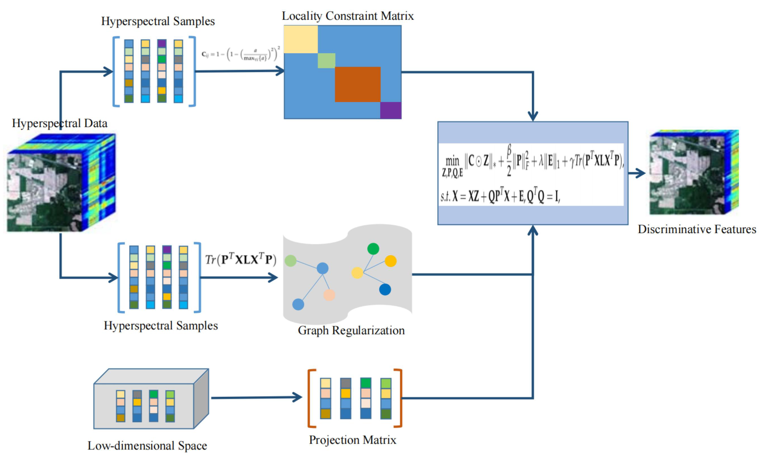
3. Proposed Unsupervised Projection Learning Method

In order to better capture the local and global structure of the hyperspectral data simultaneously, as well as reduce the redundancy of graph embedding-based methods, a novel latent low-rank projection learning with graph regularization (LatLRPL) method is proposed for the feature extraction of HSIs in this section. The model construction and optimization of LatLRPL are formulated explicitly in the following sections.

3.1. Model Construction of LatLRPL

Advantages of LatLRR in processing corrupted data and extracting salient features make it very popular in face recognition, which, however, fails to reduce the dimensionality of the extracted salient feature. To solve this problem, two different matrixes are adopted to decompose the low-rank projection matrix, i.e., $\mathbf{L}=\mathbf{Q}{\mathbf{P}}^T$, with $\mathbf{Q}\in {\mathbb{R}}^{D\times d}$ and $\mathbf{P}\in {\mathbb{R}}^{D\times d}$, and d denotes the number of preserved features. In this paper, $\mathbf{P}$ is exploited as the projection matrix to obtain the low-dimensional salient feature. As such, the model of LatLRR can be transformed as follows.

$$\begin{array}{cc}\hfill & \underset{\mathbf{Z},\mathbf{P},\mathbf{Q},\mathbf{E}}{min}{\parallel \mathbf{Z}\parallel }_{*}+\parallel \mathbf{Q}{\mathbf{P}}^T{\parallel }_{*}+\lambda {\parallel \mathbf{E}\parallel }_{2,1},\hfill \\ \hfill & s.t.\mathbf{X}=\mathbf{X}\mathbf{Z}+\mathbf{Q}{\mathbf{P}}^T\mathbf{X}+\mathbf{E}.\hfill \end{array}$$

(5)

From Equation $\left(5\right)$, we can observe that it is awfully difficult to obtain the solutions of $\mathbf{Q}$ and $\mathbf{P}$. Therefore, the low-rank constraint on $\mathbf{Q}{\mathbf{P}}^T$ by the nuclear norm is relaxed through the Frobenius norm multiplied by a regularization parameter. Correspondingly, Equation $\left(5\right)$ can be changed as

$$\begin{array}{cc}\hfill & \underset{\mathbf{Z},\mathbf{P},\mathbf{Q},\mathbf{E}}{min}{\parallel \mathbf{Z}\parallel }_{*}+\frac{\beta }{2}\parallel \mathbf{Q}{\mathbf{P}}^T{\parallel }_F^2+\lambda {\parallel \mathbf{E}\parallel }_{2,1},\hfill \\ \hfill & s.t.\mathbf{X}=\mathbf{X}\mathbf{Z}+\mathbf{Q}{\mathbf{P}}^T\mathbf{X}+\mathbf{E},{\mathbf{Q}}^T\mathbf{Q}=\mathbf{I},\hfill \end{array}$$

(6)

where $\beta$ is the regularization parameter with a value much less than 1, which can constrain $\parallel \mathbf{Q}{\mathbf{P}}^T{\parallel }_F^2$ to be much more approximate to $\parallel \mathbf{Q}{\mathbf{P}}^T{\parallel }_{*}$ and simultaneously balance the effect of $\parallel \mathbf{Q}{\mathbf{P}}^T{\parallel }_F^2$ in the objective function. To avoid the trivial solution, an orthogonal constraint is imposed on $\mathbf{Q}$.

For simplification, $\parallel \mathbf{Q}{\mathbf{P}}^T{\parallel }_F^2$ can be further manipulated as the following.

$$\begin{array}{cc}\hfill \parallel \mathbf{Q}{\mathbf{P}}^T{\parallel }_F^2& =Tr\left({\left(\mathbf{Q}{\mathbf{P}}^T\right)}^T\left(\mathbf{Q}{\mathbf{P}}^T\right)\right)\hfill \\ \hfill & =Tr\left(\mathbf{P}{\mathbf{Q}}^T\mathbf{Q}{\mathbf{P}}^T\right)\hfill \\ \hfill & =Tr\left(\mathbf{P}{\mathbf{P}}^T\right)\hfill \\ \hfill & =Tr\left({\mathbf{P}}^T\mathbf{P}\right)\hfill \\ \hfill & ={\parallel \mathbf{P}\parallel }_F^2\hfill \end{array}$$

(7)

Based on Equation $\left(7\right)$, problem $\left(6\right)$ is reformulated as

$$\begin{array}{cc}\hfill & \underset{\mathbf{Z},\mathbf{P},\mathbf{Q},\mathbf{E}}{min}{\parallel \mathbf{Z}\parallel }_{*}+\frac{\beta }{2}{\parallel \mathbf{P}\parallel }_F^2+\lambda {\parallel \mathbf{E}\parallel }_1,\hfill \\ \hfill & s.t.\mathbf{X}=\mathbf{X}\mathbf{Z}+\mathbf{Q}{\mathbf{P}}^T\mathbf{X}+\mathbf{E},{\mathbf{Q}}^T\mathbf{Q}=\mathbf{I},\hfill \end{array}$$

(8)

where ${\parallel \mathbf{E}\parallel }_1$ is used to represent sparse random noise by considering the characteristics of the hyperspectral data.

As mentioned above, the low-rank constraint is helpful for capturing the global intrinsic structure, while it fails to reveal the local structure of the data. According to our previous work [47], the locality constraint is applied to advance the representation of the local structure by exploiting the spectral similarity in the hyperspectral data. Based on this, problem $\left(8\right)$ can be rewritten as

$$\begin{array}{cc}\hfill & \underset{\mathbf{Z},\mathbf{P},\mathbf{Q},\mathbf{E}}{min}{\parallel \mathbf{C}\odot \mathbf{Z}\parallel }_{*}+\frac{\beta }{2}{\parallel \mathbf{P}\parallel }_F^2+\lambda {\parallel \mathbf{E}\parallel }_1,\hfill \\ \hfill & s.t.\mathbf{X}=\mathbf{X}\mathbf{Z}+\mathbf{Q}{\mathbf{P}}^T\mathbf{X}+\mathbf{E},{\mathbf{Q}}^T\mathbf{Q}=\mathbf{I},\hfill \end{array}$$

(9)

where $\mathbf{C}$ is the locality constrained matrix, whose elements can be calculated as

$$\begin{array}{c}\hfill {\mathbf{C}}_{ij}=1-{\left(1-{\left(\frac{a}{{max}_{\forall i}\left\{a\right\}}\right)}^2\right)}^2,\end{array}$$

(10)

where $a=dist({\mathbf{x}}_i,{\mathbf{x}}_j)$ denotes the spectral similarity of samples ${\mathbf{x}}_i$ and ${\mathbf{x}}_j$. The local constraint $\mathbf{C}$ can make similar samples represented by similar codes, thus improving the quality of the representation of the local structure.

Different from the spectral constraint, manifold learning is qualified to explore the intrinsic structure of the low-dimensional space. In this paper, the locality preserving projection is utilized as the graph regularization to learn the local structure of the hyperspectral data. As such, the objective function of the proposed LatLRPL method can be finally constructed as follows.

$$\begin{array}{cc}\hfill & \underset{\mathbf{Z},\mathbf{P},\mathbf{Q},\mathbf{E}}{min}{\parallel \mathbf{C}\odot \mathbf{Z}\parallel }_{*}+\frac{\beta }{2}{\parallel \mathbf{P}\parallel }_F^2+\lambda {\parallel \mathbf{E}\parallel }_1+\gamma Tr\left({\mathbf{P}}^T\mathbf{X}\mathbf{L}{\mathbf{X}}^T\mathbf{P}\right),\hfill \\ \hfill & s.t.\mathbf{X}=\mathbf{X}\mathbf{Z}+\mathbf{Q}{\mathbf{P}}^T\mathbf{X}+\mathbf{E},{\mathbf{Q}}^T\mathbf{Q}=\mathbf{I},\hfill \end{array}$$

(11)

where $\gamma$ is one parameter that can control the effect of the graph regularization.

From Equation $\left(11\right)$, on the one hand, projection learning is integrated into a representation learning model, which can effectively improve the efficiency and robustness of projection computation with the desired dimensionality. On the other hand, regularization of the original data space and the low-dimensional feature space is able to capture the local intrinsic structure of the hyperspectral data. Theoretically, discriminative features can indeed be extracted by LatLRPL from the noisy and high-dimensional hyperspectral data. The framework of the proposed LatLRPL method is presented in Figure 1.

3.2. Optimization of LatLRPL

In order to obtain the projection matrix, the alternating direction method of multipliers (ADMM) [48] is used to effectively optimize the objective function of the LatLRPL method. To effectively solve problem $\left(11\right)$, we introduce two variables $\mathbf{A}$ and $\mathbf{B}$ to make the problem separable, generating the following function.

$$\begin{array}{cc}\hfill & \underset{\mathbf{Z},\mathbf{A},\mathbf{P},\mathbf{B},\mathbf{Q},\mathbf{E}}{min}{\parallel \mathbf{C}\odot \mathbf{A}\parallel }_{*}+\frac{\beta }{2}{\parallel \mathbf{P}\parallel }_F^2+\lambda {\parallel \mathbf{E}\parallel }_1+\gamma Tr\left({\mathbf{B}}^T\mathbf{X}\mathbf{L}{\mathbf{X}}^T\mathbf{B}\right),\hfill \\ \hfill & s.t.\mathbf{X}=\mathbf{X}\mathbf{Z}+\mathbf{Q}{\mathbf{P}}^T\mathbf{X}+\mathbf{E},\mathbf{Z}=\mathbf{A},\mathbf{P}=\mathbf{B},{\mathbf{Q}}^T\mathbf{Q}=\mathbf{I}.\hfill \end{array}$$

(12)

For problem $\left(12\right)$, theaugmented Lagrangian function is formulated as

$$\begin{array}{c}\hfill \begin{array}{c}\begin{array}{cc}\hfill & L(\mathbf{Z},\mathbf{A},\mathbf{P},\mathbf{B},\mathbf{Q},\mathbf{E})\hfill \\ \hfill =& {\parallel \mathbf{C}\odot \mathbf{A}\parallel }_{*}+\frac{\beta }{2}{\parallel \mathbf{P}\parallel }_F^2+\lambda {\parallel \mathbf{E}\parallel }_1+\gamma Tr\left({\mathbf{B}}^T\mathbf{X}\mathbf{L}{\mathbf{X}}^T\mathbf{B}\right)+\langle {\mathbf{Y}}_1,\mathbf{X}-\mathbf{X}\mathbf{Z}-\mathbf{Q}{\mathbf{P}}^T\mathbf{X}-\mathbf{E}\rangle \hfill \\ \hfill +& \langle {\mathbf{Y}}_2,\mathbf{Z}-\mathbf{A}\rangle +\langle {\mathbf{Y}}_3,\mathbf{P}-\mathbf{B}\rangle +\frac{\mu }{2}(\parallel \mathbf{X}-\mathbf{X}\mathbf{Z}-\mathbf{Q}{\mathbf{P}}^T{\mathbf{X}-\mathbf{E}\parallel }_F^2{+\parallel \mathbf{Z}-\mathbf{A}\parallel }_F^2{+\parallel \mathbf{P}-\mathbf{B}\parallel }_F^2),\hfill \end{array}\hfill \end{array}\end{array}$$

(13)

where ${\mathbf{Y}}_1$, ${\mathbf{Y}}_2$, and ${\mathbf{Y}}_3$ are Lagrangian multipliers, $\mu$ is a penalty factor.

After some operations, Equation $\left(13\right)$ can be further written as

$$\begin{array}{c}\hfill \begin{array}{c}\begin{array}{cc}\hfill & L(\mathbf{Z},\mathbf{A},\mathbf{P},\mathbf{B},\mathbf{Q},\mathbf{E})\hfill \\ \hfill =& {\parallel \mathbf{C}\odot \mathbf{A}\parallel }_{*}+\frac{\beta }{2}{\parallel \mathbf{P}\parallel }_F^2+{\lambda \parallel \mathbf{E}\parallel }_1+\gamma Tr\left({\mathbf{B}}^T\mathbf{X}\mathbf{L}{\mathbf{X}}^T\mathbf{B}\right)+\frac{\mu }{2}(\parallel \mathbf{X}-\mathbf{X}\mathbf{Z}-\mathbf{Q}{\mathbf{P}}^T\mathbf{X}-\mathbf{E}+\frac{{\mathbf{Y}}_1}{\mu }{\parallel }_F^2\hfill \\ \hfill +& \parallel \mathbf{Z}-\mathbf{A}+\frac{{\mathbf{Y}}_2}{\mu }{\parallel }_F^2+\parallel \mathbf{P}-\mathbf{B}+\frac{{\mathbf{Y}}_3}{\mu }{\parallel }_F^2)\hfill \end{array}\hfill \end{array}\end{array}$$

(14)

ADMM is an iterative optimization method in which variables are updated one by one. Therefore, the $(t+1)$th iterative schemes are shown in the following.

$$\begin{array}{c}\hfill {\mathbf{A}}_{t+1}=\underset{\mathbf{A}}{min}{\parallel \mathbf{C}\odot \mathbf{A}\parallel }_{*}+\frac{{\mu }_t}{2}{\parallel {\mathbf{Z}}_t-\mathbf{A}+\frac{{\mathbf{Y}}_{2,t}}{{\mu }_t}\parallel }_F^2\end{array}$$

(15)

$$\begin{array}{cc}\hfill {\mathbf{Z}}_{t+1}=& \frac{{\mu }_t}{2}(\parallel \mathbf{X}-\mathbf{X}\mathbf{Z}-{\mathbf{Q}}_t{\mathbf{P}}_t^T\mathbf{X}-{\mathbf{E}}_t+\frac{{\mathbf{Y}}_{1,t}}{{\mu }_t}{\parallel }_F^2+\parallel \mathbf{Z}-{\mathbf{A}}_{t+1}+\frac{{\mathbf{Y}}_{2,t}}{{\mu }_t}{\parallel }_F^2)\hfill \\ \hfill =& {({\mathbf{X}}^T\mathbf{X}+\mathbf{I})}^{-1}({\mathbf{X}}^T{\mathbf{S}}_1+{\mathbf{A}}_{t+1}-\frac{{\mathbf{Y}}_{2,t}}{{\mu }_t})\hfill \end{array}$$

(16)

$$\begin{array}{cc}\hfill {\mathbf{B}}_{t+1}=& \gamma Tr\left({\mathbf{B}}^T\mathbf{X}\mathbf{L}{\mathbf{X}}^T\mathbf{B}\right)+\frac{{\mu }_t}{2}{\parallel {\mathbf{P}}_t-\mathbf{B}+\frac{{\mathbf{Y}}_{3,t}}{{\mu }_t}\parallel }_F^2\hfill \\ \hfill =& {({\mu }_t\mathbf{I}+\gamma ({\mathbf{S}}_2^T+{\mathbf{S}}_2))}^{-1}({\mu }_t{\mathbf{P}}_t+{\mathbf{Y}}_{3,t})\hfill \end{array}$$

(17)

$$\begin{array}{cc}\hfill {\mathbf{P}}_{t+1}=& \frac{\beta }{2}{\parallel \mathbf{P}\parallel }_F^2+\frac{{\mu }_t}{2}(\parallel \mathbf{P}-{\mathbf{B}}_{t+1}+\frac{{\mathbf{Y}}_{3,t}}{{\mu }_t}{\parallel }_F^2+\parallel \mathbf{X}-\mathbf{X}{\mathbf{Z}}_{t+1}-{\mathbf{Q}}_t{\mathbf{P}}^T\mathbf{X}-{\mathbf{E}}_t+\frac{{\mathbf{Y}}_{1,t}}{{\mu }_t}{\parallel }_F^2)\hfill \\ \hfill =& {((\beta +{\mu }_t)\mathbf{I}+{\mu }_t\mathbf{X}{\mathbf{X}}^T)}^{-1}({\mu }_t\mathbf{X}{\mathbf{S}}_3^T{\mathbf{Q}}_t-{\mu }_t{\mathbf{S}}_4)\hfill \end{array}$$

(18)

$$\begin{array}{cc}\hfill {\mathbf{Q}}_{t+1}=& \frac{{\mu }_t}{2}{\parallel \mathbf{X}-\mathbf{X}{\mathbf{Z}}_{t+1}-\mathbf{Q}{\mathbf{P}}_{t+1}^T\mathbf{X}-{\mathbf{E}}_t+\frac{{\mathbf{Y}}_{1,t}}{{\mu }_t}\parallel }_F^2\hfill \\ \hfill =& \frac{{\mu }_t}{2}{\parallel {\mathbf{S}}_3-\mathbf{Q}{\mathbf{P}}_{t+1}^T\mathbf{X}\parallel }_F^2,s.t.{\mathbf{Q}}^T\mathbf{Q}=\mathbf{I}\hfill \end{array}$$

(19)

$$\begin{array}{cc}\hfill {\mathbf{E}}_{t+1}=& \underset{\mathbf{E}}{min}{\lambda \parallel \mathbf{E}\parallel }_1+\frac{{\mu }_t}{2}{\parallel \mathbf{X}-\mathbf{X}{\mathbf{Z}}_{t+1}-{\mathbf{Q}}_{t+1}{\mathbf{P}}_{t+1}^T\mathbf{X}-\mathbf{E}+\frac{{\mathbf{Y}}_{1,t}}{{\mu }_t}\parallel }_F^2\hfill \\ \hfill =& {\mathcal{S}}_{\frac{\lambda }{{\mu }_t}}(\mathbf{X}-\mathbf{X}{\mathbf{Z}}_{t+1}-{\mathbf{Q}}_{t+1}{\mathbf{P}}_{t+1}^T\mathbf{X}+\frac{{\mathbf{Y}}_{1,t}}{{\mu }_t})\hfill \end{array}$$

(20)

where ${\mathbf{S}}_1=\mathbf{X}-{\mathbf{Q}}_t{\mathbf{P}}_t^T\mathbf{X}-{\mathbf{E}}_t+{\mathbf{Y}}_{1,t}/{\mu }_t$, ${\mathbf{S}}_2=\mathbf{X}\mathbf{L}{\mathbf{X}}^T$, ${\mathbf{S}}_3=\mathbf{X}-\mathbf{X}{\mathbf{Z}}_{t+1}-{\mathbf{E}}_t+{\mathbf{Y}}_{1,t}/{\mu }_t$, ${\mathbf{S}}_4={\mathbf{Y}}_{3,t}/{\mu }_t-{\mathbf{B}}_{t+1}$, ${\mathcal{S}}_{\frac{\lambda }{\mu }}(·)$ denotes the soft threshold value method [49] with $\lambda /\mu$ as the threshold value.

For problem $\left(15\right)$, the variable $\mathbf{A}$ has a closed-form solution according to [47], that is,

$$\begin{array}{c}\hfill {\mathbf{A}}_{t+1}=({\mu }_t{\mathbf{Z}}_t+{\mathbf{Y}}_{2,t})\oslash (2(\mathbf{C}\odot \mathbf{C})+{\mu }_t\mathbf{1}),\end{array}$$

(21)

where ⊘ denotes the elementwise division, ⊙ denotes the elementwise multiplication, $\mathbf{1}$ represents the all-ones matrix.

For problem $\left(19\right)$, it looks like an orthogonal ProCrustes problem [50], which can be solved as

$$\begin{array}{c}\hfill \mathbf{U}\mathsf{\Sigma }{\mathbf{V}}^T=\mathcal{SVD}\left({\mathbf{S}}_3{\mathbf{X}}^T{\mathbf{P}}_{t+1}\right).\end{array}$$

(22)

Finally, we can obtain $\mathbf{Q}=\mathbf{U}{\mathbf{V}}^T$.

The Lagrangian multipliers are updated as follows.

$$\begin{array}{cc}\hfill {\mathbf{Y}}_{1,t+1}& ={\mathbf{Y}}_{1,t}+{\mu }_t(\mathbf{X}-\mathbf{X}{\mathbf{Z}}_{t+1}-{\mathbf{Q}}_{t+1}{\mathbf{P}}_{t+1}^T\mathbf{X}-{\mathbf{E}}_{t+1}),\hfill \\ \hfill {\mathbf{Y}}_{2,t+1}& ={\mathbf{Y}}_{2,t}+{\mu }_t({\mathbf{Z}}_{t+1}-{\mathbf{A}}_{t+1}),\hfill \\ \hfill {\mathbf{Y}}_{3,t+1}& ={\mathbf{Y}}_{3,t}+{\mu }_t({\mathbf{P}}_{t+1}-{\mathbf{B}}_{t+1}).\hfill \end{array}$$

(23)

After obtaining the projection matrix $\mathbf{P}$, the low-dimensional features can be computed by $\widehat{\mathbf{X}}={\mathbf{P}}^T\mathbf{X}$. The complete optimization process of LatLRPL is summarized in Algorithm 1.

Algorithm 1: ADMM for solving LatLRPL.

Input: N unlabeled samples $\mathbf{X}\in {\mathbb{R}}^{D\times N}$, regularization parameters $\beta$, $\lambda$, and $\gamma$, number of preserved features d. Initialize: ${\mathbf{Z}}_0={\mathbf{A}}_0=\mathbf{0}$, ${\mathbf{P}}_0={\mathbf{B}}_0=\mathbf{0}$, ${\mathbf{E}}_0=\mathbf{0}$, ${\mathbf{Y}}_{1,0}=\mathbf{0}$, ${\mathbf{Y}}_{2,0}=\mathbf{0}$, ${\mathbf{Y}}_{3,0}=\mathbf{0}$, ${\mu }_0={10}^{-2}$, ${\mu }_{max}={10}^6$, ${\rho }_0=1.1$,   $\epsilon ={10}^{-5}$, maxIter = 200, $t=0$. 1. Compute decomposition matrix $\mathbf{Q}$ by $\mathbf{Q}=\mathcal{PCA}\left(\mathbf{X}\right)$. 2. Construct the spectral constraint $\mathbf{C}$ according to (10). 3. Construct the neighborhood graph $\mathbf{W}$ according to (3). 4. Repeat: 5.   Compute ${\mathbf{Q}}_{t+1}$, ${\mathbf{P}}_{t+1}$, ${\mathbf{B}}_{t+1}$, ${\mathbf{Z}}_{t+1}$, ${\mathbf{A}}_{t+1}$, ${\mathbf{E}}_{t+1}$ according to (16)–(18), (20)–(22). 6.   Update the Lagrangian multipliers according to (23). 7.   Update $\mu$: ${\mu }_{t+1}=min({\rho }_0{\mu }_t,{\mu }_{max})$. 8.   Check convergence conditions:       $\parallel \mathbf{X}-\mathbf{X}{\mathbf{Z}}_{t+1}-{\mathbf{Q}}_{t+1}{\mathbf{P}}_{t+1}^T\mathbf{X}-{\mathbf{E}}_{t+1}{\parallel }_{\infty }<\epsilon$, $\parallel {\mathbf{Z}}_{t+1}-{\mathbf{A}}_{t+1}{\parallel }_{\infty }<\epsilon$,       $\parallel {\mathbf{P}}_{t+1}-{\mathbf{B}}_{t+1}{\parallel }_{\infty }<\epsilon$. 9.   $t\leftarrow t+1$. 10. Until convergence conditions are satisfied or $t$ > maxIter. Output: Discriminative projection matrix $\mathbf{P}\in {\mathbb{R}}^{D\times d}$.

3.3. Spatial Extension of LatLRPL

In HSIs, neighboring pixels usually represent the same land covers, which shows good advantages of feature extraction and classification. To improve the performance of the proposed LatLRPL method, spatial information is also taken into consideration in a simple but effective way in this paper. Specifically, a sliding window is exploited to extract pixels from the original hyperspectral data, followed by the weighted average operation on the pixels in this squared window. Then, the weighted average value will be taken as the value of the central pixel in the window. Finally, new hyperspectral data with each pixel fusing spatial information can be obtained, whose discriminative low-dimensional features can be extracted by the proposed LatLRPL method. For simplicity, SpaLatLRPL is used to denote this extended method.

4. Experiments and Discussions

In this section, some spectral-based feature extraction methods, e.g., LPP, NPE, SGE, LRGE, and spatial-spectral-based methods, e.g., MPCA, and TLPP, are adopted for comparison with the proposed method through the experiments on two hyperspectral datasets. To effectively evaluate the performance, the support vector machine (SVM) classifier is used to classify the low-dimensional features. The class-specific accuracy, overall accuracy (OA), average accuracy (AA), and kappa coefficient ($\kappa$) are employed for quantitative assessment after ten repetitions of the experiment.

4.1. Hyperspectral Datasets

The first dataset is called Indian Pines, which was acquired in June 1992 by the Airborne Visible/Infrared Imaging Spectrometer (AVIRIS) sensor. The AVIRIS sensor can acquire the wavelength range of 0.4–2.45 $\mathsf{\mu }$m, which covers 220 spectral bands. After removing 20 water-absorption bands, 200 bands are reserved to conduct the experiments. This dataset presents a rural scenario with a size of 145 × 145 pixels. A total of 10,366 samples from 16 different land-cover classes are distinguished.

The second dataset is called Pavia University, which was collected by the Reflective Optics System Imaging Spectrometer (ROSIS) sensor in Italy. After removing 12 noisy bands, 103 bands are preserved, which cover a spectral range from 0.43 to 0.86 $\mathsf{\mu }$m. This dataset presents nine ground-truth classes distributed in a region of 610 × 340 pixels. The Indian Pines and Pavia University datasets are available from http://www.ehu.eus/ccwintco/index.php?title=Hyperspectral_Remote_Sensing_Scenes, accessed on 15 March 2022.

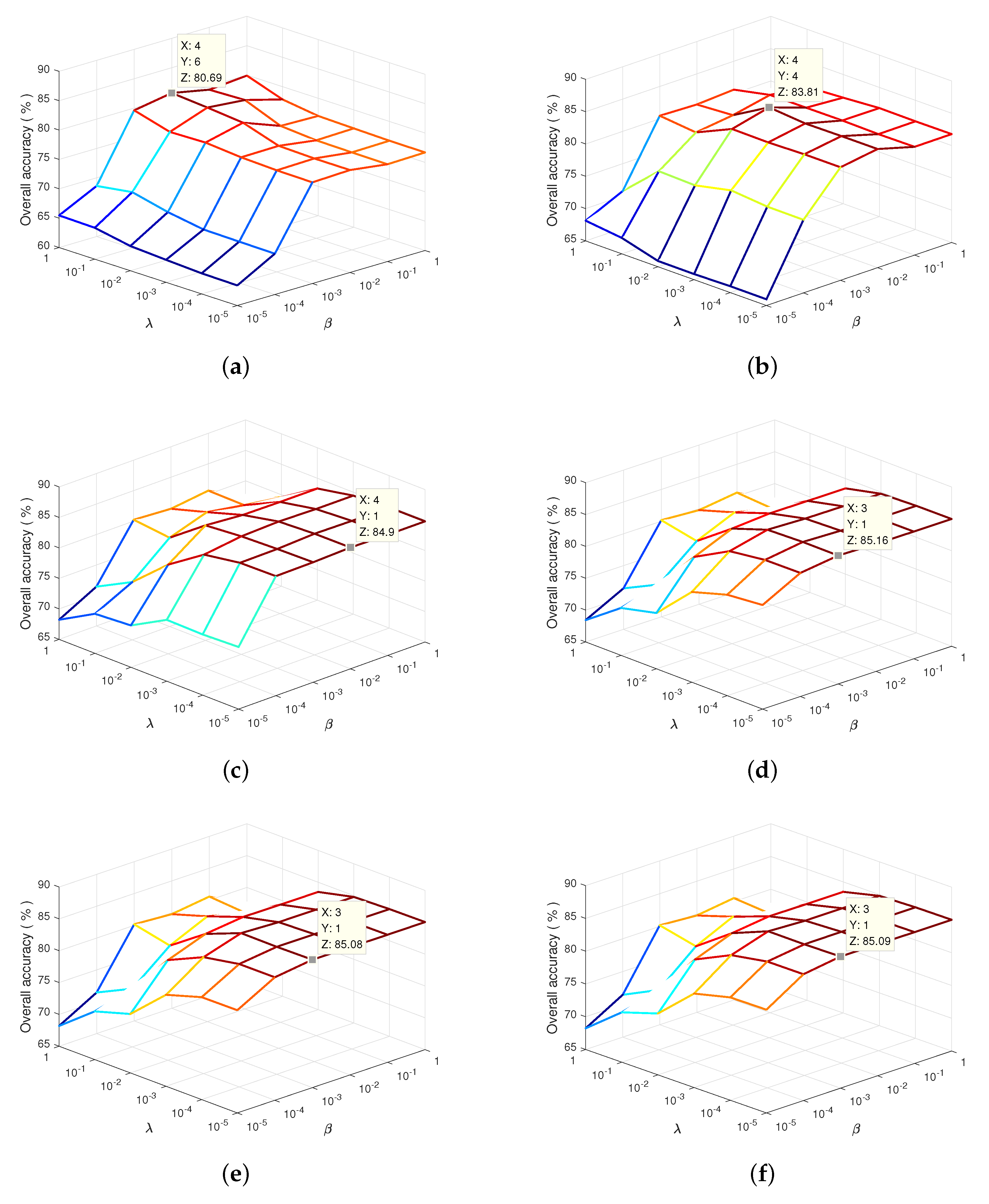
4.2. Analysis of the Regularization Parameters

From the proposed LatLRPL model, it can be directly seen that three regularization parameters $\lambda$, $\beta$, and $\gamma$ play an important role in balancing the contributions of different regularization terms. As such, these three parameters are tuned meticulously, in which the search range is set as {${10}^{-5},{10}^{-4},{10}^{-3},{10}^{-2},{10}^{-1},1$}. Figure 2 and Figure 3 show the variation of the performance with different $\lambda$, $\beta$, and $\gamma$ for the Indian Pines and the Pavia University datasets, respectively. To make it clear for observation, the best performance is marked in each figure. After comparison, [${10}^{-3},{10}^{-3},{10}^{-1}$] is confirmed for the Indian Pines dataset, and [${10}^{-5},{10}^{-3},{10}^{-3}$] is suitable for the Pavia University dataset.

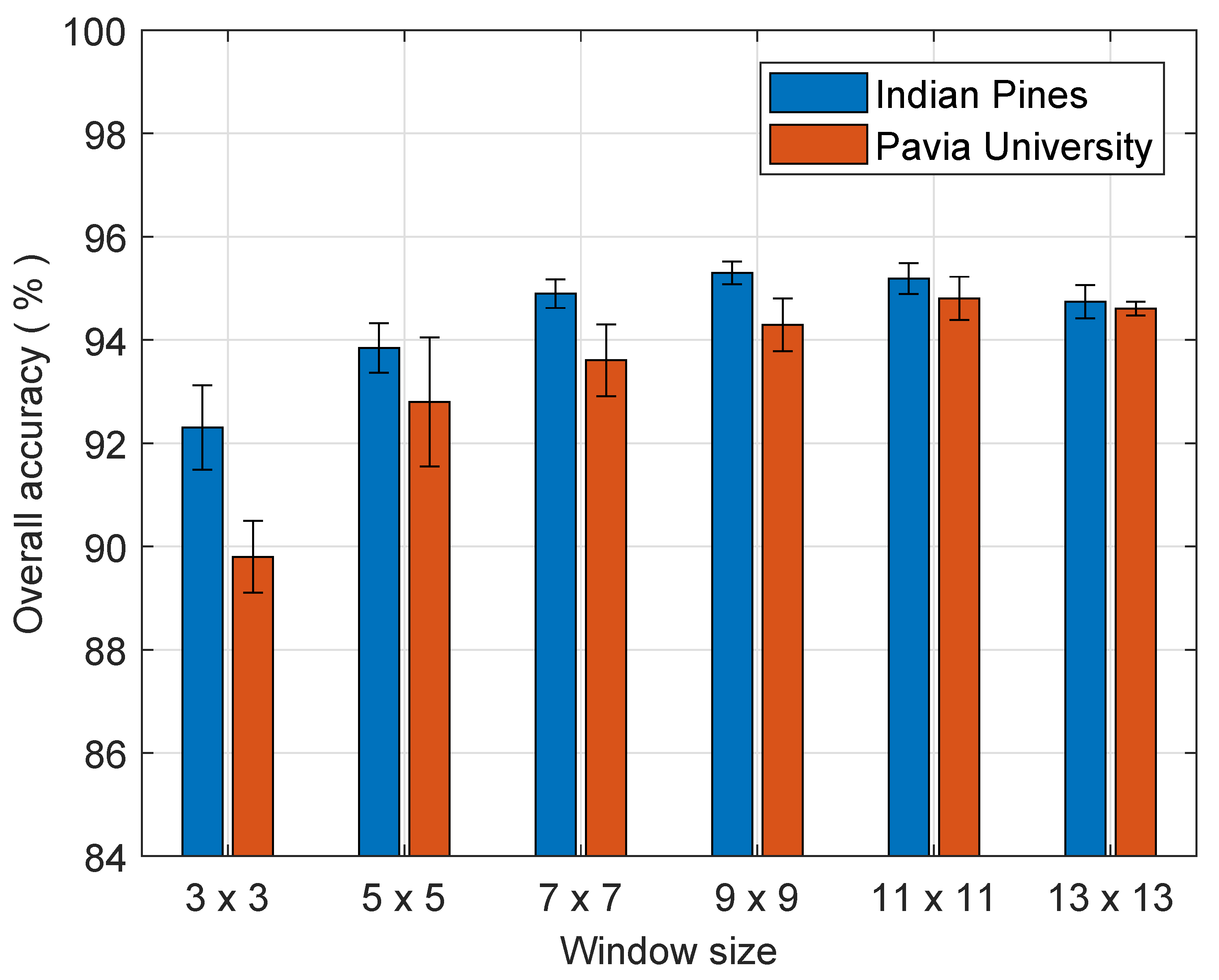
4.3. Analysis of the Sliding Window Size

For the proposed SpaLatLRPL method, the quality of data preprocessing is determined by the size of the sliding window. According to previous researches, the neighborhood size is searched from the range of $\{3\times 3,5\times 5,7\times 7,9\times 9,11\times 11,13\times 13\}$, whose results are shown in Figure 4 for the Indian Pines and the Pavia University datasets. Obviously, SpaLatLRPL can obtain the best performance when the window size is fixed at $9\times 9$ and $11\times 11$ for the two HSI datasets, respectively. Specifically, due to a much larger scene and significantly fewer categories presented in the Pavia University dataset than those in the Indian Pines dataset, a little larger neighborhood size is more suitable.

4.4. Analysis of the Number of Features

For feature extraction methods, the number of preserved features is still a problem of concern. Figure 5 shows the performance variation with different numbers of features for all compared methods, from which we can observe that the performance improves quickly with the number of features increasing and remains almost stable when the number of features achieves a certain value. To conduct a better comparison of the performance, the number of features is set as 30 for all considered methods in both datasets.

4.5. Comparison of the Classification Performance

Table 1. The comparison of performance for all methods on the Indian Pines dataset.

Class	LPP	NPE	SGE	LRGE	LatLRPL	MPCA	TLPP	SpaLatLRPL
1	39.59	37.55	42.45	33.06	29.80	59.18	90.48	66.67
	± 16.2	± 12.6	± 13.1	± 4.87	± 16.2	± 5.40	± 9.43	± 8.25
2	75.83	79.95	79.36	82.08	83.41	93.21	89.88	94.45
	± 1.82	± 2.24	± 1.56	± 0.99	± 2.06	± 1.39	± 1.93	± 0.74
3	64.61	67.06	66.79	70.39	77.20	93.96	83.89	95.83
	± 3.00	± 2.82	± 4.51	± 2.15	± 2.81	± 0.27	± 5.86	± 0.70
4	52.70	57.35	53.93	53.93	50.71	84.68	89.89	86.73
	± 9.30	± 6.72	± 6.93	± 8.71	± 9.33	± 7.29	± 6.00	± 9.25
5	92.98	92.53	93.42	92.66	91.81	94.71	95.82	97.39
	± 3.21	± 2.76	± 3.22	± 3.68	± 4.33	± 1.37	± 3.48	± 1.06
6	95.39	96.49	96.19	95.62	94.88	97.67	98.46	97.57
	± 1.55	± 1.27	± 1.48	± 1.20	± 1.22	± 1.08	± 0.56	± 0.73
7	20.00	13.04	31.30	6.08	38.26	0.00	55.07	0.00
	± 22.1	± 13.4	± 29.1	± 8.48	± 24.9	± 0.00	± 6.64	± 0.00
8	99.27	99.36	99.45	99.23	98.27	97.35	99.92	98.33
	± 0.41	± 0.19	± 0.20	± 0.59	± 1.77	± 1.74	± 0.13	± 0.65
9	3.33	0.00	4.44	0.00	8.88	1.85	33.33	11.11
	± 7.45	± 0.00	± 6.09	± 0.00	± 12.2	± 3.21	± 24.2	± 19.2
10	58.05	62.80	60.32	63.51	77.57	88.94	89.55	93.61
	± 3.02	± 5.24	± 6.38	± 4.03	± 2.60	± 1.35	± 1.92	± 0.43
11	80.87	82.97	82.35	87.28	89.30	95.02	92.65	97.63
	± 2.78	± 0.60	± 1.28	± 1.62	± 1.52	± 0.61	± 1.50	± 0.60
12	77.07	79.46	80.83	85.06	85.75	87.22	87.10	92.77
	± 2.89	± 1.68	± 4.72	± 2.28	± 2.94	± 5.27	± 4.76	± 2.20
13	98.32	97.91	98.43	98.12	94.87	96.16	97.21	95.29
	± 0.77	± 1.39	± 0.97	± 1.32	± 0.86	± 2.69	± 1.98	± 2.40
14	96.21	95.93	96.64	97.65	96.07	96.31	99.43	98.43
	± 2.47	± 3.05	± 2.33	± 0.90	± 1.17	± 1.12	± 0.84	± 0.13
15	57.66	57.43	60.76	54.74	57.43	85.19	91.91	92.11
	± 4.27	± 5.50	± 4.92	± 0.95	± 6.42	± 4.69	± 2.21	± 5.87
16	82.59	80.47	83.29	83.06	87.53	80.39	84.31	87.45
	± 8.74	± 9.58	± 7.64	± 6.31	± 8.71	± 13.2	± 5.43	± 8.76
OA	79.29	81.20	81.07	83.15	85.46	92.79	92.41	95.34
	± 0.65	± 0.72	± 0.73	± 0.51	± 0.58	± 0.51	± 1.01	± 0.22
AA	68.40	68.77	70.62	68.90	72.61	78.24	86.18	81.58
	± 1.18	± 0.47	± 2.06	± 0.46	± 2.01	± 0.85	± 0.59	± 0.74
$\kappa$	76.25	78.46	78.30	80.65	83.36	91.77	91.35	94.68
	± 0.68	± 0.83	± 0.89	± 0.60	± 0.67	± 0.58	± 1.16	± 0.33

and

Table 2. The comparison of performance for all methods on the Pavia University dataset.

Class	LPP	NPE	SGE	LRGE	LatLRPL	MPCA	TLPP	SpaLatLRPL
1	81.75	83.528	83.13	84.05	85.99	92.75	93.80	95.54
	± 4.30	± 2.9	± 3.46	± 2.95	± 4.33	± 1.06	± 0.55	± 3.63
2	94.21	95.05	94.52	95.26	96.47	97.86	95.65	99.40
	± 1.34	± 0.54	± 1.06	± 1.82	± 1.23	± 0.60	± 1.14	± 0.14
3	37.39	39.73	53.90	48.79	49.72	75.22	75.38	77.90
	± 12.2	± 19.9	± 6.78	± 7.13	± 11.1	± 3.16	± 4.00	± 4.93
4	82.34	77.74	79.79	77.42	81.64	87.58	91.84	91.92
	± 3.54	± 3.84	± 5.43	± 2.76	± 2.41	± 2.67	± 2.41	± 1.84
5	99.22	99.14	99.20	98.02	99.07	99.13	99.98	99.27
	± 0.54	± 0.50	± 0.69	± 1.72	± 0.62	± 0.81	± 0.03	± 0.75
6	51.97	55.59	55.79	58.05	60.92	77.55	72.93	93.39
	± 4.58	± 3.78	± 2.87	± 3.46	± 5.71	± 3.78	± 3.61	± 1.73
7	36.28	40.35	43.95	61.47	57.48	81.96	67.49	92.28
	± 8.19	± 9.21	± 6.51	± 3.87	± 9.14	± 7.08	± 9.61	± 1.60
8	70.95	73.48	72.34	80.71	84.47	87.19	80.52	84.57
	± 7.86	± 10.8	± 2.81	± 3.01	± 3.91	± 2.22	± 3.01	± 3.34
9	73.39	80.26	63.77	98.76	93.26	97.89	88.93	92.00
	± 7.60	± 11.4	± 34.4	± 2.20	± 4.23	± 1.14	± 4.59	± 1.29
OA	79.57	80.91	81.14	83.45	85.07	91.46	89.23	94.84
	± 0.94	± 0.99	± 0.76	± 0.90	± 0.80	± 0.56	± 0.97	± 0.34
AA	69.72	71.65	71.82	78.06	78.78	88.57	85.17	91.81
	± 1.68	± 2.41	± 4.09	± 0.31	± 1.59	± 0.60	± 0.87	± 0.61
$\kappa$	72.32	74.08	74.46	77.63	79.81	88.56	85.61	93.13
	± 1.22	± 1.39	± 1.13	± 1.12	± 1.06	± 0.76	± 1.29	± 0.66

present the class-specific accuracy, OA, AA, and $\kappa$ coefficient for all compared methods by conducting the experiments on the two HSI datasets. Specifically, 10% samples randomly selected from the total samples are used to train the SVM classifier, and the rest of the samples are utilized for testing in the Indian Pines dataset, while the percentage of training samples in the Pavia University dataset utilized for training is 1%. From Table 1, the proposed unsupervised LatLRPL method performs best among all the spectral-based feature extraction methods, presenting at least two percent gain when compared with that of LPP [21], NPE [23], SGE [29], and LRGE [35]. Specifically, LPP, NPE, SGE, and LRGE construct the neighborhood graph depending on the nearest distance or the largest representative coefficients, and the inaccuracy of the graph may lead to the error propagation to low-dimensional projection, which can degrade the discriminant ability of the extracted features. To be different, the proposed LatLRPL method learns the projection matrix in an integrated latent low-rank representation model, which is available to capture the intrinsic and discriminative features from the high-dimensional hyperspectral data.

For the comparison of spatial-spectral-based methods, the proposed SpaLatLRPL method also shows a great improvement in the performance, obtaining an almost three-point gain when compared with that of MPCA and TLPP. Specifically, SpaLatLRPL presents good results in similar classes, such as class 10, class 11, and class 12. However, SpaLatLRPL performs not well in small classes, such as class 7 and class 9, which may be the reason that the neighborhood size adopted in the weighted average strategy is not proper for small classes. To overcome this problem, an adaptive neighborhood size may work well. By comparing the performance of the spectral-based methods and the spatial-spectral-based methods, we can observe that the improvement is prominent, indicating that the spatial information is very beneficial for the feature extraction and classification task of HSIs. From Table 2, it can also be seen that the spatial-spectral-based methods perform much better than spectral-based methods in the Pavia University dataset, illustrating the importance of the spatial information. Overall, our proposed methods (LatLRPL and SpaLatLRPL) show great effectiveness in the feature extraction of HSIs, which also demonstrates that the spectral constraint and the graph regularization imposed on the original space and the low-dimensional space can improve the ability of the proposed methods in capturing local intrinsic structure, and in addition, the integrated projection learning framework is robust to noise.

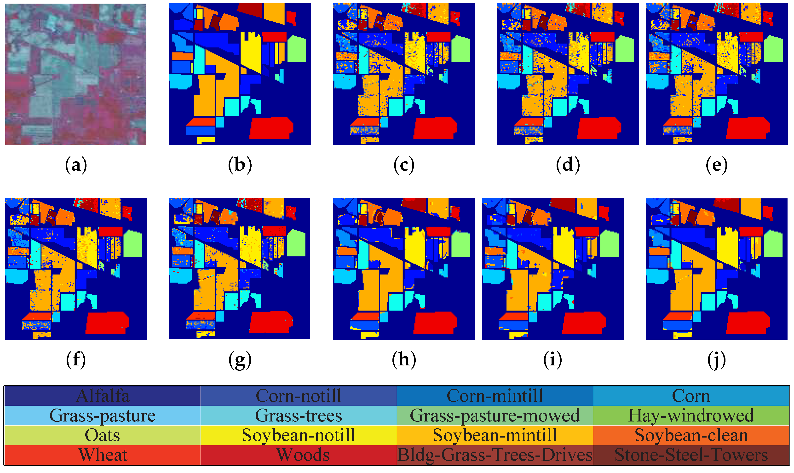
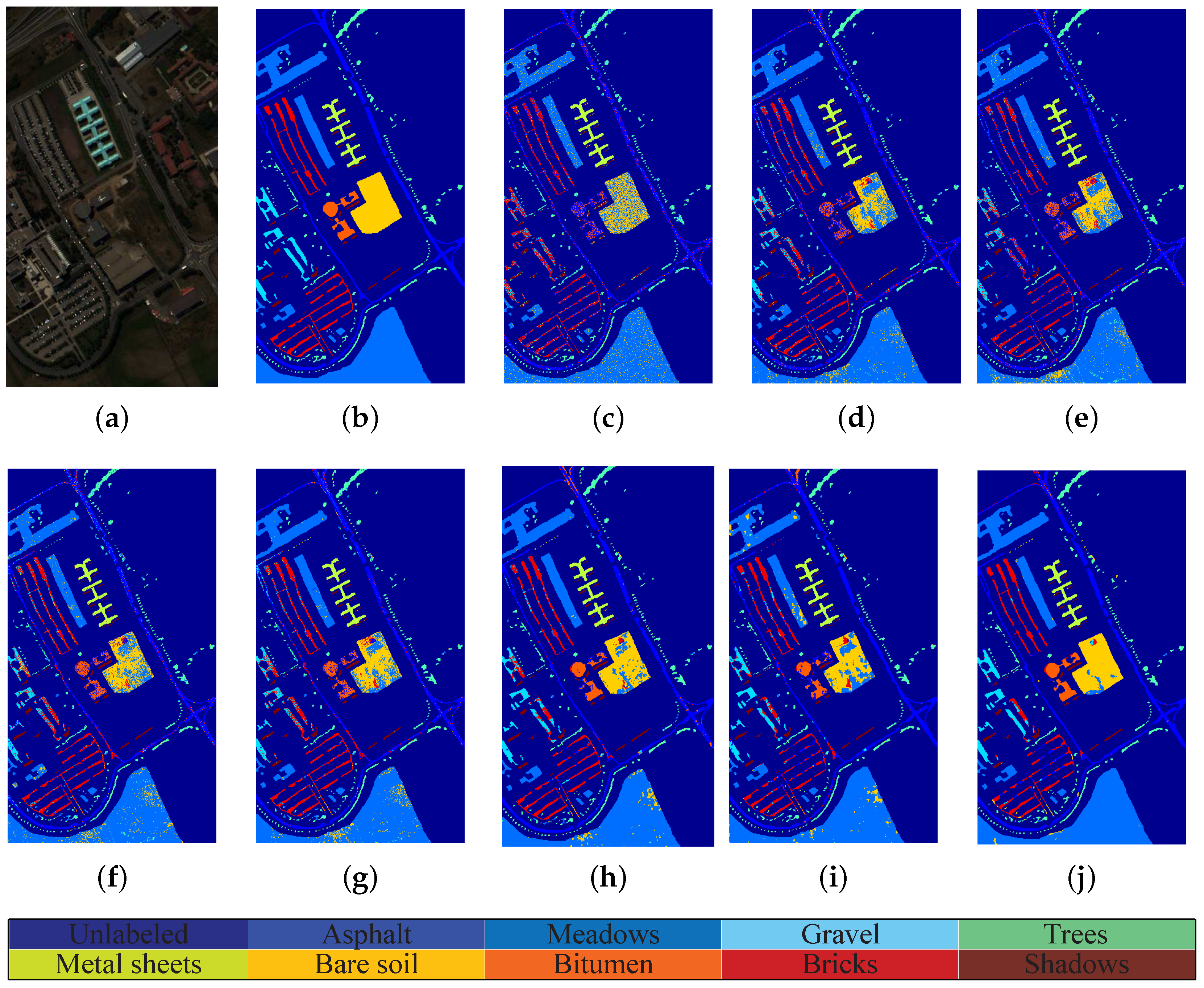
4.6. Presentation of Classification Maps

To present the performance of different feature extraction methods more directly, the classification maps are shown in Figure 6 and Figure 7, corresponding to the results given in Table 1 and Table 2 for the two datasets, respectively. Taking a close look at these figures, we can see that spatial-spectral-based methods obtain much smoother classification results, among which SpaLatLRPL shows the best classification performance, especially for the regions of “Soybean-notill”, “Soybean-mintill”, and “Soybean-clean” in the Indian Pines dataset and “Grave” and “Bare soil” in the Pavia University dataset. In addition, for spectral-based feature extraction methods, the proposed unsupervised LatLRPL method performs better than other considered methods. The classification maps illustrate the superiority of the proposed latent low-rank projection learning methods.

5. Conclusions

In this paper, a novel unsupervised feature extraction method, i.e., latent low-rank projection learning with graph regularization (LatLRPL), has been proposed for the feature extraction and classification of HSIs. To obtain the discriminative features with arbitrary dimensionality, the latent low-rank matrix mentioned in the latent low-rank representation is first decomposed into two different matrices, one of which can be exploited as the projection matrix. To better preserve the local intrinsic structure, regularization on the original space and the learned low-dimensional space is integrated into LatLRPL by making use of spectral constraints and graph regularization, thus forming a more discriminative feature extraction model. Different from the graph embedding-based methods that require two steps to obtain the projection matrix, the proposed LatLRPL method can deal with this in one model. In order to take advantage of spatial information in HSIs, a local weighted average strategy is adopted by computing the value of a central pixel with its neighboring pixels in a sliding window, followed by conducting LatLRPL on this new data. Experiments on two HSI datasets have demonstrated that the proposed LatLRPL method and its extension, SpaLatLRPL, perform better than all compared feature extraction methods.

References

1. Ghamisi, P.; Yokoya, N.; Li, J.; Liao, W.; Liu, S.; Plaza, J.; Rasti, B.; Plaza, A. Advances in hyperspectral image and signal processing: A comprehensive overview of the state of the art. IEEE Geosci. Remote Sens. Mag. 2017, 5, 37–78. [Google Scholar] [CrossRef] [Green Version]
2. Wen, J.; Fowler, J.E.; He, M.; Zhao, Y.Q.; Deng, C.; Menon, V. Orthogonal nonnegative matrix factorization combining multiple features for spectral-spatial dimensionality reduction of hyperspectral imagery. IEEE Trans. Geosci. Remote Sens. 2016, 54, 4272–4286. [Google Scholar] [CrossRef]
3. An, J.L.; Zhang, X.R.; Zhou, H.Y.; Jiao, L.C. Tensor-based low-rank graph with multimanifold regularization for dimensionality reduction of hyperspectral images. IEEE Trans. Geosci. Remote Sens. 2018, 56, 4731–4746. [Google Scholar] [CrossRef]
4. Sun, W.W.; Du, Q. Hyperspectral band selection: A review. IEEE Geosci. Remote Sens. Mag. 2019, 7, 118–139. [Google Scholar] [CrossRef]
5. Feng, J.; Feng, X.L.; Chen, J.T.; Cao, X.H.; Zhang, X.R.; Jiao, L.C.; Yu, T. Generative adversarial networks based on collaborative learning and attention mechanism for hyperspectral image classification. Remote Sens. 2020, 12, 1149. [Google Scholar] [CrossRef] [Green Version]
6. Feng, J.; Wu, X.D.; Shang, R.H.; Sui, C.H.; Li, J.; Jiao, L.C. Attention multibranch convolutional neural network for hyperspectral image classification based on adaptive region search. IEEE Trans. Geosci. Remote Sens. 2020, 59, 5054–5070. [Google Scholar] [CrossRef]
7. Yang, L.X.; Zhang, R.; Yang, S.Y.; Jiao, L.C. Hyperspectral Image Classification via Slice Sparse Coding Tensor Based Classifier With Compressive Dimensionality Reduction. IEEE Access 2020, 8, 145207–145215. [Google Scholar] [CrossRef]
8. Hang, R.L.; Liu, Q.S.; Sun, Y.B.; Yuan, X.T.; Pei, H.C.; Plaza, J.; Plaza, A. Robust matrix discriminative analysis for feature extraction from hyperspectral images. IEEE J. Sel. Top. Appl. Earth Observ. Remote Sens. 2017, 10, 2002–2011. [Google Scholar] [CrossRef]
9. Varga, D. Multi-pooled inception features for no-reference image quality assessment. Appl. Sci. 2020, 10, 2186. [Google Scholar] [CrossRef] [Green Version]
10. Varga, D. No-reference video quality assessment using multi-pooled, saliency weighted deep features and decision fusion. Sensors 2022, 22, 2209. [Google Scholar] [CrossRef]
11. Lin, C.Z.; Lu, J.W.; Wang, G.; Zhou, J. Graininess-aware deep feature learning for pedestrian detection. IEEE Trans. Image Process. 2020, 29, 3820–3834. [Google Scholar] [CrossRef] [PubMed]
12. Sethy, P.K.; Barpanda, N.K.; Rath, A.K.; Behera, S.K. Deep feature based rice leaf disease identification using support vector machine. Comput. Electron. Agric. 2020, 175, 105527. [Google Scholar] [CrossRef]
13. Zhang, W.B.; Zhang, L.M.; Pfoser, D.; Zhao, L. Disentangled dynamic graph deep generation. arXiv 2020, arXiv:2010.07276. [Google Scholar]
14. Jia, S.; Liao, J.H.; Xu, M.; Li, Y.; Zhu, J.S.; Sun, W.W.; Jia, X.P.; Li, Q.Q. 3-D gabor convolutional neural network for hyperspectral image classification. IEEE Trans. Geosci. Remote Sens. 2022, 60, 5509216. [Google Scholar] [CrossRef]
15. Wan, S.; Pan, S.R.; Zhong, P.; Chang, X.J.; Yang, J.; Gong, C. Dual interactive graph convolutional networks for hyperspectral image classification. IEEE Trans. Geosci. Remote Sens. 2022, 60, 5510214. [Google Scholar] [CrossRef]
16. Jolliffe, I.T. Principal Component Analysis; Springer: New York, NY, USA, 2002. [Google Scholar]
17. Bandos, T.V.; Bruzzone, L.; Camps-Valls, G. Classification of hyperspectral images with regularized linear discriminant analysis. IEEE Trans. Geosci. Remote Sens. 2009, 47, 862–873. [Google Scholar] [CrossRef]
18. Sugiyama, M. Dimensionality reduction of multimodal labeled data by local fisher discriminant analysis. J. Mach. Learn. Res. 2007, 8, 1027–1061. [Google Scholar]
19. Ma, L.; Crawford, M.M.; Yang, X.Q.; Guo, Y. Local-mainfold-learning-based graph construction for semisupervised hyperspectral image classification. IEEE Trans. Geosci. Remote Sens. 2015, 53, 2832–2844. [Google Scholar] [CrossRef]
20. Liao, D.P.; Qian, Y.T.; Tang, Y.Y. Constrained manifolding learning for hyperspectral imagery visualization. IEEE J. Sel. Top. Appl. Earth Observ. Remote Sens. 2017, 11, 1213–1226. [Google Scholar] [CrossRef] [Green Version]
21. He, X.F.; Niyogi, P. Locality preserving projections. In Proceedings of the 17th Annual Conference on Neural Information Processing Systems (NIPS 2003), Vancouver, BC, Canada, 8–13 December 2003; pp. 234–241. [Google Scholar]
22. Roweis, S.T.; Saul, L.K. Nonlinear dimensionality reduction by locally linear embedding. Science 2000, 290, 2323–2326. [Google Scholar] [CrossRef] [Green Version]
23. He, X.F.; Cai, D.; Yan, S.C.; Zhang, H.J. Neighborhood preserving embedding. In Proceedings of the Tenth IEEE International Conference on Computer Vision (ICCV’05), Beijing, China, 17–21 October 2005; pp. 1208–1213. [Google Scholar]
24. Belkin, M.; Niyogi, P. Laplacian eigenmaps for dimensionality reduction and data representation. Neural Comput. 2003, 15, 1373–1396. [Google Scholar] [CrossRef] [Green Version]
25. Yan, S.C.; Xu, D.; Zhang, B.Y.; Zhang, H.-J.; Yang, Q.; Lin, S. Graph embedding and extensions:a general framework for dimensionality reduction. IEEE Trans. Pattern Anal. Mach. Intell. 2007, 29, 40–51. [Google Scholar] [CrossRef] [PubMed] [Green Version]
26. Wright, J.; Yang, A.Y.; Ganesh, A.; Sastry, S.S.; Ma, Y. Robust face recognition via sparse representation. IEEE Trans. Pattern Anal. Mach. Intell. 2009, 31, 210–227. [Google Scholar] [CrossRef] [PubMed] [Green Version]
27. Peng, J.T.; Li, L.Q.; Tang, Y.Y. Maximum likelihood estimation based joint sparse representation for the classification of hyperspectral remote sensing images. IEEE Trans. Neural Netw. Learn. Syst. 2019, 30, 1790–1802. [Google Scholar] [CrossRef] [PubMed]
28. Gu, Y.F.; Wang, Y.T.; Zheng, H.; Hu, Y. Hyperspectral target detection via exploiting spatial-spectral joint sparsity. Neurocomputing 2015, 169, 5–12. [Google Scholar] [CrossRef]
29. Cheng, B.; Yang, J.C.; Yan, S.C.; Fu, Y.; Huang, T.S. Learning with l1-graph for image analysis. IEEE Trans. Image Process. 2015, 23, 2241–2253. [Google Scholar]
30. Qiao, L.S.; Chen, S.C.; Tan, X.Y. Sparsity preserving projections with applications to face recognition. Pattern Recognit. 2010, 43, 331–341. [Google Scholar] [CrossRef] [Green Version]
31. Ly, N.H.; Du, Q.; Fowler, J.E. Sparse graph-based discriminant analysis for hyperspectral imagery. IEEE Trans. Geosci. Remote Sens. 2014, 52, 3872–3884. [Google Scholar]
32. He, W.; Zhang, H.Y.; Zhang, L.P.; Philips, W.; Liao, W.Z. Weighted sparse graph based dimensionality reduction for hyperspectral images. IEEE Geosci. Remote Sens. Lett. 2016, 13, 686–690. [Google Scholar] [CrossRef] [Green Version]
33. Ly, N.H.; Du, Q.; Fowler, J.E. Collaborative graph-based discriminant analysis for hyperspectral imagery. IEEE J. Sel. Top. Appl. Earth Observ. Remote Sens. 2014, 7, 2688–2696. [Google Scholar] [CrossRef]
34. Zhang, L.; Yang, M.; Feng, X.H. Sparse representation or collaborative representation: Which helps face recognition? In Proceedings of the 2011 International Conference on Computer Vision, Barcelona, Spain, 6–13 November 2011. [Google Scholar]
35. Liu, G.C.; Lin, Z.C.; Yan, S.C.; Sun, J.; Yu, Y.; Ma, Y. Robust recovery of subspace structure by low-rank representation. IEEE Trans. Pattern Anal. Mach. Intell. 2013, 35, 171–184. [Google Scholar] [CrossRef] [PubMed] [Green Version]
36. Zhuang, L.S.; Gao, S.H.; Tang, J.H.; Wang, J.J.; Lin, Z.C.; Ma, Y.; Yu, N.H. Constructing a nonnegative low-rank and sparse graph with data-adaptive features. IEEE Trans. Image Process. 2015, 24, 3717–3728. [Google Scholar] [CrossRef] [PubMed] [Green Version]
37. de Morsier, F.; Borgeaud, M.; Gass, V.; Thiran, J.-P.; Tuia, D. Kernel low-rank and sparse graph for unsupervised and semi-supervised classification of hyperspectral images. IEEE Trans. Geosci. Remote Sens. 2016, 54, 3410–3420. [Google Scholar] [CrossRef]
38. Li, W.; Liu, J.B.; Du, Q. Sparse and low-rank graph for discriminant analysis of hyperspectral imagery. IEEE Trans. Geosci. Remote Sens. 2016, 54, 4094–4105. [Google Scholar] [CrossRef]
39. Pan, L.; Li, H.-C.; Li, W.; Chen, X.-D.; Wu, G.-N.; Du, Q. Discriminant analysis of hyperspectral imagery using fast kernel sparse and low-rank graph. IEEE Trans. Geosci. Remote Sens. 2017, 55, 6085–6098. [Google Scholar] [CrossRef]
40. Pan, L.; Li, H.-C.; Deng, Y.J.; Zhang, F.; Chen, X.-D.; Du, Q. Hyperspectral dimensionality reduction by tensor sparse and low-rank graph-based discriminant analysis. Remote Sens. 2017, 9, 452. [Google Scholar] [CrossRef] [Green Version]
41. Mei, S.H.; Bi, Q.Q.; Ji, J.Y.; Hou, J.H.; Du, Q. Hyperspectral image classification by exploring low-rank property in spectral or/and spatial domain. IEEE J. Sel. Top. Appl. Earth Observ. Remote Sens. 2017, 10, 2910–2921. [Google Scholar] [CrossRef]
42. He, W.; Zhang, H.Y.; Zhang, L.P.; Shen, H.F. Total-variation-regularized low-rank matrix factorization for hyperspectral image restoration. IEEE Trans. Geosci. Remote Sens. 2016, 54, 178–188. [Google Scholar] [CrossRef]
43. Xue, J.Z.; Zhao, Y.Q.; Liao, W.Z.; Kong, S.G. Joint Spatial and Spectral Low-Rank Regularization for Hyperspectral Image Denoising. IEEE Trans. Geosci. Remote Sens. 2018, 56, 1940–1958. [Google Scholar] [CrossRef]
44. Liu, G.C.; Yan, S.C. Latent low-rank representation for subspace segementation and feature extraction. In Proceedings of the 2011 International Conference on Computer Vision, Barcelona, Spain, 6–13 November 2011. [Google Scholar]
45. Pan, L.; Li, H.-C.; Sun, Y.-J.; Du, Q. Hyperspectral image reconstruction by latent low-rank representation for classification. IEEE Geosci. Remote Sens. Lett. 2018, 15, 1422–1426. [Google Scholar] [CrossRef]
46. Fang, X.Z.; Han, N.; Wu, J.G.; Xu, Y. Approximate low-rank projection learning for feature extraction. IEEE Trans. Neural Netw. Learn. Syst. 2018, 29, 5228–5241. [Google Scholar] [CrossRef] [PubMed]
47. Pan, L.; Li, H.-C.; Meng, H.; Li, W.; Du, Q.; Emery, W.J. Hyperspectral image classification via low-rank and sparse representation with spectral consistency constraint. IEEE Geosci. Remote Sens. Lett. 2017, 14, 2117–2121. [Google Scholar] [CrossRef]
48. Boyd, S.; Parikh, N.; Chu, E.; Peleato, B.; Eckstein, J. Distributed optimization and statistical learning via the alternating direction method of multipliers. Found. Trends Mach. Learn. 2011, 3, 1–122. [Google Scholar] [CrossRef]
49. Cai, J.-F.; Candés, E.J.; Shen, Z. A singular value thresholding algorithm for matrix completion. SIAM J. Optim. 2010, 24, 1956–1982. [Google Scholar] [CrossRef]
50. Zou, H.; Hastie, T.; Tibshirani, R. Sparse principle component analysis. J. Comput. Graph. Stat. 2006, 15, 265–286. [Google Scholar] [CrossRef] [Green Version]
Figure 1. The framework of the proposed LatLRPL method.
Remotesensing 14 03078 g001
Figure 2. Parameter analysis of β , λ with different γ for the Indian Pines data: (a) γ = 1 , (b) γ = 0.1 , (c) γ = 0.01 , (d) γ = 0.001 , (e) γ = 0.0001 , (f) γ = 0.00001 .
Remotesensing 14 03078 g002
Figure 3. Parameter analysis of β , λ with different γ for the Pavia University data: (a) γ = 1 , (b) γ = 0.1 , (c) γ = 0.01 , (d) γ = 0.001 , (e) γ = 0.0001 , (f) γ = 0.00001 .
Remotesensing 14 03078 g003
Figure 4. Parameter analysis of window size for two datasets.
Remotesensing 14 03078 g004
Figure 5. Parameter analysis of the number of preserved features: (a) Indian Pines, (b) Pavia University.
Remotesensing 14 03078 g005
Figure 6. Classification maps of different methods for the Indian Pines dataset: (a) Pseudocolor image, (b) ground truth, (c) LPP, (d) NPE, (e) SGE, (f) LRGE, (g) LatLRPL, (h) MPCA, (i) TLPP, (j) SpaLatLRPL.
Remotesensing 14 03078 g006
Figure 7. Classification maps of different methods for the Pavia University dataset: (a) Pseudocolor image, (b) ground truth, (c) LPP, (d) NPE, (e) SGE, (f) LRGE, (g) LatLRPL, (h) MPCA, (i) TLPP, (j) SpaLatLRPL.
Remotesensing 14 03078 g007