Prediction of Total Phosphorus Concentration in Macrophytic Lakes Using Chlorophyll-Sensitive Bands: A Case Study of Lake Baiyangdian

Abstract

Total phosphorus (TP) is a significant indicator of water eutrophication. As a typical macrophytic lake, Lake Baiyangdian is of considerable importance to the North China Plain’s ecosystem. However, the lake’s eutrophication is severe, threatening the local ecological environment. The correlation between chlorophyll and TP provides a mechanism for TP prediction. In view of the absorption and reflection characteristics of the chlorophyll concentrations in inland water, we propose a method to predict TP concentration in a macrophytic lake with spectral characteristics dominated by chlorophyll. In this study, water spectra noise is removed by discrete wavelet transform (DWT), and chlorophyll-sensitive bands are selected by gray correlation analysis (GRA). To verify the effectiveness of the chlorophyll-sensitive bands for TP concentration prediction, three different machine learning (ML) algorithms were used to build prediction models, including partial least squares (PLS), random forest (RF) and adaptive boosting (AdaBoost). The results indicate that the PLS model performs well in terms of TP concentration prediction, with the least time consumption: the coefficient of determination (R²) and root mean square error (RMSE) are 0.821 and 0.028 mg/L in the training dataset, and 0.741 and 0.029 mg/L in the testing dataset, respectively. Compared with the empirical model, the method proposed herein considers the correlation between chlorophyll and TP concentration, as well as a higher accuracy. The results indicate that chlorophyll-sensitive bands are effective for predicting TP concentration.

1. Introduction

Lakes are vital freshwater resources on land, fulfilling several key ecological functions, such as providing water, purifying pollution, and maintaining biodiversity [1,2,3]. Owing to the influence of human activities and urbanization, many lakes face serious ecological problems, including reduced water volume, declining aquatic biodiversity, and water eutrophication. It is the premise and foundation of lake ecological environmental management that accurate and rapid monitoring of lake water quality [4,5].

Phosphorus is an essential element for algae growth, and the monitoring of total phosphorus (TP) is crucial for the monitoring and treating of water environments. However, high-precision TP concentration prediction remains challenging [6,7,8,9,10]. The existing in situ TP monitoring techniques are primarily based on the chemical method, which has the disadvantages of a long analysis period, chemical reagent consumption, and the generation of secondary pollution. In recent decades, remote sensing technology has been widely used to monitor the water quality of various inland lakes, due to its wide range of capabilities and timeliness [11,12,13,14]; it could serve as a new tool for the monitoring of TP concentration.

As an optically inactive substance, the TP concentration is difficult to invert using physical models [6,9]. The existing TP inversion models are broadly divided into direct and indirect models. The direct models establish the relationship between remote sensing reflectance (R_rs) and the measured TP concentration, and have been widely applied for water quality monitoring owing to their simplicity and feasibility. The direct models typically use statistical methods to estimate the water quality parameters with less consideration of the mechanism; therefore, these models’ applicability is limited, depending on the study area and data [7,8,9]. Chlorophyll-a, total suspended matter (TSM), and colored dissolved organic matter (CDOM) have optical properties and spectral responses, and TP concentration is correlated with the content of these optically active substances [6,15,16]. The indirect methods typically establish the relationship between the TP and optically active substances, and the TP concentration is subsequently indirectly retrieved, based on the inversion results of optically active substances [17]. Unlike the direct models, the indirect models consider the mechanism by which the TP is inverted. However, the inversion results of optically active substances, as well as the correlation between the TP and optically active substances, affect the accuracy of the TP inversion results. Earlier studies demonstrated a correlation between chlorophyll-a and TP, as well as total nitrogen (TN) [18,19,20,21,22,23], which provides a mechanism for TP concentration prediction through the chlorophyll-sensitive bands. Based on the spectral responses of emergent plants to different TN concentrations, Wang et al. and Liu et al. retrieved the concentration of TN through the sensitive bands of vegetation, using unmanned aerial vehicle (UAV) hyperspectral data for Ebinur Lake, and obtained high TN concentration prediction accuracy [24,25].

Machine learning (ML) is a branch of computer science that has been widely used for ecological and environmental remote sensing. Owing to their good computing performance and nonlinear mapping capabilities, ML models have increasingly been adopted as effective models for the inversion of water quality parameters in recent years, such as support vector machines (SVM), random forest (RF), genetic algorithms (GA), extreme learning machines (ELM), and artificial neural networks (ANN) [24,26,27,28,29,30]. Numerous researchers have analyzed the relationship between the water quality parameters and spectral data, using ML algorithms based on the measured water quality and spectral data, indicating that the ML algorithms may be capable of handling the nonlinear relationships between reflectance and water quality parameters [24,28,31].

Lake Baiyangdian is the largest freshwater wetland in the North China Plain, and the largest lake in Hebei Province [32,33,34]. It is a typical plant-dominated shallow freshwater lake; also a significant freshwater breeding base in northern China, with an extremely high ecological and economic status [35,36,37,38,39]. Lake Baiyangdian is also instrumental in maintaining the wetland ecosystem’s balance, regulating the climate, improving the temperature and humidity, replenishing the groundwater, and protecting biodiversity and rare species [40]. The presence of industrial wastewater, domestic sewage, and domestic waste has negatively impacted the ecological environment in some areas of Lake Baiyangdian [37,40,41], posing a considerable threat to the water environment’s security. Lake Baiyangdian is facing serious eutrophication, its water quality urgently requires monitoring, and several studies have used remote sensing technology to assess the lake’s water quality [32,33,42]. However, as an important indicator of water eutrophication, Lake Baiyangdian’s TP remains insufficiently investigated.

Consequently, the present study’s objectives are as follows: to explore the characteristic bands for TP inversion of inland lakes with chlorophyll-dominated spectral characteristics; to verify the effectiveness of the TP predictions based on chlorophyll-sensitive bands through different ML models; and to characterize the spatial distribution of water quality at sampling points across Lake Baiyangdian.

2. Materials and Methods

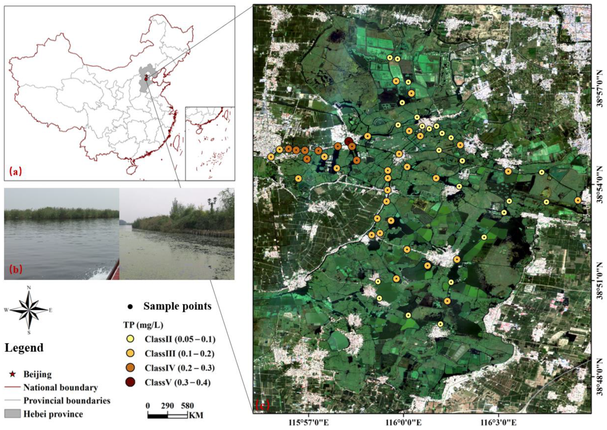
2.1. Study Area

Lake Baiyangdian is a freshwater lake in the Haihe River Basin, located at 38°43′–39°02′N and 115°45′–116°07′E in the Xiong’an New Area of Hebei Province, China (Figure 1). Lake Baiyangdian is composed of 143 lakes of various sizes with a total area of 366 square kilometers and an average annual water storage of 1.32 billion cubic meters. The river network in the basin shows a fan-shaped distribution [34,43]. The climate in the Lake Baiyangdian area is a typical temperate monsoon climate, with uneven distribution of precipitation throughout the year [36]. More of the precipitation occurs during the spring, and less in the autumn, while the precipitation between June and September accounts for 70–80% of the entire year’s rainfall [44]. The lake has a semi-arid climate: the drought index is 2.98, the annual average temperature is 7 °C, the average precipitation is 550 mm, and the annual average evaporation is 1637 mm [44,45].

Lake Baiyangdian is experiencing extreme water shortages. Its annual average water resource is 3.118 billion m³, and the per capita water resource is 297 m³—a mere 1/10 of the national per capita water resource. Owing to the occurrence of drying up incidents over the last 30 years, the amount of water entering Lake Baiyangdian has decreased [46]. At the same time, severe organic pollution and eutrophication affect most areas of the lake, and the main pollutants are chemical oxygen demand (COD) and TP derived from the rivers entering the lake from scenic spots and households [43,47,48,49]. Due to the domestic sewage and agricultural non-point source pollution in the lake area, Lake Baiyangdian’s water quality is poor (largely at the level of class IV–V) [46,48,50], and is deteriorating in some areas, posing a serious threat to the ecological environment. The situation of Lake Baiyangdian’s ecological environment is critical and must be addressed.

2.2. Data Acquisition

Figure 2 presents the study flowchart. The overall TP prediction framework comprises four steps, each of which is described in detail below. Owing to the rich spectral information, hyperspectral remote sensing can capture the water’s weak spectral characteristics and has been widely used in water quality monitoring [51,52,53,54,55]. In this study, a PSR-3500 portable spectrometer was used to measure the water spectra. The PSR-3500 is widely used for spectral measurement of ground objects. It has 1024 channels over a spectral range of 350–2500 nm, with spectral resolutions of 3.5, 10, and 7 nm at 700, 1500, and 2100 nm. A fiber optic probe with a field of view of 25° was used for the measurements.

The 62 sampling points were evenly distributed throughout the intersection and middle of the river in Lake Baiyangdian. The experiment was conducted on sunny days between 10:00 a.m. and 14:00 p.m., from 22 to 29 September 2018. For each sampling site, the radiances of water, sky, and the reference panel were measured, and water samples were collected simultaneously. Special observation geometry was adopted to avoid any influence of ships’ shadows and direct solar radiation [56]. All of the water samples were placed in the incubator and then brought to the chemical laboratory to test the TP concentration within 24 h. In this paper, the TP concentration was measured by the ammonium molybdate spectrophotometric method (GB 11893-1989, issued by China). To reduce the influence of random error, the spectra were measured five times at the same spot, and the final spectrum was determined from the average of the five spectra for each sample site. R_rs was derived, using the following Equation (1):

$$R_{rs}\left(\lambda \right)=\frac{L_{SW}-r{L}_{sky}}{L_p\ast \frac{\pi }{{\rho }_p}}$$

(1)

where $L_{SW}$ is the total radiance of the water; $L_{sky}$ is the measured radiance of the sky; $L_p$ is the measured radiance of the reference panel; ${\rho }_p$ is the reflectance of the reference panel (30%); and r is the skylight reflectance at the air–water surface.

2.3. Spectral Preprocessing

Spectral dimension noise distorts the spectrum of ground objects, shifts the central wavelength, and thus affects the inversion results of water quality parameters. Therefore, the removal of spectral dimension noise is critical to improve the accuracy of water quality parameters. Owing to its good time-frequency resolution characteristics, wavelet transform (WT) is widely used to remove noise from spectral data [57,58]. WT transforms the function in time and space to determine the relationship between the time and frequency domains, including continuous WT and discrete wavelet transform (DWT). For the discrete case, the wavelet sequence is defined as follows:

$${\Psi }_{j,k}\left(t\right)={\left|a_0\right|}^{-\frac{j}{2}}\Psi \left(a_0^{-j}t-k{\tau }_0\right)$$

(2)

where a and b are the zoom and translation factor, respectively; $a,b\in R;$ and $a\ne 0$. For any function f(t), the DWT is defined, using Equation (3):

$$W_f\left(j,k\right)=\langle f\left(t\right),{\Psi }_{j,k}\left(t\right)\rangle =a_0^{-\frac{j}{2}}{{\displaystyle \int }}_{-\infty }^{+\infty }f\left(t\right)\Psi \left(a_0^{-j}t-k{\tau }_0\right)dt$$

(3)

DWT decomposes the signal into detail and approximate coefficients. The signal S is decomposed into three layers, and the decomposition relation is, S = A₃ + D₃ + D₂ + D₁, as shown in Figure 3. A₃ is the approximate coefficient of the original signal, which is the low-frequency component; D₁–D₃ are the detail coefficients, which are the high-frequency components.

To evaluate the de-noising results, the normalized correlation coefficient (NCC), signal to noise ratio (SNR), and peak signal to noise ratio (PSNR) were calculated, using the following equations, respectively:

$$NCC=\frac{{{\displaystyle \sum }}_{i=1}^N{x}_i{\widehat{x}}_i}{\sqrt{\left[{{\displaystyle \sum }}_{i=1}^N{x}_i^2\right]·\left[{{\displaystyle \sum }}_{i=1}^N{\widehat{x}}_i{}^2\right]}}$$

(4)

$$SNR=10\times \lg \left[\frac{{{\displaystyle \sum }}_{i=1}^N{x}_i^2}{{{\displaystyle \sum }}_{i=1}^N{(x_i-{\widehat{x}}_i)}^2}\right]$$

(5)

$$PSNR=10\times \lg \left[\frac{{(x_i)}_{max}^2\times N}{{{\displaystyle \sum }}_{i=1}^N{(x_i-{\widehat{x}}_i)}^2}\right]$$

(6)

where N is the total number of samples; $x_i$ is the spectral reflectance before de-noising; and ${\widehat{x}}_i$ is the spectral reflectance after de-noising. The DWT de-noising method was performed using MATLAB R2017a.

2.4. Gray Relation Analysis

The degree of relevance reflects the relevance of two sequences. The grey relation analysis (GRA) is based on grey system theory, which reveals the characteristics and degree of the relationship between factors [59,60]. Owing to its characteristics, such as the lower sample size and calculation requirements, and the lack of need for typical distribution rules, GRA is widely used for nonlinear feature selection. As a dimensionless quantity, GRA can express the correlation between the TP concentration and hyperspectral reflectance of the water samples. A more detailed description of GRA is provided by Kuo et al. [61]. The GRA was written using Python 3.7.

2.5. Prediction Model Construction and Verification

To verify the effectiveness of predicting the TP concentration through the chlorophyll-sensitive bands, and to better understand the nonlinear relationship between TP concentration and reflectance, three typical ML algorithms were used in this paper, including partial least squares (PLS), random forest (RF), and adaptive boosting (AdaBoost).

(a)

Partial least squares

PLS is a typical parametric regression method, which has been widely used in studies owing to the good performance [62,63]. It is applicable to the case where the amount of highly collinear data and variables significantly exceeds the number of available samples. The PLS method selects successive orthogonal factors that maximize the covariance between the predictor and response variables to predict the variables. It takes advantage of the correlation between the TP concentration and reflectance spectra, and derives quantitative information from the spectra data.

(b)

Random forest

RF is a decision tree algorithm, based on ensemble learning algorithms. It has higher accuracy when used to solve nonlinear problems for regression and classification. As such, it has been widely used in remote sensing studies [64,65]. The RF algorithm uses multiple models when the samples are input, and the algorithm then integrates all of the models’ results to derive a single model. The performance of the RF models is usually evaluated based on the out-of-bag (OOB) error. A detailed illustration of the RF method is available in the paper of Genuer et al. [66].

(c)

Adaptive boosting

The AdaBoost algorithm is an integrated learning algorithm, based on the boosting algorithm framework. As an effective statistical learning algorithm, the AdaBoost algorithm is not susceptible to overfitting issues and is widely used in classification and regression problems [27,28,67,68]. It serially constructs a strong learner, with a weak learner that is continuously used to make up for the previous weak learner’s shortcomings. The training samples are weighted in each iteration, and the weight is adjusted according to the error [26]. When the weight of the learner with the larger error is reduced and the weight of the learner with the smaller error is increased, the final weighted set becomes a strong learner. AdaBoost is also an iterative optimal search strategy. By searching the learner or function space, it constructs a perfect learner to ensure a sufficiently small objective function.

To evaluate the predictions of the TP concentration, four parameters were calculated, namely the coefficient of determination (R²), root mean square error (RMSE), ratio of performance to deviation (RPD), and explained variance score (EVS). The RPD is the ratio between the standard deviation (SD) and the RMSE. These parameters were determined using Equations (7)–(10), respectively:

$$R^2=\frac{{{\displaystyle \sum }}_{i=1}^N{\left({\widehat{y}}_i-\overline{y}\right)}^2}{{{\displaystyle \sum }}_{i=1}^N{\left(y_i-\overline{y}\right)}^2}$$

(7)

$$RMSE=\sqrt{\frac{1}{N}{\displaystyle \sum }_{i=1}^N{\left(y_i-{\widehat{y}}_i\right)}^2}$$

(8)

$$RPD=\frac{SD}{RMSE}$$

(9)

$$EVS=1-\frac{Var\left\{y_i-{\widehat{y}}_i\right\}}{Var\left\{y_i\right\}}$$

(10)

where N is the total number of samples; ${\widehat{y}}_i$ is the predicted value; $y_i$ is the measured value; and $\overline{y}$ is the mean of the measured value. Generally, a robust model has a high R², RPD, and EVS, and a low RMSE. The PLS, RF, AdaBoost method, and four evaluating indicators were performed and implemented using Python 3.7.

3. Results

3.1. Statistical Analysis

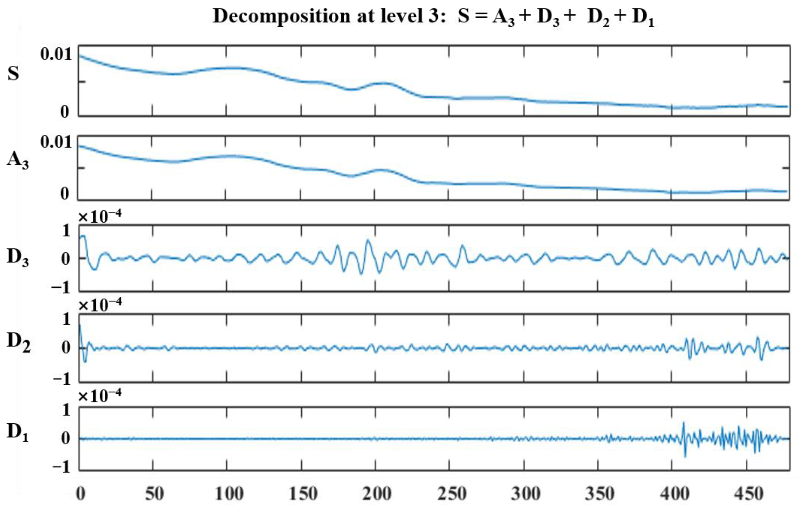
Based on the in situ data, the water samples were sorted, according to the TP concentration. Every third sample was included in the testing dataset; the rest of the data were included in the training dataset. The 62 water samples collected from Lake Baiyangdian were divided into 42 training datasets and 20 testing datasets. The training and testing datasets were representative of the entire water sample dataset in terms of the minimum, maximum, mean, and SD values. The coefficient of variation (CV) was used to complement the SD.

Table 1. TP concentrations (mg/L) of measured water samples in Lake Baiyangdian.

Group	Max	Min	Mean	SD	CV
Entire dataset (n = 62)	0.31	0.05	0.136	0.065	0.482
Training dataset (n = 42)	0.31	0.05	0.137	0.07	0.514
Testing dataset (n = 20)	0.27	0.07	0.134	0.055	0.413

presents the statistics for the water samples’ TP concentrations. The minimum TP concentration was 0.05 mg/L, and the maximum concentration was 0.31 mg/L.

3.2. DWT Denoising

In the DWT analysis, we decomposed the spectral data into three layers after several tests. The spectral de-noising filter, based on WT, includes hard and soft thresholds. In this paper, the detailed information of each layer is filtered by threshold selection, and the filtered spectra data are reconstructed by inverse WT.

Table 2. Comparison of the de-noising effects of different wavelet functions.

	Function	NCC	SNR (dB)	PSNR (dB)
Daubechies	db4	0.999986	45.6378	51.5475
	db5	0.999981	44.1852	50.0514
	db6	0.999979	43.7034	49.6225
Symlets	sym4	0.999978	43.5734	49.4839
	sym5	0.999978	43.5775	49.4516
	sym6	0.99998	43.9002	49.8099
Coiflet	coif3	0.999979	43.8615	49.7811
	coif4	0.999982	44.3825	50.2567
	coif5	0.999981	44.2161	50.0769

compares the de-noising effects among different mother wavelet functions (db, sym, and coif). NCC was used to evaluate the spectra before and after de-noising; SNR and PSNR were used to evaluate the information reconstruction quality of the spectra. Generally, the better the information quality of the spectra, the greater that of the NCC, SNR, and PSNR. As Table 2 illustrates, the NCC values show little difference between the different functions, demonstrating that good waveform similarity can be maintained after de-noising with different wavelet functions. The SNR and PSNR of the spectra de-noised by db4 were 45.6378 and 51.5475 dB, respectively—higher than those of the other wavelet functions. The water spectra de-noised by db4 are shown in Figure 4a.

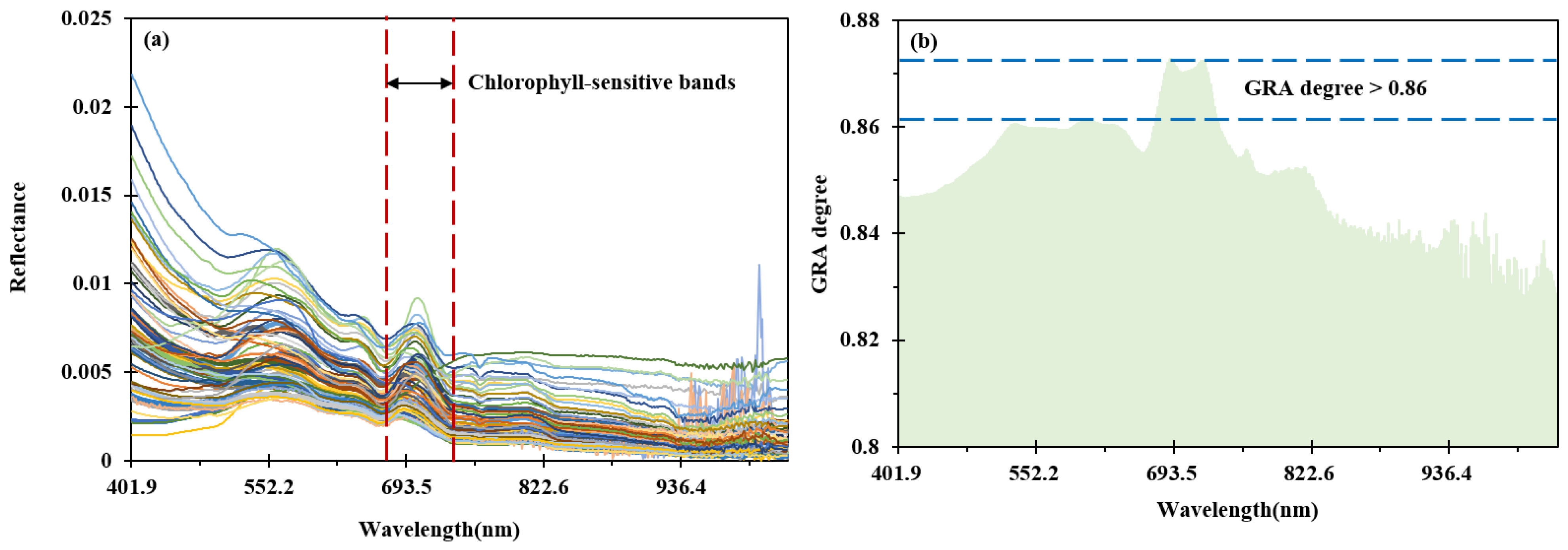
3.3. Feature Band Selection

The water spectral data were acquired in the range of 400~1000 nm, which is generally used in water color remote sensing. Figure 4a shows the 62 water reflectance spectra collected in Lake Baiyangdian. The reflectance spectra exhibit obvious chlorophyll-dominated characteristics. The absorption characteristics close to 440 and 675 nm are caused by chlorophyll absorption, and the absorption characteristic close to 620 nm is caused by phycocyanin. The absorption characteristic close to 440 nm is significantly affected by the suspended matter and CDOM, while the absorption characteristic close to 675 nm is less affected by the other water elements. Lake Baiyangdian’s water spectra exhibit a clear reflection peak close to 700 nm, which is one of the most important spectral bands of chlorophyll concentration in inland water.

Figure 4b shows the results of GRA between the spectral reflectance and the TP concentration. The GRA degree of all of the bands is >0.8, and the band with a higher GRA degree is close to 700 nm, consistent with the chlorophyll-sensitive bands. We selected the 37 characteristic bands from 674.4~736.3 nm to predict the TP concentration. These bands include the most important spectral characteristic chlorophyll bands, including the absorption valley at 675 nm and reflection peak at 700 nm. The GRA degrees of these bands are all >0.86, and their reflectance values were used as the model input to predict TP concentration.

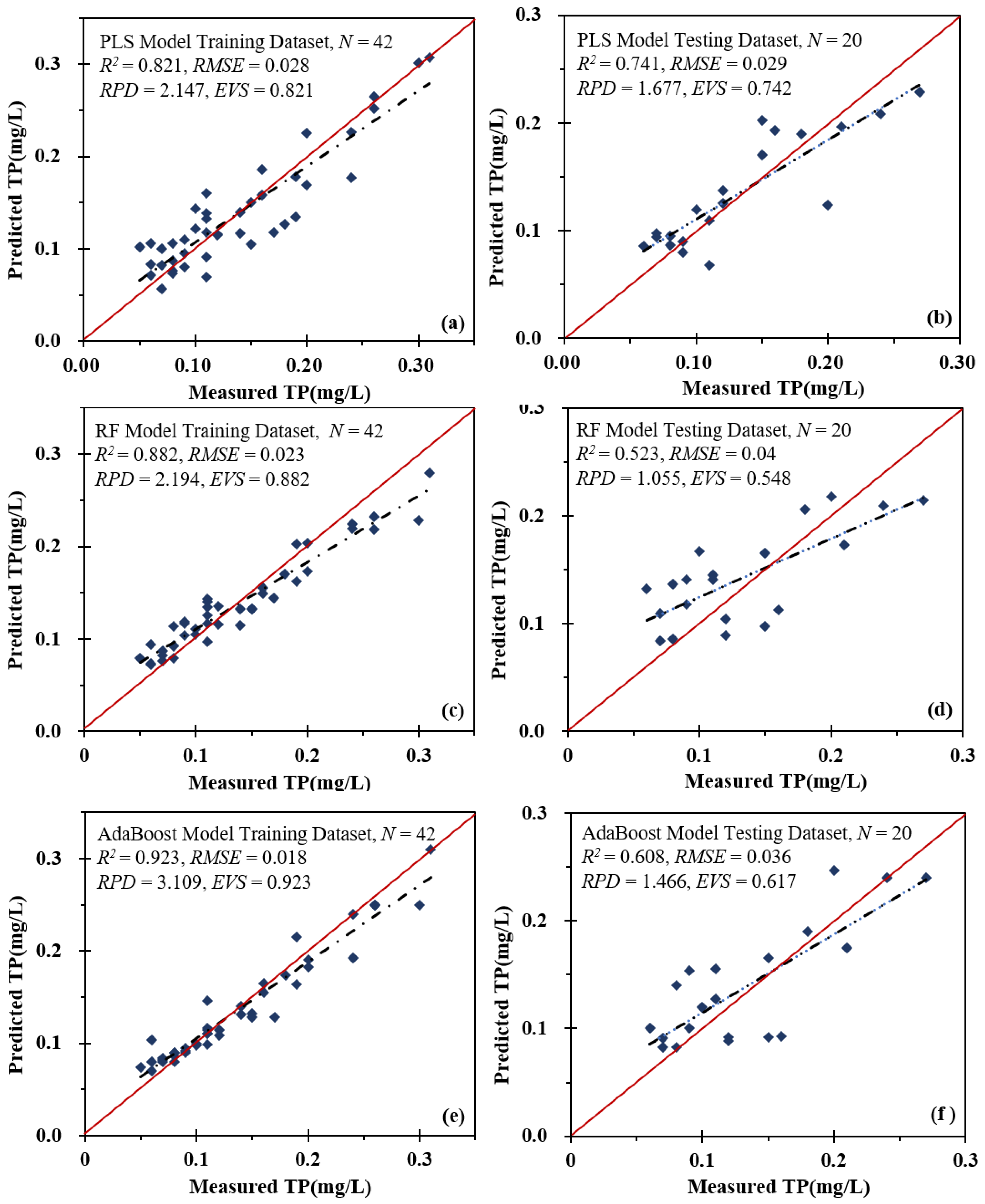
3.4. Prediction of TP Concentration

A total of 37 chlorophyll-associated spectral bands were used to predict Lake Baiyangdian’s TP concentration, with all the visible-near infrared (VNIR) bands used for comparison. To verify the chlorophyll-sensitive bands’ applicability to the TP concentration inversion, three different ML algorithms (PLS, RF, and AdaBoost) were used to construct the prediction model.

Figure 5 reveals the TP concentration prediction performance of the different ML models, using chlorophyll-sensitive bands. The R² is >0.8 in the training dataset and >0.5 in the testing dataset for all ML models. The PLS model performs well for both of the training and testing datasets, and the R² values for the training and testing datasets are 0.821 and 0.741, respectively. The R² value of the RF model in the training dataset is 0.882, but only 0.523 in the testing dataset. The RF model’s scatter plots in the testing dataset are discrete, indicating that the testing dataset’s TP concentration could not be accurately predicted. The AdaBoost model shows the best performance for the training dataset (R² = 0.923). However, its R² value is only 0.608 for the testing dataset, possibly due to overfitting. Although the PLS model accuracy is not the highest for the training dataset, it exhibits the highest accuracy for the testing dataset. Compared with the other two ML models, the R² of the PLS model is >0.7 for both the training and testing datasets, demonstrating that the PLS model performs well in terms of the TP concentration prediction.

Figure 6 further illustrates the TP concentration prediction performance of the different models using all VNIR bands. The R² values for the training dataset were 0.817, 0.877, and 0.962 for the PLS, RF, and AdaBoost models, respectively. The R² values for the testing dataset were 0.585, 0.508, and 0.596, respectively. Compared with the models established using the chlorophyll-sensitive bands, the prediction accuracy of the PLS and RF models established using all VNIR bands was lower, while the AdaBoost model’s prediction accuracy was higher for the training dataset. For the testing dataset, the accuracy of the three ML models established using all VNIR bands was lower than that of those established using the chlorophyll-sensitive bands. Although the accuracy of the AdaBoost model established using all VNIR bands was higher for the training dataset than that using the chlorophyll-sensitive bands, it performed poorly with the testing dataset, possibly as a result of overfitting in the training dataset. The verification results of the three different ML models demonstrate the feasibility of inverting the TP concentration, using chlorophyll-sensitive bands.

4. Discussion

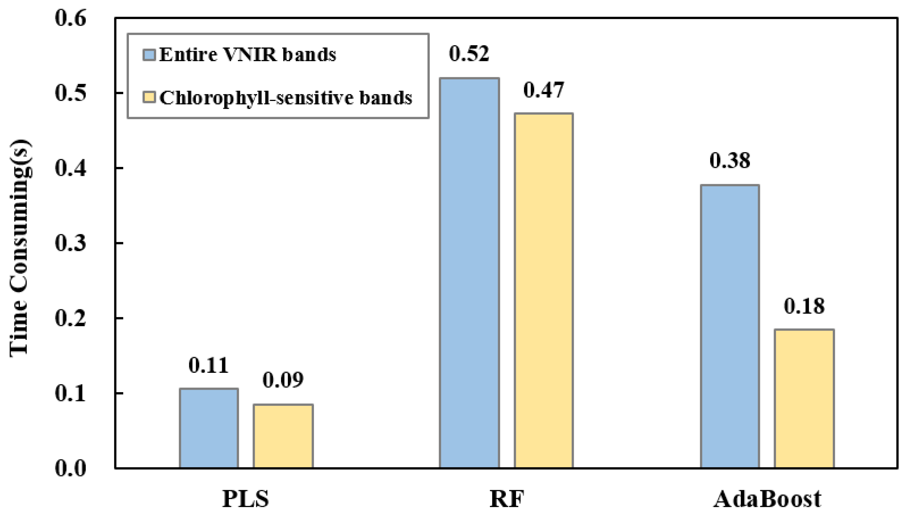
4.1. Analysis of Time Efficiency

Figure 7 illustrates the running times of different ML models predicting TP using all VNIR spectra and chlorophyll-sensitive bands. Compared with all VNIR bands, the running time for predicting TP using the chlorophyll-sensitive bands is lower, indicating that selection of the chlorophyll-sensitive bands could reduce the running time while maintaining prediction accuracy. The PLS method shows the shortest running time among the three ML models, at <0.2 s in both the chlorophyll-sensitive and VNIR bands. The RF model has the longest running time, of >0.5 s for both the chlorophyll-sensitive and VNIR bands. The RF algorithm creates a decision tree for each sample, and then obtains the prediction results for each decision tree. The final prediction result was then selected according to the vote results, which consumes a lot of time [26]. The AdaBoost model is weighted and iterated in the training process, and the weight is adjusted according to the error; thus, it also consumes more time [26,28,68]. The time difference of the AdaBoost model between the entire VNIR and chlorophyll-sensitive bands is the greatest between the three models.

Although the AdaBoost method shows the highest accuracy in the training datasets, its time consumption is also high. By contrast, the PLS method shows high accuracy and minimal time consumption. In practical application, when substantial amounts of data must be obtained in real time, the PLS models may be used to predict the TP concentration more accurately and quickly.

4.2. Effectiveness Analysis of Chlorophyll-Sensitive Bands

To verify the accuracy of the TP predictions using the chlorophyll-sensitive bands, several empirical and semi-empirical models were compared, using single band, logarithmic, ratio, difference, first- and second-order differential, and three- and four-band methods. The dataset division rules are the same as those detailed in Section 3.1. The characteristic bands selected based on the empirical and semi-empirical method and prediction accuracy are shown in

Table 3. Prediction accuracy of other models.

	Characteristic Bands (nm)	R2		RMSE
		Training Dataset	Testing Dataset	Training Dataset	Testing Dataset
Single band	713.7	0.065	0.066	0.065	0.056
Logarithmic	712.4	0.102	0.113	0.064	0.055
Ratio	703, 655	0.618	0.754	0.042	76.974
Difference	694.9, 657.8	0.662	0.701	0.039	0.035
First-order differential	675.7	0.537	0.602	0.046	0.04
Second-order differential	641	0.16	0.003	0.131	0.061
Three-band	667.5, 690.8, 745.5	0.291	0.655	0.056	0.034
Four-band	667.5, 690.8, 727, 744.2	0.002	0.006	0.067	0.058
Chlorophyll-sensitive bands	674.4~736.3	0.821	0.741	0.028	0.029

. Only the results for R² and RMSE are shown, owing to space constraints.

As Table 3 demonstrates, although the positions of the characteristic bands selected differ, depending on the empirical and semi-empirical method, they are all between 600 and 750 nm. These bands are also chlorophyll-sensitive, indicating that the chlorophyll-sensitive band reflectance has a strong correlation with TP concentration. With the exception of the ratio and difference models, which have a higher prediction accuracy (R² > 0.6), the models established using other empirical methods failed to predict the TP concentration in Lake Baiyangdian. Although the ratio model’s R² was high in both the training and testing datasets, the testing dataset’s RMSE was also high. This indicates that the ratio model could only predict the relative TP concentration accurately; the prediction error is large for the absolute value. The characteristic bands of the empirical models were selected using statistical methods, and only one or two bands were used to predict the TP concentration. The empirical models ignore the mechanisms of TP inversion and do not make full use of the rich spectral information provided by hyperspectral data, so that their applicability is low [6,8]. As a commonly used semi-empirical model, the three- and four-band methods also performed poorly in predicting the TP concentration of Lake Baiyangdian, which may be caused by an insufficient utilization of the spectral information.

In this study, we selected chlorophyll-sensitive bands ranging from 674.4 to 736.3 nm, including the strong reflection and absorption chlorophyll bands in inland water [69,70,71]. The methodology proposed herein considers the mechanism for TP inversion, and makes full use of spectral information, thus avoiding the low applicability associated with the band combinations that ignore TP inversion mechanisms. Compared with the entire VNIR model, the model established using chlorophyll-sensitive bands as input not only shows a higher accuracy for both the training and testing datasets, but also reduces the running time, which has an advantage when substantial amounts of data need to be obtained in real time.

4.3. Spatial Distribution Characteristics of Water Samples

The Environmental Quality Standards for Surface Water of China (EQSSWC; standard number: GB3838-2002) categorize the water quality into five classes, which may be used to objectively evaluate water pollution. Class I water, which is the best quality, is used for source water and national nature reserves; class V has the worst quality and is applicable to areas with agricultural and landscape requirements. In light of the ecological function of Lake Baiyangdian, its TP concentration should be in the range of 0.02~0.2 mg/L; however, the concentrations at some of the sampling points exceeded the standard. Based on the EQSSWC, the water quality of each class was determined according to the TP concentration, and the TP concentration of water samples in Lake Baiyangdian is categorized into classes II–V (Figure 1).

As Figure 1 illustrates, most of the sampling points contained class III water; class V water was the least prevalent. The sampling points containing class II water are distributed in the north and east of Lake Baiyangdian; class III water is mainly distributed in the middle of the lake; and class IV and V water are mainly distributed in the west. The sampling points with serious water pollution (containing class IV and V water) are distributed in the west of Lake Baiyangdian, close to residential areas. By contrast, the sampling points containing class II water are mainly distributed close to the large area of water bodies. The main sources of pollution in Lake Baiyangdian include tourism, agriculture, aquaculture, and domestic wastewater [37,46,49]. Copious amounts of domestic sewage are discharged into the river, leading to more severe pollution in residential areas than elsewhere [39,46]. The lake’s water quality impacts local residents’ health and plays a key role in the local ecosystem. It is thus a matter of some urgency to mitigate local domestic sewage discharge, improve water quality, and conserve the ecological environment of Lake Baiyangdian.

5. Conclusions

TP monitoring is of great significance to monitor and treat water environments. However, as an optically inactive substance, TP concentration is difficult to invert using physical models. In this paper, Lake Baiyangdian was taken as the study area, and the WT de-noising method was used to remove background noise and extract the water’s weak spectral information. Considering the correlation between TP and chlorophyll, the chlorophyll-sensitive bands were selected by GRA, and the TP concentration prediction model was constructed based on three ML algorithms (PLS, RF, and AdaBoost). The results demonstrate that the PLS model shows the best performance among the three ML algorithms in the testing dataset, with the least time consumption: the R² and RMSE are 0.741 and 0.029 mg/L, respectively. Compared with the empirical model, the method proposed herein has a higher prediction accuracy. Future studies will investigate the correlation between the chlorophyll and TP in other lakes, and verify the method proposed in this paper.

References

1. Zhang, L.; Wang, S.; Cen, Y.; Huang, C.; Zhang, H.; Sun, X.; Tong, Q. Monitoring Spatio-Temporal Dynamics in the Eastern Plain Lakes of China Using Long-Term MODIS UNWI Index. Remote Sens. 2022, 14, 985. [Google Scholar] [CrossRef]
2. Wang, S.; Zhang, L.; Zhang, H.; Han, X.; Zhang, L. Spatial–Temporal Wetland Landcover Changes of Poyang Lake Derived from Landsat and HJ-1A/B Data in the Dry Season from 1973–2019. Remote Sens. 2020, 12, 1595. [Google Scholar] [CrossRef]
3. Han, X.; Feng, L.; Hu, C.; Chen, X. Wetland changes of China’s largest freshwater lake and their linkage with the Three Gorges Dam. Remote Sens. Environ. 2018, 204, 799–811. [Google Scholar] [CrossRef]
4. Hou, X.; Feng, L.; Tang, J.; Song, X.-P.; Liu, J.; Zhang, Y.; Wang, J.; Xu, Y.; Dai, Y.; Zheng, Y.; et al. Anthropogenic transformation of Yangtze Plain freshwater lakes: Patterns, drivers and impacts. Remote Sens. Environ. 2020, 248, 111998. [Google Scholar] [CrossRef]
5. Guan, Q.; Feng, L.; Hou, X.; Schurgers, G.; Zheng, Y.; Tang, J. Eutrophication changes in fifty large lakes on the Yangtze Plain of China derived from MERIS and OLCI observations. Remote Sens. Environ. 2020, 246, 111890. [Google Scholar] [CrossRef]
6. Du, C.; Wang, Q.; Li, Y.; Lyu, H.; Zhu, L.; Zheng, Z.; Wen, S.; Liu, G.; Guo, Y. Estimation of total phosphorus concentration using a water classification method in inland water. Int. J. Appl. Earth Obs. Geoinf. 2018, 71, 29–42. [Google Scholar] [CrossRef]
7. Gao, Y.; Gao, J.; Yin, H.; Liu, C.; Xia, T.; Wang, J.; Huang, Q. Remote sensing estimation of the total phosphorus concentration in a large lake using band combinations and regional multivariate statistical modeling techniques. J. Environ. Manag. 2015, 151, 33–43. [Google Scholar] [CrossRef]
8. Sun, D.; Qiu, Z.; Li, Y.; Shi, K.; Gong, S. Detection of Total Phosphorus Concentrations of Turbid Inland Waters Using a Remote Sensing Method. Water Air Soil Pollut. 2014, 225, 1953. [Google Scholar] [CrossRef]
9. Wu, C.; Wu, J.; Qi, J.; Zhang, L.; Huang, H.; Lou, L.; Chen, Y. Empirical estimation of total phosphorus concentration in the mainstream of the Qiantang River in China using Landsat TM data. Int. J. Remote Sens. 2010, 31, 2309–2324. [Google Scholar] [CrossRef]
10. Schilling, K.E.; Kim, S.-W.; Jones, C.S. Use of water quality surrogates to estimate total phosphorus concentrations in Iowa rivers. J. Hydrol. Reg. Stud. 2017, 12, 111–121. [Google Scholar] [CrossRef]
11. Liu, C.; Zhu, L.; Li, J.; Wang, J.; Ju, J.; Qiao, B.; Ma, Q.; Wang, S. The increasing water clarity of Tibetan lakes over last 20 years according to MODIS data. Remote Sens. Environ. 2021, 253, 112199. [Google Scholar] [CrossRef]
12. Kuhn, C.; de Matos Valerio, A.; Ward, N.; Loken, L.; Sawakuchi, H.O.; Kampel, M.; Richey, J.; Stadler, P.; Crawford, J.; Striegl, R.; et al. Performance of Landsat-8 and Sentinel-2 surface reflectance products for river remote sensing retrievals of chlorophyll-a and turbidity. Remote Sens. Environ. 2019, 224, 104–118. [Google Scholar] [CrossRef] [Green Version]
13. Hu, C.; Chen, Z.; Clayton, T.D.; Swarzenski, P.; Brock, J.C.; Muller–Karger, F.E. Assessment of estuarine water-quality indicators using MODIS medium-resolution bands: Initial results from Tampa Bay, FL. Remote Sens. Environ. 2004, 93, 423–441. [Google Scholar] [CrossRef]
14. Doxaran, D.; Lamquin, N.; Park, Y.-J.; Mazeran, C.; Ryu, J.-H.; Wang, M.; Poteau, A. Retrieval of the seawater reflectance for suspended solids monitoring in the East China Sea using MODIS, MERIS and GOCI satellite data. Remote Sens. Environ. 2014, 146, 36–48. [Google Scholar] [CrossRef]
15. Domagalski, J.; Lin, C.; Luo, Y.; Kang, J.; Wang, S.; Brown, L.R.; Munn, M.D. Eutrophication study at the Panjiakou-Daheiting Reservoir system, northern Hebei Province, People’s Republic of China: Chlorophyll-a model and sources of phosphorus and nitrogen. Agric. Water Manag. 2007, 94, 43–53. [Google Scholar] [CrossRef]
16. Shi, K.; Zhang, Y.; Zhou, Y.; Liu, X.; Zhu, G.; Qin, B.; Gao, G. Long-term MODIS observations of cyanobacterial dynamics in Lake Taihu: Responses to nutrient enrichment and meteorological factors. Sci. Rep. 2017, 7, 40326. [Google Scholar] [CrossRef] [Green Version]
17. Song, K.; Li, L.; Tedesco, L.; Li, S.; Shi, K.; Hall, B. Remote Estimation of Nutrients for a Drinking Water Source Through Adaptive Modeling. Water Resour. Manag. 2014, 28, 2563–2581. [Google Scholar] [CrossRef]
18. Huang, C.; Guo, Y.; Yang, H.; Li, Y.; Zou, J.; Zhang, M.; Lyu, H.; Zhu, A.; Huang, T. Using Remote Sensing to Track Variation in Phosphorus and Its Interaction With Chlorophyll-a and Suspended Sediment. IEEE J. Sel. Top. Appl. Earth Obs. Remote Sens. 2015, 8, 4171–4180. [Google Scholar] [CrossRef]
19. Li, S.; Liu, C.; Sun, P.; Ni, T. Response of cyanobacterial bloom risk to nitrogen and phosphorus concentrations in large shallow lakes determined through geographical detector: A case study of Taihu Lake, China. Sci. Total Environ. 2022, 816, 151617. [Google Scholar] [CrossRef]
20. Liang, Z.; Soranno, P.A.; Wagner, T. The role of phosphorus and nitrogen on chlorophyll a: Evidence from hundreds of lakes. Water Res. 2020, 185, 116236. [Google Scholar] [CrossRef]
21. Søndergaard, M.; Larsen, S.E.; Jørgensen, T.B.; Jeppesen, E. Using chlorophyll a and cyanobacteria in the ecological classification of lakes. Ecol. Indic. 2011, 11, 1403–1412. [Google Scholar] [CrossRef]
22. Song, K.; Li, L.; Li, S.; Tedesco, L.; Hall, B.; Li, L. Hyperspectral Remote Sensing of Total Phosphorus (TP) in Three Central Indiana Water Supply Reservoirs. Water Air Soil Pollut. 2011, 223, 1481–1502. [Google Scholar] [CrossRef]
23. Tong, Y.; Xu, X.; Zhang, S.; Shi, L.; Zhang, X.; Wang, M.; Qi, M.; Chen, C.; Wen, Y.; Zhao, Y.; et al. Establishment of season-specific nutrient thresholds and analyses of the effects of nutrient management in eutrophic lakes through statistical machine learning. J. Hydrol. 2019, 578, 124079. [Google Scholar] [CrossRef]
24. Wang, J.; Shi, T.; Yu, D.; Teng, D.; Ge, X.; Zhang, Z.; Yang, X.; Wang, H.; Wu, G. Ensemble machine-learning-based framework for estimating total nitrogen concentration in water using drone-borne hyperspectral imagery of emergent plants: A case study in an arid oasis, NW China. Environ. Pollut. 2020, 266, 115412. [Google Scholar] [CrossRef] [PubMed]
25. Liu, C.; Zhang, F.; Ge, X.; Zhang, X.; Chan, N.W.; Qi, Y. Measurement of Total Nitrogen Concentration in Surface Water Using Hyperspectral Band Observation Method. Water 2020, 12, 1842. [Google Scholar] [CrossRef]
26. Zounemat-Kermani, M.; Batelaan, O.; Fadaee, M.; Hinkelmann, R. Ensemble machine learning paradigms in hydrology: A review. J. Hydrol. 2021, 598, 126266. [Google Scholar] [CrossRef]
27. Qun’ou, J.; Lidan, X.; Siyang, S.; Meilin, W.; Huijie, X. Retrieval model for total nitrogen concentration based on UAV hyper spectral remote sensing data and machine learning algorithms–A case study in the Miyun Reservoir, China. Ecol. Indic. 2021, 124, 107356. [Google Scholar] [CrossRef]
28. Chen, B.; Mu, X.; Chen, P.; Wang, B.; Choi, J.; Park, H.; Xu, S.; Wu, Y.; Yang, H. Machine learning-based inversion of water quality parameters in typical reach of the urban river by UAV multispectral data. Ecol. Indic. 2021, 133, 108434. [Google Scholar] [CrossRef]
29. Qiao, Z.; Sun, S.; Jiang, Q.o.; Xiao, L.; Wang, Y.; Yan, H. Retrieval of Total Phosphorus Concentration in the Surface Water of Miyun Reservoir Based on Remote Sensing Data and Machine Learning Algorithms. Remote Sens. 2021, 13, 4662. [Google Scholar] [CrossRef]
30. Wang, S.; Zhang, L.; Zhang, H.; Cen, Y.; Zhang, L.; Tong, Q. Spatiotemporal variations of total suspended sediment concentrations in the Peace-Athabasca Delta during 2000 to 2020. J. Appl. Remote Sens. 2022, 16, 014524. [Google Scholar] [CrossRef]
31. Wang, X.; Zhang, F.; Ding, J. Evaluation of water quality based on a machine learning algorithm and water quality index for the Ebinur Lake Watershed, China. Sci. Rep. 2017, 7, 12858. [Google Scholar] [CrossRef] [Green Version]
32. Zhao, Y.; Wang, S.; Zhang, F.; Shen, Q.; Li, J.; Yang, F. Remote Sensing-Based Analysis of Spatial and Temporal Water Colour Variations in Baiyangdian Lake after the Establishment of the Xiong’an New Area. Remote Sens. 2021, 13, 1729. [Google Scholar] [CrossRef]
33. Li, Z.; Sun, W.; Chen, H.; Xue, B.; Yu, J.; Tian, Z. Interannual and Seasonal Variations of Hydrological Connectivity in a Large Shallow Wetland of North China Estimated from Landsat 8 Images. Remote Sens. 2021, 13, 1214. [Google Scholar] [CrossRef]
34. Zhang, X.; Zhang, J.; Li, Z.; Wang, G.; Liu, Y.; Wang, H.; Xie, J. Optimal submerged macrophyte coverage for improving water quality in a temperate lake in China. Ecol. Eng. 2021, 162, 106177. [Google Scholar] [CrossRef]
35. Yang, W.; Yan, J.; Wang, Y.; Zhang, B.T.; Wang, H. Seasonal variation of aquatic macrophytes and its relationship with environmental factors in Baiyangdian Lake, China. Sci. Total Environ. 2020, 708, 135112. [Google Scholar] [CrossRef]
36. Wang, X.; Wang, Y.; Liu, L.; Shu, J.; Zhu, Y.; Zhou, J. Phytoplankton and eutrophication degree assessment of Baiyangdian Lake wetland, China. Sci. World J. 2013, 2013, 436965. [Google Scholar] [CrossRef]
37. Tang, C.; Yi, Y.; Yang, Z.; Zhou, Y.; Zerizghi, T.; Wang, X.; Cui, X.; Duan, P. Planktonic indicators of trophic states for a shallow lake (Baiyangdian Lake, China). Limnologica 2019, 78, 125712. [Google Scholar] [CrossRef]
38. Sun, L.; Wang, J.; Wu, Y.; Gao, T.; Liu, C. Community Structure and Function of Epiphytic Bacteria Associated With Myriophyllum spicatum in Baiyangdian Lake, China. Front. Microbiol. 2021, 12, 705509. [Google Scholar] [CrossRef]
39. Zhu, H.; Liu, X.G.; Cheng, S.P. Phytoplankton community structure and water quality assessment in an ecological restoration area of Baiyangdian Lake, China. Int. J. Environ. Sci. Technol. 2020, 18, 1529–1536. [Google Scholar] [CrossRef]
40. Zhao, Y.; Yang, Z.; Xia, X.; Wang, F. A shallow lake remediation regime with Phragmites australis: Incorporating nutrient removal and water evapotranspiration. Water Res. 2012, 46, 5635–5644. [Google Scholar] [CrossRef]
41. Zhou, L.; Sun, W.; Han, Q.; Chen, H.; Chen, H.; Jin, Y.; Tong, R.; Tian, Z. Assessment of Spatial Variation in River Water Quality of the Baiyangdian Basin (China) during Environmental Water Release Period of Upstream Reservoirs. Water 2020, 12, 688. [Google Scholar] [CrossRef] [Green Version]
42. Deng, C.; Zhang, L.; Cen, Y. Retrieval of Chemical Oxygen Demand through Modified Capsule Network Based on Hyperspectral Data. Appl. Sci. 2019, 9, 4620. [Google Scholar] [CrossRef] [Green Version]
43. Zheng, C. Strategies for Managing Environmental Flows Based On the Spatial Distribution of Water Quality: A Case Study of Baiyangdian Lake, China. J. Environ. Inform. 2011, 18, 84–90. [Google Scholar] [CrossRef]
44. Zhu, M.; Wang, S.; Kong, X.; Zheng, W.; Feng, W.; Zhang, X.; Yuan, R.; Song, X.; Sprenger, M. Interaction of Surface Water and Groundwater Influenced by Groundwater Over-Extraction, Waste Water Discharge and Water Transfer in Xiong’an New Area, China. Water 2019, 11, 539. [Google Scholar] [CrossRef] [Green Version]
45. Yan, J.; Liu, J.; Ma, M. In situ variations and relationships of water quality index with periphyton function and diversity metrics in Baiyangdian Lake of China. Ecotoxicology 2014, 23, 495–505. [Google Scholar] [CrossRef]
46. Han, Q.; Tong, R.; Sun, W.; Zhao, Y.; Yu, J.; Wang, G.; Shrestha, S.; Jin, Y. Anthropogenic influences on the water quality of the Baiyangdian Lake in North China over the last decade. Sci Total Environ. 2020, 701, 134929. [Google Scholar] [CrossRef]
47. Wang, F. Long-term Water Quality Variations and Chlorophyll a Simulation with an Emphasis on Different Hydrological Periods in Lake Baiyangdian, Northern China. J. Environ. Inform. 2012, 20, 90–102. [Google Scholar] [CrossRef]
48. Li, C.; Zheng, X.; Zhao, F.; Wang, X.; Cai, Y.; Zhang, N. Effects of Urban Non-Point Source Pollution from Baoding City on Baiyangdian Lake, China. Water 2017, 9, 249. [Google Scholar] [CrossRef]
49. Dong, L.; Yang, Z.; Liu, X. Phosphorus fractions, sorption characteristics, and its release in the sediments of Baiyangdian Lake, China. Environ. Monit. Assess. 2011, 179, 335–345. [Google Scholar] [CrossRef]
50. Zhu, J.; Wang, X.; Zhang, L.; Cheng, H.; Yang, Z. System dynamics modeling of the influence of the TN/TP concentrations in socioeconomic water on NDVI in shallow lakes. Ecol. Eng. 2015, 76, 27–35. [Google Scholar] [CrossRef]
51. Wei, L.; Huang, C.; Wang, Z.; Wang, Z.; Zhou, X.; Cao, L. Monitoring of Urban Black-Odor Water Based on Nemerow Index and Gradient Boosting Decision Tree Regression Using UAV-Borne Hyperspectral Imagery. Remote Sens. 2019, 11, 2402. [Google Scholar] [CrossRef] [Green Version]
52. Niu, C.; Tan, K.; Jia, X.; Wang, X. Deep learning based regression for optically inactive inland water quality parameter estimation using airborne hyperspectral imagery. Environ. Pollut. 2021, 286, 117534. [Google Scholar] [CrossRef]
53. Niroumand-Jadidi, M.; Bovolo, F.; Bruzzone, L. Water Quality Retrieval from PRISMA Hyperspectral Images: First Experience in a Turbid Lake and Comparison with Sentinel-2. Remote Sens. 2020, 12, 3984. [Google Scholar] [CrossRef]
54. Becker, R.H.; Sayers, M.; Dehm, D.; Shuchman, R.; Quintero, K.; Bosse, K.; Sawtell, R. Unmanned aerial system based spectroradiometer for monitoring harmful algal blooms: A new paradigm in water quality monitoring. J. Great Lakes Res. 2019, 45, 444–453. [Google Scholar] [CrossRef]
55. Zhu, P.; Liu, Y.; Li, J. Optimization and Evaluation of Widely-Used Total Suspended Matter Concentration Retrieval Methods for ZY1-02D’s AHSI Imagery. Remote Sens. 2022, 14, 683. [Google Scholar] [CrossRef]
56. Tang, J.; Tian, G.; Wang, X.; Wang, X.; Song, Q. The Methods of Water Spectra Measurement and Analysis I: Above-Water Method. J. Remote Sens. 2004, 8, 37–44. [Google Scholar]
57. Liu, J.; Ding, J.; Ge, X.; Wang, J. Evaluation of Total Nitrogen in Water via Airborne Hyperspectral Data: Potential of Fractional Order Discretization Algorithm and Discrete Wavelet Transform Analysis. Remote Sens. 2021, 13, 4643. [Google Scholar] [CrossRef]
58. Zhang, X.; Qi, W.; Cen, Y.; Lin, H.; Wang, N. Denoising vegetation spectra by combining mathematical-morphology and wavelet-transform-based filters. J. Appl. Remote Sens. 2019, 13, 4643. [Google Scholar] [CrossRef] [Green Version]
59. Wang, J.; Ding, J.; Yu, D.; Ma, X.; Zhang, Z.; Ge, X.; Teng, D.; Li, X.; Liang, J.; Lizaga, I.; et al. Capability of Sentinel-2 MSI data for monitoring and mapping of soil salinity in dry and wet seasons in the Ebinur Lake region, Xinjiang, China. Geoderma 2019, 353, 172–187. [Google Scholar] [CrossRef]
60. Jin, X.; Xu, X.; Song, X.; Li, Z.; Wang, J.; Guo, W. Estimation of Leaf Water Content in Winter Wheat Using Grey Relational Analysis–Partial Least Squares Modeling with Hyperspectral Data. Agron. J. 2013, 105, 1385–1392. [Google Scholar] [CrossRef]
61. Kuo, Y.; Yang, T.; Huang, G.-W. The use of grey relational analysis in solving multiple attribute decision-making problems. Comput. Ind. Eng. 2008, 55, 80–93. [Google Scholar] [CrossRef]
62. Sun, W.; Zhang, X.; Sun, X.; Sun, Y.; Cen, Y. Predicting nickel concentration in soil using reflectance spectroscopy associated with organic matter and clay minerals. Geoderma 2018, 327, 25–35. [Google Scholar] [CrossRef]
63. Zhang, X.; Sun, W.; Cen, Y.; Zhang, L.; Wang, N. Predicting cadmium concentration in soils using laboratory and field reflectance spectroscopy. Sci. Total Environ. 2019, 650, 321–334. [Google Scholar] [CrossRef]
64. Topp, S.N.; Pavelsky, T.M.; Jensen, D.; Simard, M.; Ross, M.R.V. Research Trends in the Use of Remote Sensing for Inland Water Quality Science: Moving Towards Multidisciplinary Applications. Water 2020, 12, 169. [Google Scholar] [CrossRef] [Green Version]
65. Peterson, K.; Sagan, V.; Sidike, P.; Cox, A.; Martinez, M. Suspended Sediment Concentration Estimation from Landsat Imagery along the Lower Missouri and Middle Mississippi Rivers Using an Extreme Learning Machine. Remote Sens. 2018, 10, 1503. [Google Scholar] [CrossRef] [Green Version]
66. Genuer, R.; Poggi, J.-M.; Tuleau-Malot, C. Variable selection using random forests. Pattern Recognit. Lett. 2010, 31, 2225–2236. [Google Scholar] [CrossRef] [Green Version]
67. Thompson, K.A.; Dickenson, E.R.V. Using machine learning classification to detect simulated increases of de facto reuse and urban stormwater surges in surface water. Water Res. 2021, 204, 117556. [Google Scholar] [CrossRef]
68. El Bilali, A.; Taleb, A.; Brouziyne, Y. Groundwater quality forecasting using machine learning algorithms for irrigation purposes. Agric. Water Manag. 2021, 245, 106625. [Google Scholar] [CrossRef]
69. Le, C.; Li, Y.; Zha, Y.; Sun, D.; Huang, C.; Lu, H. A four-band semi-analytical model for estimating chlorophyll a in highly turbid lakes: The case of Taihu Lake, China. Remote Sens. Environ. 2009, 113, 1175–1182. [Google Scholar] [CrossRef]
70. Dall’Olmo, G.; Gitelson, A.A.; Rundquist, D.C. Towards a unified approach for remote estimation of chlorophyll-a in both terrestrial vegetation and turbid productive waters. Geophys. Res. Lett. 2003, 30, 1938. [Google Scholar] [CrossRef] [Green Version]
71. Matthews, M.W. A current review of empirical procedures of remote sensing in inland and near-coastal transitional waters. Int. J. Remote Sens. 2011, 32, 6855–6899. [Google Scholar] [CrossRef]
Figure 1. (a) Baiyangdian’s location in China; (b) experimental site; and (c) water samples distribution.
Remotesensing 14 03077 g001
Figure 2. Study flowchart.
Remotesensing 14 03077 g002
Figure 3. Sketch map of wavelet decomposition.
Remotesensing 14 03077 g003
Figure 4. (a) Water spectra of Baiyangdian lake and (b) GRA results.
Remotesensing 14 03077 g004
Figure 5. Scatter plots of measured and predicted TP concentrations in Lake Baiyangdian using chlorophyll-sensitive bands (note: the red line is the 1:1 line), (a) PLS model in the training dataset; (b) PLS model in the testing dataset; (c) RF model in the training dataset; (d) RF model in the testing dataset; (e) AdaBoost model in the training dataset; (f) AdaBoost model in the testing dataset.
Remotesensing 14 03077 g005
Figure 6. Scatter plots of measured and predicted TP concentrations in Lake Baiyangdian using the entire VNIR band (note: the red line is the 1:1 line), (a) PLS model in the training dataset; (b) PLS model in the testing dataset; (c) RF model in the training dataset; (d) RF model in the testing dataset; (e) AdaBoost model in the training dataset; (f) AdaBoost model in the testing dataset.
Remotesensing 14 03077 g006
Figure 7. Running time comparison of different ML models.
Remotesensing 14 03077 g007