
Spatial and Temporal Biomass and Growth for Grain Crops Using NDVI Time Series

 ,
,  , ,
, ,
Abstract
:
1. Introduction
2. Materials and Methods
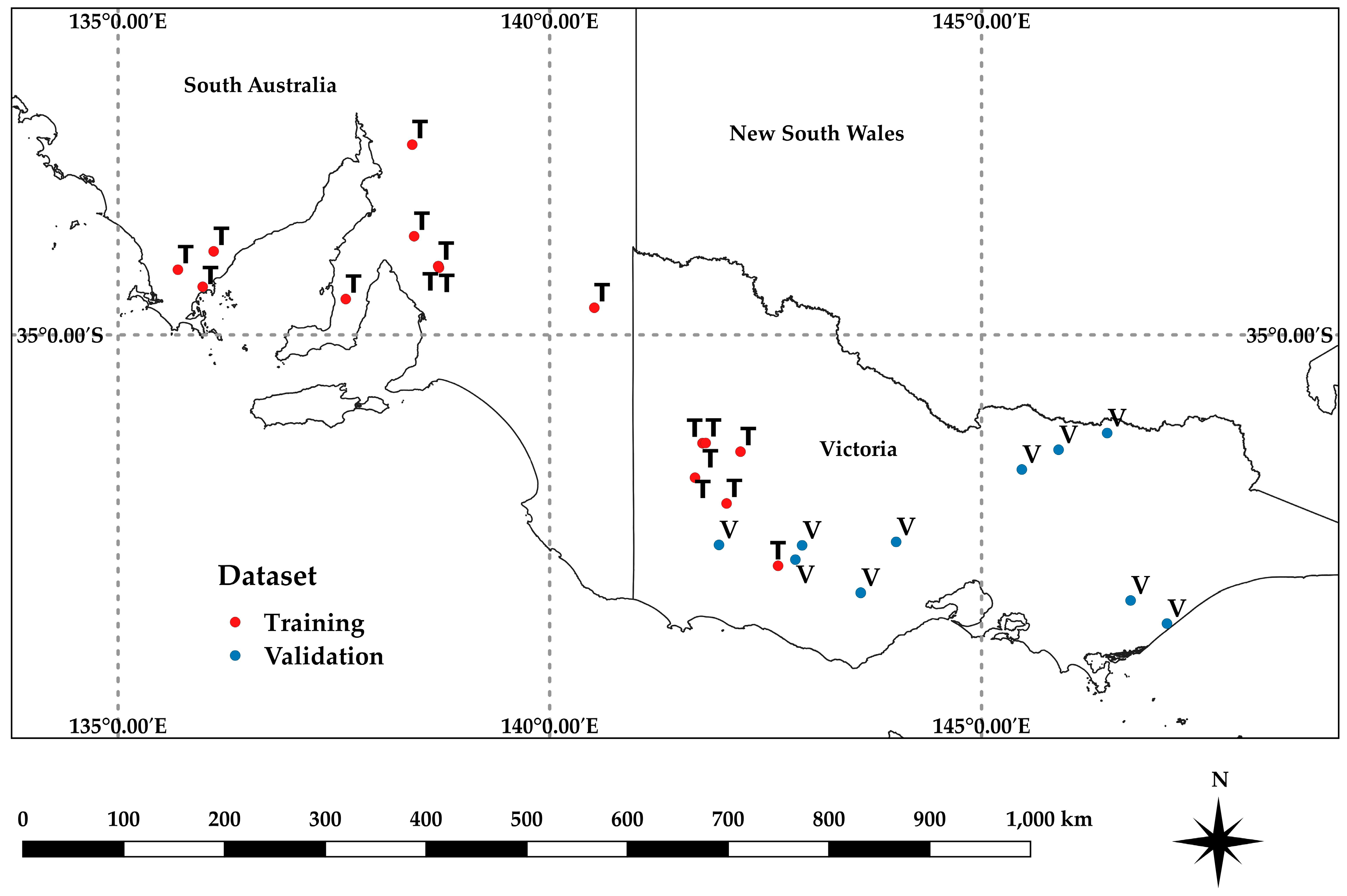
2.1. AGB Ground-Truth Datasets
2.2. Satellite Imagery Used
2.3. Ground-Based NDVI Measurements
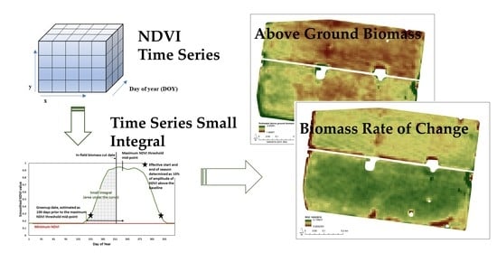
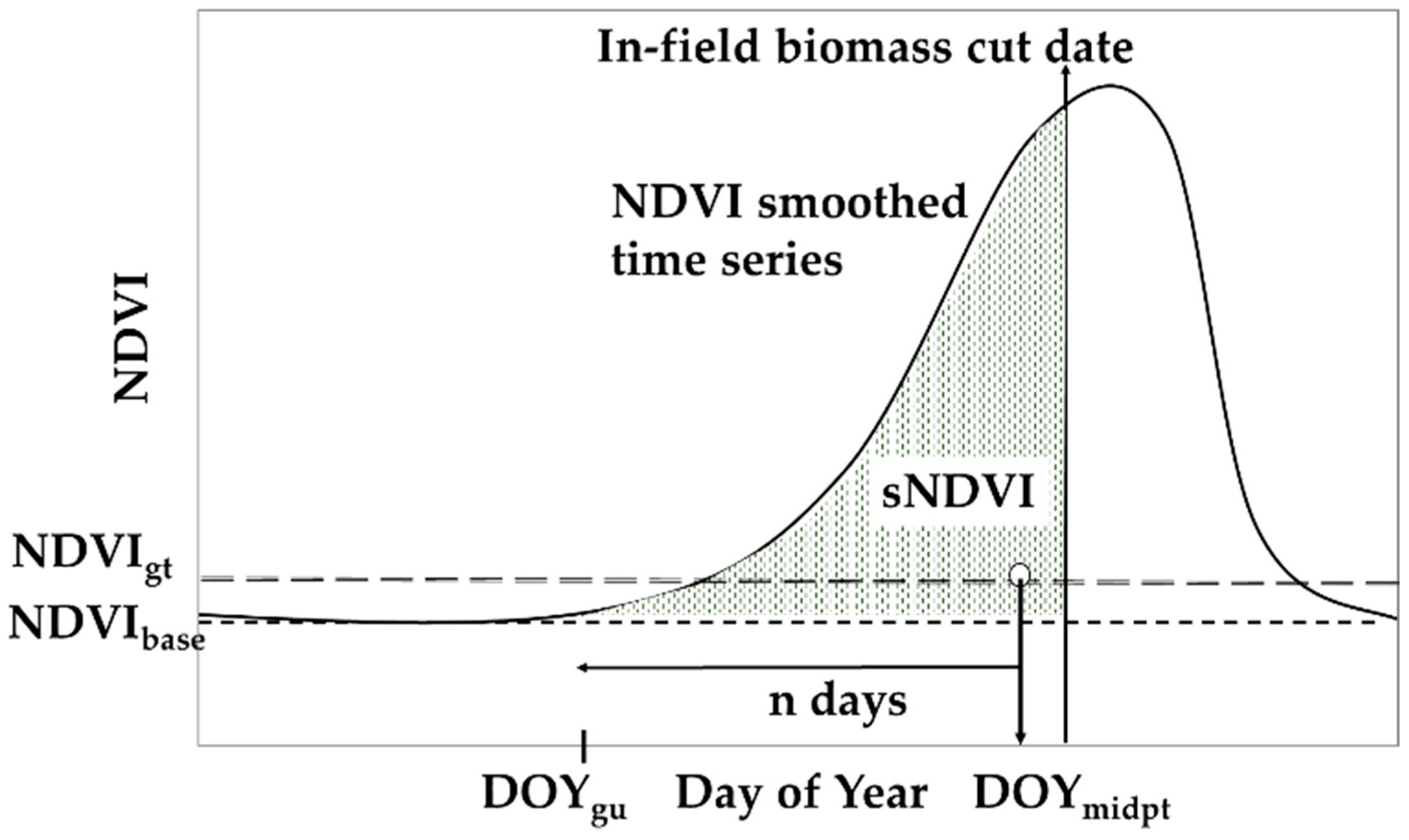
2.4. Determining the Small Integral of the NDVI Time Series
- Step 1:
- Interpolate the time series
- Step 2:
- Determine the start, end, and mid-point of the season
- Step 3:
- Calculate the small integral (summed NDVI, sNDVI)
2.5. Software Used
3. Results
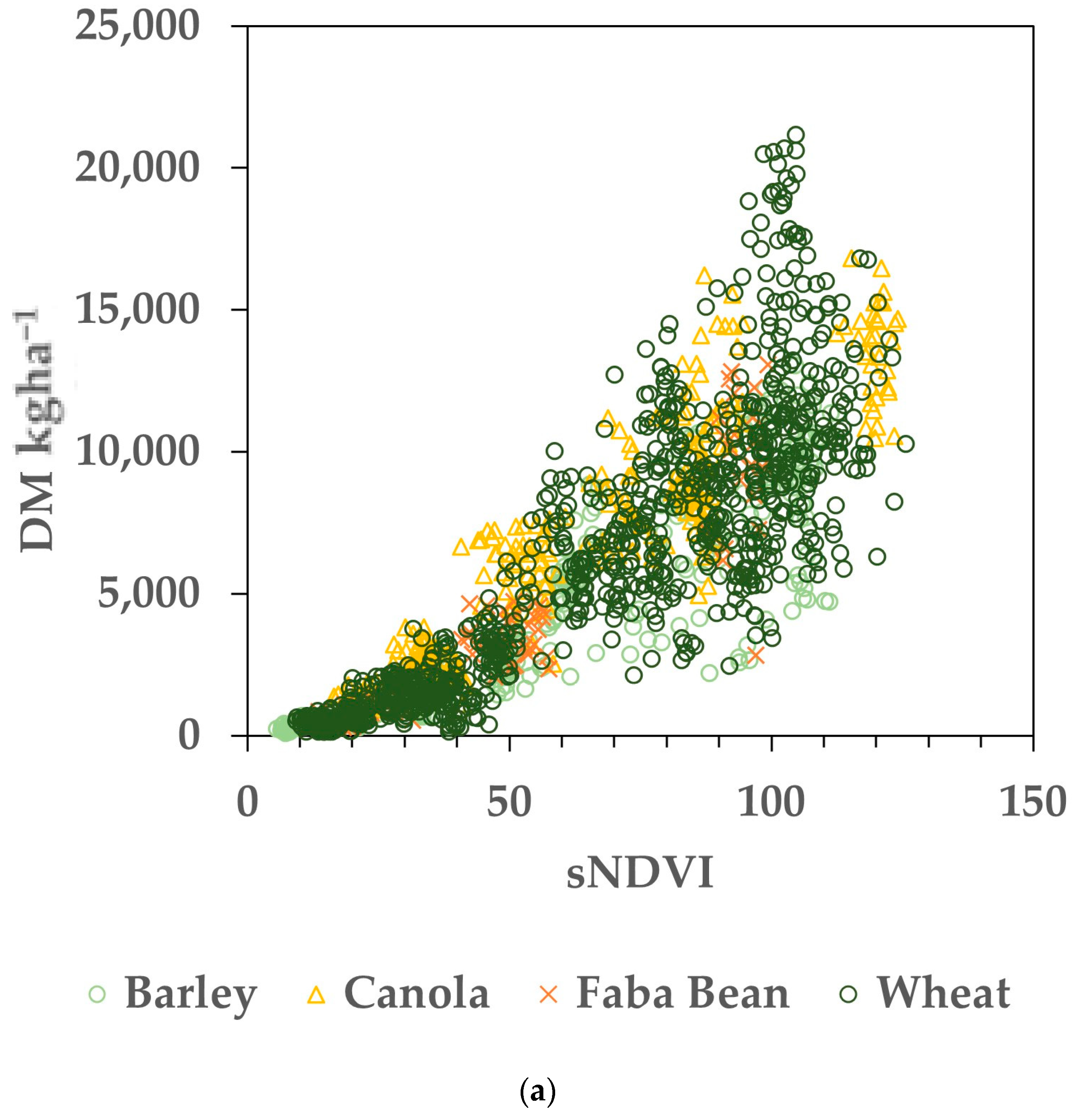
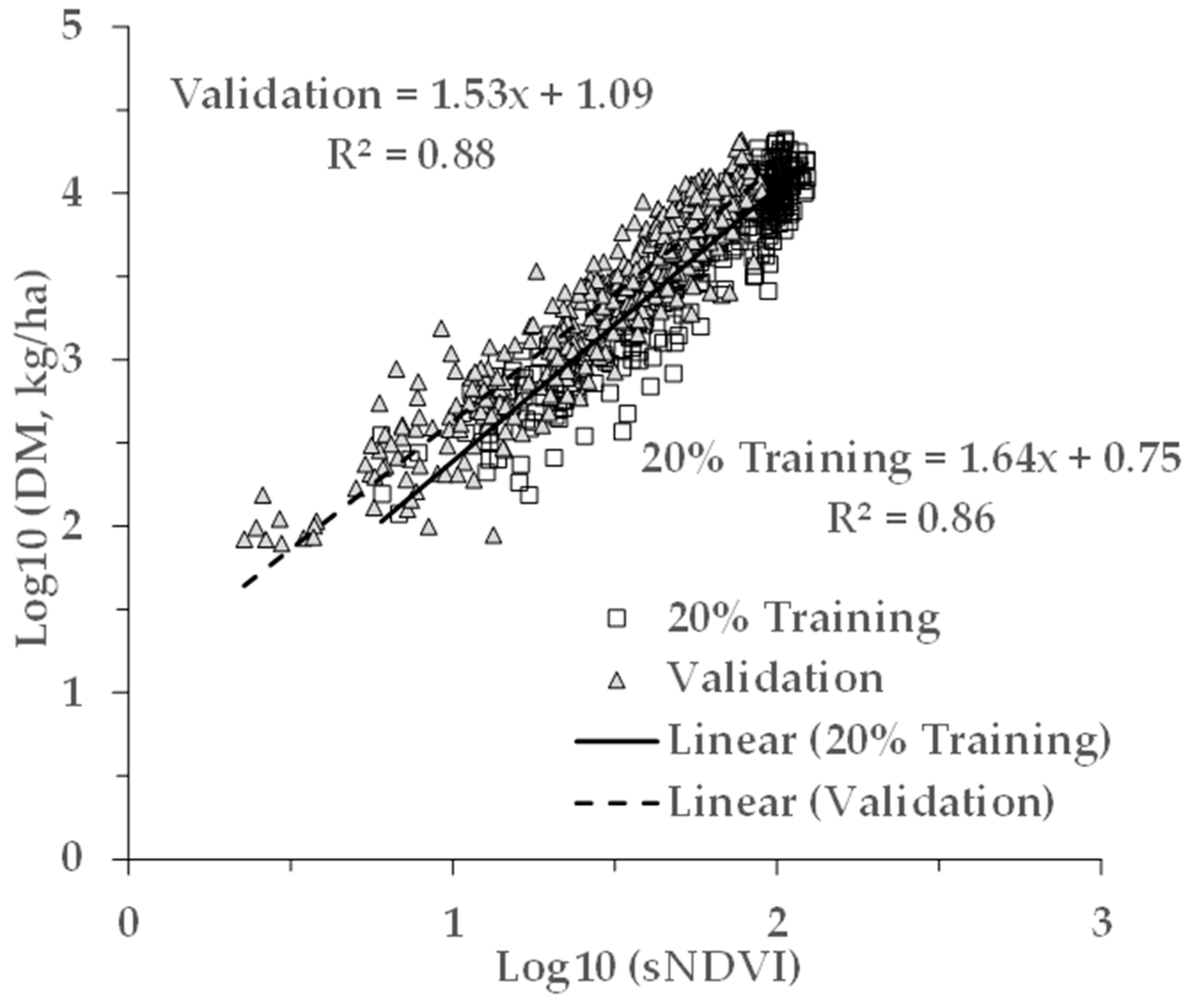
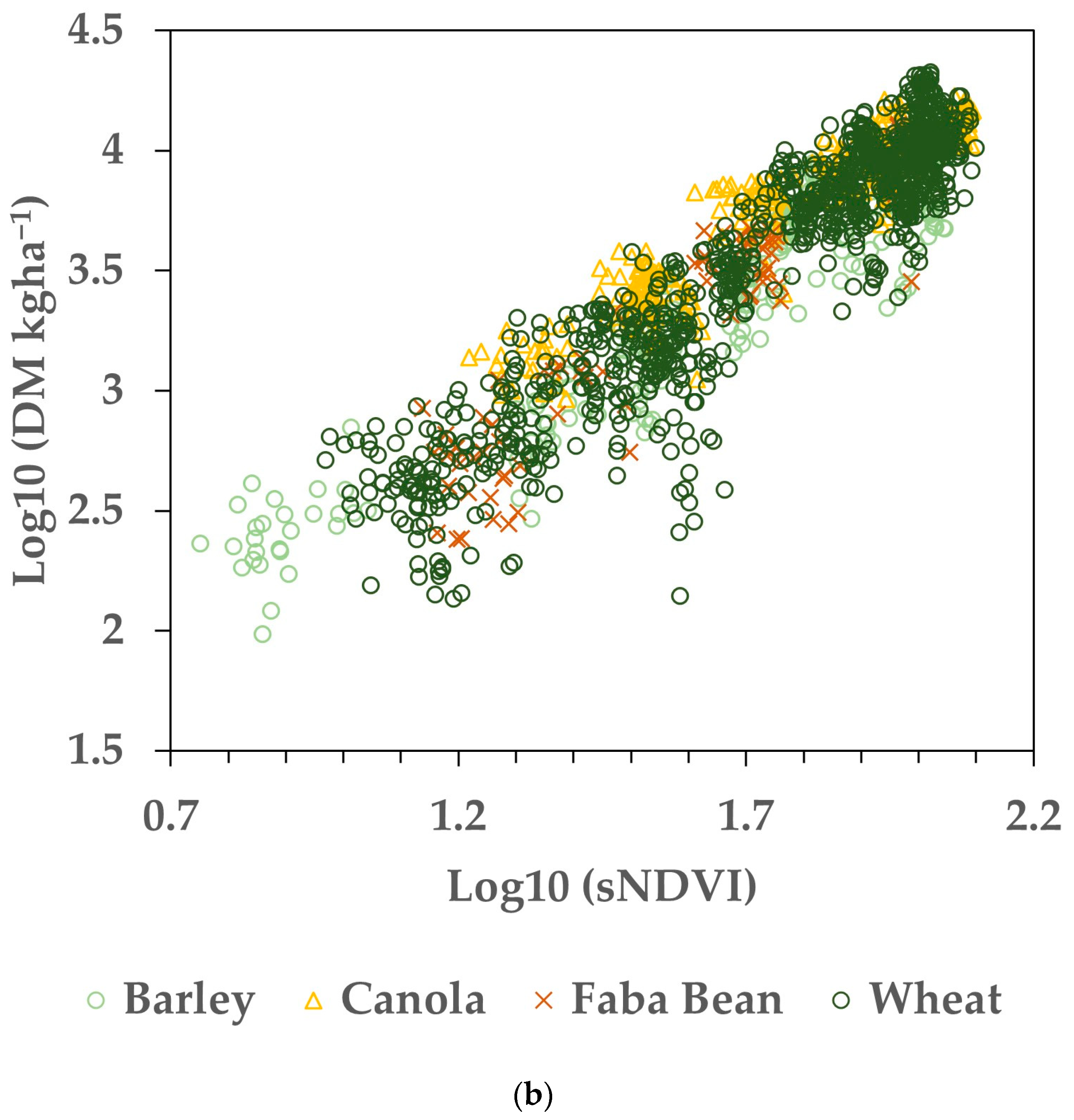
3.1. Relating Biomass to the Small Integral
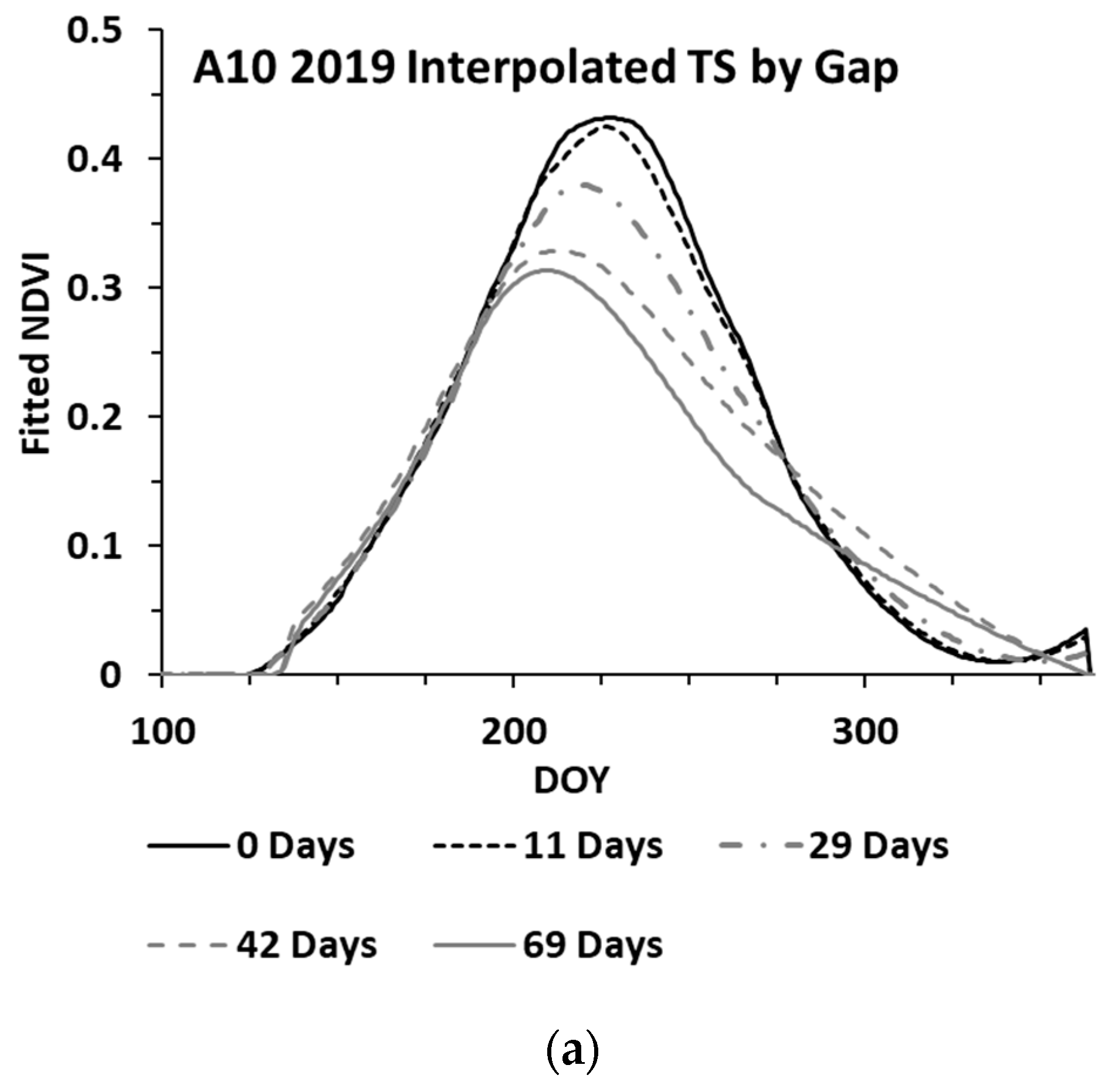
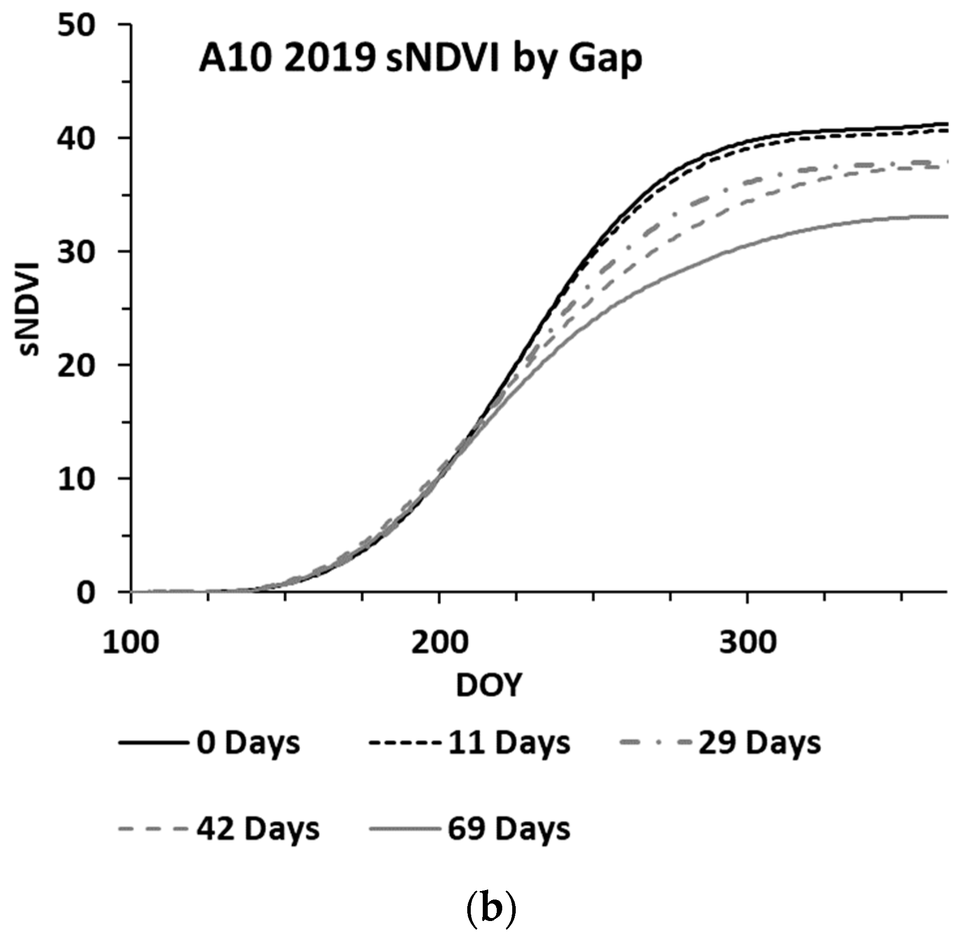
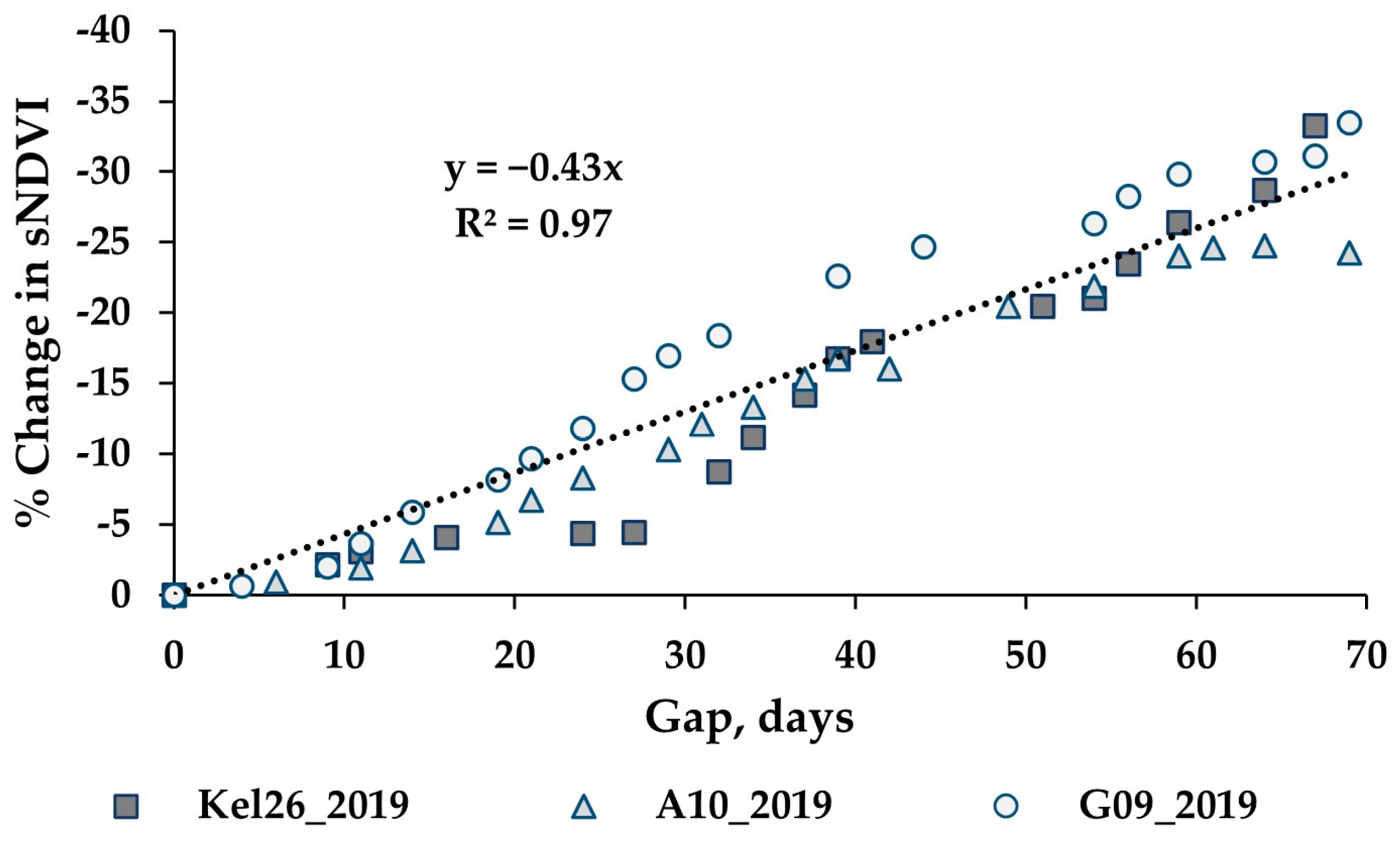
3.2. Evaluating the Effects of Gaps in the Time Series
3.3. Filling of Gaps in the Time Series
4. Discussion
5. Conclusions
Author Contributions
Funding
Data Availability Statement
Acknowledgments
Conflicts of Interest
References
- Tucker, C.J.; Holben, B.N.; Elgin, J.H.; McMurtrey, J.E. Remote sensing of total dry-matter accumulation in winter wheat. Remote Sens. Environ. 1981, 11, 171–189. [Google Scholar] [CrossRef] [Green Version]
- Asrar, G.; Kanemasu, E.T.; Jackson, R.D.; Pinter, P.J. Estimation of total above-ground phytomass production using remotely sensed data. Remote Sens. Environ. 1985, 17, 211–220. [Google Scholar] [CrossRef]
- Fu, Y.; Yang, G.; Wang, J.; Song, X.; Feng, H. Winter wheat biomass estimation based on spectral indices, band depth analysis and partial least squares regression using hyperspectral measurements. Comput. Electron. Agric. 2014, 100, 51–59. [Google Scholar] [CrossRef]
- Ghosh, P.; Mandal, D.; Bhattacharya, A.; Nanda, M.K.; Bera, S. Assessing crop monitoring potential of Sentinal-2 in a spatio-temporal scale. In Proceedings of the International Archives of the Photogrammetry, Remote Sensing and Spatial Information Sciences, Volume XLII-5, ISPRS TC V Mid-Term Symposium “Geospatial Technology-Pixel to People”, Dehradun, India, 20–23 November 2018. [Google Scholar]
- Li, C.; Li, H.; Li, J.; Lei, Y.; Li, C.; Manevski, K.; Shen, Y. Using NDVI percentiles to monitor real-time crop growth. Comput. Electron. Agric. 2019, 162, 357–363. [Google Scholar] [CrossRef]
- Battude, M.; Al Bitar, A.; Morin, D.; Cros, J.; Huc, M.; Marais Sicre, C.; Le Dantec, V.; Demarez, V. Estimating maize biomass and yield over large areas using high spatial and temporal resolution Sentinel-2 like remote sensing data. Remote Sens. Environ. 2016, 184, 668–681. [Google Scholar] [CrossRef]
- Campos, I.; González-Gómez, L.; Villodre, J.; González-Piqueras, J.; Suyker, A.E.; Calera, A. Remote sensing-based crop biomass with water or light-driven crop growth models in wheat commercial fields. Field Crop. Res. 2018, 216, 175–188. [Google Scholar] [CrossRef]
- Liao, C.; Wang, J.; Dong, T.; Shang, J.; Liu, J.; Song, Y. Using spatio-temporal fusion of Landsat-8 and MODIS data to derive phenology, biomass and yield estimates for corn and soybean. Sci. Total Environ. 2019, 650, 1707–1721. [Google Scholar] [CrossRef]
- Araya, S.; Ostendorf, B.; Lyle, G.; Lewis, M. Remote Sensing Derived Phenological Metrics to Assess the Spatio-Temporal growth Variability in Cropping Fields. Adv. Remote Sens. 2017, 6, 212–228. [Google Scholar] [CrossRef] [Green Version]
- Perry, E.M.; Morse-McNabb, E.M.; Nuttal, J.G.; O’Leary, G.J.; Clark, R. Managing Wheat From Space: Linking MODIS NDVI and Crop Models for Predicting Australian Dryland Wheat Biomass. IEEE J. Sel. Top. Appl. Earth Obs. Remote Sens. 2014, 7, 3724–3731. [Google Scholar] [CrossRef]
- Li, W.; Niu, Z.; Huang, N.; Wang, C.; Gao, S.; Wu, C. Airborne LiDAR technique for estimating biomass components of maize: A case study in Zhangye City, Northwest China. Ecol. Indic. 2015, 57, 486–496. [Google Scholar] [CrossRef]
- Periasamy, S. Significance of dual polarimetric synthetic aperture radar in biomass retrieval: An attempt on Sentinel-1. Remote Sens. Environ. 2018, 217, 537–549. [Google Scholar] [CrossRef]
- Wigneron, J.P.; Ferrazzoli, P.; Olioso, A.; Bertuzzi, P.; Chanzy, A. A Simple Approach To Monitor Crop Biomass from C-Band Radar Data. Remote Sens. Environ. 1999, 69, 179–188. [Google Scholar] [CrossRef]
- Rouse, J.W.; Haas, R.H.; Schell, J.; Deering, D. Monitoring the Vernal Advancement and Retrogradation (Green Wave Effect) of Natural Vegetation; Texas A&M University, Remote Sensing Center: College Station, TX, USA, 1973. [Google Scholar]
- Jönsson, P.; Eklundh, L. TIMESAT—A program for analyzing time-series of satellite sensor data. Comput. Geosci. 2004, 30, 833–845. [Google Scholar] [CrossRef] [Green Version]
- Araya, S.; Ostendorf, B.; Lyle, G.; Lewis, M. CropPhenology: An R package for extracting crop phenology from time series remotely sensed vegetation index imagery. Ecol. Inform. 2018, 46, 45–56. [Google Scholar] [CrossRef]
- Hill, M.J.; Donald, G.E. Estimating spatio-temporal patterns of agricultural productivity in fragmented landscapes using AVHRR NDVI time series. Remote Sens. Environ. 2003, 84, 367–384. [Google Scholar] [CrossRef]
- Nakayama, T. Impact of anthropogenic activity on eco-hydrological process in continental scales. Procedia Environ. Sci. 2012, 13, 87–94. [Google Scholar] [CrossRef] [Green Version]
- Yan, J.; Zhang, G.; Ling, H.; Han, F. Comparison of time-integrated NDVI and annual maximum NDVI for assessing grassland dynamics. Ecol. Indic. 2022, 136, 108611. [Google Scholar] [CrossRef]
- Calera, A.; González-Piqueras, J.; Melia, J. Monitoring barley and corn growth from remote sensing data at field scale. Int. J. Remote Sens. 2004, 25, 97–109. [Google Scholar] [CrossRef]
- Mirasi, A.; Mahmoudi, A.; Navid, H.; Valizadeh Kamran, K.; Asoodar, M.A. Evaluation of sum-NDVI values to estimate wheat grain yields using multi-temporal Landsat OLI data. Geocarto Int. 2021, 36, 1309–1324. [Google Scholar] [CrossRef]
- Tefera, A.T.; Banerjee, B.P.; Pandey, B.R.; James, L.; Puri, R.R.; Cooray, O.; Marsh, J.; Richards, M.; Kant, S.; Fitzgerald, G.J.; et al. Estimating early season growth and biomass of field pea for selection of divergent ideotypes using proximal sensing. Field Crop. Res. 2022, 277, 108407. [Google Scholar] [CrossRef]
- Julien, Y.; Sobrino, J.A. Comparison of cloud-reconstruction methods for time series of composite NDVI data. Remote Sens. Environ. 2010, 114, 618–625. [Google Scholar] [CrossRef]
- Julien, Y.; Sobrino, J.A. Optimizing and comparing gap-filling techniques using simulated NDVI time series from remotely sensed global data. Int. J. Appl. Earth Obs. Geoinf. 2019, 76, 93–111. [Google Scholar] [CrossRef]
- Kandasamy, S.; Baret, F.; Verger, A.; Neveux, P.; Weiss, M. A comparison of methods for smoothing and gap filling time series of remote sensing observations–application to MODIS LAI products. Biogeosciences 2013, 10, 4055–4071. [Google Scholar] [CrossRef] [Green Version]
- Rovira, A. Dryland mediterranean farming systems in Australia. Aust. J. Exp. Agric. 1992, 32, 801–809. [Google Scholar] [CrossRef]
- European Space Agency. Copernicus Sentinel-2 (Processed by ESA); MSI Level-2A BOA Reflectance Product; Collection 0; European Space Agency: Paris, France, 2021. [Google Scholar] [CrossRef]
- Planet Team. Planet Application Program Interface: In Space for Life on Earth; Planet Team: San Francisco, CA, USA, 2017. [Google Scholar]
- Sentinel-2 MSI Technical Guide Level-2A Algorithm Overview. Available online: https://sentinels.copernicus.eu/web/sentinel/technical-guides/sentinel-2-msi/level-2a/algorithm (accessed on 27 April 2022).
- UDM 2. Available online: https://developers.planet.com/docs/data/udm-2/ (accessed on 27 April 2022).
- Gorelick, N.; Hancher, M.; Dixon, M.; Ilyushchenko, S.; Thau, D.; Moore, R. Google Earth Engine: Planetary-scale geospatial analysis for everyone. Remote Sens. Environ. 2017, 202, 18–27. [Google Scholar] [CrossRef]
- R Core Team. R: A Language and Environment for Statistical Computing; R Foundation for Statistical Computing: Vienna, Austria, 2021. [Google Scholar]
- QGIS.org. QGIS Geographic Information System. QGIS Association. 2022. Available online: http://www.qgis.org (accessed on 20 June 2022).
- Ratcliff, C.; Gobbett, D.; Bramley, R. PAT-Precision Agriculture Tools; Software Collection; CSIRO: Canberra, Australia, 2019.
- Monteith, J.L. Solar Radiation and Productivity in Tropical Ecosystems. J. Appl. Ecol. 1972, 9, 747–766. [Google Scholar] [CrossRef] [Green Version]
- Meng, J.; Du, X.; Wu, B. Generation of high spatial and temporal resolution NDVI and its application in crop biomass estimation. Int. J. Digit. Earth 2013, 6, 203–218. [Google Scholar] [CrossRef]
- Collis, C. 3D mapping profiles soil-based constraints. In GRDC Groundcover; Grains Research Development Corporation: Canberra, Australia, 2022. [Google Scholar]


| Dataset | Year | Location | State | Crop | N |
|---|---|---|---|---|---|
| Training | 2018 | Woorak | Victoria | Wheat | 162 |
| 2018 | Tarlee | Victoria | Wheat | 42 | |
| 2019 | Woorak | Victoria | Barley | 243 | |
| 2019 | Wharminda | South Australia | Wheat | 32 | |
| 2019 | Booleroo Centre | South Australia | Barley | 24 | |
| 2019 | Cummins | South Australia | Wheat | 20 | |
| 2019 | Nurcoung | Victoria | Canola | 120 | |
| 2019 | Nurrabiel | Victoria | Wheat | 120 | |
| 2019 | Blyth | South Australia | Wheat | 20 | |
| 2019 | Loxton | South Australia | Wheat | 24 | |
| 2019 | Tumby Bay | South Australia | Barley | 18 | |
| 2019 | Tarlee | South Australia | Wheat | 42 | |
| 2019 | Urania | South Australia | Wheat | 30 | |
| 2019 | Wallup | Victoria | Wheat | 120 | |
| 2019 | Wickliffe | Victoria | Wheat | 160 | |
| 2020 | Woorak | Victoria | Wheat | 158 | |
| 2020 | Nurcoung | Victoria | Wheat | 90 | |
| 2020 | Tarlee | South Australia | Barley | 42 | |
| 2020 | Wickliffe | Victoria | Canola | 120 | |
| 2021 | Nurcoung | Victoria | Faba beans | 114 | |
| 2021 | Nurrabiel | Victoria | Canola | 114 | |
| 2021 | Wallup | Victoria | Wheat | 120 | |
| 2021 | Wickliffe | Victoria | Wheat | 156 | |
| All | 2091 | ||||
| Validation | 2017 | Maroona | Victoria | Canola | 50 |
| 2017 | Newlyn | Victoria | Triticale | 60 | |
| 2017 | Seaspray | Victoria | Wheat | 60 | |
| 2017 | Winnindoo | Victoria | Wheat | 60 | |
| 2018 | Devenish | Victoria | Chickpea | 40 | |
| 2018 | Gatum | Victoria | Wheat | 40 | |
| 2018 | Lilliput | Victoria | Oats | 30 | |
| 2018 | Maroona | Victoria | Wheat | 40 | |
| 2018 | Miepoll | Victoria | Wheat | 40 | |
| 2018 | Mininera | Victoria | Canola | 30 | |
| 2018 | Seaspray | Victoria | Wheat | 40 | |
| 2018 | Werneth | Victoria | Beans | 30 | |
| 2018 | Winnindoo | Victoria | Canola | 30 | |
| All | 550 |
| Calibration, Log10(DM)~Log10(sNDVI) | Validation Log10(DM)~Log10(DMest.) | |||||||||||
|---|---|---|---|---|---|---|---|---|---|---|---|---|
| Year | Paddock | Crop | N | Slope | Int. | R2 | SE | N | Slope | Int. | R2 | SE |
| 2018 | Woorak | Wheat | 130 | 1.39 | 1.26 | 0.93 | 0.10 | 32 | 0.90 | 0.36 | 0.89 | 0.11 |
| 2019 | Woorak | Barley | 194 | 1.46 | 1.03 | 0.91 | 0.16 | 49 | 0.96 | 0.17 | 0.95 | 0.11 |
| 2019 | Nurcoung | Canola | 96 | 1.61 | 0.91 | 0.81 | 0.11 | 24 | 1.02 | −0.07 | 0.71 | 0.13 |
| 2019 | Nurrabiel | Wheat | 96 | 1.73 | 0.50 | 0.90 | 0.11 | 24 | 0.97 | 0.15 | 0.84 | 0.14 |
| 2019 | Wallup | Wheat | 101 | 1.70 | 0.64 | 0.76 | 0.17 | 25 | 1.09 | −0.40 | 0.82 | 0.18 |
| 2019 | Wickliffe | Wheat | 128 | 2.40 | −0.77 | 0.79 | 0.25 | 32 | 0.86 | 0.55 | 0.88 | 0.19 |
| 2020 | Woorak | Wheat | 125 | 1.60 | 0.81 | 0.98 | 0.08 | 31 | 0.98 | 0.04 | 0.98 | 0.07 |
| 2020 | Wickliffe | Canola | 96 | 1.22 | 1.57 | 0.93 | 0.08 | 24 | 0.99 | 0.03 | 0.89 | 0.10 |
| 2021 | Nurcoung | Faba beans | 91 | 1.69 | 0.64 | 0.89 | 0.17 | 23 | 1.06 | −0.20 | 0.91 | 0.16 |
| 2021 | Nurrabiel | Canola | 91 | 1.56 | 1.07 | 0.92 | 0.11 | 23 | 1.09 | −0.33 | 0.90 | 0.12 |
| 2021 | Wallup | Wheat | 91 | 2.03 | 0.04 | 0.94 | 0.15 | 23 | 1.03 | −0.12 | 0.96 | 0.14 |
| 2021 | Wickliffe | Wheat | 125 | 2.20 | −0.17 | 0.98 | 0.10 | 31 | 0.96 | 0.17 | 0.98 | 0.08 |
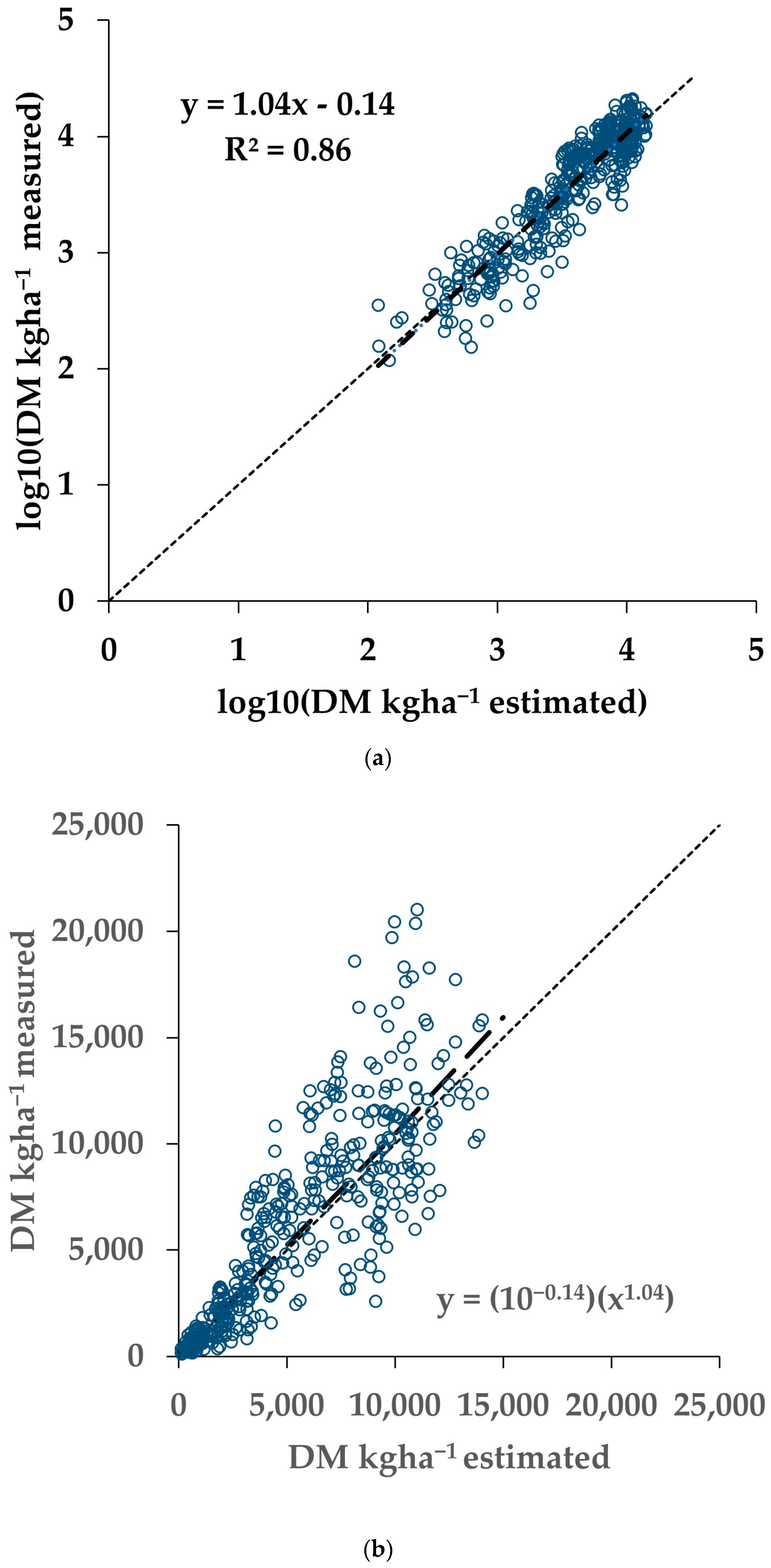
| All | All | All | 1664 | 1.57 | 0.85 | 0.86 | 0.19 | 416 | 1.04 | −0.14 | 0.86 | 0.19 |
| Paddock | DOY | AGB kg ha−1 | Gap in Imagery, Days | Change in AGB, % 1 | Gap in Imagery, Days | Change in AGB, % 1 |
|---|---|---|---|---|---|---|
| A10 2019 | 129 | 0 | 31 | 69 | ||
| 229 | 872 | 31 | −21% | 69 | −39% | |
| 310 | 3077 | 31 | −16% | 69 | −35% | |
| G09 2019 | 136 | 0 | 32 | 69 | ||
| 236 | 744 | 32 | −39% | 69 | −76% | |
| 328 | 2845 | 32 | −20% | 69 | −48% | |
| K26 2019 | 136 | 0 | 32 | 67 | ||
| 236 | 710 | 32 | −11% | 67 | −85% | |
| 330 | 2553 | 32 | −9% | 67 | −51% |
| Regression Model | N | Intercept | Slope | Adj. R2 | RMSE |
|---|---|---|---|---|---|
| Calibration: NDVIS-2~NDVIPlanet | 23,300 | −0.0512 | 1.105 | 0.95 | 0.06 |
| Validation: NDVIS-2~NDVIEstimated | 5825 | −0.0026 | 1.005 | 0.95 | 0.06 |
| Regression Model | N | Intercept | NDVIACS430 | (NDVIACS430)2 | Adj. R2 | RMSE |
|---|---|---|---|---|---|---|
| Calibration: NDVIS-2~NDVIACS430 | 1410 | −0.0308 | 2.009 | −1.05255 | 0.81 | 0.07 |
| N | Intercept | NDVIS-2 Estimated | Adj. R2 | RMSE | ||
| Validation: NDVIS-2~NDVIS-2 Estimated | 353 | 0.000 | 0.992 | 0.81 | 0.07 |
Publisher’s Note: MDPI stays neutral with regard to jurisdictional claims in published maps and institutional affiliations. |
© 2022 by the authors. Licensee MDPI, Basel, Switzerland. This article is an open access article distributed under the terms and conditions of the Creative Commons Attribution (CC BY) license (https://creativecommons.org/licenses/by/4.0/).
Share and Cite
Perry, E.; Sheffield, K.; Crawford, D.; Akpa, S.; Clancy, A.; Clark, R. Spatial and Temporal Biomass and Growth for Grain Crops Using NDVI Time Series. Remote Sens. 2022, 14, 3071. https://doi.org/10.3390/rs14133071
Perry E, Sheffield K, Crawford D, Akpa S, Clancy A, Clark R. Spatial and Temporal Biomass and Growth for Grain Crops Using NDVI Time Series. Remote Sensing. 2022; 14(13):3071. https://doi.org/10.3390/rs14133071
Chicago/Turabian StylePerry, Eileen, Kathryn Sheffield, Doug Crawford, Stephen Akpa, Alex Clancy, and Robert Clark. 2022. "Spatial and Temporal Biomass and Growth for Grain Crops Using NDVI Time Series" Remote Sensing 14, no. 13: 3071. https://doi.org/10.3390/rs14133071
APA StylePerry, E., Sheffield, K., Crawford, D., Akpa, S., Clancy, A., & Clark, R. (2022). Spatial and Temporal Biomass and Growth for Grain Crops Using NDVI Time Series. Remote Sensing, 14(13), 3071. https://doi.org/10.3390/rs14133071