A Two-Dimensional Variational Scheme for Merging Multiple Satellite Altimetry Data and Eddy Analysis

Abstract

With the increasing number of satellite altimeters in orbit, the effective resolution of merged multiple satellite altimetry data can be improved. We implement a two-dimensional variational (2-DVar) method to merge multiple satellite altimetry data and produce a daily gridded absolute dynamic topography (ADT) dataset with a grid size of 0.08 degrees. We conduct an observing system simulation experiment (OSSE), and the results show that the merged ADT dataset has an effective resolution of about 210 km. Compared with an independent sea surface temperature (SST) data, fine-scale structures can also be observed in the geostrophic flow of the new dataset. A relationship between effective resolution and the radius of a detected eddy is established and used for eddy analysis in the East China Sea (ECS) region. We observe that eddies in the open ocean are more numerous, have larger radii and live longer than those in other areas.

1. Introduction

Satellite altimeters measure sea surface height (SSH), an important variable in the study of ocean dynamics. So far, satellite altimeters provide observations only at the nadir point along the satellite ground track. For a single satellite, the distance across adjacent tracks is greater than 100 km, and the repeat time ranges from 10 to 30 days. Therefore, the spatial and temporal resolutions of the observed SSH limit its research applicability. Nevertheless, the number of altimetry satellites continues to increase, with five satellites in orbit at the time of writing. Merging measurements from multiple satellite altimeters to generate gridded datasets can help address low spatiotemporal resolution problems. In the past two decades, the Archiving, Validation, and Interpretation of Satellite Oceanographic (AVISO) has generated several multiple-satellite altimeter gridded data products that are nowadays widely used [1,2,3].

Gridded data products offer new possibilities in mesoscale eddy research [4], including eddy characterization and dynamical diagnostics. Eddy characterization refers to using gridded data products to track the movement and life cycle of mesoscale eddies [4,5,6,7,8], or to conduct statistical analyses of mesoscale eddies [8,9,10,11,12,13,14,15]. Diagnostic analysis refers to the research of eddy energy exchange and eddy viscosity estimation after mesoscale eddies are detected from the gridded data products [16,17]. In addition, gridded data products are also used in the studies of mesoscale structure and evaluation of numerical models, among other applications [18,19,20,21,22]. However, the above-mentioned applications suffer from deficiencies due to the gridded data product’s limited resolution. For example, when tracking an eddy, once the size of the eddy is smaller than the resolution threshold, it cannot be identified, resulting in eddy trajectory errors [4]. In diagnostic analyses, some quantities are very sensitive to eddy properties, such as the eddy lateral boundary viscosity, which is proportional to the size of the eddy [17]. If small eddies are excluded, such an estimate may be biased. In other applications, the gridded data products often need to be combined with other data to derive dynamic structures [23]. However, the spatial resolution mismatch between the datasets can cause problems.

The gridded data resolution mentioned above is called the effective resolution, which must be substantiated. Gridded data can be interpolated or extrapolated to any area devoid of measurements by using a merging algorithm. Still, there is a spatial scale limit that the product can resolve, which is quantified by the effective resolution. Unlike the grid step-size, an effective resolution is defined as a space–time scale of the structure that the gridded data can correctly resolve [24,25,26]. Under the current satellite altimeter data coverage, there is room for improvement of the effective resolution of nowadays merged data. We aim to improve the effective resolution of the AVISO product (hereafter referred to as AVISO). The effective resolution of AVISO is about 250–300 km in the East China Sea and its immediate regions (ECS, Figure 1a) [24]. In 2018, satellite altimeters covered almost the whole ECS (Figure 1b). The areas that are observed most are along the tracks of Jason-3 (J3, about 40 times in 2018) and Sentinel 3A (S3A, about 25 times). The areas observed least are the Bohai Sea, the Yellow Sea and the northeastern coastal area of North Korea. These areas were observed less than five times in 2018. The remaining areas of ECS were observed about five times in 2018. In this work, we implement and optimize a 2-DVar (two-dimensional variation) method to produce a gridded dataset (hereafter referred to as 2-DVar) [27]. An eddy detection method is then used to detect eddies from the 2-Dvar data.

2. Method and Data Product

A 2-DVar method is implemented to generate gridded data from along-track altimeter data [27,28].

2.1. 2-DVar Method

Absolute dynamic topography (ADT) is a variable that provides oceanic dynamic information. Unlike SSH, ADT represents the distance from the sea surface to the geoid, and not the reference ellipsoid. To be consistent with AVISO, we use the term ADT rather than SSH.

Lorenc [29] presented an optimal interpolation (OI) formulation based on the Bayesian theory. The 2-DVar method essentially uses the same algorithm as OI, but 2-DVar is computationally more flexible and suitable to solve problems that include a large amount of data. To obtain the optimal solution of a gridded ADT field, we can numerically minimize a cost function (Equation (1)):

$$J\left(\mathit{T}\right)=\frac{1}{2}{\left(\mathit{T}-{\mathit{T}}^b\right)}^T{\mathit{B}}^{-1}\left(\mathit{T}-{\mathit{T}}^b\right)+\frac{1}{2}{\sum }_{s=1}^N{\left({\mathit{H}}_s\mathit{T}-{\mathit{T}}_s^o\right)}^T{\mathit{R}}_s^{-1}\left({\mathit{H}}_s\mathit{T}-{\mathit{T}}_s^o\right)$$

(1)

where $\mathit{T}$ is an $n$-dimensional vector that encompasses the ADTs at all the grid points ($n$ is the total number of grid points), and ${\mathit{T}}^b$ is the background field. ${\mathit{T}}_s^o$ represents observations, and $N$ is the number of ADT observation types from different altimeters, where $s$ represents the corresponding sth altimeter. $\mathit{B}$ is the background error covariance matrix associated with ${\mathit{T}}^b$. ${\mathit{R}}_s$ is the observational error covariance of the observation ${\mathit{T}}_s^o$. ${\mathit{H}}_s$ is an observational operator to convert $\mathit{T}$ in the merging data grid to observation locations of ${\mathit{T}}_s^o$. In 2-DVar, the concept of increment is introduced to transform the cost function. A Cholesky decomposition technique is used to avoid calculating the inverse of $\mathit{B}$, which is essential to make it suitable for solving large data problems [28].

AVISO also uses an OI method. Thus, AVISO and 2-DVar are based on the same mathematical principle, but the background field and the associated background error covariance matrices $\mathit{B}$ are dealt with differently, leading to a difference in the effective resolution. The background error covariance matrix can be decomposed into the root-mean-square error (RMSE) diagonal matrix multiplied by the correlation coefficient matrix. That is,$\mathit{B}=\Sigma \mathit{C}\Sigma$, where $\Sigma$ is the RMSE diagonal matrix of the background error, and $\mathit{C}$ is the correlation matrix of the background error.

We note that $\mathit{C}$ is different for different background fields. In its latest DT2018 product (0.25-degree and daily sampling), AVISO uses 25 years of reanalyzed mean sea surface (MSS) as the background field [3]. Its background error is simply the sea level anomaly (SLA). The background field used in 2-DVar is the ADT field of the previous day. The background error ${\epsilon }_{2DVA\mathit{R}}$ can thus be written as ${\mathit{\epsilon }}_{\mathit{2}\mathit{D}\mathit{V}\mathit{A}\mathit{R}}=\mathit{A}\mathit{D}{\mathit{T}}_{\mathit{t}}-\mathit{A}\mathit{D}{\mathit{T}}_{\mathit{t}-\mathbf{1}}$, where $AD{T}_t$ is the ADT field of day $t$.

The background error correlation and its associated length scale of the AVISO and 2-DVar background fields are calculated and shown in Figure 2. The AVISO background error correlation coefficient is still greater than 0.6 for two points 100 km apart, which is one correlation length scale. The 2-DVar background error correlation coefficient is less than 0.6 for two points 50 km apart. This is because the AVISO background error associated with the 25-year mean is SLA, which includes large-scale signals, such as seasonal cycles and large-scale eddies, thus leading to a large correlation length scale. In 2-DVar, the background error is the ADT difference between two consecutive days. Since large-scale signals experience a limited change in such a short time, it is equivalent to filtering out most large-scale signals so that only small-scale signals remain. Therefore, the background error correlation quickly decays with distance and thus produces a smaller correlation length scale.

When constructing the correlation coefficient matrix $\mathit{C}$, a function fitting method is used to estimate the correlation length scale. The fitting function that AVISO adopts is based on Arhan and Colin de Verdière [30]. Its background error notably maintains a large correlation. Therefore, AVISO imposes excessive smoothing on the gridded data. The 2-DVar method uses a Gaussian fitting method $C=e^{-r^2/2L^2}$, where $r$ is the distance between two locations and $L$ is the correlation length scale. The resulting fitting relationship, L = 71 km, is shown in Figure 2. The smoothing effect is smaller than that of AVISO so that the gridded data can have a higher effective resolution [28].

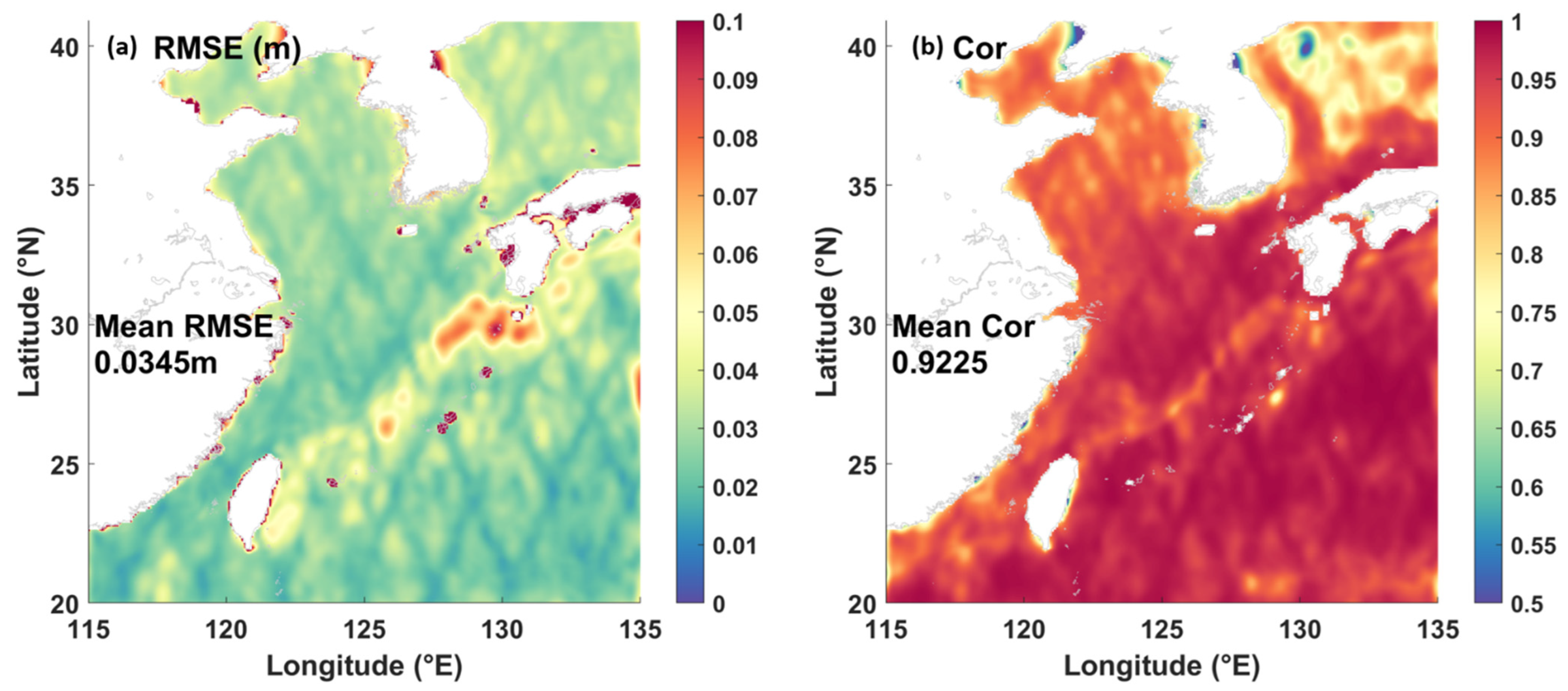
2.2. 2-DVar Gridded Data and General Evaluation

The 2-DVar method is applied to the ECS, which encompasses the area from 115 to 135°E and 20 to 45°N (Figure 1a). The mapping is performed daily for the whole of 2018 on a 0.08-degree resolution grid. The background error covariance matrix $\mathit{B}$ is constructed as described above. The RMSE of the background error is specified as 0.04 m. Unfiltered along-track ADT data from 5 satellite altimeters are used, including Cryosat-2 (C2), S3A, J3, Saral/AltiKa (SA) and HY-2A. In addition, degraded datasets using 4 satellite altimeter data (4-Sat, without S3A) and 3 satellite altimeter data (3-Sat, without S3A and SA) are made so that S3A can be regarded as independent data for validation.

To assess the error of the gridded data products, RMSEs are calculated from low-pass (65 km) filtered along-track S3A data. AVISO and 2-DVar are interpolated to S3A tracks and compared with the filtered along-track ADT provided with the AVISO product [2] (

Table 1. RMSE, correlation, useful resolution and effective resolution of all the datasets.

Dataset	RMSE (m)	Correlation	Useful Resolution (km)	Effective Resolution (km)
3-Sat	0.0726	0.9835	132	300
4-Sat	0.0665	0.9862	126	255
2-DVar	0.0364	0.9958	140	145
AVISO	0.0387	0.9953	210	175

). The correlation (RMSE) between the ADT from 2-DVar and the along-track data is slightly higher (lower) than that from AVISO. In the 2-DVar degraded datasets, the RMSEs are smaller than 0.0726 m and the correlations are higher than 0.9835.

Temporal and spatial continuities of 2-DVar are examined by calculating the geostrophic vorticities of the gridded data. Mesoscale (~100 km) real geostrophic vorticity evolutions should be smooth. A break in the evolution of geostrophic vorticity usually means a false signal caused by the mapping process. Three sampling sections (red lines in Figure 1) are selected for analysis and the temporal evolution of the geostrophic vorticity along these three sections is given in Figure 3. The results of AVISO and 2-DVar along Lines 1 and 3 are similar, with correlation coefficients of 0.62 and 0.60, respectively. The results of AVISO and 2-DVar along Line 2, sampled in the semi-closed basin, are different (correlation coefficient is 0.27). In addition, the large vorticity bands in 2-DVar are thinner than those from AVISO.

As discussed in the introduction, an effective resolution is a key parameter that characterizes a gridded data product. Two effective resolution definitions are presented here. One is defined following Chelton et al. [14] and can be written as Equation (2):

$$SR\left({\lambda }_s\right)=\frac{S_{map}\left({\lambda }_s\right)}{S_{obs}\left({\lambda }_s\right)}$$

(2)

where $S_{obs}\left({\lambda }_s\right)$ denotes the power spectral density (PSD) of along-track data, and $S_{map}\left({\lambda }_s\right)$ is the PSD of the ADT map interpolated onto the same along-track segments as those for the calculation of $S_{obs}\left({\lambda }_s\right)$. $SR\left({\lambda }_s\right)$ is the ratio at ${\lambda }_s$, where ${\lambda }_s$ is wavelength. If $SR\left({\lambda }_s\right)$ is greater than 0.5 at wavelength ${\lambda }_s$, the signal at this scale is considered to be resolved. Another is defined following Ballarotta et al. [24], expressed as (Equation 3):

$$NSR\left({\lambda }_s\right)=\frac{S_{diff}\left({\lambda }_s\right)}{S_{obs}\left({\lambda }_s\right)}$$

(3)

where $S_{diff}\left({\lambda }_s\right)$ is the PSD of the difference $(AD{T}_{obs}-AD{T}_{map})$, $AD{T}_{obs}$ is the along-track ADT and $AD{T}_{map}$ is the ADT map interpolated onto the same along-track segments. $NSR\left({\lambda }_s\right)$ is the ratio at ${\lambda }_s$, where ${\lambda }_s$ is wavelength. If $NSR\left({\lambda }_s\right)$ is less than 0.5 at wavelength ${\lambda }_s$, the signal at this scale is considered to be resolved. To differentiate the two resolution definitions, we refer to the former as “useful resolution” since it is mainly useful for verifying the available and realistic amount of energy at a specific wavelength between two signals without considering their phase. It should be noted that $SR\left({\lambda }_s\right)$ < 0.5 or $NSR\left({\lambda }_s\right)$ > 0.5 does not mean that the signal at this scale is unresolved, but its reliability is lower.

Here, both the useful and effective resolution are calculated using S3A along-track data (Figure 4 and Table 1). Figure 4a shows that the PSDs of all datasets are very close to those of S3A at a large scale (wavelengths larger than 500 km). They increasingly differ on scales smaller than 500 km. According to the above definition, compared with the S3A along-track filtered-ADT PSD, the useful resolution of AVISO is about 210 km and the useful resolution of 2-DVar is about 140 km. However, the useful resolutions of the degraded 2-DVar data are higher (126 and 132 km for 4-Sat and 3-Sat, respectively) than the normal 2-DVar data (Figure 4c). Figure 4b shows the averaged PSD from the difference between S3A and all products. In scales larger than 200 km, the PSD of differences of degraded products are larger than those of 2-DVar and AVISO. According to the effective resolution definition, the effective resolutions of normal 2-DVar, 4-Sat, 3-Sat and AVISO are 145, 255, 300 and 175 km, respectively.

The useful resolution of the degraded products is higher than that of the normal 2-DVar mapped fields and should result from the fact that the useful resolution definition does not consider the phase of signals. When S3A is not included in the mapping, non-coherent energy is not appropriately smoothed out along the S3A track. When S3A is included in the mapping, the small-scale energy is lower than that from 3-Sat or 4-Sat cases, leading to a lower useful resolution.

The effective resolution is more suitable in this study. The effective resolution improves when more information is available (more satellite altimeter data). Considering that the S3A information is included in the normal 2-DVar dataset, its effective resolution may be overestimated. The real effective resolution of 2-DVar should be between 145 and 255 km.

2.3. Observing System Simulation Experiment

It is difficult to fully evaluate the data’s performance due to the lack of independent observational data. The observing system simulation experiment (OSSE), as used by Le Guillou et al. [31], provides another way to evaluate and demonstrate the scheme. In this study, CROCO (Coastal and Regional Ocean Community), a recently developed ocean modeling system built upon ROMS_AGRIF (Regional Ocean Modeling System, Adaptive Grid, Refinement in Fortran), is employed.

CROCO is a free surface topography-following coordinate system that solves three-dimensional primitive equations. It adopts an explicit splitting scheme in time, using a shorter time step to drive SSH changes and barotropic momentum, and a longer time step to drive temperature, salinity and baroclinic momentum.

The simulation period is 2018, with a 25-year spin-up period. The model’s horizontal resolution is 1/12°, and it is vertically divided into 32 layers, with a higher vertical resolution in the upper and bottom layers. This study implements the K-profile parameterization (KPP) [32] vertical mixing scheme. The lateral boundaries are all set to open, with the CHARACT scheme [33] applied as the barotropic open boundary condition, and the baroclinic open boundary condition adopts the ORLANSKI scheme [34,35]. The lateral boundary forcing is obtained from the Global Ocean Forecasting System (GOFS 3.1) reanalysis data of the Hybrid Coordinate Ocean Model (HYCOM) with a resolution of 0.08°. The atmospheric forcing is from the Climate Forecast System Reanalysis (CFSR) data with a resolution of 0.2°. The model topography is derived from the 15-arc-second resolution data provided by the Shuttle Radar Topography Mission (SRTM). Tidal effects are not included and wind stresses are set to zero.

The daily mean SSH field is used for along-track SSH sampling. The satellite altimeter sampling data process is simulated, and the sampling times and positions are the same as those of the 5 satellite altimeters mentioned in Section 2.2. Measurement errors are also added to the sampling SSH data. The observational errors are considered to have a Gaussian distribution, and the RMSEs are set to 0.029, 0.025, 0.021, 0.031 and 0.024 m for J3, C2, SA, HY-2A and S3A, respectively. These SSH data are then used to produce an OSSE 2-DVar dataset based on the 2-DVar method.

The RMSE of OSSE 2-DVar dataset is calculated and presented in Figure 5a. The highest RMSE (>0.08 m) occurs along the main axis of Kuroshio. The RMSEs in the locations of satellite orbits are lower than in other regions, indicating that the RMSEs of 2-DVar and AVISO in Table 1 are overestimated. The mean RMSE of the study region is 0.0345 m, which is slightly higher than those in Table 1. In the open ocean, the correlation is higher than 0.9. In the Yellow and Bohai Seas, and the Sea of Japan, the correlation is lower than 0.9. The correlations in the locations of satellite orbits are higher than in other regions, indicating that the correlations of 2-DVar and AVISO in Table 1 are underestimated. The mean correlation of the study region is 0.9225, which is slightly lower than those in Table 1.

A more accurate 2-DVar useful and effective resolution can be assessed based on OSSE. The sampling locations are marked in Figure 6a, with each sampling line containing 109 grids and covering most regions of the ECS. Figure 6b shows that the SSH PSD of OSSE 2-DVar is very close to that of CROCO on the large-scale (wavelengths larger than 300 km). They increasingly differ at scales smaller than 250 km. The useful and effective resolution of OSSE 2-DVar are about 125 and 210 km, respectively (Figure 6c). The useful resolution of OSSE 2-DVar is similar to that in Table 1. On the other hand, the effective resolution of OSSE 2-DVar is much higher than that in Table 1 (between 145 and 255 km), which is consistent with the previous hypothesis.

3. Eddy Characterization

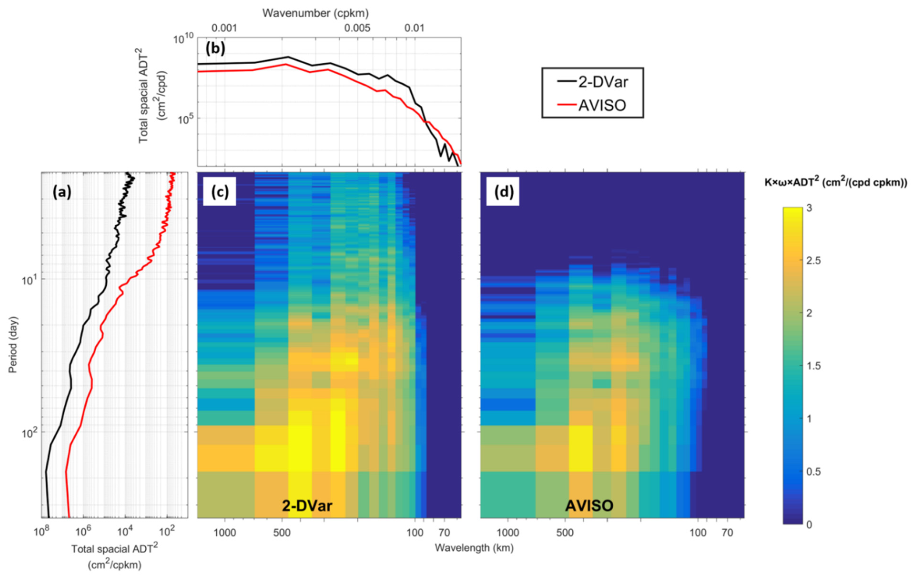
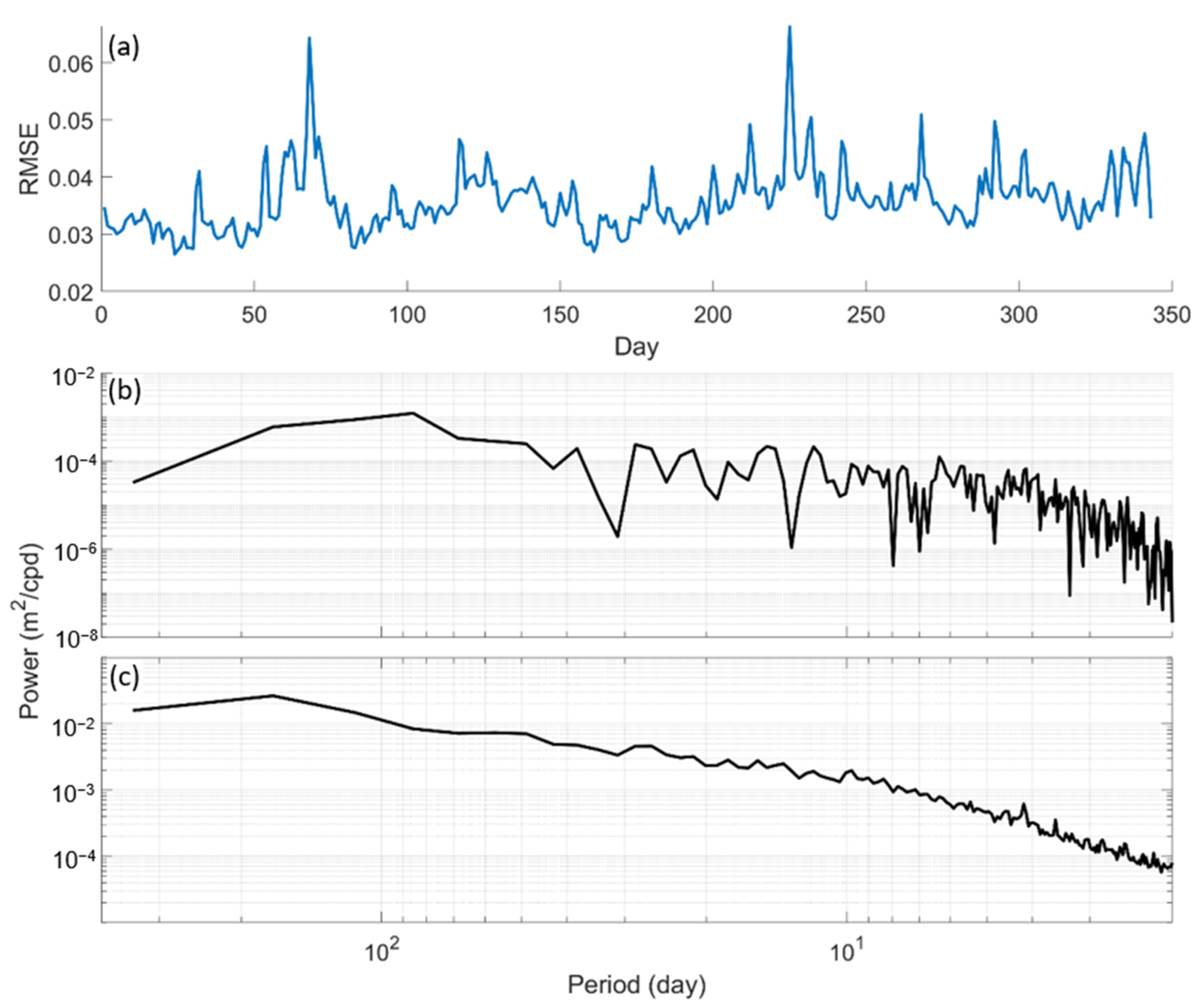
3.1. Wavenumber Frequency Spectrum Analysis

To quantify the ability of gridded datasets to resolve eddies in both temporal and spatial scales, we conducted a horizontal wavenumber frequency spectrum analysis [36,37,38] so that the temporal and spatial scale distribution of the eddy frequency power spectral density (FPSD) and PSD in the products can be jointly analyzed. The analysis area is indicated in Figure 1. Before applying the spectral analysis to the normal 2-DVar, the OSSE 2-DVar is examined to evaluate the reliable temporal and spatial scales of the signals.

Figure 7a,b shows the horizontal wavenumber frequency spectral density of SSH in the OSSE 2-DVar and CROCO field, respectively. The frequency–wavenumber power spectral density (FWPSD) of the OSSE 2-DVar is significant in the spatial scale larger than 90 km and temporal scale longer than 5 days, indicating that the OSSE 2-DVar includes energetic dynamical processes in these spatiotemporal scales. To identify the reliable spatiotemporal scales of OSSE 2-DVar, the FWPSD score (FWPSDs) is introduced, which can be defined as (Equation (4)):

$$FWPS{D}_S=1-\frac{FWPSD\left(SSH-SS{H}_{true}\right)}{FWPSD\left(SS{H}_{true}\right)}$$

(4)

where $\left(SSH-SS{H}_{true}\right)$ is the difference between the CROCO SSH $SS{H}_{true}$ and the SSH interpolated onto the CROCO grid $SSH$. This definition is similar to the NSR definition but for FWPSD. $FWPS{D}_S>0.5$ means the signal in this scale is reliable. Although OSSE 2-DVar includes energetic processes with scales of a few tens of kilometers and a couple of days, the reliable scales are larger than 160 km and longer than 23 days. Considering the result in Figure 6c, the reliable spatial scale is set to 210 km.

It is necessary to determine if the signals with smaller and shorter spatiotemporal scales (i.e., noise) are negligible in OSSE 2-DVar. A low-pass filter with a 23-day cut-off period and 210 km cut-off wavelength is applied to the CROCO and OSSE 2-DVar SSH fields and their differences. The filtered SSH is the reliable large-scale data and the residual component is the noise. The noise is ~1 order weaker than the reliable SSH (Figure 8a–f), and the differences are mainly attributed to the noises (Figure 8g–i). The analysis suggests that the reliable spatiotemporal scale is reasonable.

Based on the above results, we focus on signals with scales larger than 210 km and longer than 23 days. Figure 9c,d shows that the PSD of 2-DVar is greater than that of AVISO on time scales greater than 23 days and spatial scales greater than 210 km. This result shows that the small scale (~30 days and ~250 km) is more energetic in 2-DVar than in AVISO, suggesting that 2-DVar can resolve more small-scale eddies.

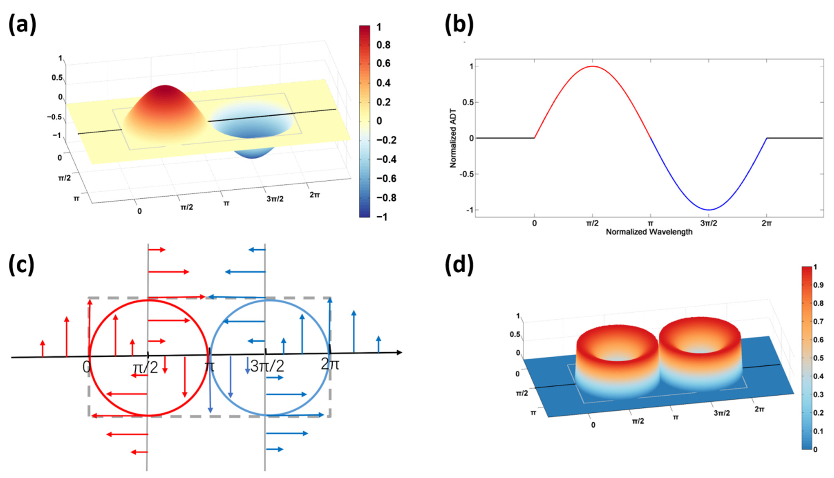
3.2. Eddy Structures

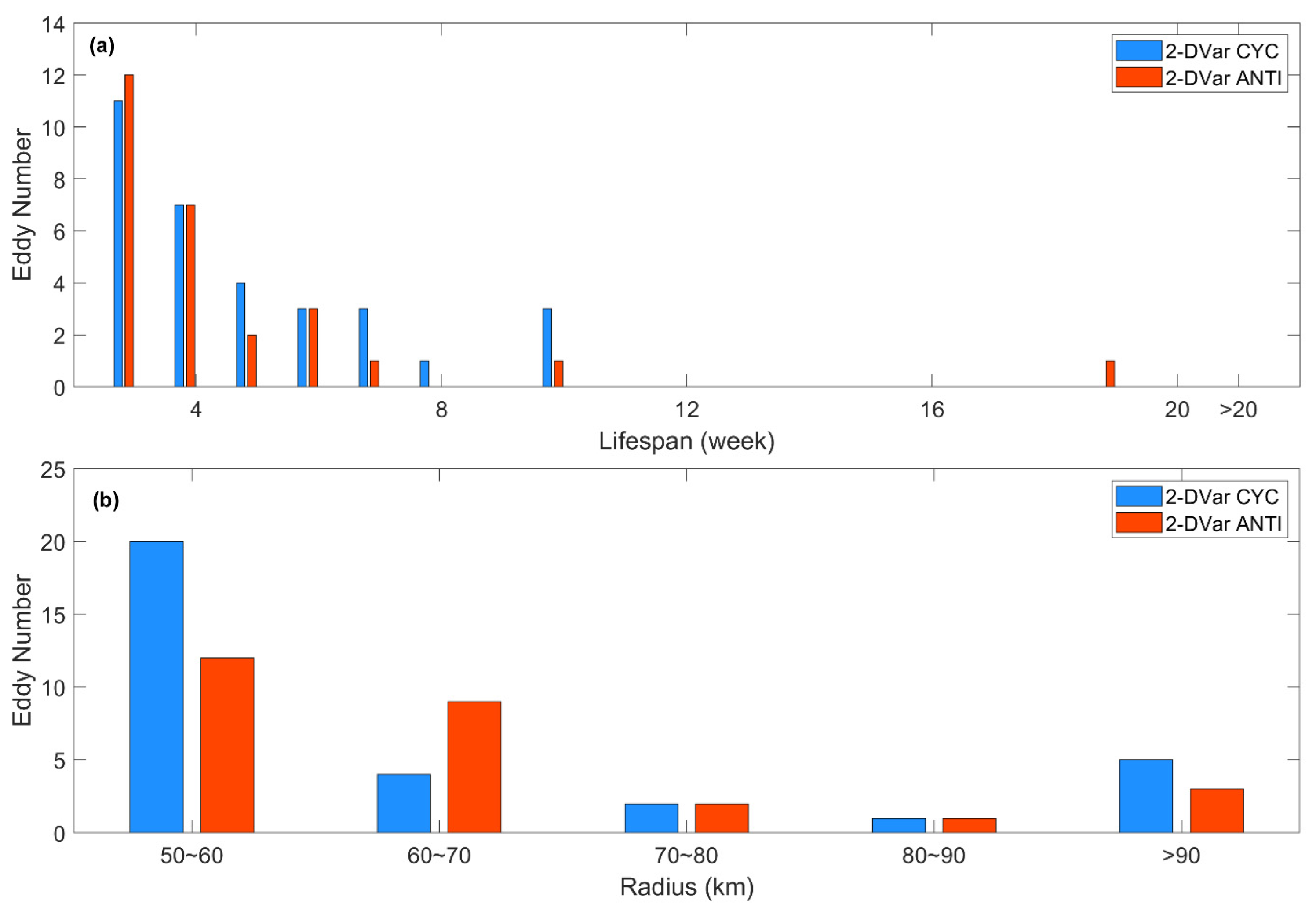
Due to the divergence (convergence) caused by the Coriolis effect, cyclonic (anticyclonic) eddies could induce local upwelling (downwelling), resulting in negative (positive) sea surface temperature (SST) anomalies. Therefore, we can use SST to independently check eddy information. The Remote Sensing Systems (RSS) infrared (IR) SST product at 4 km spatial resolution is compared with the geostrophic currents from AVISO and 2-DVar ADT. Figure 10 shows the comparison between the 2-DVar and AVISO geostrophic currents and RSS SST on 24 May 2018. The current patterns from the two datasets agree and are consistent with the large-scale SST pattern. However, the AVISO geostrophic current velocity is generally weaker than that of 2-DVar, and the current field is smoother. The 2-DVar method displays more small-scale structures that are not observed in AVISO (red boxes of Figure 10; anticyclonic eddy on the west coast of South Korea, warm tongue on the west side of Jeju Island and warm tongue in the center of the ECS), which are consistent with local SST patterns. Such consistency demonstrates that the small-scale features from 2-DVar are real physical processes in the ocean. It is also noted that some small-scale structures do not match the SST patterns (blue boxes in Figure 10), such as a cyclonic eddy north of Taiwan Island and a small eddy structure on the north side of the Kuroshio path.

3.3. Eddy Detection

To further quantify the eddy characterization, an eddy detection method proposed by Nencioli et al. [39] is used to detect eddies from AVISO and 2-DVar data. This method detects eddies based on the geometric characteristics of the current field [40,41,42]. The geostrophic velocities are calculated from the ADT of both AVISO and 2-DVar data. Eddy detection is then conducted. To adequately reduce noises in the detection results, we set lifespan and radius thresholds for the detected eddies. Eddies with a lifespan of fewer than 23 days are discarded based on the previous reliable spatiotemporal scale analysis. A relationship between the effective resolution and the minimum resolvable eddy radius is needed before the radius threshold is determined.

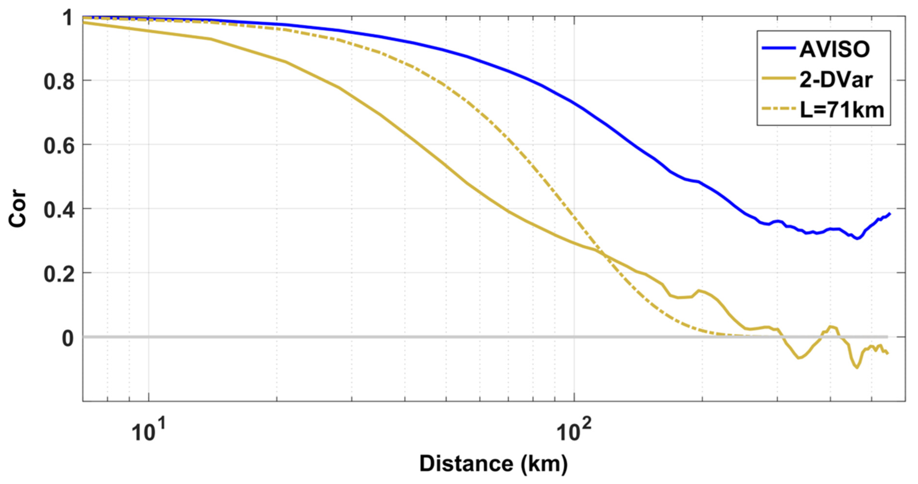
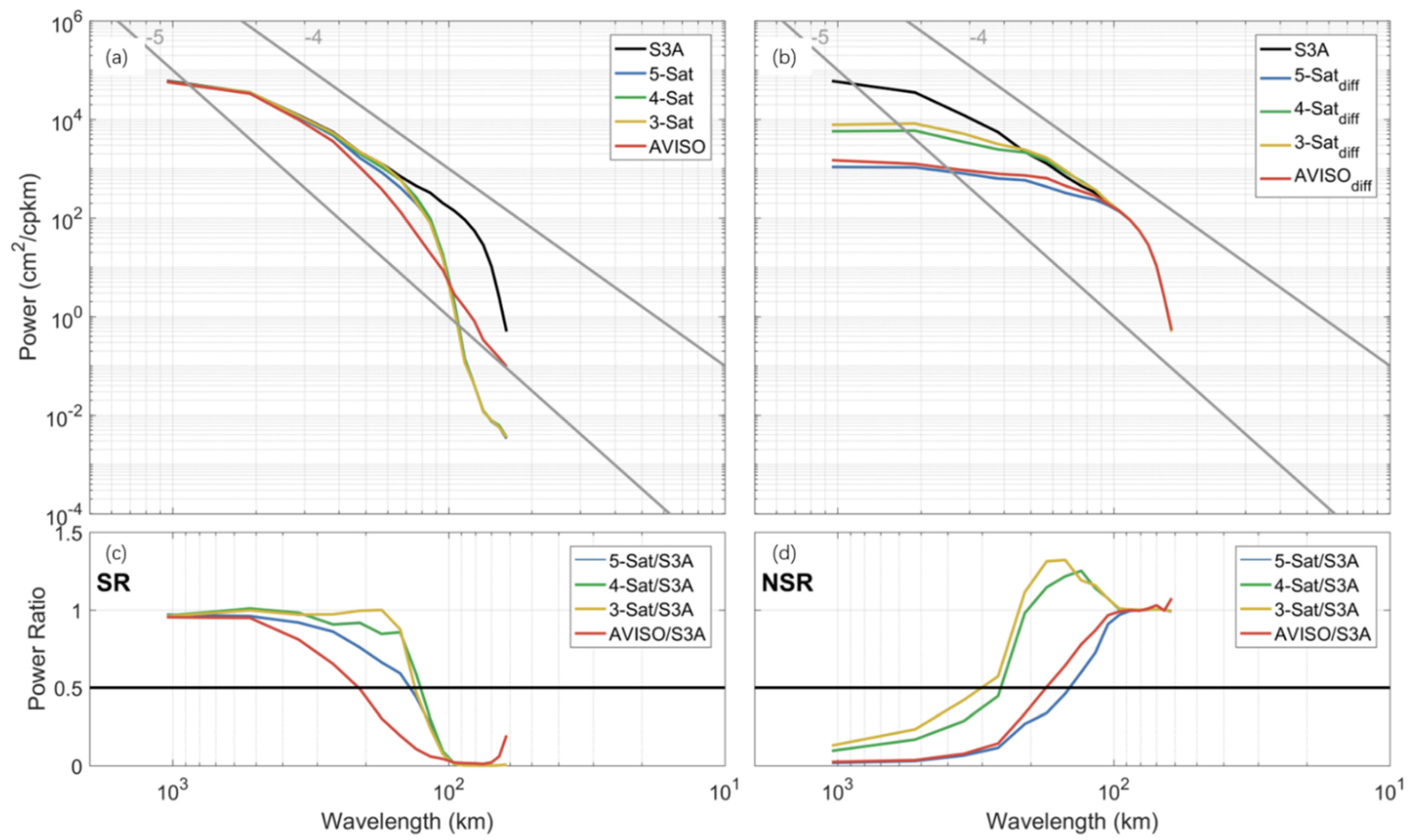
3.3.1. Effective Resolution and Eddy Size

To understand how the enhanced effective resolution is related to detected eddies, we need to determine the relationship between the effective resolution and eddy radius. To our knowledge, such a relation has not yet been established. We discuss how to establish the relationship as follows:

Equation (3) indicates that the effective resolution is based on the definition of the ADT PSD, which is defined in the wavenumber space, while the eddy radius is defined as a spatial distance. Therefore, we need to determine the relationship between the minimum resolvable eddy radius $R_{emin}$ and the wavelength ${\lambda }_x$ corresponding to the effective resolution. We assume that eddies are circular, and their edges are the location of maximum velocity. We consider an idealized case in which a pair of cyclonic and anticyclonic eddies coexist side by side (Figure 11). It shows that a sinusoidal wave contains just a pair of cyclonic and anticyclonic eddies.

The relationship between the effective resolution ${\lambda }_x$ and the minimum resolvable eddy radius $R_{emin}$ is:

$$R_{emin}=\frac{1}{4}{\lambda }_x$$

(5)

According to 2-DVar’s effective resolution shown in OSSE (210 km), the $R_{emin}$ of 2-DVar is 52.5 km. For convenience, the threshold of the eddy radius is set to 50 km.

3.3.2. Eddy Detection Evaluation

The eddy detection is examined in OSSE 2-DVar before applying it to the normal 2-DVar. One life cycle of an eddy is counted as one eddy, which includes many snapshots. Eddies with a lifespan of fewer than 23 days and a mean radius smaller than 50 km are discarded.

Table 2. Eddy number statistics of OSSE.

Mean Radius (km)	CROCO Cyclonic Eddy	2-DVar Cyclonic Eddy	CROCO Anticyclonic Eddy	2-DVar Anticyclonic Eddy
50–60	10	6	12	10
60–70	3	1	4	6
70–80	1	3	4	3
80–90	0	2	0	0
>90	10	8	1	1
Sum	24	19	21	20

shows the eddy number detected from both CROCO SSH results and OSSE 2-DVar. Compared with the detection result of CROCO, OSSE 2-DVar underestimates the total number of cyclonic and anticyclonic eddies by 20% and 4%, respectively.

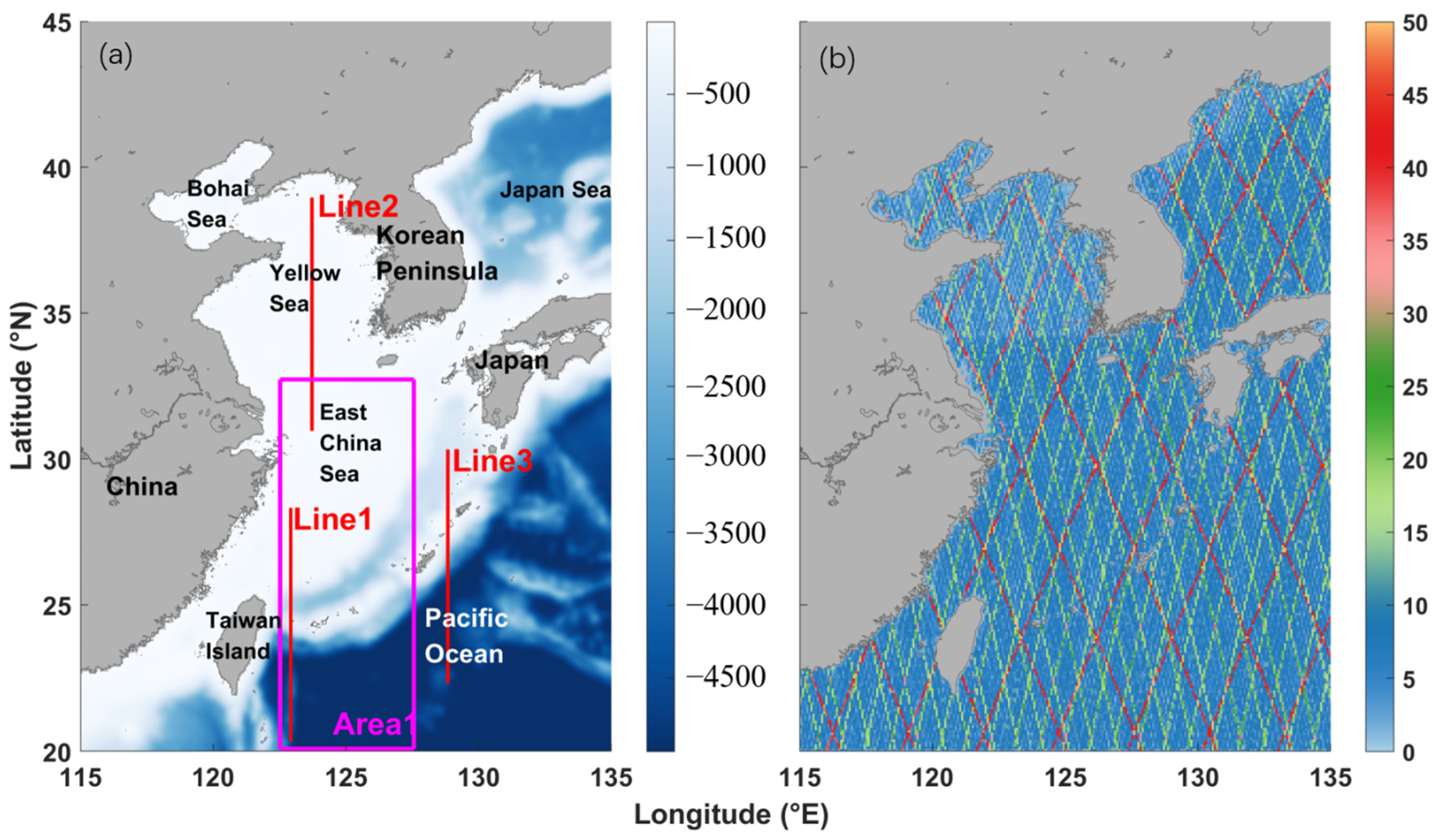
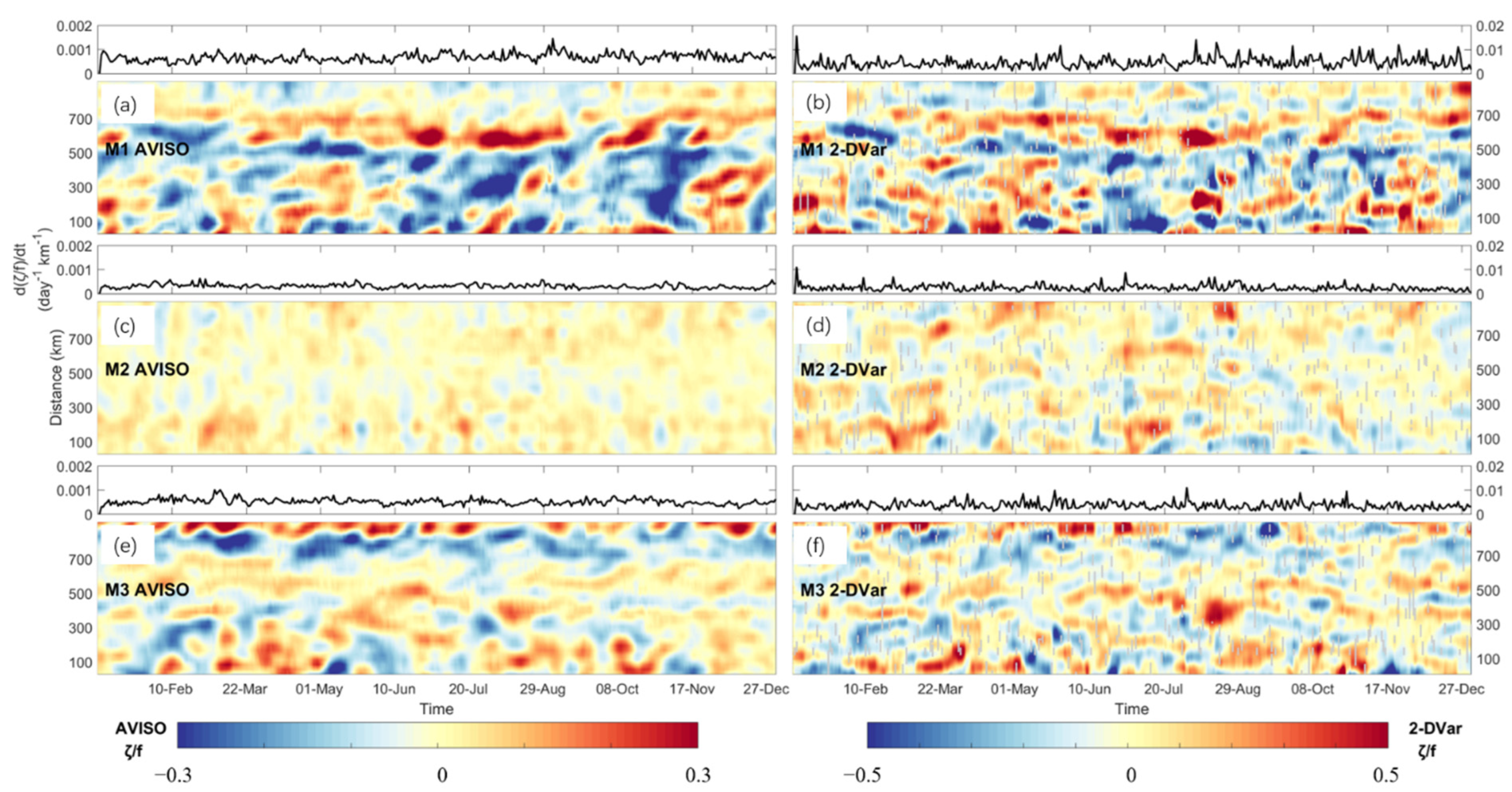
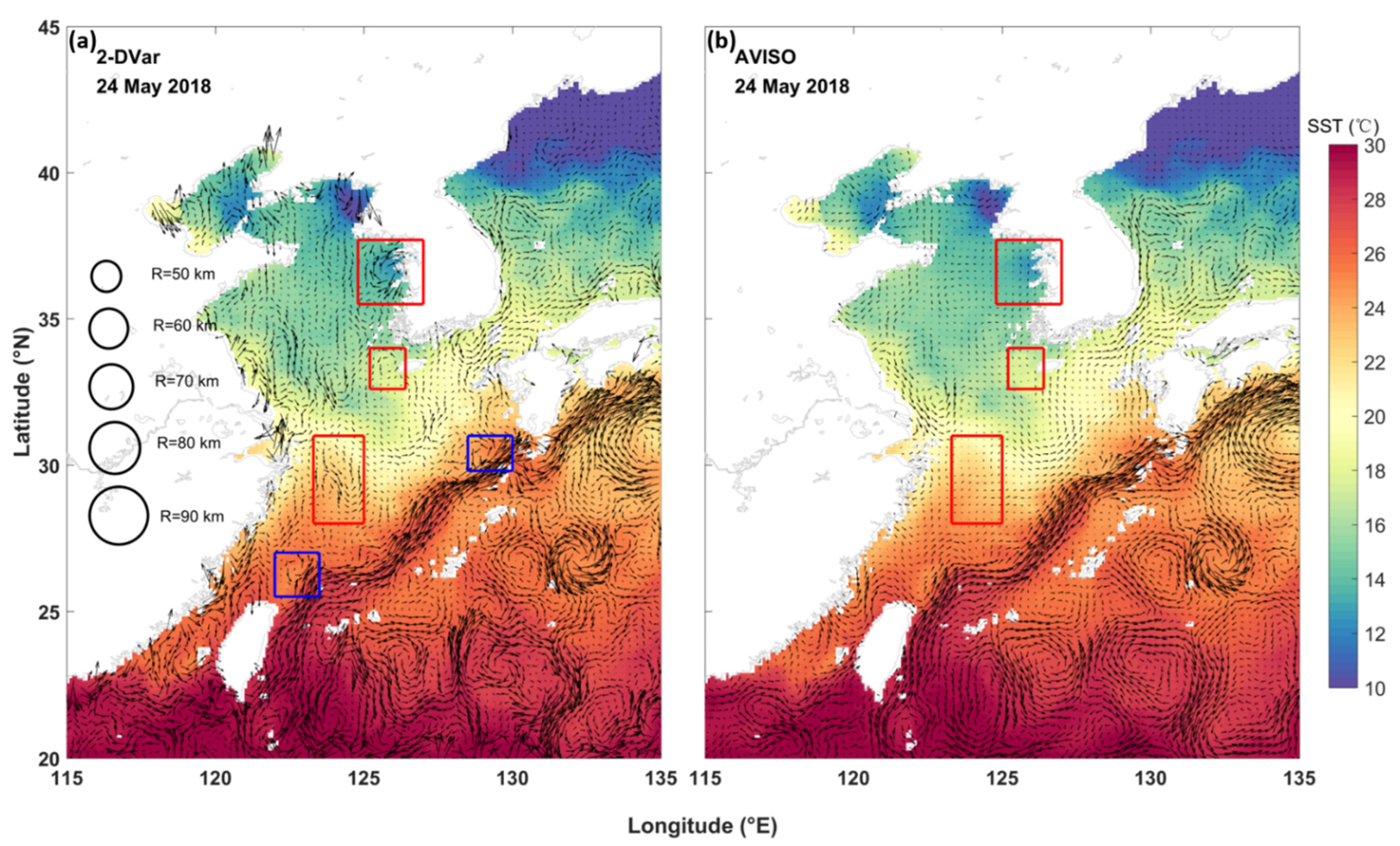
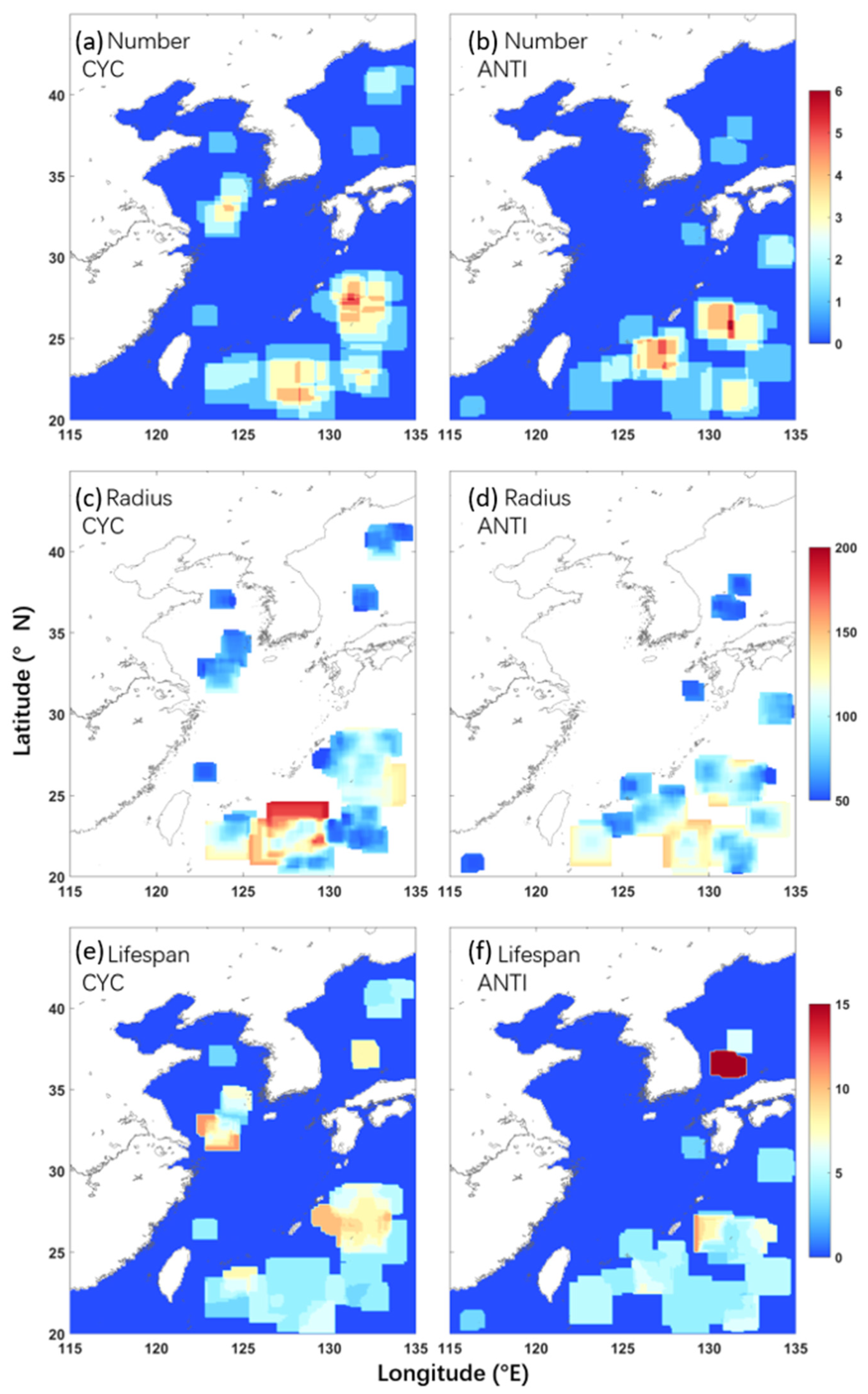
3.3.3. Eddy Detection in the ECS

The ECS is characterized by high eddy activities due to the Kuroshio, complex bathymetry, coastlines and Rossby waves. The eddies are generated locally or move into the ECS from other regions [10,43,44]. As many as 59 eddies are detected in 2-DVar in 2018 (32 cyclonic and 27 anticyclonic eddies). Figure 12a shows the statistics of eddy lifespan. The eddy lifespan in 2-DVar decreases with time, with most eddy lifespans being less than 10 weeks. Previous studies showed a relationship between eddy polarities and eddy lifespan [4,10]. Sangrà et al. [4] showed that anticyclonic eddies accounted for a greater proportion of long-lifespan eddies. In Chen et al. [10], all eddies with a lifespan greater than 30 weeks are anticyclonic. In this study, the only eddy that survives longer than 18 weeks is anticyclonic. Figure 12b shows the statistical results of detected eddy radii. Most cyclonic eddy radii are 50–60 km, while most anticyclonic eddy radii are 50–70 km.

Figure 13a,b shows the spatial distribution of cyclonic and anticyclonic eddies detected from 2-DVar. The densest distribution of eddies is seen in the open ocean, where most mesoscale eddies are generated from Rossby waves propagating from the Pacific. The intrusion of the Kuroshio into the ECS shelf causes cyclonic eddy activities on the northeast side of Taiwan Island. Affected by the topography, the Kuroshio can form anticyclonic eddies on the west side of Kyushu Island and the south side of Shikoku. In addition, several cyclonic eddies are detected in the south Yellow Sea, and both cyclonic and anticyclonic eddies are detected in the Sea of Japan. Figure 13c,d shows the spatial distribution of cyclonic and anticyclonic eddy radii detected from 2-DVar. In general, both cyclonic and anticyclonic eddy radii decrease with latitude. In the open ocean, the mean radii of cyclonic and anticyclonic eddies south of 25°N can be larger than 200 and 150 km, respectively. In the south of the Yellow Sea, the mean radius of cyclonic eddies is about 90 km. In the Sea of Japan, the mean radius of eddies is smaller than 90 km. Figure 13e,f shows the spatial distribution of cyclonic and anticyclonic eddy lifespan detected from 2-DVar. Most lifespans are fewer than five weeks. Eddies with a long lifespan occur in the open ocean. Some cyclonic eddies in the south of the Yellow Sea and the Sea of Japan have long lifespans (about 8 weeks). The only eddy with a lifespan longer than 18 weeks is in the Sea of Japan.

4. Discussion and Conclusions

4.1. Discussion

We analyzed the spatial variability of the 2-DVar performance, and one question is the temporal performance of 2-DVar. In Section 2.2, the geostrophic vorticity evolution is examined and the result shows that the vorticity of 2-DVar displays suitable temporal continuity. We analyze the temporal stability of the 2-DVar by examining the time series of daily RMSE over the mapping domain. Except for a few days when RMSE ranges from 0.04 to 0.06 m, the time series shows values mostly between 0.03 and 0.04 m (Figure 14a). Thus, the daily averaged RMSE does not show a significant trend or temporal variability. To further confirm and illustrate the above observation, we conduct a Fast Fourier Transform (FFT) analysis on the time series of daily averaged RMSE. No significant period is found in the result, indicating that there is no significant period in the time series (Figure 14b). Furthermore, we conduct an FFT on the error time series of each mapping grid and then average the FPSD over the mapping domain. The averaged FPSD does not show a significant period either (Figure 14c). The 2-DVar performance thus shows suitable temporal stability.

We emphasize that the background state should be carefully chosen, and the associated background error covariance should be estimated consistently. However, can the background state and thus the associated background error covariance be further improved to suppress the small-scale errors discussed in Section 2? This study does not discuss observational errors associated with wind-driven and internal tidal signals, which deserve further investigation.

The next issue to discuss is how 2-DVar performs over different areas of the ECS. In the open ocean, the 2-DVar’s performance is satisfactory, with RMSE lower than 0.05 m and correlation higher than 0.95. The mesoscale eddies in the open ocean are relatively large in size and lifespan, and thus can be well reproduced by the 2-DVar. There is an extensive area with high mesoscale eddy activities to the north of Taiwan Island, which are associated with Kuroshio intrusions [45,46]. In this area, it is encouraging that the 2-DVar performance is also satisfactory, with RMSE lower than 0.03 m and a correlation higher than 0.95, and thus, the cyclonic eddies can be well detected. However, there are some challenging areas. In the China-adjacent seas, including the Bohai Sea, the Yellow Sea and the East China Sea, the 2-DVar performance is slightly worse than in the open ocean, as indicated by higher RMSE and lower correlation (Figure 5). Mesoscale eddies detected in this area are few. There are only a small number of cyclonic eddies in the Yellow Sea and the ECS (Figure 13a). In particular, the 2-DVar shows RMSE larger than 0.05 m and a lower correlation below 0.9 along the main axis of Kuroshio. This could be caused by the high-frequency variability of the Kuroshio (Figure 8i). How to improve the performance in these areas requires further investigation.

4.2. Conclusions

In the past two decades, numerous studies have used satellite altimeter data to study mesoscale eddies. Although the widely used AVISO data can satisfy the needs of those studies, its effective resolution imposes limits on research applications at smaller scales. In the present study, a 2-DVar method is implemented for merging altimetry data from five satellites to improve the effective resolutions for the ECS region.

To fully evaluate 2-Dvar, an OSSE based on model simulations is conducted. The OSSE analysis shows that the mean RMSE and correlation of 2-Dvar are 0.035 m and 0.923, respectively. The useful and effective resolution of 2-DVar are about 125 and 210 km, respectively. Furthermore, the frequency–wavenumber analysis shows that the reliable scales of 2-DVar are larger than 210 km in space and longer than 23 days in time.

The results demonstrate that the 2-DVar mapped field has an effective resolution higher than the AVISO mapped field. Furthermore, it has been shown that a higher effective resolution could be obtained, but the background state and the associated background error covariance must be properly and jointly formulated.

The enhanced effective resolution can consequently improve eddy characterization. To quantitatively analyze the eddy characterization capabilities from 2-DVar, we conduct eddy detection. Considering the relationship between the effective resolution and the minimum resolvable eddy radius, $R_{emin}=\frac{1}{4}{\lambda }_x$, eddies with a lifespan of fewer than 23 days and a mean radius smaller than 50 km are discarded. Eventually, 59 eddies are detected in the ECS in 2018, including 32 cyclonic and 27 anticyclonic eddies. The eddies in the open ocean are more numerous, have larger radii and live longer than those in the other area.

References

1. Ducet, N.; Le Traon, P.Y.; Reverdin, G. Global high-resolution mapping of ocean circulation from TOPEX/Poseidon and ERS-1 and -2. J. Geophys. Res. Ocean. 2000, 105, 19477–19498. [Google Scholar] [CrossRef]
2. Pujol, M.I.; Faugère, Y.; Taburet, G.; Dupuy, S.; Pelloquin, C.; Ablain, M.; Picot, N. Duacs dt2014: The new multi-mission altimeter data set reprocessed over 20 years. Ocean Sci. 2016, 12, 1067–1090. [Google Scholar] [CrossRef] [Green Version]
3. Taburet, G.; Sanchez-Roman, A.; Ballarotta, M.; Pujol, M.I.; Legeais, J.F.; Fournier, F.; Faugere, Y.; Dibarboure, G. DUACS DT2018: 25 years of reprocessed sea level altimetry products. Ocean Sci. 2019, 15, 1207–1224. [Google Scholar] [CrossRef] [Green Version]
4. Sangrà, P.; Pascual, A.; Rodríguez-Santana, Á.; Machín, F.; Mason, E.; McWilliams, J.C.; Pelegrí, J.L.; Dong, C.; Rubio, A.; Arístegui, J.; et al. The Canary Eddy Corridor: A major pathway for long-lived eddies in the subtropical North Atlantic. Deep Sea Res. Part I Oceanogr. Res. Pap. 2009, 56, 2100–2114. [Google Scholar] [CrossRef]
5. Swart, N.C.; Ansorge, I.J.; Lutjeharms, J.R.E. Detailed characterization of a cold Antarctic eddy. J. Geophys. Res. Ocean. 2008, 113, C01009. [Google Scholar] [CrossRef]
6. Nan, F.; Xue, H.; Xiu, P.; Chai, F.; Shi, M.; Guo, P. Oceanic eddy formation and propagation southwest of Taiwan. J. Geophys. Res. Ocean. 2011, 116, C12045. [Google Scholar] [CrossRef] [Green Version]
7. Ansorge, I.J.; Lutjeharms, J.R.E. Eddies originating at the South-West Indian Ridge. J. Mar. Syst. 2003, 39, 1–18. [Google Scholar] [CrossRef]
8. Cui, W.; Wang, W.; Zhang, J.; Yang, J. Multicore structures and the splitting and merging of eddies in global oceans from satellite altimeter data. Ocean Sci. 2019, 15, 413–430. [Google Scholar] [CrossRef] [Green Version]
9. Xiu, P.; Chai, F.; Shi, L.; Xue, H.; Chao, Y. A census of eddy activities in the South China Sea during 1993–2007. J. Geophys. Res. Ocean. 2010, 115, C03012. [Google Scholar] [CrossRef] [Green Version]
10. Chen, G.; Hou, Y.; Chu, X. Mesoscale eddies in the South China Sea: Mean properties, spatiotemporal variability, and impact on thermohaline structure. J. Geophys. Res. Ocean. 2011, 116, C06018. [Google Scholar] [CrossRef]
11. Yang, G.; Yu, W.; Yuan, Y.; Zhao, X.; Wang, F.; Chen, G.; Liu, L.; Duan, Y. Characteristics, vertical structures, and heat/salt transports of mesoscale eddies in the southeastern tropical Indian Ocean. J. Geophys. Res. Ocean. 2015, 120, 6733–6750. [Google Scholar] [CrossRef]
12. Zhang, C.; Li, H.; Liu, S.; Shao, L.; Zhao, Z.; Liu, H. Automatic detection of oceanic eddies in reanalyzed SST images and its application in the East China Sea. Sci. China Earth Sci. 2015, 58, 2249–2259. [Google Scholar] [CrossRef]
13. Cui, W.; Yang, J.; Ma, Y. A statistical analysis of mesoscale eddies in the Bay of Bengal from 22–year altimetry data. Acta Oceanol. Sin. 2016, 35, 16–27. [Google Scholar] [CrossRef]
14. Chelton, D.B.; Schlax, M.G.; Samelson, R.M. Global observations of nonlinear mesoscale eddies. Prog. Oceanogr. 2011, 91, 167–216. [Google Scholar] [CrossRef]
15. Escudier, R.; Renault, L.; Pascual, A.; Brasseur, P.; Chelton, D.; Beuvier, J. Eddy properties in the Western Mediterranean Sea from satellite altimetry and a numerical simulation. J. Geophys. Res. Ocean. 2016, 121, 3990–4006. [Google Scholar] [CrossRef] [Green Version]
16. Xu, C.; Shang, X.-D.; Huang, R.X. Horizontal eddy energy flux in the world oceans diagnosed from altimetry data. Sci. Rep. 2014, 4, 5316. [Google Scholar] [CrossRef] [PubMed] [Green Version]
17. Li, Q.; Sun, L.; Xu, C. The Lateral Eddy Viscosity Derived from the Decay of Oceanic Mesoscale Eddies. Open J. Mar. Sci. 2018, 08, 152–172. [Google Scholar] [CrossRef] [Green Version]
18. Liu, Z.; Gan, J. Variability of the Kuroshio in the East China Sea derived from satellite altimetry data. Deep Sea Res. Part I Oceanogr. Res. Pap. 2012, 59, 25–36. [Google Scholar] [CrossRef]
19. Hsin, Y.-C.; Qiu, B.; Chiang, T.-L.; Wu, C.-R. Seasonal to interannual variations in the intensity and central position of the surface Kuroshio east of Taiwan. J. Geophys. Res. Ocean. 2013, 118, 4305–4316. [Google Scholar] [CrossRef]
20. Wu, C.-R.; Hsin, Y.-C.; Chiang, T.-L.; Lin, Y.-F.; Tsui, I.-F. Seasonal and interannual changes of the Kuroshio intrusion onto the East China Sea Shelf. J. Geophys. Res. Ocean. 2014, 119, 5039–5051. [Google Scholar] [CrossRef]
21. Vélez-Belchí, P.; Centurioni, L.R.; Lee, D.-K.; Jan, S.; Niiler, P.P. Eddy induced Kuroshio intrusions onto the continental shelf of the East China Sea. J. Mar. Res. 2013, 71, 83–107. [Google Scholar] [CrossRef]
22. Qiu, B.; Chen, S.; Wu, L.; Kida, S. Wind- versus Eddy-Forced Regional Sea Level Trends and Variability in the North Pacific Ocean. J. Clim. 2015, 28, 1561–1577. [Google Scholar] [CrossRef]
23. Ding, R.; Huang, D.; Xuan, J.; Mayer, B.; Zhou, F.; Pohlmann, T. Cross-shelf water exchange in the East China Sea as estimated by satellite altimetry and in situ hydrographic measurement. J. Geophys. Res. Ocean. 2016, 121, 7192–7211. [Google Scholar] [CrossRef]
24. Ballarotta, M.; Ubelmann, C.; Pujol, M.I.; Taburet, G.; Fournier, F.; Legeais, J.F.; Faugère, Y.; Delepoulle, A.; Chelton, D.; Dibarboure, G.; et al. On the resolutions of ocean altimetry maps. Ocean Sci. 2019, 15, 1091–1109. [Google Scholar] [CrossRef] [Green Version]
25. Kuragano, T.; Kamachi, M. Global statistical space-time scales of oceanic variability estimated from the TOPEX/POSEIDON altimeter data. J. Geophys. Res. Ocean. 2000, 105, 955–974. [Google Scholar] [CrossRef]
26. Kuragano, T.; Kamachi, M. Altimeter’s Capability of Reconstructing Realistic Eddy Fields Using Space-Time Optimum Interpolation. J. Oceanogr. 2003, 59, 765–781. [Google Scholar] [CrossRef]
27. Liu, L.; Jiang, X.; Fei, J.; Li, Z. Development and evaluation of a new merged sea surface height product from multi-satellite altimeters. Chin. Sci. Bull. 2020, 65, 1888. [Google Scholar] [CrossRef]
28. Li, Z.; Zuffada, C.; Lowe, S.T.; Lee, T.; Zlotnicki, V. Analysis of GNSS-R Altimetry for Mapping Ocean Mesoscale Sea Surface Heights Using High-Resolution Model Simulations. IEEE J. Sel. Top. Appl. Earth Obs. Remote Sens. 2016, 9, 4631–4642. [Google Scholar] [CrossRef]
29. Lorenc, A.C. Analysis methods for numerical weather prediction. Q. J. R. Meteorol. Soc. 1986, 112, 1177–1194. [Google Scholar] [CrossRef]
30. Arhan, M.; De Verdiére, A.C. Dynamics of Eddy Motions in the Eastern North Atlantic. J. Phys. Oceanogr. 1985, 15, 153–170. [Google Scholar] [CrossRef] [Green Version]
31. Le Guillou, F.; Metref, S.; Cosme, E.; Ubelmann, C.; Ballarotta, M.; Verron, J.; Le Sommer, J. Mapping altimetry in the forthcoming SWOT era by back-and-forth nudging a one-layer quasi-geostrophic model. J. Atmos. Ocean. Technol. 2020, 38, 697–710. [Google Scholar] [CrossRef]
32. Large, W.G.; McWilliams, J.C.; Doney, S.C. Oceanic vertical mixing: A review and a model with a nonlocal boundary layer parameterization. Rev. Geophys. 1994, 32, 363. [Google Scholar] [CrossRef] [Green Version]
33. Chapman, D.C. Numerical Treatment of Cross-Shelf Open Boundaries in a Barotropic Coastal Ocean Model. J. Phys. Oceanogr. 1985, 15, 1060–1075. [Google Scholar] [CrossRef] [Green Version]
34. Orlanski, I. A simple boundary condition for unbounded hyperbolic flows. J. Comput. Phys. 1976, 21, 251–269. [Google Scholar] [CrossRef]
35. Raymond, W.H.; Kuo, H.L. A radiation boundary condition for multi-dimensional flows. Q. J. R. Meteorol. Soc. 1984, 110, 535–551. [Google Scholar] [CrossRef]
36. Savage, A.C.; Arbic, B.K.; Alford, M.H.; Ansong, J.K.; Farrar, J.T.; Menemenlis, D.; O’Rourke, A.K.; Richman, J.G.; Shriver, J.F.; Voet, G.; et al. Spectral decomposition of internal gravity wave sea surface height in global models. J. Geophys. Res. Ocean. 2017, 122, 7803–7821. [Google Scholar] [CrossRef]
37. Torres, H.S.; Klein, P.; Menemenlis, D.; Qiu, B.; Su, Z.; Wang, J.; Chen, S.; Fu, L.-L. Partitioning Ocean Motions Into Balanced Motions and Internal Gravity Waves: A Modeling Study in Anticipation of Future Space Missions. J. Geophys. Res. Ocean. 2018, 123, 8084–8105. [Google Scholar] [CrossRef] [Green Version]
38. Qiu, B.; Chen, S.; Klein, P.; Wang, J.; Torres, H.; Fu, L.-L.; Menemenlis, D. Seasonality in Transition Scale from Balanced to Unbalanced Motions in the World Ocean. J. Phys. Oceanogr. 2018, 48, 591–605. [Google Scholar] [CrossRef] [Green Version]
39. Nencioli, F.; Dong, C.; Dickey, T.; Washburn, L.; McWilliams, J.C. A Vector Geometry–Based Eddy Detection Algorithm and Its Application to a High-Resolution Numerical Model Product and High-Frequency Radar Surface Velocities in the Southern California Bight. J. Atmos. Ocean. Technol. 2010, 27, 564–579. [Google Scholar] [CrossRef]
40. Dong, C. Oceanic Eddy Detection and Analysis, 1st ed.; Science Press: Beijing, China, 2015; p. 326. [Google Scholar]
41. Dong, C.; Jiang, X.; Xu, G.; Ji, J.; Lin, X.; Sun, W.; Wang, S. Automated Eddy Detection Using Geometric Approach, Eddy Datasets and Their Application. Adv. Mar. Sci. 2017, 35, 439–453. [Google Scholar]
42. Yang, X.; Xu, G.; Liu, Y.; Sun, W.; Xia, C.; Dong, C. Multi-Source Data Analysis of Mesoscale Eddies and Their Effects on Surface Chlorophyll in the Bay of Bengal. Remote Sens. 2020, 12, 3485. [Google Scholar] [CrossRef]
43. Liu, Y.; Dong, C.; Guan, Y.; Chen, D.; McWilliams, J.; Nencioli, F. Eddy analysis in the subtropical zonal band of the North Pacific Ocean. Deep Sea Res. Part I Oceanogr. Res. Pap. 2012, 68, 54–67. [Google Scholar] [CrossRef]
44. Liu, Y.; Dong, C.; Liu, X.; Dong, J. Antisymmetry of oceanic eddies across the Kuroshio over a shelfbreak. Sci. Rep. 2017, 7, 6761. [Google Scholar] [CrossRef] [Green Version]
45. Liu, X.; Dong, C.; Chen, D.; Su, J. The pattern and variability of winter Kuroshio intrusion northeast of Taiwan. J. Geophys. Res. Ocean. 2014, 119, 5380–5394. [Google Scholar] [CrossRef]
46. Liu, Z.; Gan, J.; Hu, J.; Wu, H.; Cai, Z.; Deng, Y. Progress of Studies on Circulation Dynamics in the East China Sea: The Kuroshio Exchanges With the Shelf Currents. Front. Mar. Sci. 2021, 8, 620910. [Google Scholar] [CrossRef]
Figure 1. (a) Study area (115–135°E, 20–45°N) showing the East China Sea and its adjacent areas. The background color is water depth (m), the purple box delineates the sampling area for the wavenumber frequency analysis and the solid red lines are the sampling locations for the time evolution analysis of normalized geostrophic vorticity. (b) Number of times satellite altimeters passed over the region in 2018.
Remotesensing 14 03026 g001
Figure 2. Relationship between background error correlation and distance. The solid blue and yellow lines represent AVISO and 2-DVar, respectively. The dashed yellow line denotes the Gaussian distribution e r 2 / 2 L 2 by fitting 2-DVar with its correlation coefficient scale L of 71 km.
Remotesensing 14 03026 g002
Figure 3. Time evolution of AVISO geostrophic vorticity along (a) Line 1, (c) Line 2 and (e) Line 3 and time evolution of 2-DVar geostrophic vorticity along (b) Line 1, (d) Line 2 and (f) Line 3. The shaded color represents the normalized geostrophic vorticity divided by the local geostrophic parameter. The y-axis is the distance from the sampling line’s southernmost grid point. The gray dots in the 2-DVar figures indicate that there is at least one satellite altimeter observation data. The line graph represents the change rate of normalized vorticity.
Remotesensing 14 03026 g003
Figure 4. (a) Averaged PSD from along-track filtered S3A (black), 2-DVar (blue), 4-Sat (green), 3-Sat (yellow) and AVISO (red). (b) Averaged PSD from along-track filtered S3A (black), averaged PSD from the difference between S3A and 2-DVar (blue), 4-Sat (green), 3-Sat (yellow) and AVISO (red). (c) Averaged PSD ratio of 2-DVar (blue), 4-Sat (green), 3-Sat (yellow) and AVISO (red) to S3A. (d) Averaged PSD ratio of the difference between S3A and 2-DVar (blue), 4-Sat (green), 3-Sat (yellow) and AVISO (red) to S3A.
Remotesensing 14 03026 g004
Figure 5. OSSE 2-DVar dataset (a) RMSE and (b) correlation.
Remotesensing 14 03026 g005
Figure 6. (a) Sampling locations of the spectral analyses, where the red and black lines represent the meridional and zonal sampling lines, respectively. (b) Averaged PSD from CROCO results (red line), OSSE 2-DVar (blue line) and their difference (orange line); (c) PSD ratio of OSSE 2-DVar to CROCO results (SR, blue line) and of their difference from CROCO results (NSR, red line).
Remotesensing 14 03026 g006
Figure 7. Horizontal wavenumber frequency spectral density of SSH in the (a) OSSE 2-DVar and (b) CROCO field. (c) FWPSD score of OSSE 2-DVar.
Remotesensing 14 03026 g007
Figure 8. (a) Mean SSH field; (b) mean large-scale (reliable) SSH and (c) mean SSH noise from CROCO results. (d) Mean SSH field; (e) mean large-scale (reliable) SSH and (f) mean SSH noise from OSSE 2-DVar. (g) Mean absolute difference between CROCO and OSSE 2-DVar SSH fields, (h) low-pass-filtered mean absolute difference and (i) the residual component.
Remotesensing 14 03026 g008
Figure 9. (a) Sum of FPSD over time for 2-DVar (black line) and AVISO (red line); (b) sum of PSD over space for 2-DVar (black line) and AVISO (red line); (c) horizontal wavenumber frequency spectral density of ADT in 2-DVar; and (d) horizontal wavenumber frequency spectral density of ADT in AVISO.
Remotesensing 14 03026 g009
Figure 10. Comparison of the geostrophic current field (vectors) and SST (shaded, °C) on 24 May 2018 between (a) 2-DVar and (b) AVISO. The red boxes in the two figures denote identified small-scale structures that AVISO does not resolve compared to 2-DVar. The blue boxes denote identified “anomalous” small-scale structures in 2-DVar. The black circles illustrate eddy sizes with radii of 50 to 90 km.
Remotesensing 14 03026 g010
Figure 11. (a) Ideal ADT field, where the shaded color represents the normalized ADT; (b) ADT along the black line in a; (c) schematic of the geostrophic current field derived from the ADT field in a; and (d) normalized geostrophic velocity of (c), where the shaded color represents the normalized geostrophic velocity and the black line represents the position of the ADT in (b).
Remotesensing 14 03026 g011
Figure 12. Histograms of (a) eddy lifespan, where “>20” represents the total number of eddies with a lifespan greater than 20 weeks and (b) eddy radii, where “>90” represents the total number of eddies with a radius larger than 90 km.
Remotesensing 14 03026 g012
Figure 13. Distributions of (a) cyclonic and (b) anticyclonic eddy number. (c) Mean cyclonic and (d) anticyclonic eddy radius (km). (e) Cyclonic and (f) anticyclonic eddy lifespan (week) detected in 2-DVar. The eddy number (eddy radius, eddy lifespan) in each grid (0.08 degree) is the total number of times (mean radius, mean lifespan) an eddy is detected in that grid.
Remotesensing 14 03026 g013
Figure 14. (a) Time series of daily averaged RMSE. (b) FPSD of daily averaged RMSE. (c) Averaged FPSD of errors of each grid.
Remotesensing 14 03026 g014