Article

Evidence of Ocean Waves Signature in the Space–Time Turbulent Spectra of the Lower Marine Atmosphere Measured by a Scanning LiDAR

Nantes Université, École Centrale Nantes, CNRS, LHEEA, UMR 6598, F-44000 Nantes, France
*
Author to whom correspondence should be addressed.
Remote Sens. 2022, 14(13), 3007; https://doi.org/10.3390/rs14133007
Submission received: 11 May 2022 / Revised: 15 June 2022 / Accepted: 15 June 2022 / Published: 23 June 2022

Abstract

:
To achieve more accurate weather and climate forecasting, and propose efficient engineering solutions for exploiting offshore renewable energies, it is imperative to accurately describe the atmospheric turbulent flow in the offshore environment. The ocean’s dynamics raise specific challenges for the aforementioned applications, as they significantly alter the atmospheric flow through complex wind–wave interactions. These interactions are important in fairly common situations and notably in old-sea conditions, where ocean waves travel fast, under comparatively slow wind velocities. In the present study, a scanning LiDAR (sLiDAR) was deployed on the shore to study micro-scale wind–wave interactions by performing horizontal scans 18 m above the ocean, and as far as 2 km from the coast. In the proposed configuration, and in the test cases presented in old seas, the sLiDAR captures wave-induced disturbances propagating into the lower part of the marine atmospheric boundary layer. Based on measurements of high-resolution space–time maps of the Radial Wind Speed, an original two-dimensional spectral analysis of the space–time auto-correlation functions was performed. Unlike more conventional data-processing techniques, and as long as the waves travel sufficiently (∼twofold) faster than the mean wind at the measurement height, the upward transfer of motions from the waves to the wind can be clearly distinguished from the atmospheric turbulence in the wave-number–angular-frequency (kw) turbulent spectra. These are the first space–time auto-correlation functions of the wind velocity fluctuations obtained at micro-scales above the ocean. The analyses demonstrate sLiDAR systems’ applicability in measuring kw-dependent turbulent spectra in the coastal environment. The findings present new perspectives for the study of micro-scale wind–wave interactions.

1. Introduction

The Marine Atmospheric Boundary Layer (Marine ABL, or MABL) is often subject to significant wave-induced (WI) disturbances governing wind–wave interactions above the ocean. Despite the many studies that have been conducted since the pioneering theoretical works of [1,2,3,4,5], modern experimental campaigns such as those exploited in [6,7,8,9,10], and the high-fidelity numerical simulations, performed, e.g., by [11,12,13,14,15], in many respects, how the waves disturb the atmospheric flow in the offshore environment remains unclear. Most experimental studies adopt a consequential approach, in which the waves’ influence is often observed by mean wind and turbulent profiles’ deviation from in-land predictions (Monin–Obukhov Similarity Theory, MOST [16,17,18]) in the inner part of the MABL [6,19], and the sea-state dependence of the drag coefficients affecting the flow above that region [9,20].
According to theory [3,5], and observations [7,8], WI disturbances extend into limited regions above the free surface. A commonly adopted consequential strategy is to define the air-side of the wave boundary layer (WBL) as the region in which the wind or turbulent profiles strongly deviate from widely accepted in-land similarity theories [21]. A problem is that wind–wave interactions involve multiple physical mechanisms, propagating up to different heights and disturbing different quantities in the MABL. Moreover, standard similarity theories such as MOST often fail due to the lack of homogeneity and steadiness in the atmosphere [22]. Together with measurement-induced bias, these problems introduce significant uncertainty to the determination of a WBL height.
The definition of the WBL relates to the existence of a WI flow, i.e., ocean wave dynamics (c.f. [23,24,25,26]) that propagate into the atmosphere and are subjected to significant wind–wave interactions [5,27]. Similarly to turbulence and WI motions, ocean waves are commonly described by an energy spectrum [23]. In the atmosphere, turbulent kinetic energy is generated at large energetic scales, and then transferred to small scales, where it can be dissipated by viscous forces, in a process known as the Kolmogorov energy cascade [28]. In the ocean, a spectral energy cascade such as Kolmogorov’s is sustained due to non-linear wave–wave interactions and, at small scales, the sea-state spectrum saturates due to wave-breaking processes [24]. In the marine environment, wave and wind dynamics are closely related to each another in terms of their spectral similarity [25,26]. Therefore, a transfer function exists between ocean waves and the consequent WI motions in the atmosphere [5,27].
The WI flow is assumed to be significant in the WBL, and is the origin of other WI disturbances that propagate farther above in the MABL. However, a more precise definition of the WBL and the WI flow remains elusive, as the significance of the WI disturbances is often dependent on the variables of interest [7]. To improve the phenomenological comprehension of WI disturbances in the atmosphere, the present work adopts a mechanistic (c.f. [7]) rather than a consequential approach. In this regard, we aim to assess WI velocities directly, rather than to infer WI disturbances from wind velocity profiles [13,29,30,31], total momentum fluxes [9,10,14,32], or turbulent kinetic energy (TKE) budget analyses [19,33,34,35].
From a mechanistic perspective, the WI flow is often observable in frequency (f)-dependent turbulent spectra through a pronounced increase in the spectral energy distribution at the wave predominant frequencies. This phenomenon was first encountered in [36], that provide experimental evidence of WI disturbances in the spectra of velocity and humidity fluctuations above the Caspean Sea. WI pressure fluctuations were earlier detected above the ocean in the Bahamas, through air-pressure sensors in [37]. In more recent campaigns, sonic anemometers were used to detect WI disturbances in the velocity fluctuations and their derived quantities, e.g., in [8,27,38]. Nevertheless, many attempts to detect WI disturbances in the frequency-domain turbulent spectrum have failed [7].
Alternatively, multiple turbulent sources can be observed traveling with different velocities in the space–time domain. In the atmosphere, turbulent motions are generally convected by the mean velocity U, and tend to follow Taylor’s hypothesis, so that the angular-frequency (w) and wave-number (k) of a turbulent eddy are related as w = k U [39,40]. On the other hand, ocean wave components propagate at phase velocity c ( k ) = w ( k ) / k , and transport energy forward at group velocity c g = w / k , which are both determined in a linear wave theory framework (c.f. [41,42,43]) from the characteristic dispersion equation w 2 = k g tan h ( k d ) , with g the gravity and d the water depth. Based on the analysis of a two-dimensional (2D) wave-number–angular-frequency (kw)-dependent turbulent spectrum E ( k , w ) , the characterization of atmospheric turbulence and WI motions propagating with different velocities (U and c p ) is noted within a numerical framework in [15]. A few measurements of the ocean wave elevation spectrum were conducted in the kw space [44,45], but none were found to provide access to the kw turbulent spectrum at similar scales in the MABL.
Kolmogorov’s turbulent cascade was developed for the k-dependent turbulent spectrum [28], and most experimental campaigns provide access to f-dependent spectra in the ABL [8,27,37,38]. While several studies have addressed one-dimensional (1D), k- or f-dependent turbulent spectra, few have investigated the 2D kw spectrum, even in flat-bottom conditions. There is no universally accepted model for the kw turbulent spectrum in simple shear flows. The first, and most widely explored, model for the kw turbulent spectrum was proposed by Taylor [39], who puts forward the frozen turbulence hypothesis. In the literature concerning atmospheric flows, it is common to assume Taylor’s hypothesis (c.f. [46]) to transform between k- and f-dependent spectra, or between space and time characteristic flow scales. In the kw domain, Taylor’s hypothesis corresponds to a straight line, which contrasts with the continuous distributions observed in nature, as the energy density function (EDF) spreads in the vicinity of this linear prediction. The concept of spreading leads to the random sweeping hypothesis, which was exploited earlier in [47], and later, e.g., in [40,48,49]. A state-of-the-art review of these kw spectrum models is presented in [49].
Here, the wave influence in the MABL was investigated within the WBL through original field measurements taken by a scanning Light Detection and Ranging (sLiDAR) system employed on the coast. The sLiDAR-specific literature review ([50,51,52,53,54,55,56,57,58]) is presented in Section 2.2.1. Operating in staring mode, i.e., staring in a single direction with fixed line of sight (LOS), the sLiDAR registers highly detailed space–time mappings of the radial wind speed (RWS), here approximating the longitudinal wind velocity. With fine space–time discretizations in similar ranges and uniform grids, this provides access to the 2D kw turbulent spectrum measured 18 m above the ocean.
The sLiDAR was employed in the test site described in Section 2.1, and operates according to the experimental setup described in Section 2.2. Meteocean-monitoring strategies are presented in Section 2.3. Appendix A presents the techniques employed to identify and reconstruct poor-quality data, while the most significant results are based on the spectral analyses described in Section 3.1. Through these observations, WI motions are revealed by space–time maps of the RWS in Section 4.1, 1D k- or f-dependent spectra in Section 4.2, and 2D kw-dependent spectra in Section 4.3. Cases with vanishing wave signatures are presented for comparison in Section 4.4.

2. Experimental Campaign
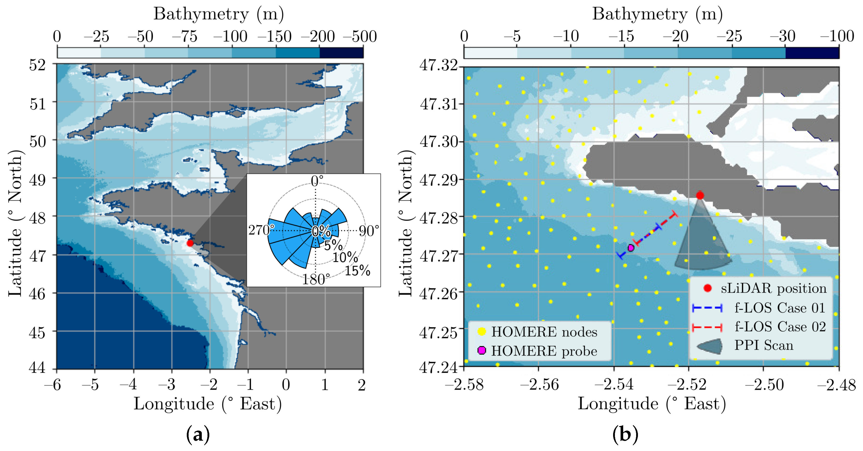
2.1. Test Site

From October 2020 to January 2021, the sLiDAR, Leosphere WindCube® Scan 100S depicted in Figure 1, from the research laboratory in Hydrodynamics, Energetics and Atmospheric Environment (LHEEA), was deployed to explore micro-scale wind–wave interactions close to the water surface by performing horizontal scans at a height of 18 m above the mean sea level (MSL). The sLiDAR was installed 100 m from the coastline in the peninsula of Le Croisic (France), on the balcony of a seafront villa with a clear view to the North Atlantic ocean from 135° to 260°. The location of Le Croisic is shown in Figure 2a, with the wind rose obtained for 2008–2017 from [59], giving the prevailing wind direction (WD) of south-west and north-east. The test site is mostly a suburban area, composed of low-rise buildings and parks with a south-western rocky coastline, aligned with an 110°–290° axis for nearly 10 km, as pictured in Figure 2b. Directly to the north-east of the sLiDAR’s position (47°17 8.6 N, −2°31 1.5 E), the Penn-Avel park is a densely forested area with tall vegetation of approximately 10 m in height. The local ground is around 8 m above the MSL with a mean slope of 8% down to the water in the south-west direction.

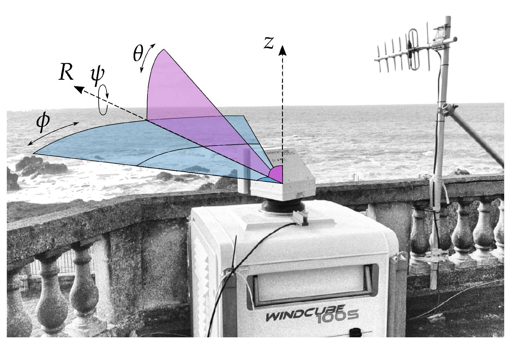
2.2. sLiDAR Technology and Experimental Setup

2.2.1. Technology and Challenges

Driven by the growth in remote-sensing applications for weather forecasting and wind energy exploitation, LiDAR technologies and post-processing techniques have experienced a rapid growth over the last 20 years. A wide range of applications are referred to in [50], including weather and climate monitoring and forecasting (c.f. [51,52]), fundamental studies in turbulent flows and the ABL (c.f. [53,54]), and many studies concerning the wind energy industry (c.f. [55,56]). As the latter is now moving to the offshore environment, LiDAR applications that are performed offshore are also encountered [57].
The present experimental setup poses two challenges that are particularly important for the subsequent analyses, i.e., mitigating the bias induced by the misalignment between WD and the sLiDAR’s LOS, and evaluating the laser volume-filtering effect [50]. Due to misalignment, the turbulent spectrum measured along the LOS is contaminated by various components of the spectral tensor, i.e., a second-order tensor that contains the full directional information of the EDF (or turbulent spectra). For this reason, sLiDAR-aligned wind conditions were selected in this study, to enable a comparison between the present observations and the commonly addressed longitudinal correlations/spectra.
The filtering effect is observed through the mitigation of small-scale turbulent motion and is generally flow-dependent. sLiDAR measurements are often compared to measurements performed with other instruments, such as sonic anemometers, to evaluate or correct the sLiDAR filter-induced bias [58]. The setup employed here was not equipped with such instrumentation and, to the authors’ knowledge, no other physical experiment has been performed to assess space–time velocity correlations in similar scales above the ocean. A kw dependent bias is therefore expected in the turbulent spectra, but its implications for the joint space–time correlation functions are as yet unreported in the literature. This bias is further discussed in the results section (Section 4).

2.2.2. Calibration and Configuration

The sLiDAR azimuth and elevation angles were determined using the classical hard target procedure [60], leading to an uncertainty of less than 0.5°. Using the sLiDAR internal inclinometers, pitch ( θ ) and roll ( ψ ) angles, defined in Figure 1, were adjusted to values with an uncertainty below 0.1°. For the azimuth of 221.8° with zero elevation employed in this study, this misalignment leads to an angle of elevation offset of 0.07° pointing down to the water surface, corresponding to an altitude offset of −1.1 m per kilometer distance from the sLiDAR’s position. Tidal variations during the presented test cases led to an uncertainty of 2 m on the sLiDAR altitude above the actual sea level.
In order to assess the time and space spectral content of the wind velocity fluctuations, the sLiDAR was set up in staring mode with an elevation angle θ = 0°, measuring the RWS ( u R ) along a horizontal fixed LOS (f-LOS) approximately 18 m above the MSL. The RWS is negative when the wind blows towards the sLiDAR in the f-LOS direction. During the measurement campaign, the acquisition frequency ranged from 1 Hz to 4 Hz and the acquisition time was set to 600 s for each f-LOS scan. Gates were defined at each 10 m along a 1 km LOS, starting at least 0.75 km away from the sLiDAR position. Considering that the gate length was set to L γ = 25 m, which is the smallest value available on this device, that provides a 60% gate overlapping. As the comparison between time and space data is easier to interpret when the wind is aligned to the f-LOS, an azimuth angle ϕ L = 221.8° was chosen, in agreement with the prevailing wind sectors and wave directions at Le Croisic (Figure 2a).
To monitor the WD close to the area of measurement, horizontal Plane Position Indicator (PPI) scans with 45° opening and θ = 0° were performed for a duration of 16 s, within a 96 s pause between each 10-min f-LOS scan. The RWS registered in these PPI scans was processed along the gates following the velocity volume processing method described in [60], obtaining gate-wise horizontal wind speed (WS) and WD. This method uses a cosine fitting function and assumes that the wind field is homogeneous in time and space during each PPI scan, which seems particularly appropriate in offshore conditions [60]. The WS and WD shown in Section 2.3 were averaged over the 51 gates and 1.25 km along the PPI LOS sector.
The different staring mode and PPI scans are depicted in Figure 2b. Details of the configuration used for these scans are given in Table 1.

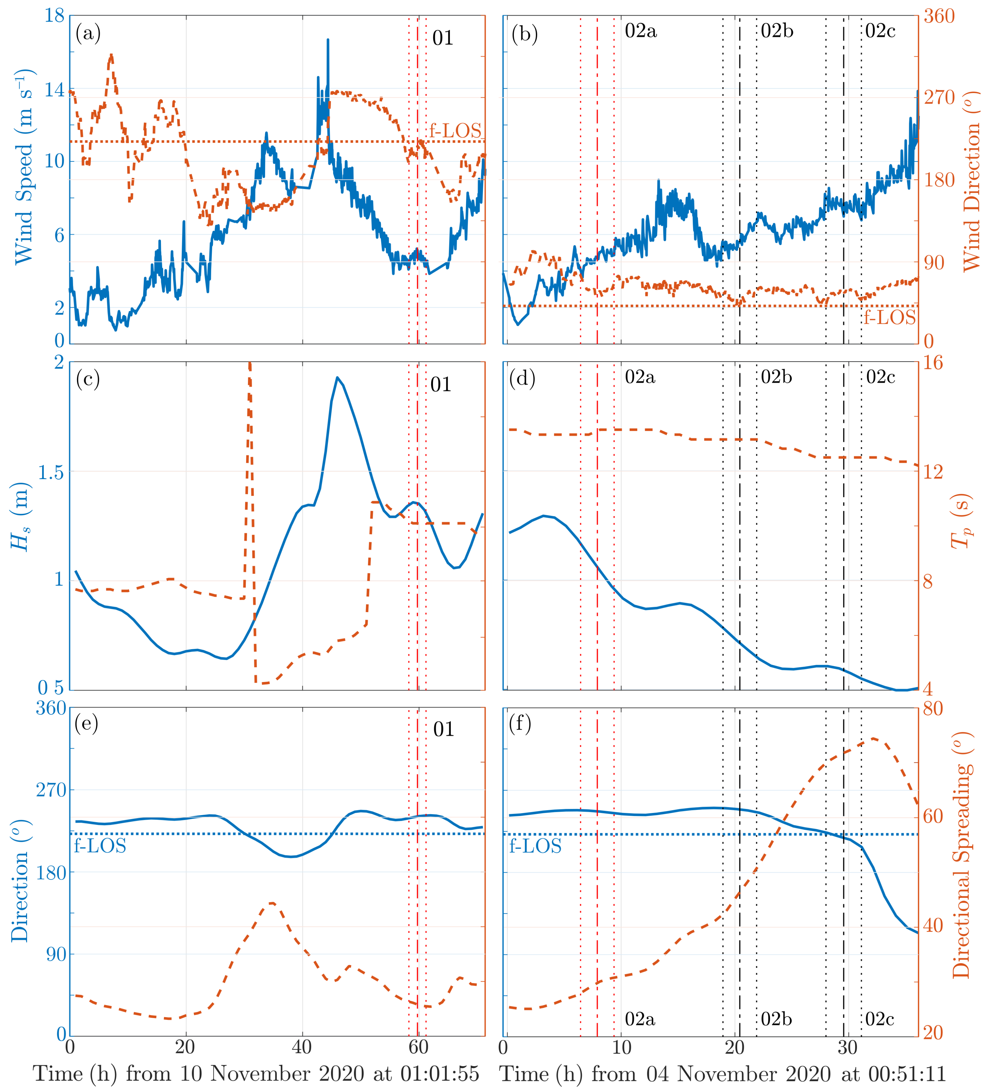
2.3. Environmental Description and Test-Case Selection

2.3.1. Meteocean Conditions

The horizontal WS and WD were monitored using the sLiDAR PPI scans described in Section 2.2. The turbulence intensity (TI) was averaged between various f-LOS scans defining a 3-h test case, and was computed as
T I = u R u R ¯ u R ¯ 2 ,
where u R = u R u ¯ R is the RWS fluctuation, with · ¯ the space–time average operator, and · the ensemble average (between 10-min f-LOS scans) operator. The total average RWS is U R = < u ¯ R > .
The atmospheric thermal stability was estimated on a 3-h basis using the bulk Richardson number R i b (c.f. [61]), here defined by assuming the Boussinesq approximation for incompressibility (c.f. [62]), as seen, for example, in [63]:
R i b = β θ g Δ T z U R 2 ,
where β θ = 3.4 · 10 3 ( 1 / °C) is the coefficient of thermal expansion, z = 18 m is the measurement height, and Δ T = T a i r − SST is the air–sea temperature difference. The air temperature T a i r was recorded by a pressure–temperature–humidity (PTH) probe on the balcony near the sLiDAR, and the sea surface temperature (SST) came from the MARC database using the MARS3D model [64].
Due to the lack of available concomitant measurements at sea during the sLiDAR campaign, it was decided to exploit sea-state parameters from a modeling chain whose performances have already been extensively characterized in the area. The HOMERE hindcast database [65], a highly refined setup covering the whole Bay of Biscay and Channel sea, was used for the needs of this campaign. It is based on a WAVEWATCH III (WWIII) set-up running on an unstructured grid, with a characteristic resolution ranging from 200 m to 10 km. Three long-term moorings of Datawell wave buoys are deployed in the area, from roughly 15 to 55 km away from the sLiDAR measurement, in water depths ranging from 12 to 56 m. This provides a good reference in terms of uncertainties associated with the use of model data. Significant wave height, for instance, is estimated in a range from 12 to 14% of the normalized root-mean-square error, and from 2 to 3% normalized bias for the three buoys [66,67]. The global sea-state parameters, i.e., the significant height H s , peak wave length L p , peak period T p , mean wave direction α w , and wave directional spread β w , were extracted hourly at the node closest to the sLiDAR f-LOS final gate, from the numerical grid of HOMERE depicted in Figure 2b.
The water depths were also extracted from HOMERE. The mean depth ranged from d 14 m close to the first f-LOS gate, to d 22 m close to the last f-LOS gate. The tidal range in the area reaches 6.16 m referenced at Le Croisic harbor by SHOM, the French hydrographic service, and the tidal regime is semi-diurnal. Although tides imply variations in both depth and relative height between the water surface and the sLiDAR measurement, tidal variations in water surface elevation occur in such large space–time scales that their effect does not interfere with the spectral analyses presented here. The highest water level variation that occurred during the experiment was approximately ±2 m around MSL. The water depth evaluation in Section 4.3 was, therefore, considered in a range that accounts for its variation in space and time at the scales of the sLiDAR measurements.
The wave age (WA) is here defined as WA = c p / U R , a function of the estimated peak wave phase velocity c p = L p / T p and the f-LOS-measured RWS. U R is negative when the wind comes from the ocean; hence, when the wind and wave directions are aligned, WA > 0 . A negative WA value highlights the intrinsic difference concerning the less understood wind–wave interaction mechanisms of wave-opposed wind situations where U R > 0 .

2.3.2. Test Cases

Two date periods (from 10 to 12 November 2020, as 10:12-Nov; and from 4 to 5 November 2020, as 4:5-Nov) are presented here, from which four cases (01, 02[a–c]) were selected for further evaluation. The presented periods indicate the presence of a swell, i.e., long energetic wave trains generated far out in the ocean and usually characterizing old-sea conditions. The important difference between these dates is the WD, which came from the ocean on 10:12-Nov (Case 01), and from the land on 04:05-Nov (Cases 02[a–c]). The main wind and sea-state statistics of the cases are summarized in Table 2 and Table 3.
The most important meteocean variables monitored in each date period are presented in Figure 3. Those characterizing the wind, WS and WD are reconstructed in (a) and (b); regarding the sea-state, H s and T p are shown in (c) and (d), while α w and β w are plotted in (e) and (f). The date periods 10:12-Nov and 04:05-Nov are indicated, respectively, (left) in Figure 3a,c,e, and (right) in Figure 3b,d,f. The 3-h periods selected for further exploitation stand between the vertical (Red for Case 01 and 02a; black for Cases 02[b,c]) dashed lines, and the middle time is denoted in vertical dot-dashed lines. The horizontal lines in Figure 3a,b,e,f stand for the f-LOS direction.
The cases were selected to obtain the best alignment of the f-LOS direction ([221.8°, 41.8°]) with the mean wind and wave directions. Case 01 is one of the few possibilities on 10:12-Nov, but a wide range of possibilities were available on 04:05-Nov thanks to the mostly constant WD that was registered, leading to Cases 02[a–c]. According to Table 2, the misalignment of the mean WD to the sLiDAR f-LOS was nearly 10° for Case 01 and 18° for Case 02a, leading to a RWS to WS ratio of 99% and 95%, respectively. Cases 01 and 02a were characterized by a similar WA magnitude (|WA|), which significantly dropped through Cases 02b and 02c in a diminishing swell and increasing WS scenario.
Cases 01 and 02[a–c] are intrinsically different due to the 180° shift in WD, and the different stability regimes. Case 01 registered a wave-following wind scenario, with a comparatively large fetch from the open ocean, where wind–wave interactions could better approach a dynamic equilibrium state. In contrast, Cases 02[a–c] registered wave-opposing wind scenarios with the wind coming from the land, and only ∼1 km of ocean fetch. Impacted by in-land non-homogeneity and unstable stability regimes, Cases 02[a–c] are, therefore, characterized by stronger turbulence intensities. Case 01 and Case 02a have comparable |WA|, but Case 01 presents a higher (129% ratio) significant height H s , with a lower (75% ratio) peak period T p . Consequently, the sea-state energy flux (in deep waters proportional to H s 2 T p ) is expected to be approximately 25% higher in Case 01.

3. Data Treatment and Analyses

The following refers to the post-processing techniques used to evaluate the staring mode dataset of the RWS. The dataset corresponds to measurements performed during the 3-h test cases described in Section 2.3.2, and is segmented into 9 samples of 10-min records.
sLiDAR measurements may be sensitive to the atmospheric conditions that control the particle density in the ABL, and become improper, for example, through an insufficient concentration of particles, or due to the ray collision with hard targets [68,69,70,71]. For that reason, it is imperative to properly identify and treat outliers in the measurements. The data quality and filter techniques that were employed have a limited impact on the main contributions, and are, therefore, described in the Appendix A.

3.1. Energy Density Functions

Aligning the sLiDAR f-LOS as close as possible to the WD in a quasi-steady wind condition, it is here assumed that the RWS ( u R ) approximates the streamwise component of the wind velocity ( u 1 ). The distance r is measured along the f-LOS approximating the streamwise distance. The presented spectra are, therefore, approximations of the longitudinal spectra E u 1 u 1 E u R u R . Any deviation between wind and f-LOS directions contaminates the spectra with the full spectral tensor information [50].
The space–time auto-correlation function (c.f. [40,49]) of u R is computed from its definition:
R u R u R ( r , τ ) = u R ( x , t ) u R ( x + r , t + τ ) ¯ ,
and the corresponding spectral EDF (or turbulent spectrum) E u R u R ( k , w ) is obtained from its Fourier Transform (FT). They therefore form Fourier Pairs, as in:
E u R u R ( k , w ) = 1 ( 2 π ) 2 R u R u R ( r , τ ) e i ( k r + w τ ) d r d τ , and R u R u R ( r , τ ) = E u R u R ( k , w ) e + i ( k r + w τ ) d k d w ,
with k = 2 π / r , and w = 2 π / τ = 2 π f . Further details on the 2D FT are given in Section 3.2.
More commonly available in the literature, the one-dimensional space and time spectra E u 1 u 1 ( k ) and E u 1 u 1 ( w ) , form Fourier pairs with the one-dimensional correlation functions R u 1 u 1 ( r ) and R u 1 u 1 ( τ ) , respectively. Inside a 10-min series, R u R u R was averaged in space and time. This led to nine samples of E u R u R per case, from which the ensemble average spectrum was computed.
Because the 2D wave-number–angular-frequency spectrum can be considerably more noisy than the 1D spectra, and since the turbulent eddies convected by the mean wind velocity crossed the LOS 1 km span in much less than 10-min (3.33 min if u R ¯ 5 m s 1 ), the dataset was further segmented prior to the computation of the 2D spectrum. To obtain the total averaged 2D spectrum, each of the nine 10-min series was segmented into three: R u R u R ( r , τ ) was averaged inside a 3.33-min space–time series, and the ensemble average of E u R u R ( k , w ) was performed over 27 segments of 3.33-min.

3.2. Two-Dimensional Fourier Transform

The 2D FT of the generic variable χ ( r , τ ) gives the approximation of χ in the wave-number–angular-frequency dimensions:
χ ( r , τ ) = Q 0 + 0 0 Q ( k , w ) e i ( k r w τ ) + Q + ( k , w ) e i ( k r + w τ ) + Q + ( k , w ) e i ( + k r w τ ) + Q + + ( k , w ) e i ( + k r + w τ ) d k d w .
Employing Equation (5), the signal χ ( r , τ ) is linearly decomposed into all the existing harmonics of k and w modal spaces. In a discrete formulation, one refers to the Discrete FT (DFT). Determining the complex-valued Fourier coefficients Q ± ± ( k , w ) of the DFT requires a Fast Fourier Transform (FFT) algorithm. The 2D (D)FT is separable, so that a 2D FFT is obtained from multiple one-dimensional FFTs, acting sequentially in k and w directions. It is also conjugate fold-symmetric, meaning that Q = Q + + * and Q + = Q + * , as the superscript · * , stands for the complex conjugate operator. Here, the EDF is computed from an auto-correlation function of velocity fluctuations ( χ R u R u R ), so Q ± ± ( k , w ) is real, the average contribution Q 0 is null, and the 2D FT is fold-symmetric.
In contrast to Equation (4), Equation (5) distinguishes the contribution of positive, and negative, wave-numbers and angular-frequencies to the transformation. This decomposition leads to the definition of a four-quadrant spectrum, which considering the EDF of R u R u R as in Equation (4), becomes:
Q ± ± ( k , w ) = 1 ( 2 π ) 2 R u R u R ( r , τ ) e i ( ± k r ± w τ ) d r d τ , with E u R u R ( k , w ) = 2 ( Q + Q + )
The physical meaning of positive and negative wave-number and angular-frequency scales is rather dubious, and is further discussed in Section 4.3.2. Otherwise, with Equation (6), the resultant EDF E u R u R ( k , w ) exploited in Section 4.3.1 is uniquely defined as a function of positive k and w. The integration of E u R u R ( k , w ) in (positive) k or w domains, leads to the single-sided, one-dimensional spectra usually encountered in the literature.

4. Results

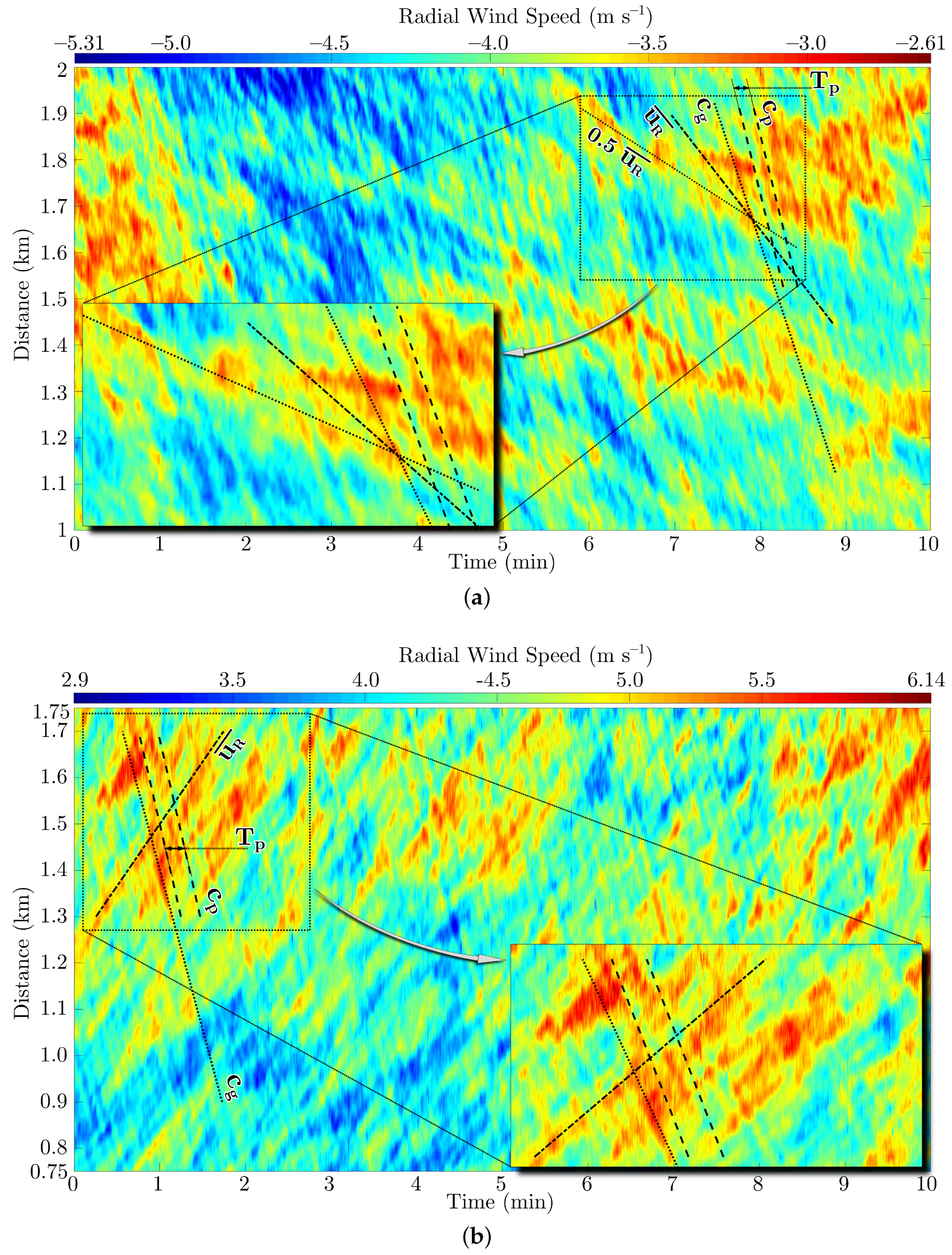
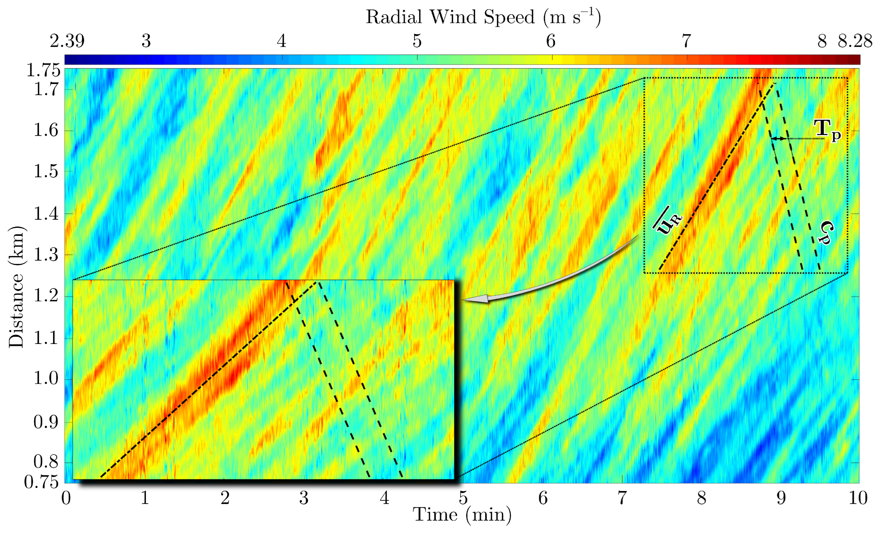
4.1. Radial Wind Speed Fluctuations

The existence of coherent vortical structures in turbulent flows is usually revealed by the observance of consequent turbulent streaks, i.e., coherent patterns of alternating velocities, depicting the presence of a turbulent eddy [72]. These turbulent streaks are usually identified in the ABL by examining 2D space mappings of the longitudinal (x) velocities, captured in either the xy or the xz planes. Alternatively, color plots of the spatio-temporal RWS registered in f-LOS (10-min) records are presented for Case 01 in Figure 4a, and for Case 02a in Figure 4b.
Also in the spatio-temporal map, one encounters alternating low- and high-speed regions depicting an atmospheric turbulent streak. Instead of providing two spatial dimensions of the streak, a spatio-temporal map identifies its (approximately) longitudinal dimension (span in the vertical axis), and duration (span in the horizontal axis). A spatio-temporal map also depicts the apparent transport velocity of these atmospheric streaks, which is identified by the slopes drawn in Figure 4 and discussed below.
According to Taylor’s hypothesis, in a flat-bottom scenario, the turbulent eddies are convected by the local mean speed. To evaluate this in the sLiDAR f-LOS, the mean RWS of the 10-min period is shown as dot-dashed lines in Figure 4. The agreement between the space–time evolution of large atmospheric streaks and Taylor’s hypothesis is clearly seen in Case 02a in Figure 4b. This is less clear, however, for Case 01 shown in Figure 4a. Instead, the streaks in Case 01 appear to be convected by lower velocities than the RWS. The arbitrary value 0.5 RWS shown in dotted lines in Figure 4a is provided as a reference to guide the discussion in Section 5.1.
In contrast, WI motions propagate with similar properties to those of the sea surface, and thus follow the dispersion equation that imposes the (peak) wave phase and group velocities ( c p and c g ), given in Table 3 and also depicted in Figure 4. Particularly important at small scales, the phase velocity c p is indicated by two dashed lines, separated by T p . At larger scales, at the order of the sLiDAR range, the wave modulation by envelopes traveling with c g (dotted line) could theoretically take over as the predominant feature in space–time mappings of the sea-surface displacements. Nonetheless, one can note that the intermediate-to-shallow depths at play in this experiment are such that c g > 0.75 c p , approaching the slopes of c p and c g in Figure 4. As a result, their effects are almost indistinguishable from one another in view of the predominant turbulent behavior of the RWS fluctuations.
For each case presented in Figure 4, the atmospheric streaks are consistently deformed by the WI flow and, therefore, hatched by slopes that qualitatively correspond to c p and c g , and separated by periods approximating T p . The close relation between space–time RWS fluctuations and wave characteristics suggests that, at the measurement height, a significant portion of the wave motions is transferred to the wind, in the form of WI RWS fluctuations.

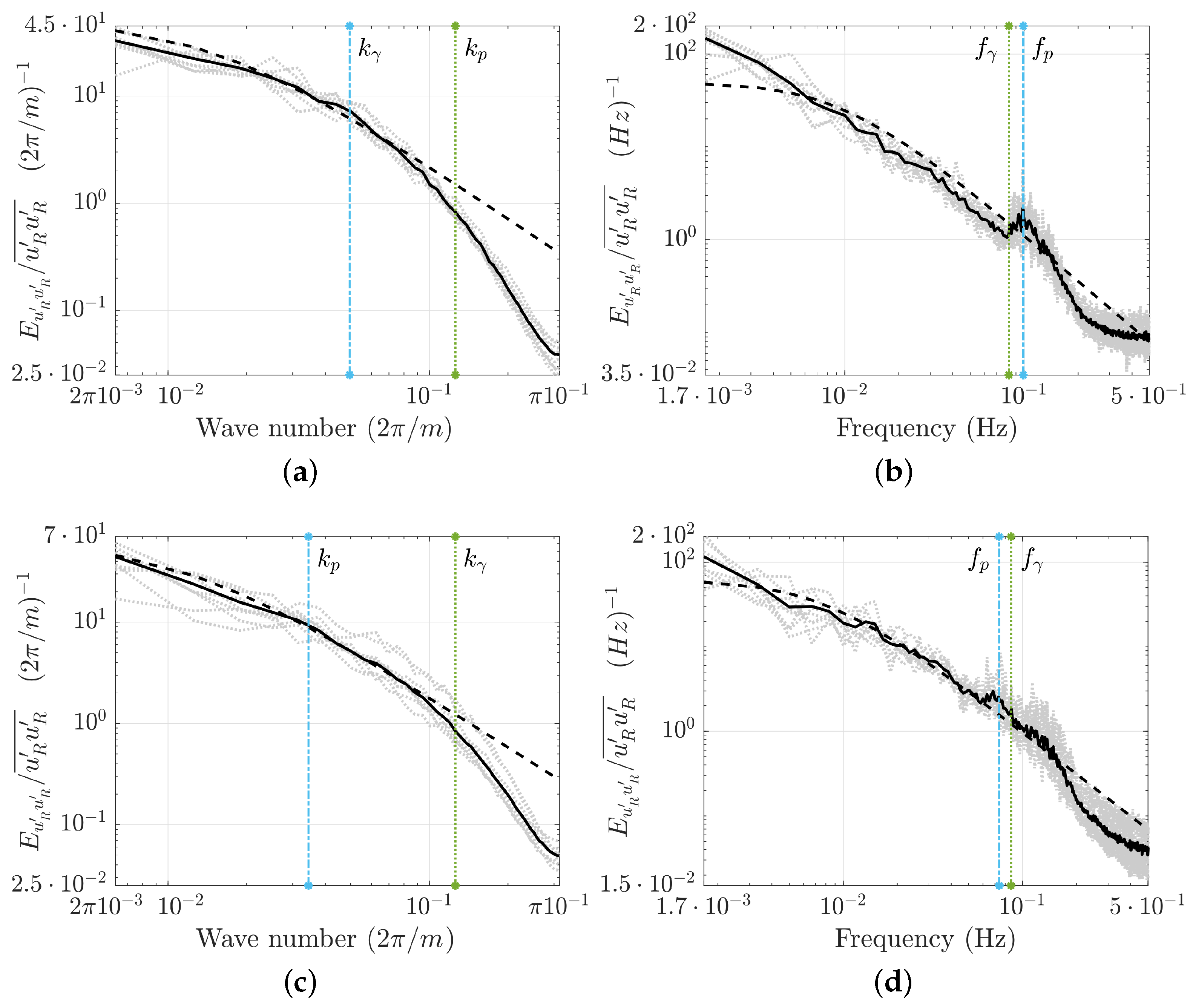
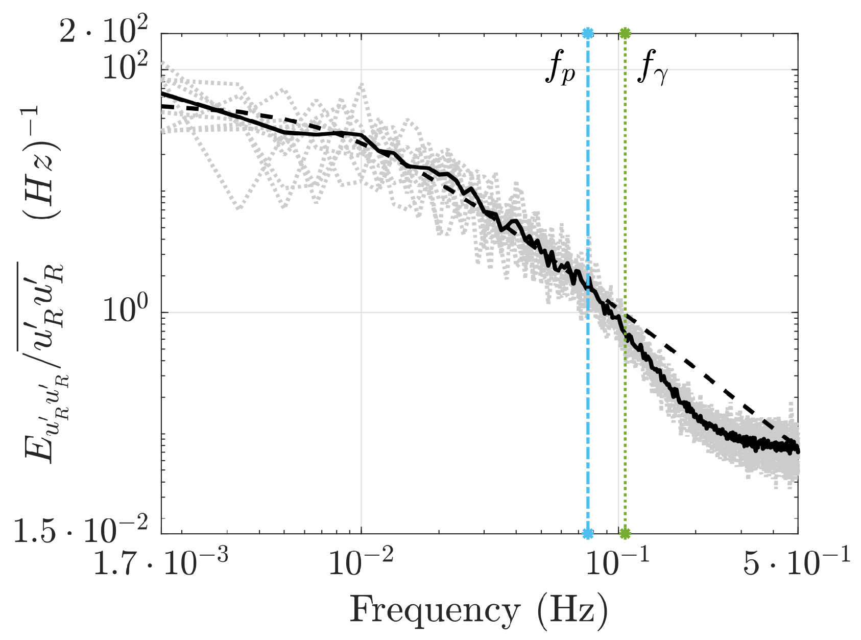
4.2. One-Dimensional Turbulent Spectra

In order to characterize the spectral transfer from the sea-state to the wind, the energy distribution of the RWS fluctuations was analyzed in either space or time dimensions by 1D wave-number (k) or frequency (f) EDF (turbulent spectra). Figure 5 shows, in light grey, for Case 01 (Figure 5a,b) and Case 02a (Figure 5c,d), k- and f-dependent spectra for each 10-min record constituting the 3-h period of each test case. The 3-h ensemble averaged spectrum is depicted by a solid black line.
A reference spectrum taken from the Engineering Sciences Data Unit (ESDU) [73], is plotted in Figure 5 as a dashed black line with the parameters U R , observed integral length scale ( L l = π E k ( 0 ) / [ 2 R k ( 0 ) ] , obtained from E k ), altitude 18 m, and a boundary layer height estimated at 1 km. The ESDU spectrum is defined in the frequency domain, so Taylor’s hypothesis is assumed ( k = w / U R ; E ( k ) = E ( w ) U R ) to obtain the reference k spectra depicted in Figure 5a,c. At large scales, the measured spectra are observed in good agreement with the reference through a region of constant slope, i.e., −5/3 through the inertial sub-range, which is reproduced exactly in the reference spectrum.
At smaller scales, i.e., k (in m s 1 ) and f (in Hz) larger than 10 1 , the observations deviate from the reference, notably as a consequence of the sLiDAR volume filtering (c.f. [58]). The spatial filtering characteristic length scale is represented as being twice the gate length of the sLiDAR ( 2 L γ = 50 m), so the corresponding wave-number scale is k γ = 2 π / ( 2 L γ ) . The sLiDAR filter frequency scale is f γ = U R / ( 2 L γ ) , here estimated from Taylor’s hypothesis with U R = 4.12 m s 1 and U R = 4.29 m s 1 , for Cases 01 and 02a, respectively.
The filter scales k γ and f γ are reported in Figure 5 as vertical green dotted lines. The peak wave-number of the sea-state k p = 2 π / L p and its corresponding frequency f p = 1 / T p (Table 3) are depicted as vertical blue dot-dashed lines in the same figure.
In the f-dependent spectra of Figure 5b,d, f p lies close to f γ . However, a clear peak is observed in the vicinity of f p , denoting an energy transfer from the waves to the wind. The peak present in Case 02a (Figure 5d) is less pronounced than that in Case 01 (Figure 5b), but is still detectable, and the energy does not drop, as was expected from the spatial filtering for f > f γ .
On the contrary, WI disturbances cannot be detected in the wave-number-dependent spectra, and only the spatial filtering effect is visible in Figure 5a,c. These remarks are explained in the next section, looking at the 2D wave-number–angular-frequency spectra.

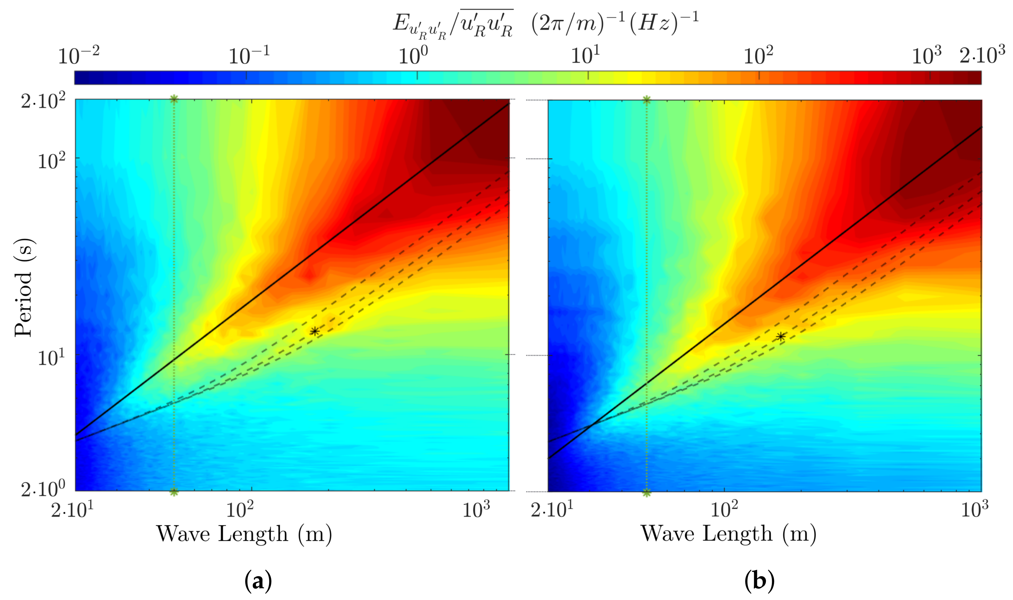
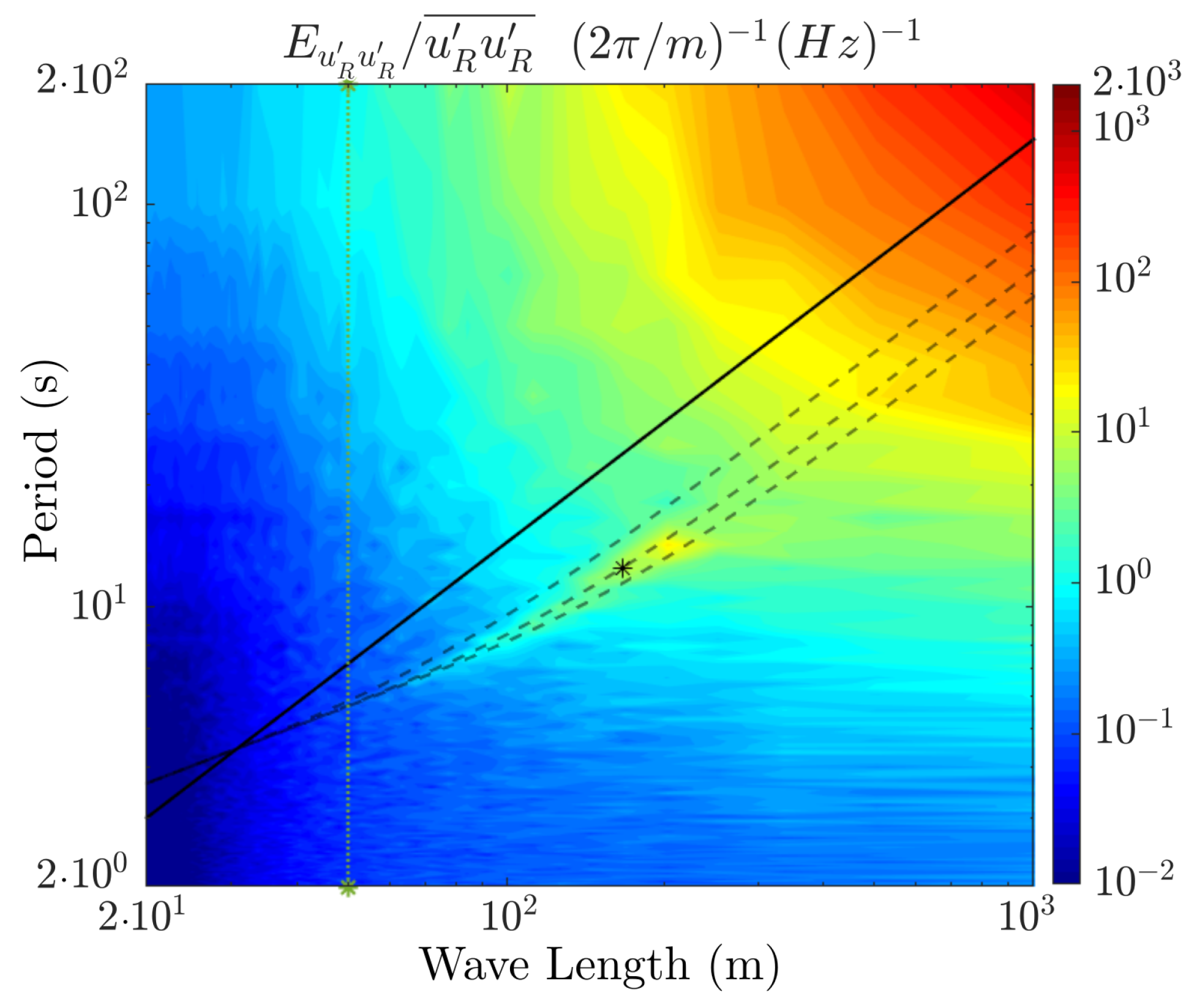
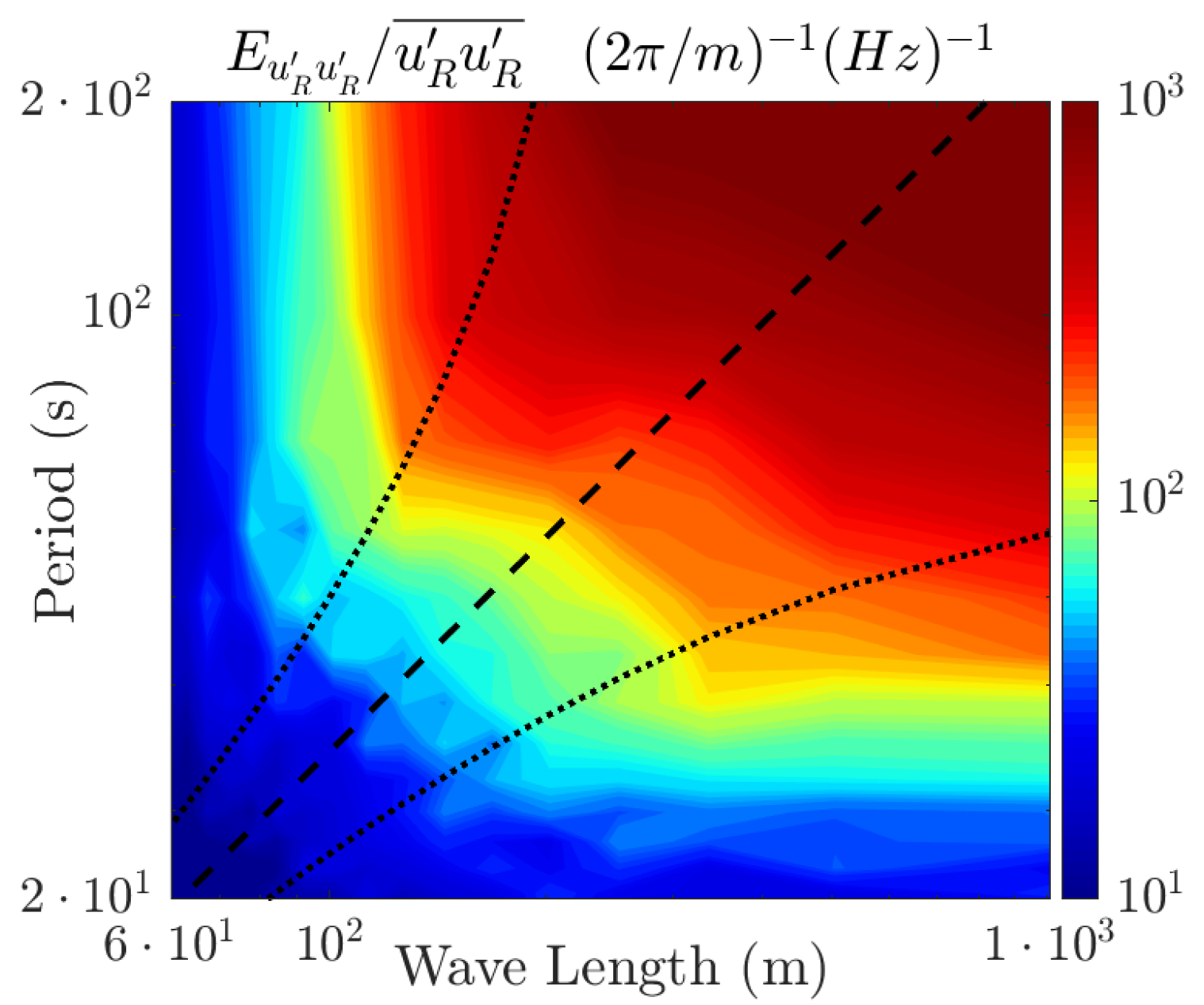
4.3. Two-Dimensional Turbulent Spectrum

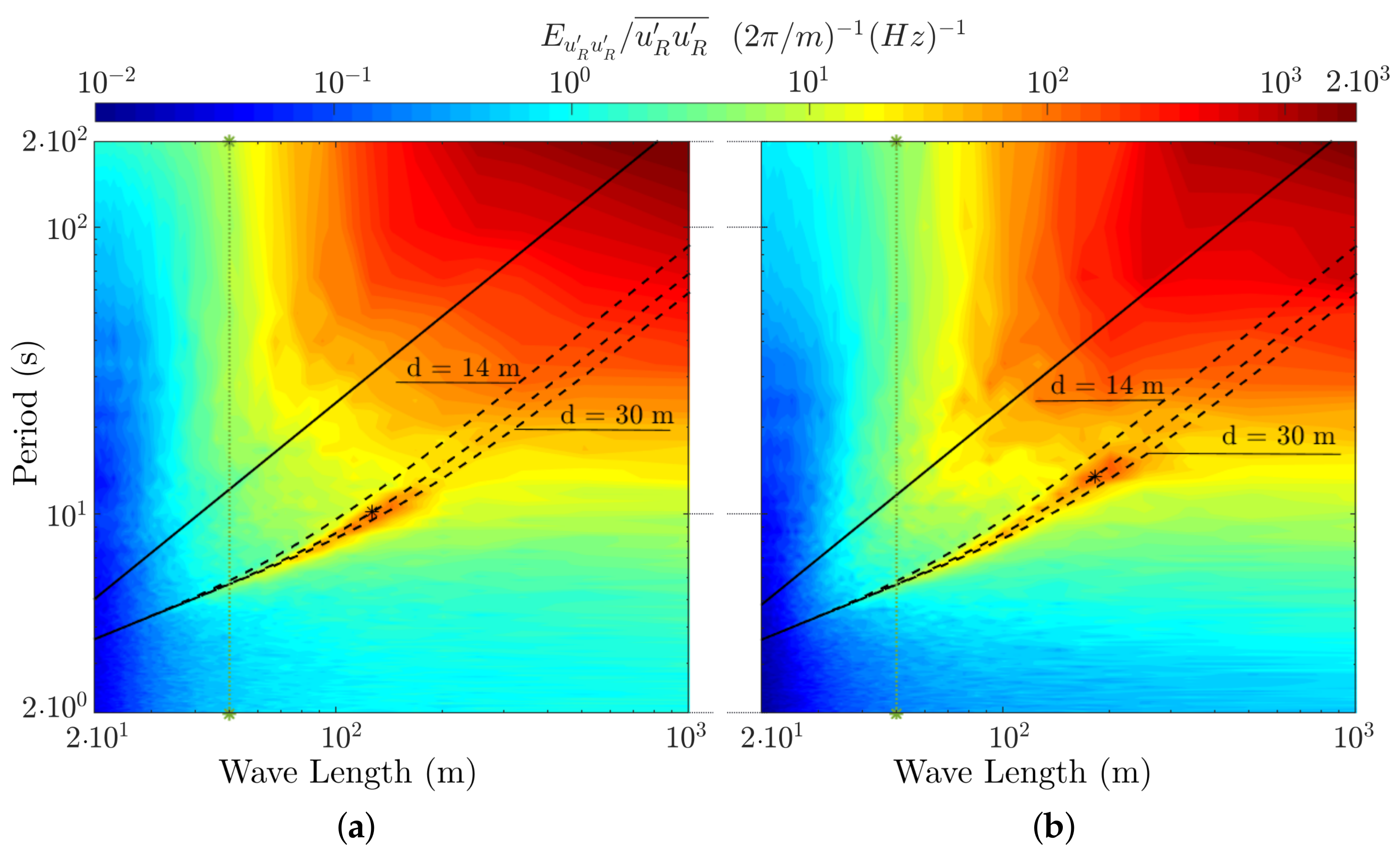
4.3.1. Resultant Single-Sided Spectrum

The sLiDAR in the proposed configuration allows for an original 2D spectral analysis, which is seldom possible in the field. Figure 6 presents the 2D spectra of the RWS E u R u R ( k , w ) , plotted as a function of wave length L = 2 π / k and period T = 2 π / w , for Cases 01 and 02a, in subfigures a and b, respectively. The sea-state peak scale [ T p , L p ] (from WWIII in Table 3) is marked as a black star. The characteristic space filtering discussed in Section 4.2 still applies, such as to mitigate the small-scale fluctuations. The characteristic filter length 2 L γ is therefore reported in the 2D spectra as a green dashed vertical line.
To guide the analysis, different characteristic velocities L / T are plotted with the 2D spectra of Figure 6. According to Taylor’s hypothesis the atmospheric turbulence is convected by U R , here denoted by the black, full line. As expected from a shear-layer flow (c.f. [40]), most of the energy is present for long periods/lengths, with significant spreading around the mean velocity.
Aside from that, and much more relevant here, the 2D spectra of Figure 6 clearly show a second, elongated region of high energy, disconnected from Taylor’s hypothesis. This region includes [ T p , L p ], and precisely follows the three dashed curves denoting c ( k ) , so determined from the dispersion equation.
The dispersion equation is shown in Figure 6 for three different water depths, roughly representing the uncertainty with d = [ 14 , 22 , 30 ] m. As presented earlier, the first two depths correspond to the MSL in the sLiDAR f-LOS. Because WI disturbances are generated at water depths somewhat larger than in the f-LOS, the curve d 30 m is given as an additional reference to the figure. Case 02a (Figure 6b) agrees well with d = 22 ± 8 m. However, as the wind blows from the sea, and the fetch is quite large in Case 01 (Figure 6a), wind is mostly affected by waves from greater water depths than in the f-LOS. Indeed, the WI signature observed in Case 01 suggests the influence of waves propagating at greater depths than those of Case 02a.
In Section 4.2, the wave signature is only observable in the 1D frequency-dependent spectra, where much of its energy is still hidden beneath the predominant atmospheric turbulence, so that it is difficult to dissociate one from the other. On the contrary, in the 2D spectra of Figure 6, the upward transfer of motions from the waves to the wind is evident and easily distinguishable from the atmospheric turbulence.
The impossibility of distinguishing the WI signature in the 1D-spatial spectra (Figure 5a,c) results from its coincidence with a considerable amount of energy in the undisturbed atmosphere, meaning that both systems present a considerable amount of energy at similar length scales ( L p ). Due to the different convection velocities between atmospheric and WI motions, the wave signature arises in the 1D-temporal spectra (Figure 5b,d), as the turbulent content decreases in T p compared to L p .
In Case 02a, T p is higher, and the signature moves towards the atmospheric scales in the space–time domain (Figure 6b). Consequently, the coincidence increases in the 1D frequency-dependent spectrum, leading to the less pronounced peak in Figure 5d compared to Figure 5b.
The sLiDAR spatial filtering also plays an important role in determining the coincidence between the 1D modal distributions of atmospheric turbulence and WI motions. For instance, the atmospheric turbulence at T p is largely filtered by the sLiDAR, since, following Taylor’s hypothesis, U R T p approaches (Case 02a) or falls below (Case 01) the filter scale 2 L γ . On the other hand, L p 2 L γ , so the WI energy content at T p is less filtered. Hence, the sLiDAR filter effect magnifies the relative importance of WI motions in the 1D frequency-dependent spectrum.
As can be seen, the 1D spectra previously discussed give only a partial picture of the modal distribution of turbulent fluctuations. The prominence of the wave signature in the 1D spectra is very sensitive to the coincidence in the 1D scale-dependent modal energy distribution of both the WI and atmospheric turbulence systems. As such, 1D spectral analyses may be unsuitable for an objective evaluation of the WI flow. In the 2D spectra, however, as long as U R and c p are sufficiently far apart with c p U R , the 2D scale-dependent coincidence between atmospheric and WI motions is mitigated, so the two systems can be clearly distinguished from each other in the kw domain. The discussion in Section 5.2 relates these observations about the spectral coincidence of different signals to a qualitative evaluation of their coherence and, consequently, to the possible amount of correlation between them.
The single-quadrant 2D spectra discussed above are more precisely E u R u R ( k , w ) = 2 ( Q + + + Q + ) defined in Equation (6). These are the resultant auto-spectra which, when integrated, lead to the 1D spectra previously observed in Section 4.2.

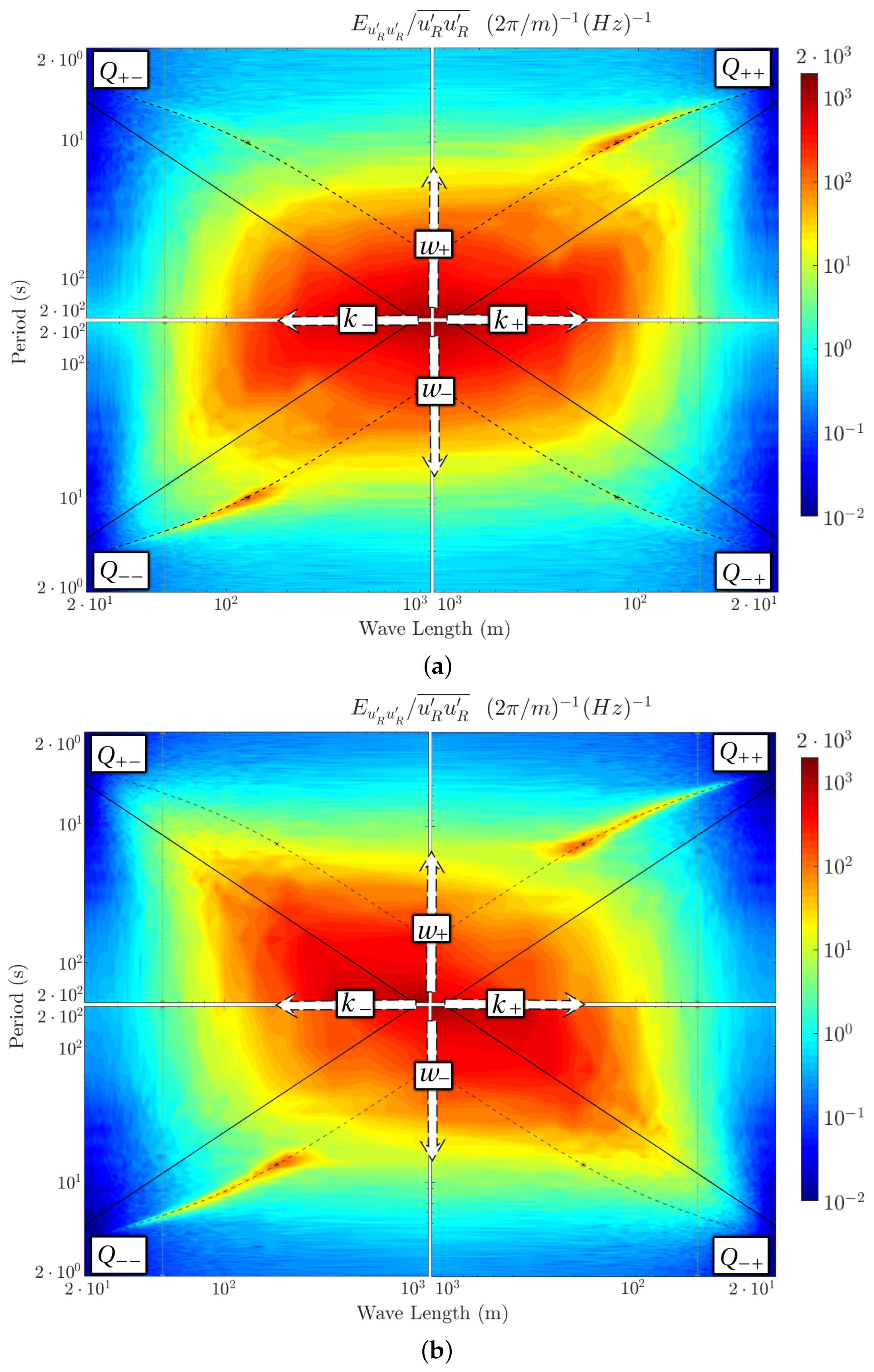
4.3.2. Opposing Directions and the Four-Quadrant Spectrum

As seen the 2D spectrum is defined in four-quadrants Q ± ± , normally referred to by negative and positive wave-numbers k ± or frequencies w ± as in Equation (6). The different quadrants indicate the components that, propagating in different directions, interfere to give the resultant spectrum E u R u R ( k , w ) = 2 ( Q + + + Q + ) previously presented in Figure 6. The four-quadrant spectra of Cases 01 and 02a are given in Figure 7.
The decomposition between signals propagating in opposite directions is particularly useful in Case 02a, as demonstrated in Figure 7b. No WI disturbance is observed for motions traveling from the land to the ocean in quadrant Q + (and Q + ), as they are fully captured traveling in the opposite direction, in Q + + (and Q ). From the ocean to the land, the atmospheric turbulence is limited to very large scales, so the WI disturbances appear in a detached region, even more clearly than in the resultant spectrum that is depicted in Figure 6b.
Note that non-observable WI disturbances may be present at motions traveling from the land to the ocean, either due to wind–wave interactions, or due to the wave reflection at the coast. The fact that they are not seen in Q + in the spectrum shown in Figure 7b indicates that WI disturbances are probably negligible compared to the prevailing atmospheric contribution, but not necessarily absent. In Case 01, (Figure 7a), a slight, rather indistinct wave signature can be observed as occurring from the land to the ocean in quadrant Q + . The counter-propagating WI disturbance can be observed in Case 01 because this is also the counter-propagating WD, where the atmospheric turbulence is weak and mostly restricted to very large scales.

4.4. Rising Wind and Diminishing Sea-State

During the 28 h following Case 02a, meteocean conditions registered a rising wind in an approximately constant direction, while the swell decayed as the significant height and the peak period diminished (Figure 3). Cases 02b and 02c (WA = [ 2.53 , 1.92 ] ) are presented to observe the decay in WI motions during this period in comparison to Case 02a (WA = 3.14 ).
In a first attempt to observe the wave signature, Figure 8 and Figure 9 refer to Case 02b, and can be compared with Case 02a from Figure 4b and Figure 5d. Recall that, for Case 02a, the space–time mapping of the RWS in Figure 4b depicted atmospheric streaks hashed by the wave signature. Similarly in Figure 5d, Case 02a, the WI signature becomes clear, enhancing the modal distribution of energy around the wave peak frequency.
As in Case 02a, the RWS contours of Case 02b in Figure 8 reveal streaks that correlate well with the mean RWS value, and the frequency spectrum of Figure 9 agrees well with the ESDU reference, except for the filtering effect at high frequencies. The wave signature, however, vanished from Case 02b in Figure 8, where atmospheric streaks are elongated and uncorrelated to the wave phase speed, and from Figure 9, that does not reveal any wave-related anomaly in the frequency-dependent spectrum.
If one considers instead the kw spectra from Figure 10 (Cases 02[b–c]), compared with Case 02a, given in Figure 6b, the wave signature is once again observable. It diminishes, and although it is still distinguishable in Case 02b (WA = −2.53 in Figure 10a), it can no longer be clearly discerned in Case 02c (WA = −1.92 in Figure 10b). The 2D spectra shown for Cases 02[b,c] agree well with the expected random sweeping behavior described in [40].
As in Case 02a, Cases 02b and 02c also consider wind and waves traveling in opposite directions, and using the four-quadrant 2D spectra, the resultant spectra can be decomposed, as previously exemplified in Figure 7. Again, the WI flow is observed traveling from the ocean to the land, so that is the component depicted in the 2D spectrum of Figure 11 for Case 02c. Thanks to the opposing directions, the WI disturbance, although weak, is still distinguishable at the lowest WA of Case 02c.
As the WA decreases and the signature diminishes, the principal wave disturbance occurs at scales greater than the wave peak, i.e., [ L p , T p ] from Table 2, indicated by the dots in Figure 10 and Figure 11. This is an indication of the scale-dependent energy transfer occurring between ocean waves and turbulent fluctuations, which favors the propagation of long waves across the WBL.

5. Discussion

5.1. Deviations from the Taylor and Random Sweeping Hypotheses

The contour slopes in the RWS space–time mappings of Figure 4 generally correspond to the atmospheric and WI characteristic velocities, given, respectively, by Taylor’s hypothesis and the wave dispersion equation. The clear exception concerning Taylor’s hypothesis occurs for Case 01 in Figure 4a, where the atmospheric turbulence appears to propagate at lower velocities than the mean RWS.
A clue is given by the discussion on the validity of Taylor’s hypothesis in the lower part of the ABL carried out in [46], where the authors associate an apparent slowdown of turbulent eddies to their increased distortion and the consequent reduction in their life-time. An increasing distortion influences the life-cycle of coherent turbulent structures (c.f. [72,74]), and ultimately gives the impression of turbulent eddies propagating with lower convection velocities in Figure 4a.
Taylor’s hypothesis is here evaluated in view of the 2D spectra of Figure 6, where there is no deviation in the expectancy of the EDF with respect to Taylor’s hypothesis, so that the overall expected convection velocity for the atmospheric turbulence is still the mean RWS. However, a spectral gap disturbance is particularly evident in Case 01, presented in Figure 6a, and adapted (axes and color ranges) as Figure 12. The Figure highlights a region of decreased energy (valley), following Taylor’s hypothesis along the dashed line, and symmetrically apart from that, two regions of increased energy (ridges) denoted by dotted lines. This phenomenon is faintly observable for Case 02a in Figure 6b, but not for Cases 02[b,c] in Figure 10.
The spectral gap described is not predicted by the Random Sweeping hypothesis on which current state-of-the-art kw spectrum models are based [40]. Contrasting with the elliptical contours expected in these models and observed in Cases 02[b,c] in Figure 10, the observance of a bi-modal distribution of the EDF around Taylor’s prediction indicates that the turbulence convection velocity is often slower or faster than the expectancy. This could be due to the periodic mixing of the flow, from either below or above the measurement height. As in [46], Taylor’s hypothesis still provides a good approximation of the expected modal distribution of energy, but fails because turbulence is not frozen.
We cannot identify any measurement-induced bias capable of imposing the features described here on the RWS mappings or the 2D spectra. These deviations from theory are thus assumed to be physical, as, e.g., transient and periodic distortions to the RWS fluctuations are plausible candidates to explain the observations. Recall that, in Figure 4a, the atmospheric streaks are distorted due to WI disturbances in the RWS fluctuations. In Case 01, wind and waves were aligned in a large fetch open to the ocean, so wind–wave interactions were closer to a dynamic equilibrium. Another possibly significant peculiarity of Case 01 is that it is in a stable stratification regime, in which turbulence intermittence (transience and periodicity) is favored by buoyancy effects [75].

5.2. Coherence and Correlation in a Space–Time Perspective

To avoid ambiguity, the term spectral coherence is here employed to qualify the coincidence of two spectral distributions. The term seems appropriate because, provided that two signals are phase-locked to each other, such a similarity is proportional to their magnitude-squared coherence, so evaluating the possibility of second-order correlation between them. Holding their energy at the same scale is a necessary, but not sufficient, condition for correlation. The exact amount of correlation is proportional to the real part of the complex-valued coherence, and thus depends on the exact phase shift between the signals.
The discussion that follows assumes that the total fluctuations u R = u ^ R + u ˜ R are decomposed into atmospheric turbulence ( u ^ R ) and WI motions ( u ˜ R ). This WI decomposition is usually achieved by a wave-coherent (WC) filter [7,21,76]. Due to their importance and for the sake of brevity, WC and WI decompositions will be properly investigated in future works. The present discussion instead, is based on the qualitative inference of the WI flow structure, from the features characterizing the WI signature observed in the 2D spectra of Section 4.3. These 2D spectra reveal that atmospheric and WI motions correlate differently (in terms of spectral coherence) in space and/or time domains, explaining the observations previously evaluated in the 1D spectra of Section 4.2.
For instance, the impossibility of seeing the wave signature in the 1D-spatial spectra (Figure 5a,c) results from the strong coherence between u ^ R and u ˜ R in space ( L p scales). The signature arises in the 1D-temporal spectra (Figure 5b,d) as the coherence decreases in T p compared to L p . In Case 02a, T p is higher, the wave signature moves towards the atmospheric scales in the space–time domain (Figure 6b), and the coherence increases in 1D-temporal spectra, leading to the less pronounced peak in Case 02a (Figure 5d) compared to Case 01 (Figure 5b). Motions that, in one dimension, appear to correlate with u ˜ R in L p or T p , do not correlate with u ˜ R in the space–time domain unless they propagate with velocity c p = L p / T p .
Assuming uncorrelated motions in time or space, the Navier–Stokes equations for u are uncoupled (or weakly coupled through the mean flow) in u ^ and u ˜ (c.f. [7,21]), but this simplification cannot explain some of the features observed in the 2D spectra. Atmospheric and WI motions coexist at the same scales, and so may strongly correlate in either space or time domains if the computation of the cross-correlation functions, or the averaging of governing equations, are exclusively performed in one dimension.
In the combined space–time perspective, however, the correlation is limited as long as | WA | 1, such that Taylor’s convection velocity and the wave peak velocity are sufficiently far apart from each other. With limited correlation, the wave signature is highlighted in the space–time spectra, and the decomposition of uncorrelated atmospheric turbulence and WI motions could be more consistently defined as two different dynamic systems that non-linearly interact with each other. From a mathematical or experimental perspective, this introduces considerable complexity to the decomposition, as the Navier–Stokes equations need to be averaged, or the measurements need to be taken, in space and time domains, simultaneously.
The decomposition between fluctuations traveling in opposite directions is available from the four-quadrant spectra, as demonstrated in Figure 7. Because traveling in the same directions (in the same quadrant of the 2D spectra) is also a requirement for correlation, the spectral coherence discussed here explains why wind–wave interactions (through second-order correlations) are expected to be less significant in wind-opposing wave scenarios.
In decreasing |WA| conditions (Section 4.4), the WI disturbances vanish from the RWS contours and from the 1D frequency spectra. However, with limited coherence to the atmospheric turbulence in the space–time perspective, the signature is still noticeable in the 2D spectrum, which is clearly a more sensitive tool to detect WI disturbances in old seas. The 2D spectrum is so sensitive that it was hard to find measurements without any WI disturbance during the measurement campaign (October 2020 to January 2021, high waves season on the coast of Le Croisic, France).

6. Conclusions

A space–time radial wind speed (RWS) field, registered 18 m above the ocean by the sLiDAR employed on the coast at Le Croisic, was exploited to identify wave-induced (WI) disturbances in the wave boundary layer. In swell-dominated scenarios, the disturbances can be qualitatively evaluated in the RWS space–time contours, as the atmospheric streaks are distorted in velocities and periods corresponding to the wave dynamics. The 1D k- or f-dependent turbulent spectra allow for a partial but quantitative evaluation of these WI disturbances. From this perspective, the wave signature only emerges in the frequency domain, with the WI spectral contribution becoming prominent in the 1D f-dependent spectra. The spectral transfer between sea-state and atmospheric motions is observed, as previously, but not often, reported in the literature.
Unlike the 1D spectra that were previously observed in the literature and in the present study, where the wave signature is either too weak or merged into the turbulent cascade, the wave signature becomes clearly distinguishable from the atmospheric content in the 2D spectra presented here. One reason for the many failed attempts to detect WI disturbances in 1D turbulent spectra may be the partial picture they provide of the energy modal distribution, as a projection of the space–time-dependent energy content in either k or f domains.
The WI signature remains clear in the 2D spectra as long as the waves travel sufficiently faster than the mean wind velocity ( | WA | 1). Compared to 1D spectra, 2D space–time spectrum analysis is, therefore, a more sensitive tool for the detection of WI disturbances in old-sea conditions. These 2D spectra are the first to be measured in an offshore environment at these micro-scales, leading to original and detailed experimental evidence of the full sea-state spectra transferring upwards into the lower part of the ABL.
This original analysis represents a major breakthrough to access the dynamics of micro-scale wind–wave interactions. As this leads to the detailed, simultaneous characterization of the WI flow in both space and time domains, one can then interpret multiple features, which are usually observable but as yet unexplained in the most commonly exploited 1D spectra. For instance, the reason why WI motions preferably appear in the frequency-dependent, rather than in the wave-number-dependent spectra, becomes clear: because the atmospheric turbulence energy content is limited in the wave-predominant periods, but is significant in the wave-predominant lengths.
The new perspectives presented raise a number of questions that will be addressed in future works. Even in flat-bottom cases, these 2D spectra are not exploited as much as 1D spectra in the literature. For this reason, one encounters unexpected features in the modal distribution of the atmospheric turbulence depicted here, such as deviations from the Taylor and Random Sweeping hypotheses. Therefore, we aim to further extend the analyses to canonical and in-land applications.
The lack of other instruments that can measure the space–time mapping of the RWS at similar scales prevents the proper evaluation of the sLiDAR-filtering effect in the 2D spectral domain. The qualitative descriptions of the sLiDAR-filtering effect presented here need to be further refined by numerical evaluations, which will be reported in forthcoming publications.
As has been discussed here, in old-sea conditions, the possibility of correlation between atmospheric and WI motions is limited in the 2D perspective if compared to the 1D alternatives. Consequently, atmospheric and WI motions are more easily identified, and more consistently defined, as different dynamic systems weakly interacting with one another. It is expected that the increasing amount of information revealed by these 2D analyses will drive the development of more accurate WI decompositions.

Author Contributions

Conceptualization, L.P., B.C., Y.P. and S.A.; operation, meteocean monitor and hind-cast, L.P., B.C. and Y.P.; data curation, treatment and analysis, L.P. and B.C.; funding acquisition and project administration, S.A.; supervision, B.C., Y.P. and S.A.; writing—original draft, L.P.; writing—review and editing, L.P., B.C., Y.P. and S.A. All authors have read and agreed to the published version of the manuscript.

Funding

This work is carried out within the framework of the WEAMEC, West Atlantic Marine Energy Community, and with funding from the Pays de la Loire Region. This work was developed in the context of a PhD thesis, funded by research grants from the French Ministry of Research and Higher Education and École Centrale de Nantes.

Data Availability Statement

The data presented in this study are available on request from the corresponding author.

Acknowledgments

We acknowledge the reviewers and the academic editor, for their careful reading and insightful suggestions that have significantly contributed to improving our manuscript.

Conflicts of Interest

The authors declare no conflict of interest. The funders had no role in the design of the study; in the collection, analyses, or interpretation of data; in the writing of the manuscript, or in the decision to publish the results.

Abbreviations

The following abbreviations are used in this manuscript:
1DOne-dimensional
2DTwo-dimensional
ABLAtmospheric Boundary Layer
CNRCarrier-to-noise-ratio
EDFEnergy Density Function
ESDUEngineering Sciences Data Unit
f-LOSfixed LOS
FTFourier Transform
FFTFast FT
LiDARLight Detection and Ranging System
LHEEALaboratory in Hydrodynamics, Energetics and Atmospheric Environment
LOSLine of Sight
MABLMarine ABL
MSLMean Sea Level
PPIPlan Position Indicator
RWSRadial Wind Speed
sLiDARscanning LiDAR
SSTSea Surface Temperature
TITurbulence Intensity
TKETurbulent Kinetic Energy
UTCUniversal Time Coordinated
WAWave Age
WBLWave Boundary Layer
WCWave-Coherent
WDWind Direction
WIWave-Induced
WSWind Speed
WWIIIWAVEWATCH III

Appendix A. Data Quality and Filter

Two methods of identifying poor-quality data are discussed: (i) a fixed Carrier-to-Noise-Ratio (CNR) threshold in Appendix A.1; (ii) RWS spike detection in Appendix A.2. Bad-quality data were first removed from the dataset, and then reconstructed according to Appendix A.3, so that the RWS can be assessed in a uniform space–time grid, as is required for the spectral analyses defined in Section 3.1.

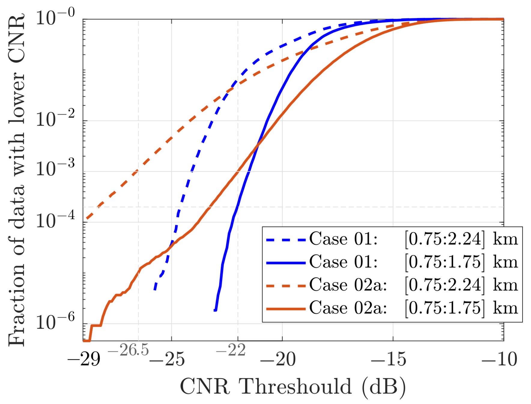
Appendix A.1. Carrier-To-Noise Ratio

The CNR evaluates the back-scattering intensity with respect to noise, so that the higher its value, the better the data quality [68]. A fixed CNR value threshold, below which data are discarded to ensure high-quality datasets, is usually employed in the literature, with values ranging between −22 dB and −29 dB [69]. However, this is shown to induce CNR-dependent statistical properties [69], and is a severe criterion in specific environmental conditions, where the CNR naturally tends towards lower values [70].
The fraction of data filtered as a function of the threshold are shown as cumulative distributions, for Cases 01 and 02a in Figure A1. The cumulative distributions shift towards lower thresholds in Case 02a, and lower CNR values occur more often in more distant measurements. A higher data quality is thus achieved, limiting the total sLiDAR f-LOS ranges (dashed lines in Figure A1) that were exploited from the first 1 km distance (101 gates) closest to the sLiDAR (full lines in Figure A1).
Figure A1. Cumulative distributions of Carrier-to-Noise-Ratio (CNR) occurrences below the threshold. Cases 01 and 02a depicted with full or limited f-LOS range.
Remotesensing 14 03007 g0a1
With the limited 1-km LOS extent, the mean RWS and TI were found to be independent of CNR thresholds lower than −22 dB. However, the independence of these integral variables does not imply the independence of other statistical and more sensitive quantities, such as the turbulent spectra. Referring to the cumulative distributions, a −22 dB threshold discards 0.02% of the data in Case 01 and 0.1% in Case 02a, which is too much for the current objectives, which employ highly detailed Fast Fourier Transforms (FFT).
To perform an FFT, the dataset must be uniformly distributed, so data removal implies data reconstruction, which is scarcely more trustworthy than actual measurements. Note that the quality of the 2D spectra deteriorates completely with the removal of ∼0.1% of the dataset, i.e., a CNR threshold of −26.5 dB if the full LOS range were considered in Case 02a, according to the cumulative distribution of Figure A1. To avoid CNR-dependent biases in future results, the lower threshold of −29 dB was adopted, together with the dataset reduction to a 1 km span, with no data being discarded in Case 01 and a single datapoint in Case 02a.

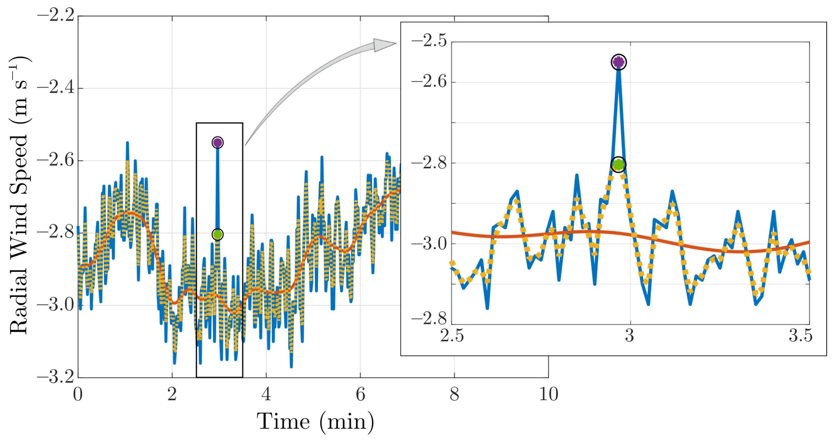
Appendix A.2. Spike Detection and Removal

A spike is defined as data for which the difference between the measurements and their estimate exceeds a certain threshold, which is large enough to be considered non-turbulence-related. Spike detection methods cover the mathematical description of the estimate and the definition of a criterion, and vary in the literature, as their performance is intrinsically flow-dependent [71]. Here, the estimate is given by the low-pass filtered signal, and the threshold is imposed with respect to the difference between the measurement and its estimate. The filter standard deviation and the criterion thresholds are tuned through a graphical inspection of Cases 01 and 02a to filter non-physical outliers.
The spikes are identified in the time domain as the short acquisition sampling period captures RWS fluctuations at smaller scales than the comparatively larger gate spacing. At each gate, there are N time steps t n in a 10-min time series. The low-pass time-filtered signal u α ( x , t ) represents the large-scale motions of the space–time-dependent measurements u ( x , t ) , and is evaluated at a given position x, so the space dependency is omitted below. A single parameter gaussian filter defined in Equation (A1) is applied, where the standard deviation σ α is tuned to 10 s.
u α ( t ) = n = 1 N u ( t n ) · W α ( t n t ) n = 1 N W α ( t n t ) , with W α ( t n t ) = 1 2 π σ α exp ( t n t ) 2 2 σ α 2 .
This method is an alternative to more simplistic approaches, where | u u ¯ | < m σ · σ u (in which case u ¯ is the estimate), with σ u providing the standard deviation of u ( t ) and m σ a constant. An advantage of the proposed procedure is that the estimate includes low-frequency motions, such that spikes remain defined in high frequencies.
The criterion depends on the time-wise difference d n = u n u α between the time-dependent signal u n ( t ) and its estimate u α ( t ) , in comparison to (i) the Round Mean Square difference RMS d i f f = [ ( d n 2 ) / N ] 0.5 , and (ii) its neighbors: (i) | d n | / RMS d i f f > m σ 1 ; and (ii) d n / d n 1 & d n / d n + 1 > m σ 2 . The constants are tuned to m σ 1 = 5 and m σ 2 = 2 . This procedure identified 5 points ( 0.001 % of all) and 305 points ( 0.01 % of all) as spikes, for Cases 01 and 02a, respectively.
An example is given in Figure A2, where the original signal appears in blue and its low-pass filter (with σ α = 10 s) in orange. The identified spike is shown as a purple dot, having its quality close below the threshold. The yellow line and green dot refer to the signal reconstruction described below.
Figure A2. The full blue line exemplifies a time-series of u R ( x , t ) . For spike detection, the full orange line is the low-frequency estimate u α ( x , t ) . For reconstruction, the yellow dotted line is the high-frequency estimate u β ( x , t ) . The spike value is identified by a purple dot, then replaced by the green dot below.
Remotesensing 14 03007 g0a2

Appendix A.3. Signal Reconstruction

For the subsequent analyses relying on FFT algorithms, it is necessary to reconstruct the previously discarded data, as described in Appendix A.1 and Appendix A.2. The data are substituted by their low-pass filtered (Equation (A1) with α β ) signal, with high pass-bands where the (small) filter duration ( 3 σ β ) initially doubles the acquisition period, i.e., σ β = 2 / 3 · [ 1 , 0.25 ] s for Cases 01 and 02[a–c], respectively. Bad-quality data do not contribute to the summation in Equation (A1).
As a last precaution against badly conditioned data, if required, an adaption of the reconstruction is performed by considering an iterative procedure: The filter standard deviation σ β doubles as long as the weighting function spreads too wide in the removed data. Or more precisely, whenever the gaussian weight ( W β ) in Equation (A1) is ten times larger if integrated with bad-quality data than with good-quality data. This threshold is rarely assessed.

References

  1. Thomson, W. Hydrokinetic Solutions and Observations. Philos. Mag. 1871, 42, 326–378. [Google Scholar] [CrossRef]
  2. Jeffreys, H. On the formation of water waves by wind. Proc. R. Soc. Lond. 1925, 107, 189–206. [Google Scholar]
  3. Miles, J.W. On The Generation Of Surface Waves By Shear Flows, Part I. J. Fluid Mech. 1957, 3, 185–204. [Google Scholar] [CrossRef]
  4. Phillips, O.M. On The Generation Of Waves By Turbulent Wind. J. Fluid Mech. 1957, 2, 417–445. [Google Scholar] [CrossRef]
  5. Belcher, S.E.; Hunt, J.C.R. Turbulent Shear Flow Over Slowly Moving Waves. J. Fluid Mech. 1993, 251, 109–148. [Google Scholar] [CrossRef]
  6. Edson, J.B.; Zappa, C.J.; Ware, J.A.; McGillis, W.R.; Hare, J.E. Scalar flux profile relationships over the open ocean. J. Geophys. Res. Ocean. 2004, 109, C08S09. [Google Scholar] [CrossRef] [Green Version]
  7. Hristov, T. Mechanistic, empirical and numerical perspectives on wind-waves interaction. Procedia IUTAM 2018, 26, 102–111. [Google Scholar] [CrossRef]
  8. Tamura, H.; Drennan, W.M.; Collins, C.O.; Graber, H.C. Turbulent Airflow and Wave-Induced Stress Over the Ocean. Bound.-Layer Meteorol. 2018, 169, 47–66. [Google Scholar] [CrossRef]
  9. Patton, E.G.; Sullivan, P.P.; Kosović, B.; Dudhia, J.; Mahrt, L.; Žagar, M.; Marić, T. On the Influence of Swell Propagation Angle on Surface Drag. J. Appl. Meteorol. Climatol. 2019, 58, 1039–1059. [Google Scholar] [CrossRef] [Green Version]
  10. Porchetta, S.; Temel, O.; Muñoz Esparza, D.; Reuder, J.; Monbaliu, J.; van Beeck, J.; van Lipzig, N. A new roughness length parameterization accounting for wind–wave (mis)alignment. Atmos. Chem. Phys. 2019, 19, 6681–6700. [Google Scholar] [CrossRef] [Green Version]
  11. Sullivan, P.P.; McWilliams, J.C.; Moeng, C.H. Simulation of turbulent flow over idealized water waves. J. Fluid Mech. 2000, 404, 47–85. [Google Scholar] [CrossRef] [Green Version]
  12. Yang, D.; Shen, L. Direct-simulation-based study of turbulent flow over various waving boundaries. J. Fluid Mech. 2010, 650, 131–180. [Google Scholar] [CrossRef] [Green Version]
  13. Yang, D.; Meneveau, C.; Shen, L. Effect of downwind swells on offshore wind energy harvesting—A large-eddy simulation study. Renew. Energy 2014, 70, 11–23. [Google Scholar] [CrossRef]
  14. Sullivan, P.P.; McWilliams, J.C.; Patton, E.G. Large-Eddy Simulation of Marine Atmospheric Boundary Layers above a Spectrum of Moving Waves. J. Atmos. Sci. 2014, 71, 4001–4027. [Google Scholar] [CrossRef] [Green Version]
  15. Hao, X.; Shen, L. Wind-wave coupling study using LES of wind and phase-resolved simulation of nonlinear waves. J. Fluid Mech. 2019, 874, 391–425. [Google Scholar] [CrossRef]
  16. Obukhov, A.M. Turbulence in an Atmosphere with a Non-Uniform Temperature. Bound.-Layer Meteorol. 1946, 2, 7–29. [Google Scholar] [CrossRef]
  17. Monin, A.S.; Obukhov, A.M. Basic Laws of Turbulent Mixing in the Surface Layer of the Atmosphere. Contrib. Geophys. Inst. Acad. Sci. USSR 1954, 24, 163–187. [Google Scholar]
  18. Businger, J.A.; Wyngaard, J.C.; Izumi, Y.; Bradley, E.F. Flux-Profile Relationships in the Atmospheric Surface Layer. J. Atmos. Sci. 1971, 28, 181–189. [Google Scholar] [CrossRef]
  19. Sjöblom, A.; Smedman, A.S. The turbulent kinetic energy budget in the marine atmospheric surface layer. J. Geophys. Res. Ocean. 2002, 107, 6-1–6-18. [Google Scholar] [CrossRef]
  20. Donelan, M.A.; Dobson, F.W.; Smith, S.D.; Anderson, R.J. On the Dependence of Sea Surface Roughness on Wave Development. J. Phys. Oceanogr. 1993, 23, 2143–2149. [Google Scholar] [CrossRef] [Green Version]
  21. Cifuentes-Lorenzen, A.; Edson, J.B.; Zappa, C.J. Air–Sea Interaction in the Southern Ocean: Exploring the Height of the Wave Boundary Layer at the Air–Sea Interface. Bound.-Layer Meteorol. 2018, 169, 461–482. [Google Scholar] [CrossRef]
  22. Hristov, T.; Ruiz-Plancarte, J. Dynamic Balances in a Wavy Boundary Layer. J. Phys. Oceanogr. 2014, 44, 3185–3194. [Google Scholar] [CrossRef]
  23. Pierson, W.J.; Marks, W. The power spectrum analysis of ocean-wave records. Eos Trans. Am. Geophys. Union 1952, 33, 834–844. [Google Scholar] [CrossRef]
  24. Kitaigorodskii, S.A. On the Theory of the Equilibrium Range in the Spectrum of Wind-Generated Gravity Waves. J. Phys. Oceanogr. 1983, 13, 816–827. [Google Scholar] [CrossRef] [Green Version]
  25. Ōkubo, A. Oceanic diffusion diagrams. Deep Sea Res. Oceanogr. Abstr. 1971, 18, 789–802. [Google Scholar] [CrossRef]
  26. Golitsyn, G. Coefficient of Horizontal Eddy Diffusion of a Tracer on the Water Surface as a Function of the Wave Age. Izv. Atmos. Ocean. Phys. 2011, 47, 393–398. [Google Scholar] [CrossRef]
  27. Hristov, T.S.; Miller, S.D.; Friehe, C.A. Dynamical coupling of wind and ocean waves through wave-induced air flow. Nature 2003, 422, 55–58. [Google Scholar] [CrossRef]
  28. Kolmogorov, A. The Local Structure of Turbulence in Incompressible Viscous Fluid for Very Large Reynolds’ Numbers. Akad. Nauk. SSSR Dokl. 1941, 30, 301–305. [Google Scholar]
  29. Harris, D.L. The Wave-Driven Wind. J. Atmos. Sci. 1966, 23, 688–693. [Google Scholar] [CrossRef] [Green Version]
  30. Hanley, K.E.; Belcher, S.E. Wave-Driven Wind Jets in the Marine Atmospheric Boundary Layer. J. Atmos. Sci. 2008, 65, 2646–2660. [Google Scholar] [CrossRef] [Green Version]
  31. Cathelain, M. Development of a Deterministic Numerical Model for the Study of the Coupling between an Atmospheric Flow and a Sea State. Ph.D. Thesis, Ecole Centrale de Nantes (ECN), Nantes, France, 2017. [Google Scholar]
  32. Edson, J.B.; Jampana, V.; Weller, R.A.; Bigorre, S.P.; Plueddemann, A.J.; Fairall, C.W.; Miller, S.D.; Mahrt, L.; Vickers, D.; Hersbach, H. On the Exchange of Momentum over the Open Ocean. J. Phys. Oceanogr. 2013, 43, 1589–1610. [Google Scholar] [CrossRef] [Green Version]
  33. Mastenbroek, C. Wind-Wave Interaction. Ph.D. Thesis, TU Delft, Delft, The Netherlands, 1996. [Google Scholar]
  34. Edson, J.B.; Fairall, C.W. Similarity Relationships in the Marine Atmospheric Surface Layer for Terms in the TKE and Scalar Variance Budgets. J. Atmos. Sci. 1998, 55, 2311–2328. [Google Scholar] [CrossRef]
  35. Yousefi, K.; Veron, F. Boundary layer formulations in orthogonal curvilinear coordinates for flow over wind-generated surface waves. J. Fluid Mech. 2020, 888, A11. [Google Scholar] [CrossRef]
  36. Benilov, A.Y.; Kouznetsov, O.A.; Panin, G.N. On the analysis of wind wave-induced disturbances in the atmospheric turbulent surface layer. Bound.-Layer Meteorol. 1974, 6, 269–285. [Google Scholar] [CrossRef]
  37. Snyder, R.L.; Dobson, F.W.; Elliott, J.A.; Long, R.B. Array measurements of atmospheric pressure fluctuations above surface gravity waves. J. Fluid Mech. 1981, 102, 1–59. [Google Scholar] [CrossRef]
  38. Grare, L.; Lenain, L.; Melville, W.K. Wave-Coherent Airflow and Critical Layers over Ocean Waves. J. Phys. Oceanogr. 2013, 43, 2156–2172. [Google Scholar] [CrossRef]
  39. Taylor, G.I. The Spectrum of Turbulence. Proc. R. Soc. Lond. Ser. A Math. Phys. Sci. 1938, 164, 476–490. [Google Scholar] [CrossRef] [Green Version]
  40. Wilczek, M.; Narita, Y. Wave-number–frequency spectrum for turbulence from a random sweeping hypothesis with mean flow. Phys. Rev. E Stat. Nonlinear Soft Matter Phys. 2012, 86, 066308. [Google Scholar] [CrossRef] [Green Version]
  41. Craik, A.D. The origins of water wave theory. Annu. Rev. Fluid Mech. 2004, 36, 1–28. [Google Scholar] [CrossRef]
  42. Janssen, P. The Interaction of Ocean Waves and Wind; Cambridge University Press: Cambridge, UK, 2004. [Google Scholar]
  43. Desmars, N. Real-Time Reconstruction and Prediction of Ocean Wave Fields from Remote Optical Measurements. Ph.D. Thesis, École Centrale de Nantes, Nantes, France, 2020. [Google Scholar]
  44. Leckler, F.; Ardhuin, F.; Peureux, C.; Benetazzo, A.; Bergamasco, F.; Dulov, V. Analysis and Interpretation of Frequency–Wavenumber Spectra of Young Wind Waves. J. Phys. Oceanogr. 2015, 45, 2484–2496. [Google Scholar] [CrossRef]
  45. Plant, W.J. Short wind waves on the ocean: Wavenumber-frequency spectra. J. Geophys. Res. Ocean. 2015, 120, 2147–2158. [Google Scholar] [CrossRef] [Green Version]
  46. Cheng, Y.; Sayde, C.; Li, Q.; Basara, J.; Selker, J.; Tanner, E.; Gentine, P. Failure of Taylor’s hypothesis in the atmospheric surface layer and its correction for eddy-covariance measurements. Geophys. Res. Lett. 2017, 44, 4287–4295. [Google Scholar] [CrossRef]
  47. Kraichnan, R.H. Kolmogorov’s Hypotheses and Eulerian Turbulence Theory. Phys. Fluids 1964, 7, 1723–1734. [Google Scholar] [CrossRef]
  48. He, G.W.; Zhang, J.B. Elliptic model for space-time correlations in turbulent shear flows. Phys. Rev. E 2006, 73, 055303. [Google Scholar] [CrossRef] [Green Version]
  49. Narita, Y. Spectral moments for the analysis of frequency shift, broadening, and wavevector anisotropy in a turbulent flow. Earth Planets Space 2017, 69, 73–83. [Google Scholar] [CrossRef] [Green Version]
  50. Peña, A.; Mann, J. Turbulence Measurements with Dual-Doppler Scanning Lidars. Remote Sens. 2019, 11, 2444. [Google Scholar] [CrossRef] [Green Version]
  51. Chan, P.W. Generation of an Eddy Dissipation Rate Map at the Hong Kong International Airport Based on Doppler Lidar Data. J. Atmos. Ocean. Technol. 2011, 28, 37–49. [Google Scholar] [CrossRef]
  52. Nijhuis, A.C.P.O.; Thobois, L.P.; Barbaresco, F.; Haan, S.D.; Dolfi-Bouteyre, A.; Kovalev, D.; Krasnov, O.A.; Vanhoenacker-Janvier, D.; Wilson, R.; Yarovoy, A.G. Wind Hazard and Turbulence Monitoring at Airports with Lidar, Radar, and Mode-S Downlinks: The UFO Project. Bull. Am. Meteorol. Soc. 2018, 99, 2275–2293. [Google Scholar] [CrossRef] [Green Version]
  53. Lothon, M.; Lenschow, D.H.; Mayor, S.D. Doppler Lidar Measurements of Vertical Velocity Spectra in the Convective Planetary Boundary Layer. Bound.-Layer Meteorol. 2009, 132, 205–226. [Google Scholar] [CrossRef]
  54. Barlow, J.F.; Dunbar, T.M.; Nemitz, E.G.; Wood, C.R.; Gallagher, M.W.; Davies, F.; O’Connor, E.; Harrison, R.M. Boundary layer dynamics over London, UK, as observed using Doppler lidar during REPARTEE-II. Atmos. Chem. Phys. 2011, 11, 2111–2125. [Google Scholar] [CrossRef] [Green Version]
  55. Smalikho, I.N.; Banakh, V.A.; Pichugina, Y.L.; Brewer, W.A.; Banta, R.M.; Lundquist, J.K.; Kelley, N.D. Lidar Investigation of Atmosphere Effect on a Wind Turbine Wake. J. Atmos. Ocean. Technol. 2013, 30, 2554–2570. [Google Scholar] [CrossRef]
  56. Pichugina, Y.L.; Brewer, W.A.; Banta, R.M.; Choukulkar, A.; Clack, C.T.M.; Marquis, M.C.; McCarty, B.J.; Weickmann, A.M.; Sandberg, S.P.; Marchbanks, R.D.; et al. Properties of the offshore low level jet and rotor layer wind shear as measured by scanning Doppler Lidar. Wind Energy 2017, 20, 987–1002. [Google Scholar] [CrossRef]
  57. Désert, T.; Knapp, G.; Aubrun, S. Quantification and Correction of Wave-Induced Turbulence Intensity Bias for a Floating LIDAR System. Remote Sens. 2021, 13, 2973. [Google Scholar] [CrossRef]
  58. Bastine, D.; Wächter, M.; Peinke, J.; Trabucchi, D.; Kühn, M. Characterizing Wake Turbulence with Staring Lidar Measurements. J. Phys. Conf. Ser. 2015, 625, 012006. [Google Scholar] [CrossRef]
  59. Global Wind Atlas (Version 3.1). Technical University of Denmark (DTU). 2021. Available online: https://globalwindatlas.info (accessed on 29 May 2022).
  60. Shimada, S.; Goit, J.P.; Ohsawa, T.; Kogaki, T.; Nakamura, S. Coastal wind measurements using a single scanning LiDAR. Remote Sens. 2020, 12, 1347. [Google Scholar] [CrossRef] [Green Version]
  61. Stull, R.B. An Introduction to Boundary Layer Meteorology; Cambridge University Press: Cambridge, UK, 1989; p. 177. [Google Scholar]
  62. Spiegel, E.A.; Veronis, G. On the Boussinesq Approximation for a Compressible Fluid. Astrophys. J. 1960, 131, 442. [Google Scholar] [CrossRef]
  63. Sekimoto, A.; Kawahara, G.; Sekiyama, K.; Uhlmann, M.; Pinelli, A. Turbulence- and buoyancy-driven secondary flow in a horizontal square duct heated from below. Phys. Fluids 2011, 23, 075103. [Google Scholar] [CrossRef]
  64. Lazure, P.; Dumas, F. An external–internal mode coupling for a 3D hydrodynamical model for applications at regional scale (MARS). Adv. Water Resour. 2008, 31, 233–250. [Google Scholar] [CrossRef]
  65. Boudière, E.; Maisondieu, C.; Ardhuin, F.; Accensi, M.; Pineau-Guillou, L.; Lepesqueur, J. A suitable metocean hindcast database for the design of Marine energy converters. Int. J. Mar. Energy 2013, 3–4, e40–e52. [Google Scholar] [CrossRef] [Green Version]
  66. Perignon, Y. Assessing accuracy in the estimation of spectral content in wave energy resource on the French Atlantic test site SEMREV. Renew. Energy 2017, 114, 145–153. [Google Scholar] [CrossRef]
  67. Accensi, M.; Alday, M.; Maisondieu, C.; Raillard, N.; Darbynian, D.; Old, C.; Sellar, B.; Thilleul, O.; Perignon, Y.; Payne, G.S.; et al. ResourceCODE framework: A high-resolution wave parameter dataset for the European Shelf and analysis toolbox. In Proceedings of the 14th European Wave and Tidal Energy Conference, Plymouth, UK, 5–9 September 2021; pp. 2182-1–2182-9. [Google Scholar]
  68. Gryning, S.E.; Floors, R.; Peña, A.; Batchvarova, E.; Brümmer, B. Weibull Wind-Speed Distribution Parameters Derived from a Combination of Wind-Lidar and Tall-Mast Measurements Over Land, Coastal and Marine Sites. Bound.-Layer Meteorol. 2016, 159, 329–348. [Google Scholar] [CrossRef] [Green Version]
  69. Gryning, S.E.; Floors, R. Carrier-to-Noise-Threshold Filtering on Off-Shore Wind Lidar Measurements. Sensors 2019, 19, 592. [Google Scholar] [CrossRef] [PubMed] [Green Version]
  70. Beck, H.; Kühn, M. Dynamic Data Filtering of Long-Range Doppler LiDAR Wind Speed Measurements. Remote Sens. 2017, 9, 561. [Google Scholar] [CrossRef] [Green Version]
  71. Suomi, I.; Gryning, S.E.; O’Connor, E.J.; Vihma, T. Methodology for obtaining wind gusts using Doppler lidar. Q. J. R. Meteorol. Soc. 2017, 143, 2061–2072. [Google Scholar] [CrossRef] [Green Version]
  72. Jiménez, J. Coherent structures in wall-bounded turbulence. J. Fluid Mech. 2018, 842, P1. [Google Scholar] [CrossRef] [Green Version]
  73. Engineering Sciences Data Unit. Characteristics of atmospheric turbulence near the ground. Part 2: Single point data for strong winds (neutral atmosphere). In ESDU 85020; Engineering Sciences Data Unit: London, UK, 1985. [Google Scholar]
  74. Yang, D.; Shen, L. Characteristics of coherent vortical structures in turbulent flows over progressive surface waves. Phys. Fluids 2009, 21, 125106. [Google Scholar] [CrossRef]
  75. Nappo, C.J.; Hiscox, A.L.; Miller, D.R. A Note on Turbulence Stationarity and Wind Persistence Within the Stable Planetary Boundary Layer. Bound.-Layer Meteorol. 2010, 136, 165–174. [Google Scholar] [CrossRef]
  76. Paskin, L.; Perignon, Y.; Conan, B.; Aubrun, S. Numerical study on the Wave Boundary Layer, its interaction with turbulence and consequences on the wind energy resource in the offshore environment. J. Phys. Conf. Ser. 2020, 1618, 062046. [Google Scholar] [CrossRef]
Figure 1. The sLiDAR on the balcony of a seafront villa at Le Croisic, France. Radial Line-Of-Sight (R, LOS), and vertical (z) axis. Roll ( ψ ), pitch (elevation angle θ ), and yaw (azimuth angle ϕ ) angular movements.
Remotesensing 14 03007 g001
Figure 2. sLiDAR position denoted by a red dot and water depth displayed by the colormap. (a) Location of Le Croisic on the French west Atlantic coast. The wind rose for Le Croisic was taken from the Global Wind Atlas [59], covering the period 2008–2017. (b) View of Le Croisic peninsula, with the Plan Position Indicator (PPI) scans for WD determination in the black sector, and staring mode measurements’ lines (f-LOS) for Case 01 (blue) and Cases 02[a–c] (red) in dashed lines. Oceanic conditions were estimated from the HOMERE hind-cast database. The hind-cast grid is depicted by its nodes in yellow dots; probing was performed in the node depicted in magenta.
Remotesensing 14 03007 g002
Figure 3. Evolution of wind and sea-state quantities around Cases 01 (left) and 02[a–c] (right). (a,b) Horizontal Wind Speed (WS) and Wind Direction (WD). Wave model (WWIII) hind-cast: (c,d) the significant wave height ( H s ) and peak period ( T p ); (e,f) the wave peak direction ( α w ) and directional spreading ( β w ). Horizontal lines in (a,b,e,f) denote the sLiDAR fLOS-aligned directions ϕ L and ϕ L 180 °. Vertical lines denote the initial, middle and final moments of the selected periods.
Remotesensing 14 03007 g003
Figure 4. 10-min records of the Radial Wind Speed (RWS) from (a) Case 01, and (b) Case 02a. Mean RWS in dash-dotted lines. Peak wave phase and group velocities ( c p and c g ) slopes as dashed and dotted lines, respectively, dashed lines being distant by T p (Table 3). An indicative value of 0.5 RWS is provided for comparison in (a).
Remotesensing 14 03007 g004
Figure 5. (a,c) Wave-number k and (b,d) frequency f dependent 1D turbulent spectra E u R u R ; for (a,b) Case 01, and (c,d) Case 02a. Observed 10-min spectra in light grey, and the 3-h average in black full lines. The Engineering Sciences Data Unit (ESDU) reference is given in black dashed lines. Vertical blue lines stand for the wave peak scales k p and f p , and green lines show the filter scales k γ and f γ , for wave-number and frequency spectra, respectively.
Remotesensing 14 03007 g005
Figure 6. Wave-number–angular-frequency 2D turbulent spectra E u R u R ( k , w ) , for (a) Case 01 and (b) Case 02a. The mean RWS velocity is depicted by a black full line, and the wave velocity as dashed lines for d = [ 14 , 22 , 30 ] m. The wave peak scale ( L p , T p ) is denoted by a star. The sLiDAR filter wave-length is given in the green dashed vertical lines.
Remotesensing 14 03007 g006
Figure 7. Four-quadrants ( Q ± ± ) of the Energy Density Function (EDF) of u R u R , referred to by negative and positive wave-numbers k ± or angular-frequencies w ± . (a) Case 01 with waves and wind aligned in the same direction (Ocean to land) in quadrants Q + + and Q . (b) Case 02a with the wind aligned in the opposite direction (Land to ocean) in quadrants Q + and Q + .
Remotesensing 14 03007 g007
Figure 8. RWS contours for Case 02b. Mean RWS and peak wave phase velocity slopes as dash-dotted and dashed lines, respectively. Dashed lines are at a distance of T p .
Remotesensing 14 03007 g008
Figure 9. 1D frequency dependent spectra for Case 02b. Observations of 10-min spectra in light grey, the 3-h average in black full lines, and the ESDU reference in black dashed lines.
Remotesensing 14 03007 g009
Figure 10. Wave-number–angular-frequency 2D turbulent spectra E u R u R ( k , w ) , for diminishing WA scenarios in (a) Case 02b and (b) Case 02c. The lines denote the characteristic scales described for Case 02a in Figure 6b.
Remotesensing 14 03007 g010
Figure 11. One quadrant ( Q + + ) of the wave-number–angular-frequency 2D turbulent spectrum E u R u R ( k , w ) for Case 02c. The lines denote the characteristic scales described in Figure 6.
Remotesensing 14 03007 g011
Figure 12. Spectral valley (dashed) and ridges (dotted), observed in the 2D turbulent spectra of Case 01 in Figure 6. Here adapted: axes and color ranges.
Remotesensing 14 03007 g012
Table 1. Staring mode scans for Case 01 (f-LOS 01) and Cases 02[a–c] (f-LOS 02); and PPI mode scans for the reconstruction of the wind speed (WS) and wind direction (WD). The elevation angle is θ = 0° and the gate length L γ = 25 m.
Scan ϕ L Rot. SpeedGate SpacingFirst GateLast GateAcc. TimeDuration
(°)(°s 1 )(m)(km)(km)(s)(s)
f-LOS 01221.80101.002.001.00600
f-LOS 02221.80100.751.750.25600
PPI[154–199]3250.501.751.0016
Table 2. Summary of the wind parameters for each test case. Date and time; f-LOS total average radial wind speed (RWS) U R , wind direction (WD), turbulence intensity (TI), air–sea temperature difference Δ T , and the bulk Richardson number R i b .
Case IDDayStart Time U R WDTI Δ T Ri b
(UTC)(m s 1 )(°)(%)(°C)(Stability)
0112 November 202011:10:324.122128.61.40.04 (Stable)
02a4 November 202007:10:244.296010.0−6.2−0.17 (Unstable)
02b4 November 202019:41:195.315113.7−4.6−0.09 (Unstable)
02c5 November 202004:44:306.935612.1−7.2−0.08 (Unstable)
Table 3. Summary of the sea-state parameters for each test case. Wave age (WA); significant height H s , wave peak period T p and length L p , phase and group velocities c p and c g , mean wave direction α w , and directional spreading β w .
Case IDWA H s T p L p c p c g α w β w
(m)(s)(m)(m s 1 )(m s 1 )(°)(°)
013.01.310.112712.59.424126
02a−3.11.013.518113.511.424730
02b−2.50.713.217713.411.324946
02c−1.90.612.516613.311.021971
Publisher’s Note: MDPI stays neutral with regard to jurisdictional claims in published maps and institutional affiliations.

