Effects of Human Activities on Urban Vegetation: Explorative Analysis of Spatial Characteristics and Potential Impact Factors

Abstract

Since the 21st century, large cities around the world have experienced the transition from economically destructive development to a harmonious eco-environment. Understanding the dynamic relationships between human activities and urban eco-environment in this transition is a challenging and essential topic. The normalized difference vegetation index (NDVI) can reflect the urban vegetation cover status well. Socio-economic indexes can present the intensity and spatiality of human activities quantitatively. This work aims to use traditional regression models and machine learning algorithms to analyze the impact of socio-economic factors on NDVI accurately. Random forest regression (RFR) was performed to initially assess the contributions of all factors on NDVI, which was the numerical basis for feature selection. Subsequently, detailed dynamic relationship simulations were implemented using geographically weighted regression. In the case of Wuhan in China, the results showed that the goodness-of-fit of NDVI with socio-economic factors generally exceeded 50%. The influence coefficients changed from negative to positive, and 2010 was the turning point, indicating that human activities gradually played a favorable role in protecting vegetation during this transition period. The urban–rural interface, which was located between urban centers and marginal urban suburbs, was the area where human activities contributed most to vegetation. Thus, policy makers should focus on planning and managing housing construction and vegetation planting in urban–rural interface to relieve the population burden of the central area and improve the environmental conditions of the urban eco-environment subconsciously.

1. Introduction

Vegetation is the key to carbon and energy exchange between the atmosphere and land surface. The dependence relation between human activity and vegetation change was remarkable in some ecosystems with significant vegetation change [1,2,3], such as the oasis area in arid regions [4] and megacity areas [5,6]. In recent years, rapid urban sprawl and its associated dense population and economic conditions have exerted an increasingly great influence on the eco-environment [2,7], which has changed the bio-physical and chemical characteristics of different land use types [8,9,10], especially for vegetation. At the same time, human activity, such as the series activities of land-use management in China and India, has become the main driver of “Greening Earth” [11]. Therefore, coupling analysis between human activities and vegetation is important to understand their relationship and to develop appropriate management policies [12].

Coupling analysis can be broadly divided into qualitative and quantitative methods. Qualitative methods focus on describing the characteristics and details of the research subject, which can result in a high degree of uncertainty and subjectivity [1,13]. Therefore, many researchers explore numerical methods to quantitatively assess study objects, as well as to further use mathematical models to delve into the dynamic relationships between objects in terms of the degree of influence, inhibitory effects, and facilitative effects.

The normalized difference vegetation index (NDVI) is widely used to quantitatively reflect the vegetation growth condition [14] by the difference between near-infrared (vegetation strongly reflected) and red light (vegetation absorbed) in multispectral remote sensing data [15,16,17]. For example, Wu Zijing et al. evaluated the level of eco-environment in the Greater Bay Area (Guangdong–Hong Kong–Macao) by extracting NDVI annual maximum from multi-temporal remote sensing data [17]. To understand the drivers of vegetation in the Sahel region, African scholars used NDVI from Moderate Resolution Imagery Spectroradiometer (MODIS) data to obtain a better understanding of the dynamics of biomass production [18]. The analysis of biomass production trends at the regional level based on NDVI data provided a more detailed view of the underlying processes at the stratigraphic level [19].

An efficient way to quantitatively express human activity is to transform the socio-economic factors that can reflect the intensity of human activity from administrative areas into geographical scale units [20]. Ref. [21] generated the global GDP data on a 1° × 1° grid scale using the proportional coefficient method and obtained the spatial distribution of the global population based on the World Population Project (GPW) through the area weighting method. In recent decades, numerous types of data obtained from remote sensing images were often utilized to assist in the quantitative visualization of socio-economic factors, including the spectral data of land use [22], night-time images [23,24], and the fractions of impervious surface [25]. Some social network data, such as taxi track points [26], were also applied to spatialize socio-economic statistics.

The quantitative representation of research objects based on these multi-source data is the indispensable basis when using quantitative analysis methods to study the dynamic impacts of human activities on vegetation [27]. Statistical-based regression methods, such as ordinary least squares, multiple linear regression, partial correlation analysis, and geographically weighted regression (GWR), were used in most studies to assess the drivers of vegetation [28,29,30]. Meanwhile, many machine learning algorithms, such as the random forest regression (RFR), have been applied by several researchers in vegetation classification and driver analysis [31,32,33,34]. These algorithms can explain the relationships among different factors well with the existence of hidden non-linear features. However, most studies described the effects of climatic and topographic factors on vegetation coverage, and only few focused on the influence analysis of human activities on vegetation because of the complexity and uncertainty in the cross-disciplinary field. Ref. [29] investigated the smooth and non-smooth spatial relationships between socio-economic factors and fraction of vegetation cover (FVC) with NDVI in Guangdong Province using GWR and semi-GWR (SGWR)methods. They found that FVC did not decrease with the progress of urbanization because of the implementation of conservation policies. Linear regression was used to analyze the correlation between NDVI trends and climatic factors across the study area such as rainfall, and further, in the two selected site areas, RFR was used to analyze the association between observed biomass trends and underlying social factors [18]. These studies typically encompassed a large geographical scope, and some results may not occur in a small region. Moreover, they did not consider socio-economic activities in analyzing the potential relationships between human activities and the eco-environment. Therefore, the quantitative impact of human activities on vegetation in this scope must be explored directly.

Given the problems, this work proposed to explore the effects of human activities on urban vegetation coverage quantitatively based on the correlation analysis between socio-economic factors and NDVI data in Wuhan. In this research, we (1) applied land use/land cover change (LUCC) data to quantify socio-economic factors on a 1 km × 1 km grid scale spatially, (2) selected the dominant socio-economic factors on NDVI with RFR model for simplifying models, and (3) used the GWR model to analyze the spatial characteristics and potential impact factors on NDVI.

2. Materials and Methods

2.1. Study Area

Wuhan (29°58′–31°22′N, 113°41′–115°05′E), known as the thoroughfare of nine provinces, is situated in the eastern part of Jiang Han Plain in the middle reaches of the Yangtze River, and consists of 13 districts that span over 132 km (EW) and 154 km (NS) (Figure 1). The Yangtze River and its largest tributary, the Han River, meet here and divide the study areas into Hankou, Hanyang, and Wuchang. Wuhan features a smooth terrain, plains, some hills, and numerous lakes and ponds. This region exhibits a typical pleasant subtropical monsoon humid climate with abundant and uneven precipitation that generally concentrated in the plum rain season of early summer. Wuhan has naturally become one of the biggest megacities bordering the Yangtze River in China, along with its rapid urbanization progress, and plays an important role in promoting eco-economic development in central China due to its natural advantages in terms of geographic and climatic conditions [16]. According to recent socio-economic statistics in the study area, the population exceeded 12 million, and the total GDP in the first half of 2021 was as high as 825 billion yuan, ranking 9th among the cities in the country.

By the end of 2021, the impervious surface of Wuhan accounts for as many as 13.74% (1177.92 km²) of the total flatland areas (8572.21 km²). The main vegetation types in this region are croplands (5559.463 km²), water bodies (1185.85 km²), and forests (647.35 km²) with other land cover types, including bare lands and grasslands, accounting for 0.02%. Moreover, distributed in the north and northwest, the vegetation resources of this study region are dominated by broadleaved deciduous forests and occasionally subtropical evergreen coniferous forests.

2.2. Data

The vegetation coverage data were extracted from the time-series Landsat images downloaded from the United States Geological Survey (USGS: ESPA-LSRD (usgs.gov)) with a temporal resolution of 16 days and a spatial resolution of 30 m [6,9,35]. The annual mean NDVI data were calculated in the cloud platform of Google Earth Engine to match the time series demand. With a 10% cloud limitation, 309 view images from Landsat-7 from 2000–2012 and 69 view images from Landsat-8 from 2013–2020 were used. More details about the programing code for calculating NDVI can be found in the Supplementary Materials. In addition, NDVI data were pre-processed by intersecting fishnet with a grid size of 1 km × 1 km, and then the NDVI of all image pixels were averaged as the final NDVI value for each grid. The LUCC datasets of the study area in 2000, 2005, 2010, 2015, and 2020 were provided by the Data Center for Resources and Environmental Sciences, Chinese Academy of Sciences (http://www.resdc.cn, accessed on 27 April 2022), which were mainly generated based on the static–dynamic analysis and visual interpretation of LANDSAT-TM, MSS, and HJ1 A + B images. These data were obtained from different sensors in a wide geographic range but had synchronized characteristics that could improve the accuracy of interpretation and mapping for different LUCC types. The datasets classified land cover into six types: croplands, forests, grasslands, water bodies, impervious surface, and unused lands. The geometric accuracies among these multi-source images were examined and were all projected to the Albers Conical Equal Area.

Eight socio-economic factor datapoints, including government revenue by district (GRD), consumption of electricity in rural area (CERA), gross domestic product (GDP), gross agricultural output value (GAO), gross domestic product of secondary and tertiary industries (GDPST), total investment in fixed assets (TIFA), population (POP), and total retail sales of consumer goods (TRSCG) were obtained from the census-based yearbook database of the Wuhan Bureau of Statistics [2,4,36].

2.3. Methodology

The methodology of this study was organized as follows (Figure 2). First, we performed data preparation, calculating NDVI data from Landsat images and conducting the area weighting method to obtain the socio-economic data at a resolution of 1 km; then, we proceeded with two transitional works, a unified importance measure of all potential factors using RFR, and any attempt to compare the performance of the possible model used for the main factors and NDVI; finally, GWR models were applied to assess the correlation between vegetation coverage and major human activities.

2.3.1. Spatial Gridding with the Area Weighting Method

Eight socio-economic factors were determined from the statistical yearbook from 2000–2015 at the district level for the presentation of human activity. Because of the close correlations between LUCC types and human activity [12,36], each socio-economic factor was individually matched to five LUCC types with the linear correlation analysis and then one LUCC type with the highest relevance to the factor was selected. This close relevance was calculated based on the absolute value of the Pearson correlation coefficient [5,37]. The equation is shown following:

$${\rho }_{X,Y}=\frac{E\left(XY\right)-E\left(X\right)E\left(Y\right)}{\sqrt{E\left(X^2\right)-E_{\left(X\right)}^2}\times \sqrt{E\left(Y^2\right)-E_{\left(Y\right)}^2}}$$

(1)

where $E$ is the expected values of variable; the numerator and the denominator of the equation represented the covariance and the product of the standard deviations of variables, respectively.

The area weighting method was described as follows [38]: we hypothesized that every socio-economic factor was associated with one LUCC type. This type associated with the factor was determined by the correlation regression analysis above. Then, the weight of each factor was the ratio of the district statistical value of factor to the type’s total area in that district (i.e., it may vary with the district). The spatial gridding distribution model for anthropogenic factors was constructed as follows:

$$G_m={\displaystyle \sum }_1^{13}{g}_{mk}\times A_m$$

(2)

where $G_m$ is the gridding value of the $m\mathrm{th}$ factor, $g_{mk}$ denoted the weight of $m\mathrm{th}$ factor within the $k\mathrm{th}$ zone; $A_m$ denoted the LUCC type’s areas most associated with the $m\mathrm{th}$ factor.

Visualizing CERA data for all areas using the area weighting method was difficult because of the missing data of CERA in several districts. Therefore, stepwise linear regression (SLR) was used for CERA visualization, which is a method belonging to multiple linear regression [36]. After the visualization operation, the data obtained by interpolation or prediction of the district administrative units are compared with the original statistical values, thereby making the checking of accuracy easier.

2.3.2. Feature Selection with RFR

RFR is a flexible machine learning algorithm, and it is composed of multiple unrelated decision trees that are sampled independently and distributed identically [19,35,39]. In this study, our main concern was to use RFR for the variable importance measures (VIM), which meant the selection of the few features that have the greatest influence on the results. VIM can simplify the model by dimensionality reduction. Given the redundant and even irrelevant features that can seriously affect the effectiveness of the model, filtering out the unimportant factors will instead be beneficial in improving the accuracy of the model regression. Leroux, Louise et al. [18] measured the importance of variables based only on the mechanism of out-of-bag (OOB) error in RFR: the difference in precision before and after the transformation process when constructing a random tree. We further enhanced it by adding noise to more accurately assess its importance. The specific steps are presented as follows: first, for each decision tree, the corresponding OOB is selected to calculate the OOB error rate, denoted as errOOB1; second, noise interference is added to feature X for all samples of the OOB, and the OOB error rate is again calculated, denoted as errOOB2. Finally, the importance of feature X can be calculated as follows:

$$VI{M}_X=\frac{\sum \left(errOOB2-errOOB1\right)}{N}$$

(3)

where N denotes number of decision trees. RFR was obtained through the “sklearn” package in the Python program.

2.3.3. Contribution Assessment with GWR

GWR is a local regression model promoted from the traditional linear regression, which assumes that all independent variables are spatially heterogeneous [27,29]. It embeds the local spatial locations of data into the regression coefficient using the spatial weight function that can calculate the distance weights of the regression points and other observation points according to the following equation.

$$y_i={\beta }_0\left(u_i,v_i\right)+{\displaystyle \sum }_{k=1}^p{\beta }_k\left(u_i,v_i\right)x_{ik}+{\epsilon }_i$$

(4)

where $y_i$ represents the estimated value of dependent variable at point $i$;$\left(u_i,v_i\right)$ represents the geographic coordinates of the ith point; ${\beta }_k\left(u_i,v_i\right)$ represents the parameter estimate value for the independent variable $k$ at point $i$; and ${\beta }_0\left(u_i,v_i\right)$ and ${\epsilon }_i$ represent the estimated intercept and error term at point $i$, respectively.

Due to the weak diagnostic power of the GWR model, the ordinary least squares (OLS) linear regression is required to ensure the accuracy of the model before constructing the GWR regression [27]. The OLS regression can be explained by the following equation:

$$y_i={\beta }_0+{\displaystyle \sum }_{j=1}^k{\beta }_j{x}_{ij}+{\epsilon }_i$$

(5)

where $i$ represents the number of observations; $y_i$ represents the estimated value of dependent variable; ${\beta }_j$ represents the parameter estimated value for the independent variable $j$; and ${\beta }_0$ and ${\epsilon }_i$ represent the estimated intercept and error term, respectively.

2.3.4. Evaluation Parameters for Models

The dynamic interactions between human activities and vegetation were simulated with the aid of three available models, namely, RFR, OLS, and GWR, using the primary socio-economic factors and NDVI data. The OLS model can provide a good diagnosis of the model’s feasibility, where the variance inflation factor (VIF) can determine the presence of multicollinearity between the independent variables [40]. The independent variables are centrally normalized to obtain their correlation matrix. The diagonal element of the matrix is the VIF of the independent variable ${\mathit{x}}_{\mathit{j}}$, which reflects the magnitude of the influence of each variable by the multicollinearity. A VIF value that is much larger than 1 indicates the existence of serious multicollinearity problem. VIF is calculated as:

$$VI{F}_j=c_{jj}=\frac{1}{1-R_j^2}$$

(6)

where $R_j^2$ is the negative correlation coefficient obtained by doing a linear regression of ${\mathit{x}}_{\mathit{j}}$ as the dependent variable with the remaining independent variables.

Two key statistical parameters, the coefficient of determination (denoted as R²), and mean squared error (MSE), were used for model performance evaluation in this study. The goodness of fit is used to test how well the model fits the sample observations. The ratio of regression’s sum of squares to the total deviations’ sum of squares is usually used as a criterion for judging the goodness of fit and is called the coefficient of determination (R²) [40]. They can be calculated by the following equations:

$$R^2=1-\frac{{{\displaystyle \sum }}_i{\left(y_i-\widehat{y_i}\right)}^2}{{{\displaystyle \sum }}_i{\left(y_i-\overline{y}\right)}^2}$$

(7)

$$MSE=\frac{1}{n}{\displaystyle \sum }_{i=1}^n{\left(y_i-\widehat{y_i}\right)}^2$$

(8)

where $y_i$ and $\widehat{y_i}$ are the simulated and observed values of NDVI, respectively; and n is the number of samples.

3. Results

3.1. Spatial Distributions of Socio-Economic Factors

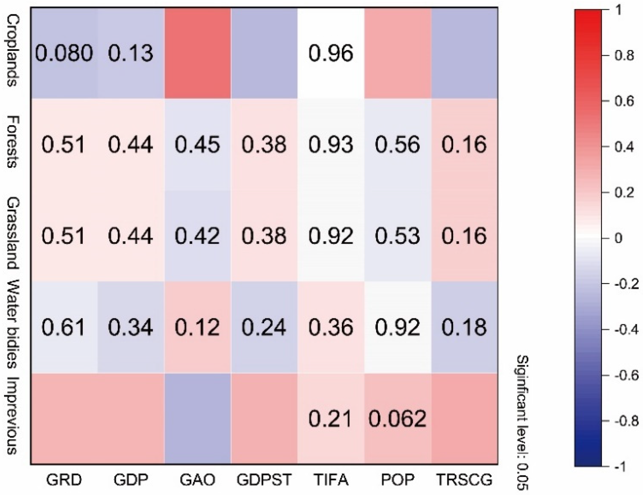
Separate correlation analysis models were constructed in this work using each socio-economic factor in turn with different LUCC types and selected the type that was most relevant to each factor. Figure 3 revealed that the impervious surface type correlated the most with GRD (p < 0.05, $\mathrm{r}$ = 0.268), GDP (p < 0.05, $\mathrm{r}$ = 0.263), GDPST (p < 0.01, $\mathrm{r}$ = 0.298), and TIFA ($\mathrm{r}$ = 0.158), whereas the cropland type was selected to match the POP (p < 0.01, $\mathrm{r}$ = 0.307), GAO (p < 0.01, $\mathrm{r}$ = 0.529), and TRSCG (p < 0.05, $\mathrm{r}$ = −0.252). In addition, the SLR results of CERA factor selected the final model with only the forests type as the independent variables, which meant forests can explain the CERA factor well (p < 0.01, $R^2$ = 0.632).

With the aim of facilitating regression models with NDVI, we gridded socio-economic factors at a resolution of 1 km by the area weighting method combined with the results of the above correlation analysis (Figure S1). Eight socio-economic factors generally showed a noticeable increasing trend from 2000 to 2015. All the factors changed somewhat differently in each district, although they generally concentrated in the center areas, except for CERA, TRSCG, and POP, which were more distributed in the surrounding areas and changed marginally over 2000 to 2015. We observed that the urbanization expanded in varying degrees and direction toward the center of study areas, such as Jianghan, Jiangan, and Huangpi districts. Furthermore, Figure S1 showed rapid increases in per capital economic benefits in urban center for 20 years from 2000 to 2020, and the results were basically the same as the trend induced by urbanization and economic development policies.

In addition, we further analyzed the land-use changes in the study area from 2000 to 2020.

Table 1. LUCC types transfer matrix of the years 2000 and 2020.

Area (2000, km2)	Area (2020, km2)
	Croplands	Forest	Grasslands	Water	Impervious	Others	Total
Croplands		22.96	1.71	99.33	425.49	2.39	551.88
Forest	18.84		1.38	4.29	18.67	0.21	43.39
Grasslands	1.58	1.68		4.66	4.48	0.26	12.66
Water bodies	46.66	3.37	2.45		66.11	3.51	122.10
Impervious	25.70	1.90	0.26	9.29		0.31	37.46
Others	2.28	0.18	0.07	4.83	4.00		11.36
Total	95.06	30.10	5.87	122.40	518.74	6.67	778.85

showed that cropland was a heavily encroached land use type, of which 77% has been converted to impervious surfaces and 18% to water bodies. The impervious surface was the most expansive type of land use, of which 50% was occupied by croplands, 40% by water bodies, 20% by forest, and 10% by grassland.

3.2. Major Factors’ Contribution Assessment

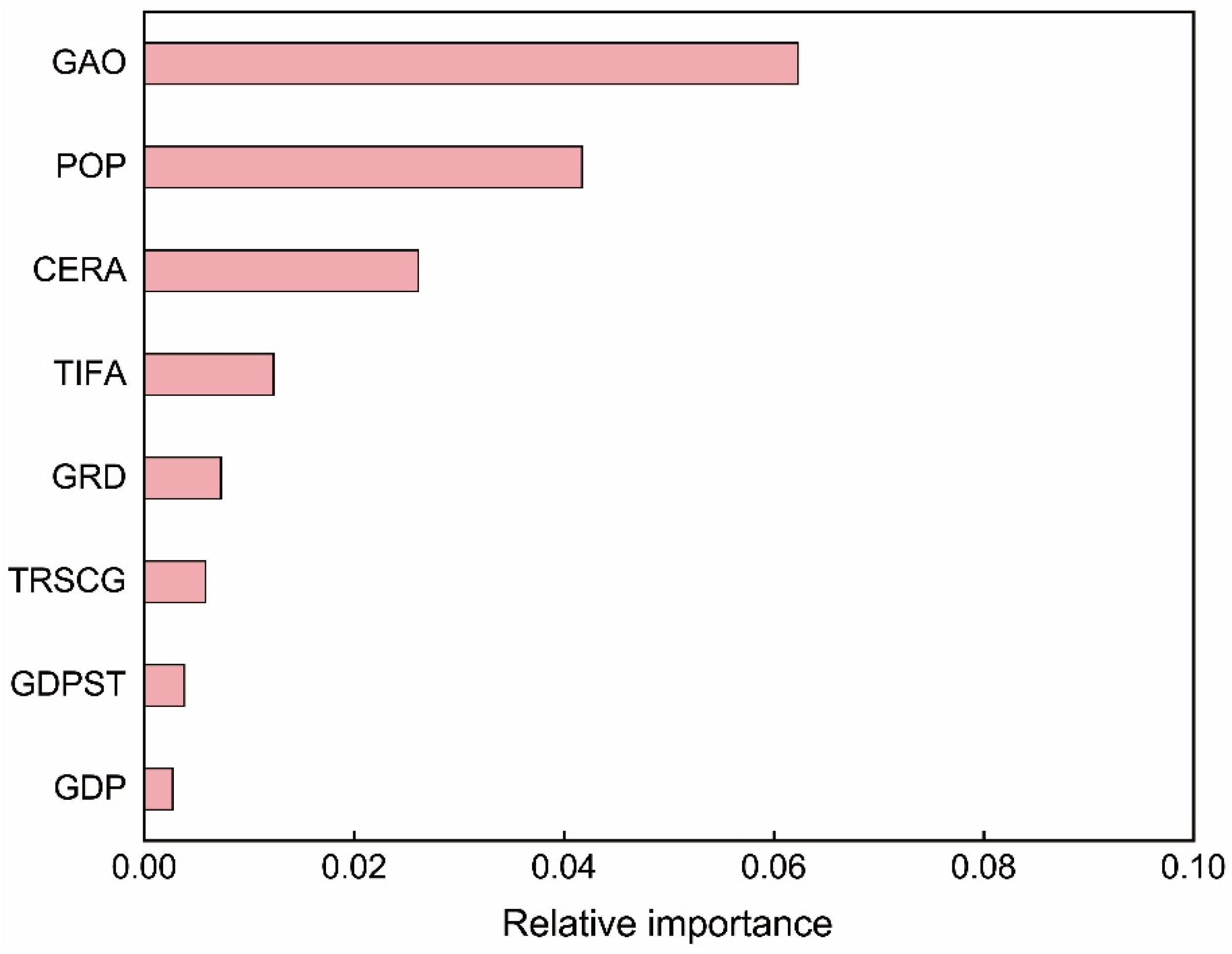
The RFR model was constructed to screen the socio-economic factors that contributed significantly to NDVI. In this selection process, the NDVI data from 2000 to 2020 were set as the dependent variables, and the socio-economic factors were the eigenvalues of the model ($R^2$ of validation set = 0.61, MSE = 0.01, parameter default). The model results demonstrated that GAO and POP factors had the greatest contribution to NDVI (Figure 4).

After feature selection using RFR, we conducted some exploratory experiments to analyze whether to continue building simplified RFR, GWR, or SGWR models for the subsequent analysis between major factors and NDVI.

Table 2. Comparison of key judging indicators between RFR and GWR.

Year	Model	MSE	R2
2000	GWR	0.006	0.64
	RFR	0.010	0.39
2005	GWR	0.008	0.65
	RFR	0.013	0.42
2010	GWR	0.009	0.67
	RFR	0.013	0.52
2015	GWR	0.013	0.61
	RFR	0.022	0.35
2020	GWR	0.016	0.59
	RFR	0.028	0.29

showed that the R² of the test set of the RFR model did not exceed 0.5, while the R² of GWR was higher than 0.5 for all. The MSEs of both were not significantly different. We finally chose GWR according to Table 2 and

Table 3. Geographical variability test results for factors.

Year	Factor	DIFF of Criterion	Geographical Variability
2000	POP	−3695.16	√
	GAO	−10,758.93	√
2005	POP	−214.69	√
	GAO	−318.15	√
2010	POP	−709.31	√
	GAO	−2272.61	√
2015	POP	−361.90	√
	GAO	−440.05	√
2020	POP	−366.56	√
	GAO	−283.35	√

. Table 3 showed that the standard deviations (denoted as DIFF) of the factors were all negative and didn’t vary over time. Thus, we selected GWR accordingly for further detailed analysis of the relationship between vegetation dynamics and major human activities.

Since the diagnostic power of the GWR model is lower, it must first be supplemented with an OLS model. The results (Table S1) of OLS showed only mild collinearity in all models every five years from 2000 to 2020 (VIF < 5, p < 0.01). We also observed that the most influential factor on NDVI was GAO factor, by comparing the absolute magnitude of standardized coefficients of the independent variables in regression results. Especially in 2005, the NDVI increased by 0.549 units for each additional GAO value, thereby keeping other conditions constant.

Furthermore, Moran’ I has been used to pre-test the spatial correlation of NDVI before applying the GWR model analysis [27,40]. Results showed the Moran’ I value during the study period were 0.80, 0.81, 0.80, 0.81, and 0.78, revealing a strong clustering pattern of NDVI in study regions.

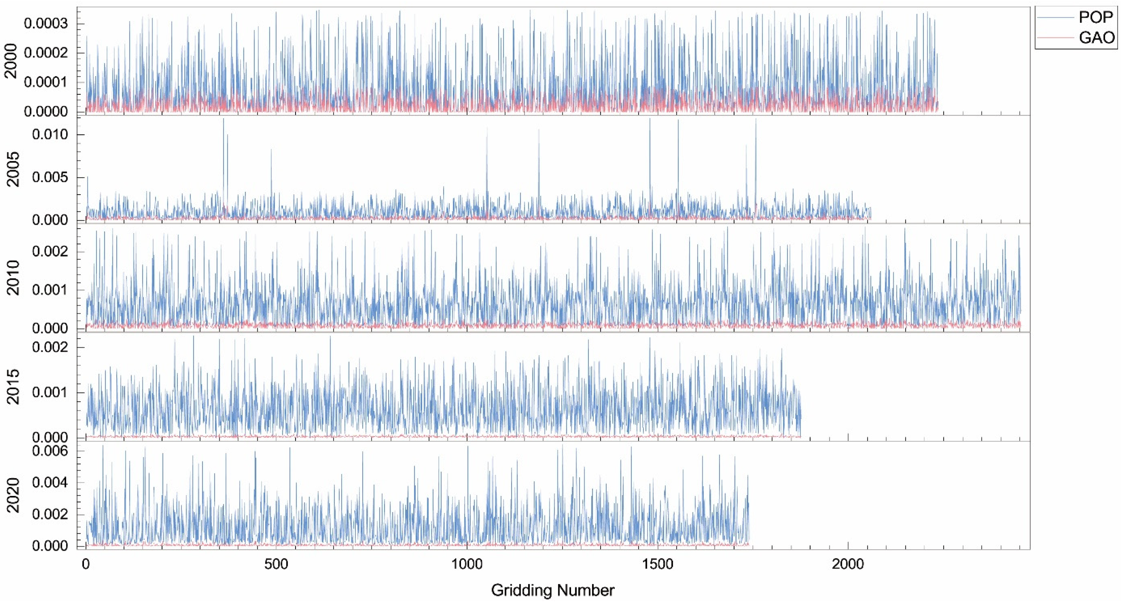
The GWR with Gauss function was configured with an annual average NDVI as the dependent variable and two vital factors in the corresponding years as the independent variables. Among the results of the GWR model (

Table 4. The overall minimum, maximum, mean, percentage of positive values, and percentage of negative values of the local estimated coefficients in the GWR models.

Year	Factor	Min	Max	Mean	Positive/%	Negative/%	Moran’ I	Z
2000	POP	−0.000345	0.000348	0	58.80	41.19	0.97	127.04
	GAO	−0.000089	0.000096	0.000001	59.85	40.15	0.97	127.23
2005	POP	−0.003956	0.011951	−0.000169	64.21	35.79	0.85	111.53
	GAO	−0.002043	0.001081	0.000023	64.57	35.43	0.85	111.53
2010	POP	−0.00203	0.002657	0.000218	75.70	24.30	0.87	91.72
	GAO	−0.00024	0.000294	−0.000019	24.32	75.68	0.87	91.92
2015	POP	−0.002264	0.001864	0.000067	61.89	38.11	0.95	98.27
	GAO	−0.000102	0.000089	−0.000004	38.22	61.78	0.95	98.28
2020	POP	−0.002966	0.006459	0.000307	64.08	35.92	0.95	124.48
	GAO	−0.000351	0.000161	−0.000017	36.10	63.90	0.95	124.46

), each local estimated coefficient represented the influence of a factor on NDVI over the local regions and a positive number means a favorable effect [29]. To divide the local estimated coefficient data into valid and invalid components, we used the adjusted critical t-values to define significance, and the original significance level was 0.05. This step could solve the problem of multiple hypothesis testing in GWR [41]. Results showed the positive and negative effects of POP and GAO factors on NDVI, suggesting some temporal heterogeneity in the relative influences of human activities on NDVI. The proportion of positive local estimated coefficients for the POP factor had always been dominant and reached the highest value of 75.70% in 2010. Meanwhile, the GAO factor began with predominantly positive coefficients, but the share of negative coefficients increased significantly after 2010.

3.3. Spatial Correlation of Major Factors with NDVI

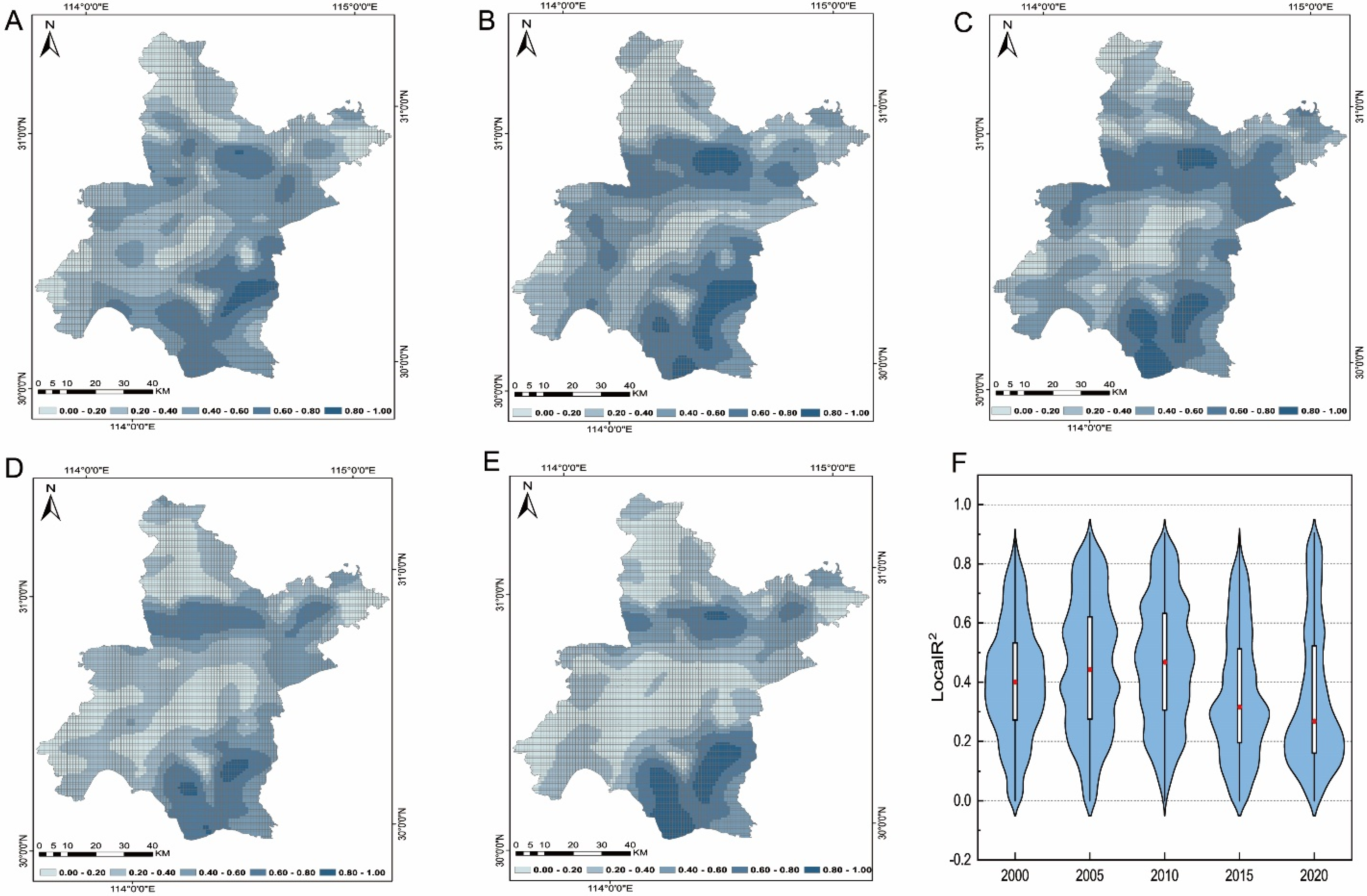
The GWR model was used to extract the spatial characteristics of human activities interacting with vegetation, which can explain the dependent variable at a local level compared with other models, and the explanation ability was represented by the local regression coefficient (LocalR²). It captured the goodness of fit of the local model (i.e., the extent to which POP and GAO jointly affect NDVI). Moreover, the spatial visualization of LocalR² could make the spatial heterogeneity of this effect more intuitive. The LocalR² in Figure 5 ranged from 0.6 to 0.8 in Jiangxia district and southern Huangpi district, thereby indicating a remarkable association between NDVI and the two major drivers (e.g., POP and GAO) in these areas. By contrast, a low LocalR² and a negligible association between NDVI and two drivers existed in the urban center regions, such as Jiangan, Wuchang, Qingshan, and Jiangxia districts. Overall, it showed a circular feature, with low correlation in the middle and around and greater correlation in the urban–rural interface area located in between.

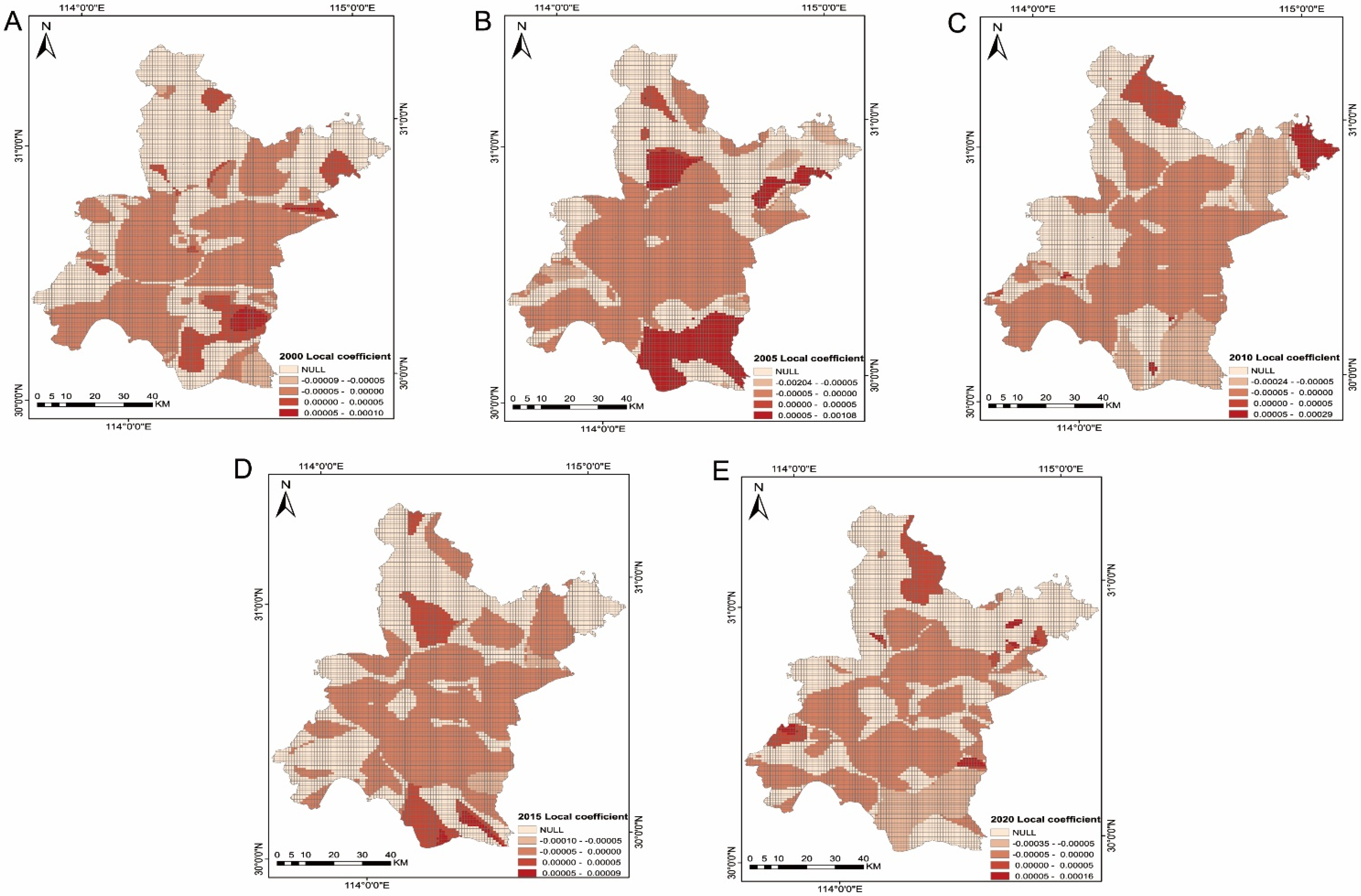
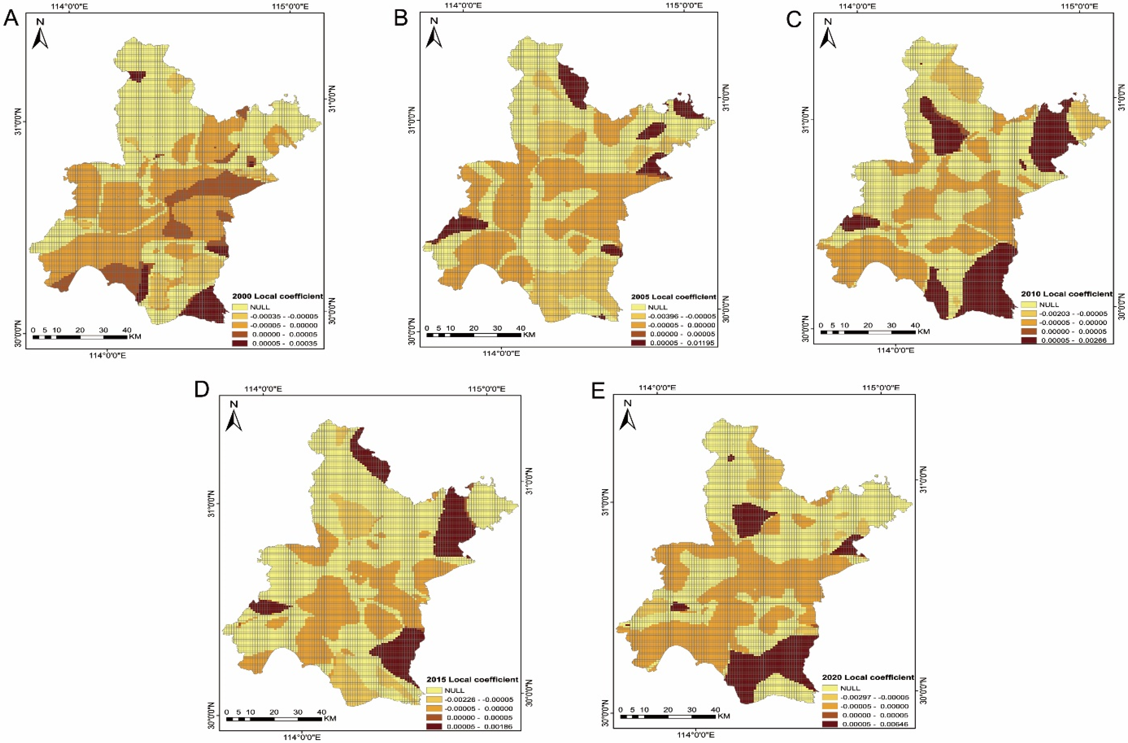
The local estimated coefficients of factors that passed the 0.05 significance test for approximately 8980 grids were visualized on the administrative map to intuitively identify varying directions and spatial characteristics. The results demonstrated obvious geospatial heterogeneity in the estimated coefficients of variations for all five years, because regardless of whether a positive or negative correlation exists between two drivers and NDVI, and the strength of both relationships varied according to spatial variations. This is similar to the outcomes of Ma Bo et al., who all found that the impact of human activities on vegetation varied with spatial variation [19,37].

As shown in Figure 6, fewer regions had positive coefficients of the GAO factor, which indicated that negative effects played an increasingly strong role in the contribution of the GAO factor to NDVI. Meanwhile, we also noticed that the areas that passed the significance test were mostly rivers, lakes, and wetlands.

Figure 7 illustrates that the spatial distribution of estimated coefficients of the POP factor was somewhat like that of the GAO. The distribution pattern of negative estimated coefficients in urban centers showed that population density was closely related to vegetation coverage reduction. Because the increasing population led to an accompanying increase in the construction of urban facilities [23], which can dramatically occupy vegetated land. By contrast, the positive values of coefficients were usually distributed in the peripheral areas, such as Jiangxia District and parts of Xinzhou District, where the population outflow accounted for the significant differences from the center regions.

Furthermore, we used the factor with the largest absolute value of coefficients for each grid as the principal driver influencing NDVI in local areas, which was beneficial for generating the spatial distribution of prevailing factors that affected vegetation. However, by comparing the absolute values of the estimated coefficients of two main drivers for each grid, we observed that the driver with larger absolute values in all grids was the POP factor (Figure 8). It indicated that for the whole study area, the main driver that affected NDVI was the POP factor, and the variability of the dominant factor’s spatial distribution was insignificant.

4. Discussion

4.1. Driving Factors of Vegetation Coverage

For urban ecosystems, climatic factors were not the most significant factors that influenced vegetation coverage at the interannual scale. Previous studies shown that climatic factors were usually the controlling force for seasonal variation in vegetation growth [1,7]. In the analysis of interannual variability, climatic factors did not have a substantial effect on regional vegetation because extreme weather did not occur frequently [3]. A growing number of studies have found that human activities were gradually becoming the determinant factors that affect vegetation coverage in areas with marked vegetation greening [19,36,37]. Therefore, separately quantifying the potential impact of human activities on vegetation at the interannual scale is of significance. Based on this conclusion, the general experimental ideas of our study were derived. We first selected eight socio-economic factors for regression analysis with NDVI. Also, area-weighted interpolation was used to objectively redistribute the spatial distribution of socio-economic factors in combination with LUCC data. Then, some corresponding quantitative models were used to jointly assess the hidden relationship between human activities and vegetation directly. The results obtained from the experiments also confirmed the validity of the above conclusions.

In the findings of this study, GAO and POP factors stood out from the contribution assessment of eight factors to NDVI. Together, these two factors were able to contribute up to more than 50% of NDVI. Moreover, the comparison between GAO and the POP factor demonstrated that POP was the most prominent factor that affects NDVI. Specifically, the influence of POP on NDVI showed a shifting tendency from a negative to positive correlation from 2000 to 2020. The GAO factor was the opposite, thereby showing a trend from a positive to a negative correlation (Table 4). The turning point of these two factors was both 2010. This interesting finding is similar to that of Yongzhe Chen et al. They found that during the 2001–2018 period, vegetation productivity in China showed a significant turnaround in 2010 under the influence of human activities and climatic factors, mainly due to the continuous improvement of uncontrollable climatic conditions [31].

In order to further consider the manifestation of human activities on land use, we inspected the land use changes in the study from 2000 to 2020. Table 1 illustrates that the areas of forests and grasslands had not significantly changed, while the areas of croplands decreased by 456.82 km², of which 77% was converted into impervious. These indicated that with the urbanization of the study area, many croplands, mainly in the central area, have been occupied for 20 years [14,35]. However, the overall human impact on NDVI gradually shows a positive effect, showing that good agricultural production and the implementation of environmental protection measures in the urban fringe and urban-rural areas can offset the negative impact on the central urban areas. This phenomenon might be explained by the fact that although agricultural production and population was often considered the main driver of environmental damage, it was also an important force in managing agricultural land to avoid vegetation destruction and in implementing environmental protection measures.

4.2. Quantitative Evaluation Models

The RFR, OLS, and GWR models were used in our study to collectively assist in assessing the potential contribution of drivers to vegetation. Given that machine learning algorithms were able to address the numerous non-linear and uncertain effects between socio-economic factors and NDVI well [15,18], the RFR was used initially to select the two dominant factors to simplify the model for subsequent detailed analysis. The OLS model was then employed with the aim of diagnosing the model’s feasibility, although its fit was far inferior to the other models. Lastly, for each year (2000, 2005, 2010, 2015, 2020), a detailed spatial analysis with major factors (e.g., POP and GAO) and NDVI was performed using the GWR model, which uses a spatial weighting function to map the overall problem to a local space to obtain local regression results.

In fact, after using RFR for feature selection, we performed some additional experiments to explore whether to continue building the simplified machine learning models (RFR) or to use the linear regression models (GWR or SGWR) for the subsequent analysis between the two factors (e.g., POP and GAO) and NDVI. The results (Table 2) showed that the fitting performance of the RFR was not necessarily better than that of the GWR model for data sets with low data volume and few features. However, the results of both methods all indicated that the POP factor contributes more to NDVI compared with the GAO factor. Therefore, the GWR model was more suitable for the subsequent analysis in this study.

Within traditional regression methods, the SGWR model was also often used for the assessment of vegetation drivers. It was used to solve the simultaneous problems of spatial heterogeneity and homogeneity in this study. Whether they required SGWR model was based on the geographic variability test (GVT), the DIFF values from Table 3 were used to directly determine the geographic variability of factors [29]. Positive DIFF values indicated that the corresponding variable did not have geographic variability. Otherwise, it meant that the variable had geographic spatial heterogeneity. The use of SGWR instead of the GWR model was necessary only when the model included both factors with positive DIFF values and factors with negative DIFF values to improve the model performance. The principal formula of the SGWR model was calculated as:

$$y_i={\beta }_0\left(u_i,v_i\right)+{\displaystyle \sum }_{l=1}^j{\alpha }_l{x}_{il}+{\displaystyle \sum }_{k=j+1}^p{\beta }_k\left(u_i,v_i\right)x_{ik}+{\epsilon }_i$$

(9)

where $\left(u_i,v_i\right)$ represents the geographic coordinates of the ith point, $x_{il}$ and ${\alpha }_l$ represent the value of independent variable and its estimation of global regression, respectively; ${\beta }_k\left(u_i,v_i\right)$ represents the local regression estimate of the kth independent variable at location $i$. ${\beta }_0\left(u_i,v_i\right)$ and ${\epsilon }_i$ represent the intercept and error estimate term for location $i$, respectively; and ${\beta }_k\left(u_i,v_i\right)$ was a function of geography estimating by the weighted least square method.

Table 3 indicated that POP and GAO factors all had negative DIFF values, which meant that they all had the geographic spatial heterogeneity in our studies. Thus, it was a meaningless procedure to further improve the accuracy using the SGWR model.

4.3. Spatial Characteristic of the Impact of Human Activities on NDVI

The GWR model was a useful way to understand spatial properties. For one thing, the coupling process among socio-economic factors (e.g., POP and GAO) and NDVI has spatial heterogeneity (Figure 5). Based on the context of different regions, the effectiveness of socio-economic factors on vegetation coverage varied in spatial terms, which was consistent with the conclusion of Jiang Meichen et al. [5,19,37]. The local estimated coefficients of POP and GAO factors exhibited the same spatial distribution characteristics. In other words, the coefficients gradually switched from negative to positive values along with the geographic location from the center of the area to the periphery. In addition, the spatial patterns of the coupling of human activities and the eco-environment all formed an approximate circular structure. Human activities and vegetation also have a strong correlation in the interface areas between urban centers and fringe areas, which is similar to the findings of Jin Kai et al. [10,16].

Furthermore, the spatial differentiation of major local drivers was not apparent because the NDVI was most influenced by the POP factor in all gridding areas in this study (Figure 8). However, ref. [3] discovered that the main drivers of vegetation coverage vary in each region of China with significant regional variability. Such a contradiction could be explained by two reasons. One was that we considered only anthropogenic factors and ignored other factors, such as climate or topography. The other was closely related to the size of the study regions. That is, the effects and research findings on a large scale did not necessarily occur in a small-scale region.

4.4. Limitations

In this study, the approach to quantifying human activities was to select several socio-economic factors. However, statistics on these factors based on administrative units were unstable because the division of zoning units on which the yearbook data based changed annually, and the residents of study areas did not report data directly to government agencies. Moreover, other factors that were unavailable in the yearbooks but also closely related to vegetation coverage, such as real-time population migration data and carbon emission data, were not considered. The most critical measure for follow-up research is to construct a standard evaluation system of human activity based on specific research areas using more accurate data on anthropogenic factors and based on the conditions of study areas.

The spatialization model of socio-economic factors was constructed by using only LUCC data, and the values of factors were interpolated using weighted areas. As a result, the spatialization of factors was not very accurate. Subsequent studies will consider more multi-source data related to human activities, such as nighttime lighting, social perception, and urban vehicle movement trajectory data. A more complex and accurate mathematical spatialization model will also be constructed.

Considering that LUCC data were only available every five years, the coupling analysis models for our study were limited to four years, specifically 2000, 2005, 2010, 2015, and 2020. Such instances resulted in the inability to conduct continuous spatiotemporal analysis. Therefore, subsequent studies will not be limited to four years. We would like to further validate the current findings using year-by-year remote sensing data and more comprehensive quantitative data related to human activities by considering longer time periods and more urban areas.

5. Conclusions

We utilized remote sensing images, and socio-economic and land use classification data to quantify the intensity of human activity and vegetation coverage in Wuhan from 2000 to 2020. We also set up the experimental ideas based on the respective strengths of traditional linear regressions and machine learning methods, and some interesting results were obtained in this study, which could facilitate a more accurate explanation of the potential relationships between human activities and vegetation. First, GWR is more appropriate than RFR for regression analysis of a small set of key factors with NDVI because the difference in precision between them is minor and RFR lacks a more mechanistic interpretation of the issue. Second, there was a strong synergistic positive relevance between human activity and urban vegetation. According to the mathematical results of models, potential socio-economic factors as a whole could explain more than half of the vegetation cover. And a very significant conclusion was obtained that vegetation in urban-rural interface areas was more vulnerable to human activities. Lastly, the POP and GAO were the dominant factors influencing NDVI. This study confirmed that the correlation between socioeconomic factors and NDVI was significantly spatially heterogeneous and varied over time. All in all, human activities have been observed to play a non-negligible role in the increase in vegetation coverage in the balance of urbanization and environmental protection policies.

We would suggest enhancing reforestation and greening management in suburban areas for better urban environmental protection. Optimizing suburban infrastructure sequentially leads the population to the suburbs, where they can engage in productive work in agriculture and forestry. This will not only reduce the population pressure in urban centers but also, to a certain extent contribute to the environmental conditions of the whole city. The outcomes of our study can also be beneficial for helping policy makers to understand the impact of human activities on the ecological environment more clearly and to adjust their strategies in time.

References

1. Xin, Z.; Xu, J.; Zheng, W. Spatiotemporal variations of vegetation cover on the Chinese Loess Plateau (1981–2006): Impacts of climate changes and human activities. Sci. China Ser. D Earth Sci. 2008, 51, 67–78. [Google Scholar] [CrossRef]
2. Lu, D.; Xu, X.; Tian, H.; Moran, E.; Zhao, M.; Running, S. The Effects of Urbanization on Net Primary Productivity in Southeastern China. Environ. Manag. 2010, 46, 404–410. [Google Scholar] [CrossRef] [PubMed]
3. Feng, Q.; Ma, H.; Jiang, X.; Wang, X.; Cao, S. What Has Caused Desertification in China? Sci. Rep. 2015, 5, 15998. [Google Scholar] [CrossRef] [PubMed] [Green Version]
4. Shen, Q.; Gao, G.; Han, F.; Xiao, F.; Ma, Y.; Wang, S.; Fu, B. Quantifying the effects of human activities and climate variability on vegetation cover change in a hyper-arid endorheic basin. Land Degrad. Dev. 2018, 29, 3294–3304. [Google Scholar] [CrossRef]
5. Jiang, M.; Tian, S.; Zheng, Z.; Zhan, Q.; He, Y. Human Activity Influences on Vegetation Cover Changes in Beijing, China, from 2000 to 2015. Remote Sens. 2017, 9, 271. [Google Scholar] [CrossRef] [Green Version]
6. Jin, J.; Gergel, S.E.; Lu, Y.; Coops, N.C.; Wang, C. Asian Cities are Greening While Some North American Cities are Browning: Long-Term Greenspace Patterns in 16 Cities of the Pan-Pacific Region. Ecosystems 2020, 23, 383–399. [Google Scholar] [CrossRef]
7. Yao, R.; Cao, J.; Wang, L.; Zhang, W.; Wu, X. Urbanization effects on vegetation cover in major African cities during 2001–2017. Int. J. Appl. Earth Obs. Geoinf. 2019, 75, 44–53. [Google Scholar] [CrossRef]
8. Foley, J.A.; DeFries, R.; Asner, G.P.; Barford, C.; Bonan, G.; Carpenter, S.R.; Chapin, F.S.; Coe, M.T.; Daily, G.C.; Gibbs, H.K.; et al. Global consequences of land use. Science 2005, 309, 570–574. [Google Scholar] [CrossRef] [Green Version]
9. Kaufmann, R.K.; Seto, K.C.; Schneider, A.; Liu, Z.; Zhou, L.; Wang, W. Climate response to rapid urban growth: Evidence of a human-induced precipitation deficit. J. Clim. 2007, 20, 2299–2306. [Google Scholar] [CrossRef]
10. Zhang, C.; Tian, H.; Pan, S.; Liu, M.; Lockaby, G.; Schilling, E.B.; Stanturf, J. Effects of Forest Regrowth and Urbanization on Ecosystem Carbon Storage in a Rural-Urban Gradient in the Southeastern United States. Ecosystems 2008, 11, 1211–1222. [Google Scholar] [CrossRef]
11. Chen, C.; Park, T.; Wang, X.; Piao, S.; Xu, B.; Chaturvedi, R.K.; Fuchs, R.; Brovkin, V.; Ciais, P.; Fensholt, R.; et al. China and India lead in greening of the world through land-use management. Nat. Sustain. 2019, 2, 122–129. [Google Scholar] [CrossRef] [PubMed]
12. Liu, Y.; Xu, Z. A Study of Spatialization Methods of Human Factors Based on IPAT Model. J. Glaciol. Geocryol. 2012, 34, 740–747. [Google Scholar]
13. Liu, H.; Zheng, L.; Liao, M. Dynamics of Vegetation Change and Its Relationship with Nature and Human Activities—A Case Study of Poyang Lake Basin, China. J. Sustain. For. 2021, 40, 47–67. [Google Scholar] [CrossRef]
14. Mueller, T.; Dressler, G.; Tucker, C.J.; Pinzon, J.E.; Leimgruber, P.; Dubayah, R.O.; Hurtt, G.C.; Bohning-Gaese, K.; Fagan, W.F. Human Land-Use Practices Lead to Global Long-Term Increases in Photosynthetic Capacity. Remote Sens. 2014, 6, 5717–5731. [Google Scholar] [CrossRef] [Green Version]
15. Shi, Y.; Jin, N.; Ma, X.; Wu, B.; He, Q.; Yue, C.; Yu, Q. Attribution of climate and human activities to vegetation change in China using machine learning techniques. Agric. For. Meteorol. 2020, 294, 108146. [Google Scholar] [CrossRef]
16. Jin, K.; Wang, F.; Li, P. Responses of Vegetation Cover to Environmental Change in Large Cities of China. Sustainability 2018, 10, 270. [Google Scholar] [CrossRef] [Green Version]
17. Wu, Z.; Li, Z.; Zeng, H. Using Remote Sensing Data to Study the Coupling Relationship between Urbanization and Eco-Environment Change: A Case Study in the Guangdong-Hong Kong-Macao Greater Bay Area. Sustainability 2020, 12, 7875. [Google Scholar] [CrossRef]
18. Leroux, L.; Begue, A.; Seen, D.L.; Jolivot, A.; Kayitakire, F. Driving forces of recent vegetation changes in the Sahel: Lessons learned from regional and local level analyses. Remote Sens. Environ. 2017, 191, 38–54. [Google Scholar] [CrossRef] [Green Version]
19. Wu, S.P.; Gao, X.; Lei, J.Q.; Zhou, N.; Wang, Y.D. Spatial and Temporal Changes in the Normalized Difference Vegetation Index and Their Driving Factors in the Desert/Grassland Biome Transition Zone of the Sahel Region of Africa. Remote Sens. 2020, 12, 4119. [Google Scholar] [CrossRef]
20. Hunter, L.M. People and pixels: Linking remote sensing and social science. Contemp. Sociol. J. Rev. 1999, 28, 362–363. [Google Scholar] [CrossRef]
21. Gaffin, S.R.; Rosenzweig, C.; Xing, X.S.; Yetman, G. Downscaling and geo-spatial gridding of socio-economic projections from the IPCC Special Report on Emissions Scenarios (SRES). Glob. Environ. Chang. 2004, 14, 105–123. [Google Scholar] [CrossRef]
22. Brinegrar, S.J.; Popick, S.J. A Comparative Analysis of Small Area Population Estimation Methods. Cartogr. Geogr. Inf. Sci. 2010, 37, 273–284. [Google Scholar] [CrossRef]
23. Zhuo, L.; Ichinose, T.; Zheng, J.; Chen, J.; Shi, P.J.; Li, X. Modelling the population density of China at the pixel level based on DMSP/OLS non-radiance-calibrated night-time light images. Int. J. Remote Sens. 2009, 30, 1003–1018. [Google Scholar] [CrossRef]
24. Han, X.; Zhou, Y.; Wang, S.; Liu, R.; Yao, Y. GDP Spatialization in China based on DMSP/OLS Data and Land Use Data. Remote Sens. Technol. Appl. 2012, 27, 396–405. [Google Scholar]
25. Lu, D.; Weng, Q.; Li, G. Residential population estimation using a remote sensing derived impervious surface approach. Int. J. Remote Sens. 2006, 27, 3553–3570. [Google Scholar] [CrossRef]
26. Peng, C.; Jin, X.; Wong, K.-C.; Shi, M.; Lio, P. Collective Human Mobility Pattern from Taxi Trips in Urban Area. PLoS ONE 2012, 7, e34487. [Google Scholar] [CrossRef] [Green Version]
27. Li, J.; Yan, Q.; Hu, M. Spatial-Temporal Evolution of Vegetation and Dominant Factors inEnergy Golden TriangleRegion Based on Geographically Weighted Regression Model. J. Ecol. Rural Environ. 2018, 34, 700–708. [Google Scholar]
28. Shi, S.; Yu, J.; Wang, F.; Wang, P.; Zhang, Y.; Jin, K. Quantitative contributions of climate change and human activities to vegetation changes over multiple time scales on the Loess Plateau. Sci. Total Environ. 2021, 755, 142419. [Google Scholar] [CrossRef]
29. Jin, Y.; Zhang, H.; Yan, Y.; Cong, P. A Semi-Parametric Geographically Weighted Regression Approach to Exploring Driving Factors of Fractional Vegetation Cover: A Case Study of Guangdong. Sustainability 2020, 12, 7512. [Google Scholar] [CrossRef]
30. Peng, J.; Li, Y.; Tian, L.; Liu, Y.; Wang, Y. Vegetation Dynamics and Associated Driving Forces in Eastern China during 1999–2008. Remote Sens. 2015, 7, 13641–13663. [Google Scholar] [CrossRef] [Green Version]
31. Chen, Y.Z.; Feng, X.M.; Tian, H.Q.; Wu, X.T.; Gao, Z.; Feng, Y.; Piao, S.L.; Lv, N.; Pan, N.Q.; Fu, B.J. Accelerated increase in vegetation carbon sequestration in China after 2010: A turning point resulting from climate and human interaction. Glob. Chang. Biol. 2021, 27, 5848–5864. [Google Scholar] [CrossRef] [PubMed]
32. Zaimes, G.N.; Gounaridis, D.; Symenonakis, E. Assessing the impact of dams on riparian and deltaic vegetation using remotely-sensed vegetation indices and Random Forests modelling. Ecol. Indic. 2019, 103, 630–641. [Google Scholar] [CrossRef]
33. Clauss, K.; Ottinger, M.; Leinenkugel, P.; Kuenzer, C. Estimating rice production in the Mekong Delta, Vietnam, utilizing time series of Sentinel-1 SAR data. Int. J. Appl. Earth Obs. Geoinf. 2018, 73, 574–585. [Google Scholar] [CrossRef]
34. Huang, S.; Zheng, X.; Ma, L.; Wang, H.; Huang, Q.; Leng, G.; Meng, E.; Guo, Y. Quantitative contribution of climate change and human activities to vegetation cover variations based on GA-SVM model. J. Hydrol. 2020, 584, 124687. [Google Scholar] [CrossRef]
35. Luo, D.; Goodin, D.G.; Caldas, M.M. Spatial-Temporal Analysis of Land Cover Change at the Bento Rodrigues Dam Disaster Area Using Machine Learning Techniques. Remote Sens. 2019, 11, 2548. [Google Scholar] [CrossRef] [Green Version]
36. Hua, W.J.; Chen, H.S.; Zhou, L.M.; Xie, Z.H.; Qin, M.H.; Li, X.; Ma, H.D.; Huang, Q.H.; Sun, S.L. Observational Quantification of Climatic and Human Influences on Vegetation Greening in China. Remote Sens. 2017, 9, 425. [Google Scholar] [CrossRef] [Green Version]
37. Ma, B.; Wang, S.S.; Mupenzi, C.; Li, H.R.; Ma, J.Y.; Li, Z.B. Quantitative Contributions of Climate Change and Human Activities to Vegetation Changes in the Upper White Nile River. Remote Sens. 2021, 13, 3648. [Google Scholar] [CrossRef]
38. Dong, J. Study on the progress of spatialization of anthrop factors. J. Gansu Sci. 2007, 19, 91–94. [Google Scholar]
39. Breiman, L. Random forests. Mach. Learn. 2001, 45, 5–32. [Google Scholar] [CrossRef] [Green Version]
40. Yu, H.R.; Gong, H.L.; Chen, B.B.; Liu, K.S.; Gao, M.L. Analysis of the influence of groundwater on land subsidence in Beijing based on the geographical weighted regression (GWR) model. Sci. Total Environ. 2020, 738, 139405. [Google Scholar] [CrossRef]
41. da Silva, A.R.; Fotheringham, A.S. The Multiple Testing Issue in Geographically Weighted Regression. Geogr. Anal. 2016, 48, 233–247. [Google Scholar] [CrossRef]
Figure 1. (A) Hubei Province in China, (B) Wuhan City in Hubei Province, and (C) Wuhan City divided into thirteen districts.
Remotesensing 14 02999 g001
Figure 2. Research framework.
Remotesensing 14 02999 g002
Figure 3. Correlation analysis of seven social factors with LUCC types.
Remotesensing 14 02999 g003
Figure 4. Assessment of the contributions of all socio-economic factors to NDVI from 2000 to 2020.
Remotesensing 14 02999 g004
Figure 5. Spatial distributions of LocalR2 in Wuhan in 2000 (A), 2005 (B), 2010 (C), 2015 (D) and 2020 (E) at a gridding resolution of 1 km based on GWR model (F).
Remotesensing 14 02999 g005
Figure 6. (AE) Local estimated coefficients for GAO of NDVI in Wuhan at a gridding resolution of 1 km calculated by GWR.
Remotesensing 14 02999 g006
Figure 7. (AE) Local estimated coefficients for POP of NDVI in Wuhan at a gridding resolution of 1 km calculated by GWR.
Remotesensing 14 02999 g007
Figure 8. Comparisons of the absolute values of local estimated coefficients of POP and GAO that passed the 0.05 significance test.
Remotesensing 14 02999 g008