Article

Self-Supervised Assisted Semi-Supervised Residual Network for Hyperspectral Image Classification

1
School of Artifical Intelligentce, Xidian University, Xi’an 710071, China
2
Guangzhou Institute of Technology, Xidian University, Xi’an 710071, China
3
Intelligent Decision and Cognitive Innovation Center, State Administration of Science, Technology and Industry for National Defense, Beijing 100048, China
*
Author to whom correspondence should be addressed.
Remote Sens. 2022, 14(13), 2997; https://doi.org/10.3390/rs14132997
Submission received: 12 May 2022 / Revised: 20 June 2022 / Accepted: 21 June 2022 / Published: 23 June 2022
(This article belongs to the Section AI Remote Sensing)

Abstract

:
Due to the scarcity and high cost of labeled hyperspectral image (HSI) samples, many deep learning methods driven by massive data cannot achieve the intended expectations. Semi-supervised and self-supervised algorithms have advantages in coping with this phenomenon. This paper primarily concentrates on applying self-supervised strategies to make strides in semi-supervised HSI classification. Notably, we design an effective and a unified self-supervised assisted semi-supervised residual network (SSRNet) framework for HSI classification. The SSRNet contains two branches, i.e., a semi-supervised and a self-supervised branch. The semi-supervised branch improves performance by introducing HSI data perturbation via a spectral feature shift. The self-supervised branch characterizes two auxiliary tasks, including masked bands reconstruction and spectral order forecast, to memorize the discriminative features of HSI. SSRNet can better explore unlabeled HSI samples and improve classification performance. Extensive experiments on four benchmarks datasets, including Indian Pines, Pavia University, Salinas, and Houston2013, yield an average overall classification accuracy of 81.65%, 89.38%, 93.47% and 83.93%, which sufficiently demonstrate that SSRNet can exceed expectations compared to state-of-the-art methods.

Graphical Abstract

1. Introduction

With the development of remote sensing and information processing technology, HSI technology has become the focus in the remote sensing community. The hyperspectral image is a precise remote sensing means that contains rich spatial texture information and spectral reflectance information [1], which has unique advantages in subtle recognition and detection missions. e.g., vegetation cover monitoring [2], atmospheric environmental research [3], and marine monitoring [4].
Based on the recent literature reviewed in [5], HSI classification is the most vibrant field of research in the hyperspectral community (i.e., each pixel in hyperspectral images is appointed a unique category). Within the initial stage of HSI classification, most methods take spectral features, such as independent component analysis (ICA) [6] and support vector machines (SVM) [7], as the primary classification basis. However, the HSI classification results obtained by these methods are unsatisfactory since the spatial features are not well exploited. Due to the characteristics of spatial homogeneity and heterogeneity and mixed pixels of HSI, it is difficult to fully utilize the features of HSI by spectral feature extraction alone. The spatial features can improve the classification performance of HSI [8]; increasingly, classification strategies that combine spatial features have been proposed. For example, a hyperspectral data preprocessing method based on mathematical morphology was proposed in [9] in which extended morphological profiles (EMPs) were utilized to exact spatial construction information through morphological manipulation.
With the rapid development of deep learning (DL) [10], DL has been presented in numerous computer vision tasks and has made worthwhile breakthroughs. As a typical deep learning(DL) model, a convolutional neural network (CNN) has been considered to create full utilization of the spatial and spectral features of HSI [11], and researchers have proposed a series of HSI classification methods based on CNN. Hu et al. [12] used a deep CNN model for HSI classification and achieved good performance. Chen et al. [13] proposed a 3D-CNN model for HSI classification, which performs superior to a 1D-CNN and a 2D-CNN. Cheng et al. [14] designed a spatial–spectral random patch network, which made adequate utilization of the spatial and spectral information and achieved satisfactory performance. However, due to the scarcity of labeled samples in HSI, DL-based strategies cannot obtain satisfactory accuracy. The collection and labeling of HSI are complicated, time-consuming, and high-cost. Therefore, the number of labeled training samples is greatly limited, and the shortage of training samples is one of the main obstacles to productive HSI classification methods.
Some recent works have begun to explore self-supervised or semi-supervised strategies for HSI classification to solve this problem. Semi-supervised learning methods aim to improve performance by simultaneously using a few labeled samples and a large number of unlabeled samples. Several semi-supervised methods have been used for HSI classification, which are roughly categorized into three classes: (1) self-training [15,16,17]; e.g., Li et al. [16] iteratively enlarged the training sample set and retrained the classifier, and the selection of training samples was based on the region information, so the risk of assigning wrong labels was primarily reduced. (2) generative models [18,19,20]; e.g., Feng et al. [19] proposed a semi-supervised dual-branch convolutional autoencoder with self-attention. (3) graph-based methods [21,22,23]; e.g., Ding et al. [23] proposed a semi-supervised locality-preserving dense graph neural network (GNN) for HSI classification in which autoregressive moving average filters and context-aware learning are integrated. Moreover, the self-supervised learning methods are also applied to the few-shot HSI classification [24,25,26,27]. In [26], a self-supervised contrastive fruitful disymmetrical expanded network is presented for HSI classification. In [27], a self-supervised learning strategy with flexible distillation is proposed for HSI classification. Nevertheless, these approaches suffer from some limitations. Self-training requires high-confidence samples with their “pseudo-labels” to update the training set, and the performance will get worse once the “pseudo-labels” are incorrect. Methods based on a graph should construct a structural graph, but it is troublesome due to the fact that the latent spatial–spectral structural information is not easy to learn.
In view of these limitations, we attempt to incorporate a self-supervised strategy into a semi-supervised framework and propose a unified SSRNet. The proposed SSRNet is designed as two branches: a semi-supervised and a self-supervised branch. The semi-supervised component consists of a residual feature extraction network (RNet) that extracts discriminative spectral–spatial features from HSI cubes. Since random perturbation is proved to be an effective way for robust classification [28,29,30,31], we implement perturbation by spectral feature shift in this framework. The self-supervised component consists of two auxiliary tasks: a spectral order forecast and a masked bands reconstruction, which can learn the discriminative features of HSI.
To summarize, the contributions of the proposed methods are threefold as follows:
(1) Self-supervised learning is integrated into a semi-supervised framework for HSI classification by designing a unified multi-task SSRNet. SSRNet has competitive performance, especially under few labeled samples conditions.
(2) A semi-supervised data random perturbation strategy is proposed. This perturbation strategy is the bidirectional movement of some randomly selected spectral segments along the spatial dimension, respectively, on the HSI feature maps.
(3) Two types of self-supervised auxiliary tasks are presented for SSRNet. The two auxiliary tasks, i.e., masked bands reconstruction and spectral order forecast, can help the network learn the discriminative features.

2. Methodology

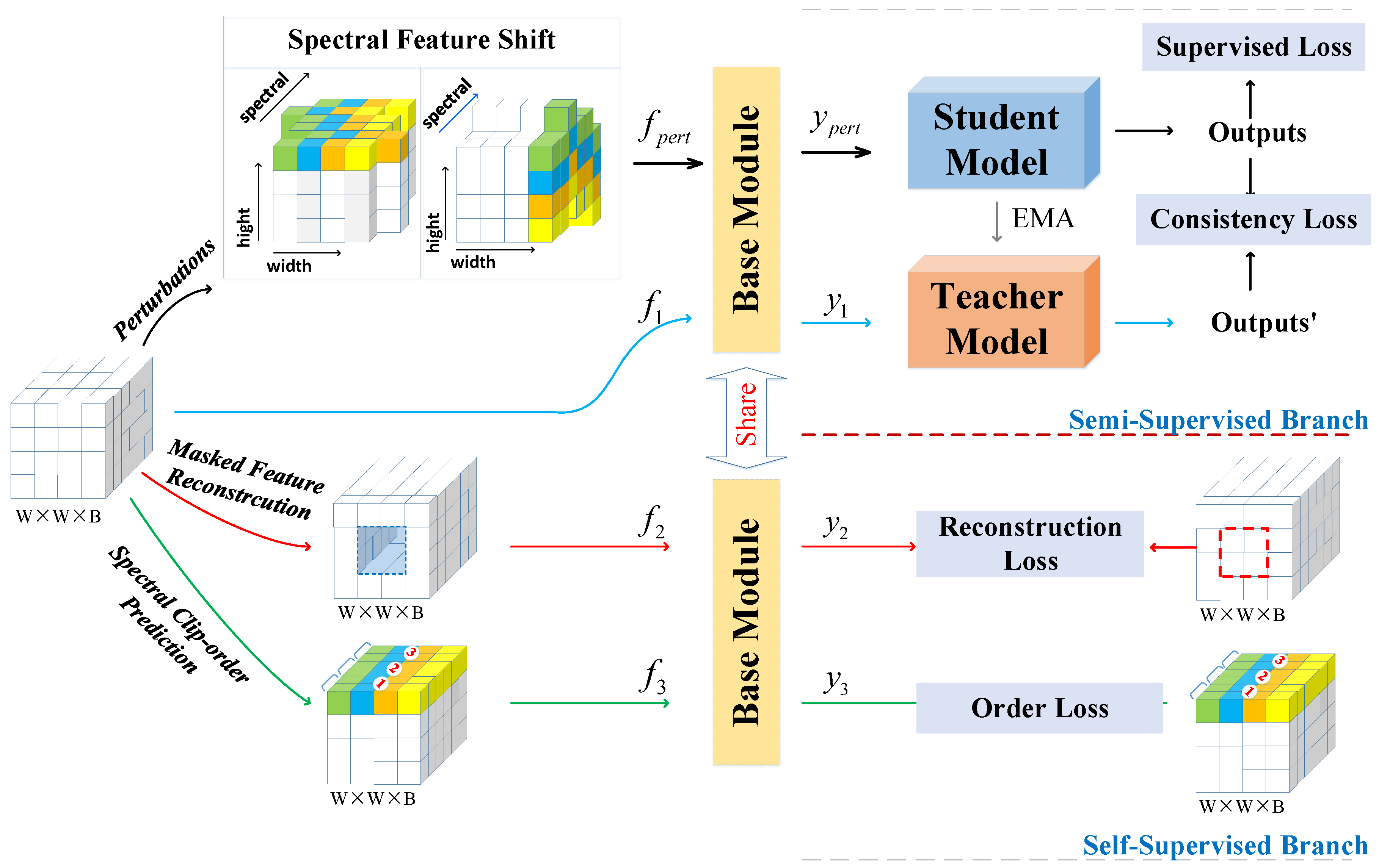
This section will present the proposed SSRNet, including the semi-supervised and self-supervised branches. In the semi-supervised branch, we amplify the mean-teacher [29] framework with one kind of random perturbation, i.e., spectral feature shift. Furthermore, we design a residual feature extraction network (RNet) for learning spectral–spatial features. In the self-supervised branch, two auxiliary tasks: masked bands reconstruction and spectral order forecast, are explored to help in training the proposed SSRNet. Figure 1 illustrates the outline of the SSRNet.

2.1. The Overall Framework of the Proposed SSRNet

The HSI data cube is denoted by D R M × N × L . M and N signify the width and height of the HSI individually. L is the number of spectral bands. The corresponding category label set of each pixel in D is Y R 1 × 1 × C in which C means the amount of the land cover categories. First, principal component analysis (PCA) is utilized to decrease the spectral dimension of HSI, while keeping the same spatial size. We signify the data cube after PCA by X R M × N × B in which X is the input after PCA and B is the number of spectral bands after PCA, i.e., B andis set as 30 in our framework. Then, the HSI is split into overlapping 3D-patches centering on each pixel, which is represented by I R W × W × B . I is the input data for the SSRNet, and the label of each 3D-patch is determined by the label of the center pixel. Furthermore, the W, i.e., patch size, is set as 11.
Figure 1 illustrates the schematic diagrams of the proposed SSRNet. First, we utilized PCA to reduce the spectral dimensionality of HSI. Then, adjacent cubes of each pixel were taken as the center to form a new data representation. There is a random perturbation of HSI data in the semi-supervised branch: spectral-feature shift. The base module takes the perturbed data and the unperturbed data as inputs. The student and teacher models have a unified model framework and distinctive weight updating strategies. RNet is made up of a base module, a student model and a teacher model. The self-supervised branch consists of two additional tasks: masked bands reconstruction and spectral order forecast. Lastly, a multi-task framework is explored for optimization.

2.2. Semi-Supervised Learning Branch

This section will introduce the semi-supervised branch of the SSRNet and provide a brief description of the mean-teacher framework. Then, we present the RNet, which includes the base module (BM) and residual feature extraction module (REM). Afterward, we give one type of data random perturbation method called spectral-feature shift.

2.2.1. Mean-Teacher Framework

The mean-teacher framework is extended from a supervised learning paradigm with two models: a student model f θ and a teacher model f θ . For the student model, the weights θ are optimized by the HSI supervised losses in the same way as that for supervised learning. The student model is RNet in our proposed SSRNet. The teacher model shares the unified model architecture with the student, but its weights θ are updated with an exponential moving average (EMA) of the consequences from a sequence of student models of different training iterations. EMA can be formulated as follows:
θ T = β θ T 1 + ( 1 α ) θ T
where T represents the iteration of the training process, and β is a smoothing coefficient. Its default option is 0.999.

2.2.2. The RNet Overview

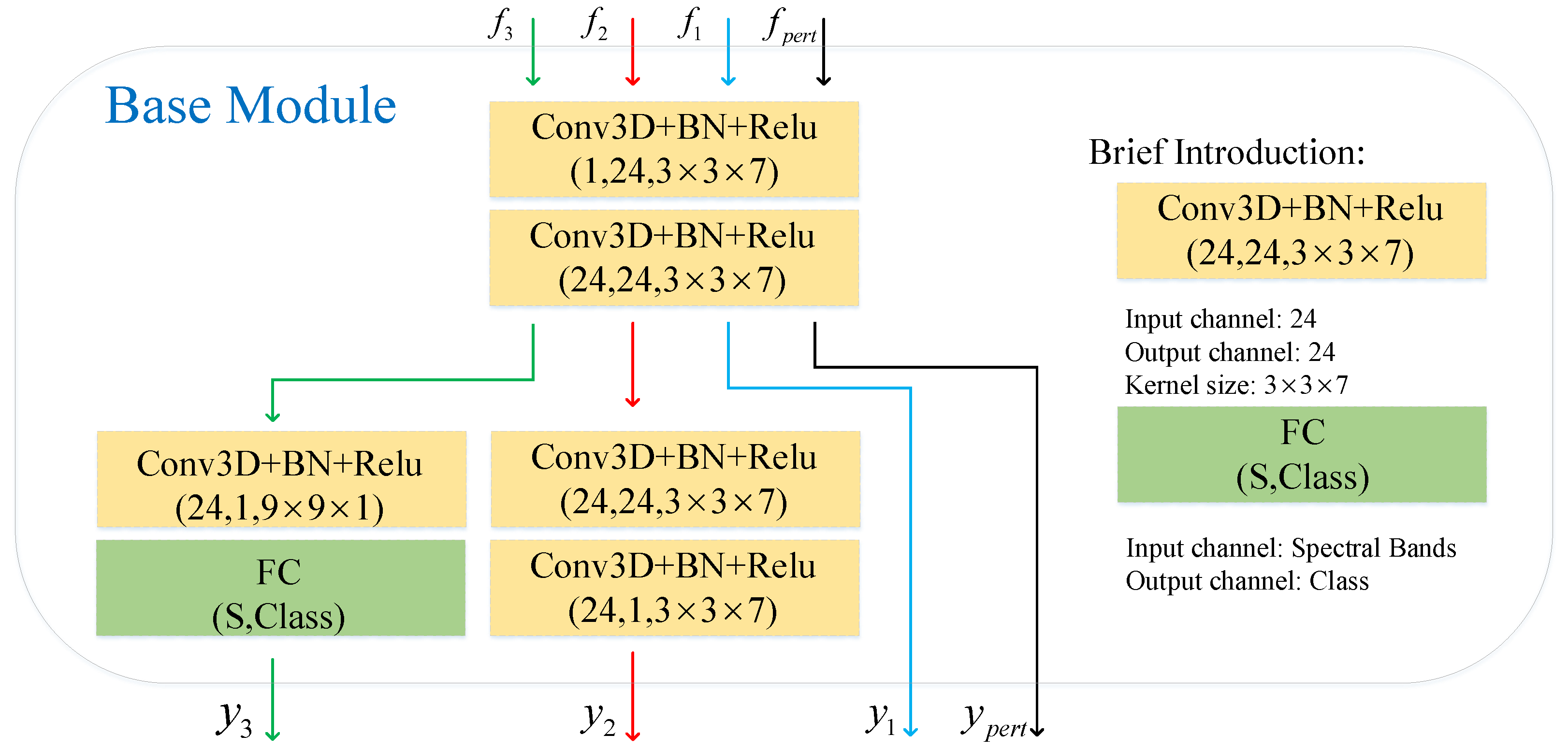
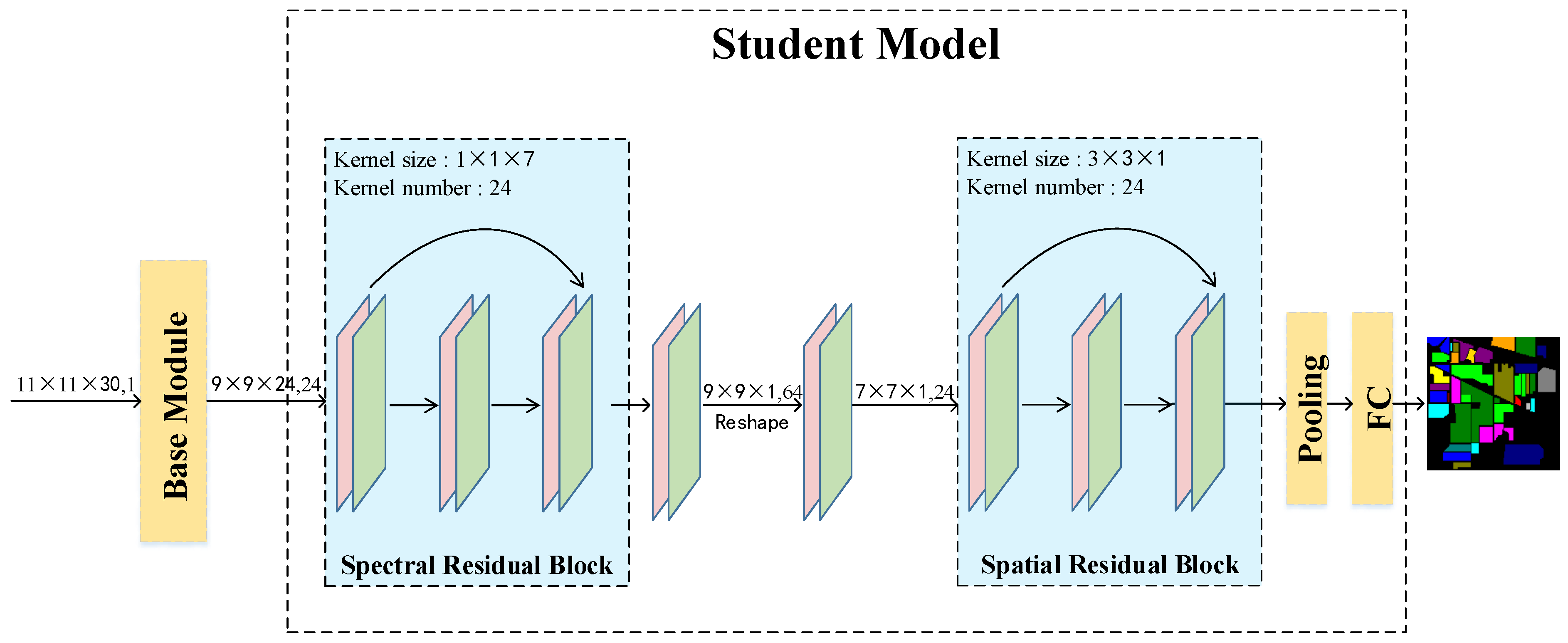
To verify our semi-supervised framework and better clarify our method, we design a residual network (RNet). The RNet is shown in Figure 2. The RNet comprises two modules: a BM and a residual feature extraction module (REM). The BM copes with the input feature α and outputs feature α shared by the following REM. The details of the BM are shown in Figure 3. The REM copes with the input feature α and outputs feature ϕ . Finally, ϕ is sent into the classifier for HSI classification.
The classical CNN model has been applied to hyperspectral classification and has achieved advanced results. However, the classification precision diminishes with the increase in the convolution layers [32]. This problem can be successfully eased by attaching shortcut connections between other layers to make residual blocks [33]. According to the spatial correlation and spectral characteristics of HSI, we designed a residual feature extraction module (REM). The residual structure is shown in Figure 2. We created two kinds of residual feature extraction modules: spectral residual and spatial residual modules. For the spectral residual feature extraction module, the size of the input feature is p × p × k and has n channels. The kernel size of 1 × 1 × d is applied to the two convolution layers. Meanwhile, the input feature is kept at p × p unaltered through a padding method. The spectral residual module is formulated as follows:
X i + 2 = X i + F ( X i ; θ )
where X i means the input feature of the i-th convolution layer, F X i ; θ represents the output feature of the ( i + 2 ) -th convolution layer, and θ is the weight parameter of the convolution layers.

2.2.3. Data Random Perturbation

Random perturbation is proved to be effective for robust semi-supervised learning models [28,29,30,31,34]. The work in [29] adds Gaussian noise to intermediate feature maps of the mean-teacher framework. For HSI data, spatial and spectral information are both essential. We propose a primary data random perturbation in our work: spectral feature shift.
Spectral feature shift is the bidirectional movement of some randomly selected spectral segments along the horizontal and vertical dimensions on the feature maps, respectively. The schematic diagrams of the spectral feature shift are shown in Figure 1. Therefore, spectral feature shift can significantly boost the multifariousness of the input features and make the semi-supervised learning model more robust. First, we randomly select μ spectral bands. Then, μ / 2 spectral bands are bidirectionally offset in the horizontal spatial dimension, and the other μ / 2 spectral bands are bidirectionally offset in the vertical spatial dimension. We use μ to mean the rank of the spectral shift. Moreover, we will discuss the influence of μ size on HSI classification accuracy in Section 3.
Each mini-batch incorporates both labeled HSI data and unlabeled HSI data during the training process. Moreover, we take a dropout method to avoid overfitting. The dropout strategy is a simple and effective technique that prevents overfitting by discarding a certain percentage of units during the training process [35]. In the mean-teacher framework, the labeled samples are trained using supervised loss. Unlabeled samples have no ground truth labels, so their supervised loss is undefined. Consistency regularization utilizes unlabeled HSI data based on the assumption that the model should output similar forecasts when fed perturbed forms of the same input. The consistency loss is utilized to the labeled HSI data and unlabeled HSI data in the semi-supervised branch. Therefore, the total loss in the semi-supervised branch is:
L s u p e r v i s e d = 1 N c i = 1 N c y i log y i
L s p e c t r a l _ s h i f t = 1 N i = 1 N s t u ( x s i ) t e a ( x i ) 2
L s e m i = L s u p e r v i s e d + λ 1 L s p e c t r a l _ s h i f t
where y i means the label of i-th training sample and y i indicates the predictive label, N c denotes the training samples with labels in each mini-batch, and x s i means the i-th training sample of spectral feature shift and s t u x s i is the output of the student model. Here, x i represents the i-th training sample and t e a x i is the output of the teacher model. It should be noted that only the training samples of the student network will be perturbed by the spectral feature shift. The hyper-parameters λ 1 are set to 1. L s p e c t r a l _ s h i f t is consistency loss for spectral feature shift random perturbation, and L s p e c t r a l _ s h i f t is L 2 -loss. L s u p e r v i s e d is supervised loss for the labeled data, and L s u p e r v i s e d is typical cross entropy loss.

2.3. Self-Supervised Learning Branch

Motivated by recent advances in self-supervised learning of HSI classification [32,36,37,38,39], we hypothesize that the semi-supervised HSI classification method could significantly benefit from self-supervised learning strategies. Furthermore, based on this motivation, we propose two auxiliary tasks in the self-supervised branch: masked bands reconstruction and spectral order forecast.

2.3.1. Masked Bands Reconstruction

As shown in Figure 1, the critical thought of this self-supervised auxiliary task is to generate the feature f 2 by stochastically masking the HSI feature f 1 at a few areas on the spatial dimensions. Then the BM utilizes f 2 to reconstruct f 1 . The schematic diagrams of the BM are shown in Figure 3. Masked bands reconstruction generates self-supervised signs from the original HSI feature f 1 , which could learn discriminative representations simply and effectively. The loss formula for the masked features auxiliary reconstruction task is:
L m a s k e d _ r e c o n s = 1 N i N m ( x i ) y r i 2
where m ( x i ) represents the i-th training sample of randomly masking the feature at some area along the spatial dimension, y r i means the reconstruction of the i-th training sample, and N represents the number of mini-batches.
At the same time, the SSRNet is trained in a multi-task pattern.In the pretext task of reconstruction of masked bands, the BM will be driven to notice and aggregate features from the context to predict the discarded areas. In this way, the learned features spontaneously conduct semi-supervised HSI classification. We use κ to mean the rank of the mask. Moreover, we will discuss the influence of κ size on HSI classification accuracy in Section 3.

2.3.2. Spectral Order Forecast

As shown in Figure 1, this auxiliary task needs to predict spectral feature sequences corrected in stochastically scrambled feature maps. The spectral order forecast is formulated as a classification task. The input is an HSI patch of clip spectral order, and the output is a probability distribution of the spectral order. The loss presentation for the spectral order forecast auxiliary task is:
L s p e c t r a l _ o r d e r = 1 N i = 1 N s i log s i
where s i means the i-th sample label for the correct spectral order, s i represents the i-th sample label for the predicted spectral order. Spectral order forecast can utilize the spectral order of features to learn discriminative spectral representations.

2.4. Overall Loss

The overall loss is made up of the losses from Section 2.2 and Section 2.3 The total loss function is:
L t o t a l = L s e m i + λ 2 L m a s k e d _ r e c o n s + λ 3 L s p e c t r a l _ o r d e r
Loss function L m a s k e d _ r e c o n s is designed for masked bands reconstruction, and L m a s k e d _ r e c o n s is L 2 -loss, while L s p e c t r a l _ o r d e r is cross entropy loss. Finally, the total loss function L t o t a l is made up of the L s e m i , L m a s k e d _ r e c o n s and the L s p e c t r a l _ o r d e r . Hyper-parameters λ 2 and λ 3 are set to 0.0001 and 0.001. A multi-task framework is exploited for optimization.

3. Experiments

In this section, we describe the experiment we performed to demonstrate the effectiveness of the proposed SSRNet for HSI classification. First, a brief introduction of the datasets used in the experiment is given, and then the experimental setup and comparison with other advanced methods follow. Lastly, we analyze the running time of the SSRNet and perform an ablation study to affirm the effectiveness of each component.

3.1. Dataset Description

Four widely used HSI datasets were used in the experiments, including Indian Pines, University of Pavia (PaviaU), Salinas and Houston 2013 datasets. We will give a short introduction of datasets as follows:
(1) Indian Pines: The dataset was collected by Airborne Visible/Infrared Imaging Spectrometer (AVIRIS) sensor over Northwestern Indiana. The data contain 200 spectral bands in the wavelength within range of 0.4 μ m to 2.5 μ m and 16 land cover categories. The spatial size is 145 × 145 pixels with resolution of 20 m/pixel. The total number of valid samples is 10,249 excluding background samples.
(2) University of Pavia: The dataset was captured by the ROSIS-03 sensor in the University of Pavia, Italy. The dataset consists of 103 spectral bands with the wavelength range of 0.43 μ m to 0.86 μ m and nine land cover classes, and its spatial size is 610 × 340 pixels, with a total of 42,776 labeled samples excluding background classes.
(3) Salinas: The dataset was collected by the AVIRIS sensor over Salinas Valley, California, USA. and consists of 204 spectral bands in the wavelength range of 0.4 μ m to 2.5 μ m and 16 land cover classes. The spatial size is 512 × 217 with the spatial resolution is 3.7 m/pixel. The total number of valid samples is 54,129, excluding background classes.
(4) Houston 2013: The dataset was acquired by the ITRES CASI-1500 sensor at the Houston University campus and its surrounding area, which contains 144 spectral bands in the wavelength range of 0.38 μ m to 1.05 μ m and 15 land cover classes, and its spatial size is 349 × 1905 , with a total of 15,029 labeled samples, excluding background classes. The spatial resolution is 2.5 m/pixel.

3.2. Experiment Setup

To assess the effectiveness of the SSRNet, we contrasted the SSRNet with other advanced HSI classification methods, including the traditional feature extraction method, SVM with RBF kernel [7], and other deep-learning-based classifiers: SSRN [40], SSLSTM [41], DBMA [42], HybridSN [43], CDCNN [44] and 3D-CAE [37]. Our proposed SSRNet and all DL-based methods were executed with PyTorch, and SVM was executed with sklearn. To make full utilization of unlabeled samples to improve learning performance, we randomly selected 10 labeled samples and 20% unlabeled samples for each class as training samples, and the rest as testing samples. For other supervised methods, we selected 10 labeled samples for each class as training samples. Details of training samples and testing samples of the dataset are listed in Table 1, Table 2, Table 3 and Table 4. The batch size was 16, the optimizer was Adam [45] with a learning rate of 0.0005, and the number of epochs was 80. Moreover, all experimTents at the same computing platform were configured with NVIDIA GeForce GTX1660 SUPER GPU and with 8 GB of memory. Next, the above methods will be briefly introduced.
(1) SVM [7] is a traditional classification method, and all spectral bands are taken as the input of the SVM with a radial basis function (RBF) kernel.
(2) SSRN [40] is a fully supervised method based on ResNet and 3D CNN in which the patch size is set to be 7 × 7 .
(3) SSLSTM [41] is a method using spectral–spatial long short-term memory (LSTM) networks.
(4) DBMA [42] is a supervised method based on a 3D CNN, attention mechanism and DenseNet in which the patch size is set to be 7 × 7 .
(5) HybridSN [43] is a supervised method of mixing a 3D CNN and a 2D CNN in which the patch size is set to be 25 × 25 .
(6) CDCNN [44] is a supervised method based on a 2D CNN and ResNet in which the patch size is set to be 5 × 5 .
(7) 3D-CAE [37] is a self-supervised method based on a 3D convolutional autoencoder in which the patch size is set to be 5 × 5 .

3.3. Experimental Results

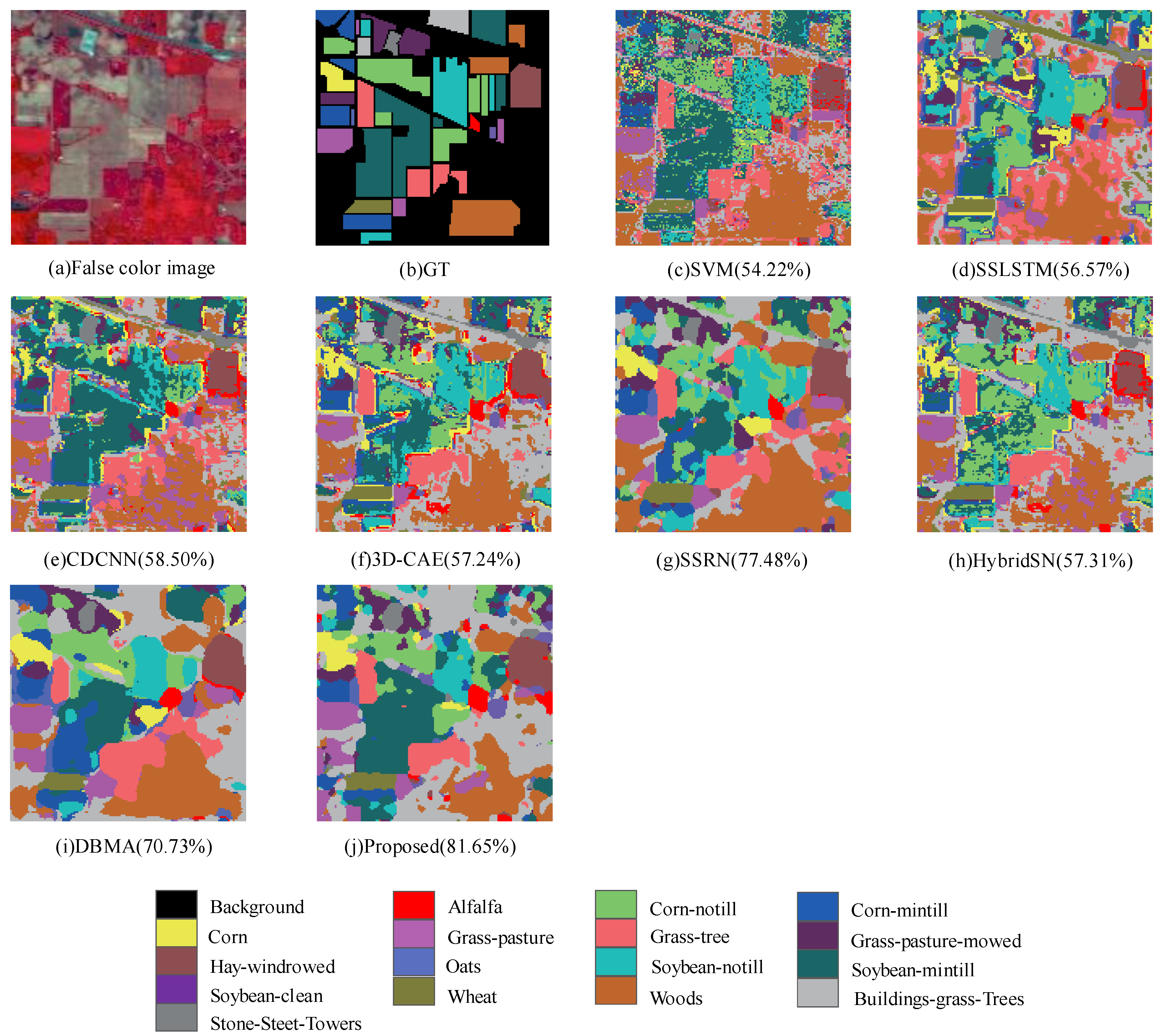
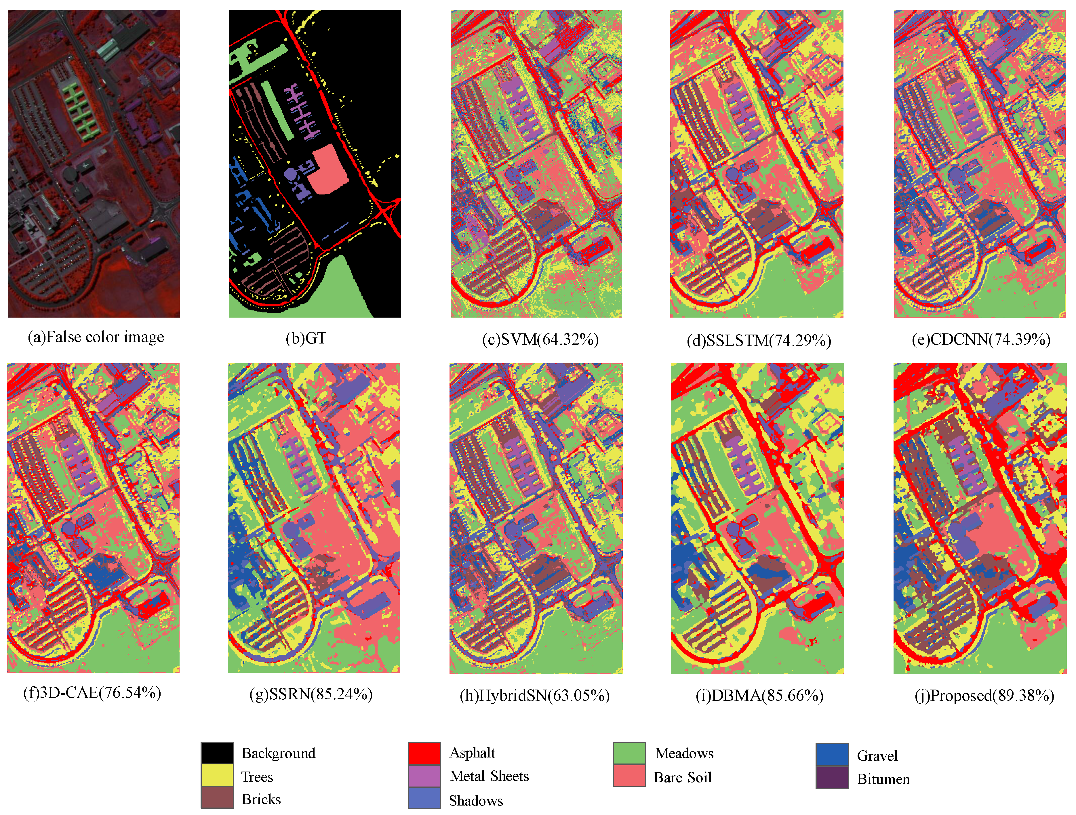
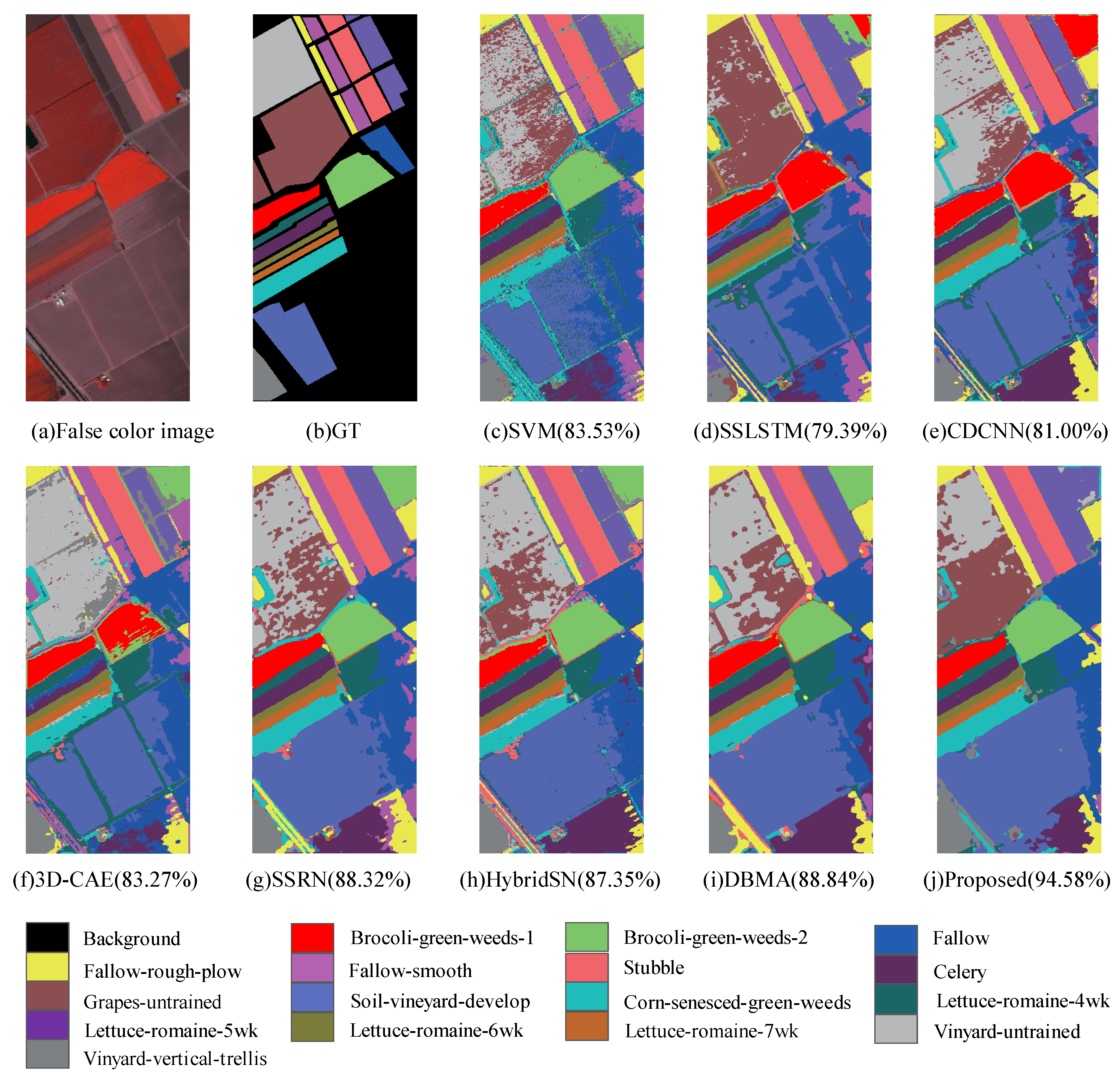
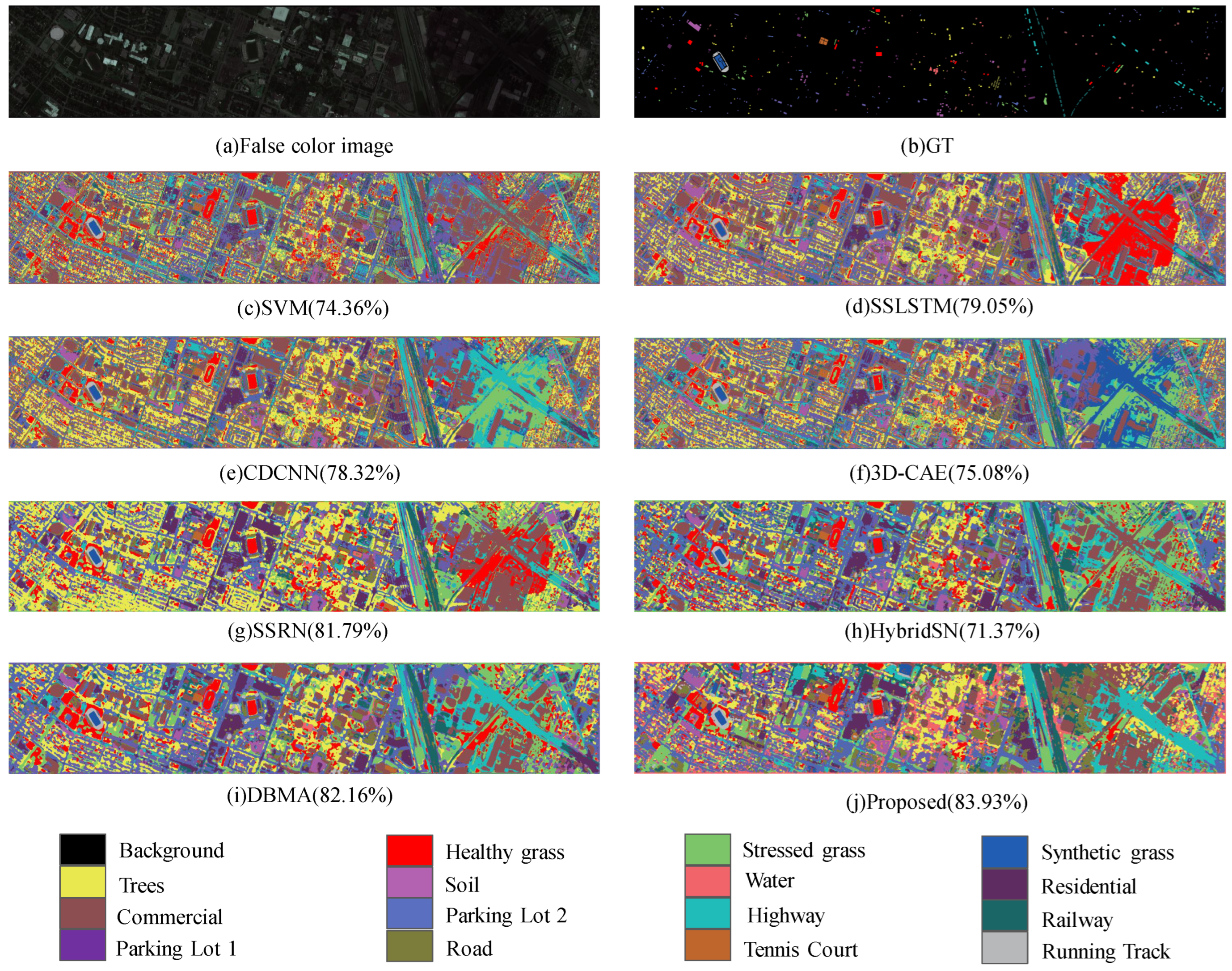
The results of overall accuracy (OA), average accuracy (AA), and Kappa coefficient (Kappa) are demonstrated in Table 5, Table 6, Table 7 and Table 8. Each experiment was repeated 10 times in which the mean and the standard deviation of each index were reported. Figure 4, Figure 5, Figure 6 and Figure 7 illustrates the classification maps of our SSRNet and other compared methods. The proposed methods outperform the compared methods on four datasets.
For instance, in the Indian Pines dataset, the SSRNet achieved the best OA of 81.65%, our SSRNet yielded over 20% higher than SVM (54.22%) and CDCNN (58.50%), and over 4% higher than other advanced deep-learning-based methods SSRN (77.48%) and DBMA (70.73%). In the University of Pavia, our proposed SSRNet was over 20% higher than the traditional SVM (64.32%), which was higher than the counterpart of SSRN (85.24%), CDCNN (74.39%) and DBMA (85.66%). Especially in the Salinas dataset, the SSRNet achieved the best OA of 93.47%, over 4% higher than advanced DBMA, but the OA of the other methods did not reach above 90%. Compared with self-supervised methods, the SSRNet was superior to the 3D-CAE in all four datasets, especially in the Indian Pines dataset, where the OA of SSRNet yielded over 20% higher than the 3D-CAE. We also made a visual comparison utilizing classification maps obtained by those methods. Other methods have classification errors in almost every land cover, and SSLSTM, CDCNN and 3D-CAE have obvious classification errors in the class of Broccoli-green-weeds-2 in the Salinas dataset. It can be observed that the SSRNet restored the distribution of surface objects well and maintained the best boundary region for these four datasets, which further validates the outstanding performance of the SSRNet.

3.4. Ablation Study

3.4.1. Complementarity between Components

The proposed SSRNet consists of two branches: semi-supervised and self-supervised. Spectral feature shift (S) proposes a random data perturbation strategy in the semi-supervised branch. Two auxiliary tasks are proposed in the self-supervised branch: masked bands reconstruction (R) and spectral order forecast (O). To prove the validity of our proposed three components, we made exhaustive ablation studies to evaluate different components of the SSRNet on the Indian Pines dataset and the Houston 2013 dataset. Ablation studies include the following:
  • SSRNet-S-R-O: The spectral feature shift in the semi-supervised branch is discarded, and two self-supervised auxiliary tasks are discarded;
  • SSRNet-S: Only the spectral feature shift in the semi-supervised branch is discarded;
  • SSRNet-R: Only the masked bands reconstruction in the self-supervised branch is discarded;
  • SSRNet-O: Only the spectral order forecast in the self-supervised branch is discarded;
  • SSRNet (ALL): No components are discarded.
We designed two data selection methods, one was 20% unlabeled samples and 10 labeled samples for each class, and the other was 20% unlabeled samples and 20 labeled samples for each class. Table 9 demonstrates that the three components are complementary. Moreover, perfect precision is achieved when integrated with three components (i.e., SSRNet (ALL)).

3.4.2. Choice of Hyper-Parameters

Figure 8 shows the OA of the spectral feature shift perturbation and the masked bands reconstruction auxiliary task under different hyper-parameter choices on the Indian Pines dataset in which the coefficient μ is used to denote the level of spectral feature shift, and the coefficient κ was used to mean the rank of mask. The adjustment of hyper-parameter has a certain effect of HSI classification precision. Moreover, μ = 6 and κ = 7 seem to be the best parameters.

3.4.3. Choice of Patch Size

Table 10 shows the OA of the SSRNet with various patch sizes, which varied from 7 × 7 to 13 × 13 with an interval of 2. As the patch size increased, the OA of the Salinas dataset kept increasing. For the other three datasets, the OA began to decline after 11 × 11, where they reached the highest OA of 83.96%, 90.99% and 85.54%, respectively. It has been found that the 11 × 11 patch size is most suitable.

3.5. Investigation on Running Time

The whole training time and testing time of our SSRNet and other methods are reported in Table 11, Table 12, Table 13 and Table 14. The SVM consumed less training and testing time than the deep-learning-based methods because the deep-learning-based methods have more parameters and larger input feature maps generally. Moreover, since our proposed SSRNet aims to improve learning performance by using fewer labeled samples and a large number of unlabeled samples, it requires more training time, but testing time still has one advantage compared with other methods. Considering the classification accuracy, our proposed SSRNet is competitive.
4. Conclusions

This paper incorporates self-supervised learning in the semi-supervised HSI classification and proposes a unified multi-task SSRNet framework. Especially in the semi-supervised branch, we have designed one type of random data perturbation and a residual feature extraction network to capture the spectral–spatial feature of HSI. We also presented two types of self-supervised auxiliary tasks for the SSRNet. The experiment results demonstrated that the SSRNet performs consistently with satisfactory performance for all four HSI datasets, especially when training samples are limited. As many unlabeled samples are utilized to improve learning performance, we will explore how to decrease training time in future work.

Author Contributions

Conceptualization, L.S. and Z.F.; methodology, L.S.; software, L.S.; validation, L.S., Z.F. and X.Z.; formal analysis, L.S.; investigation, L.S.; resources, S.Y.; data curation, X.Z.; writing—original draft preparation, L.S.; writing—review and editing, S.Y., Z.F. and L.J.; visualization, L.S. and X.Z.; supervision, S.Y.; project administration, S.Y.; funding acquisition, S.Y. All authors have read and agreed to the published version of the manuscript.

Funding

This work was supported by the National Natural Science Foundation of China (Nos. 61906145, 61771376, 61771380); the Science and Technology Innovation Team in Shaanxi Province of China (Nos. 2020TD-017); the 111 Project, the Foundation of Key Laboratory of Aerospace Science and Industry Group of CASIC, China; the Key Project of Hubei Provincial Natural Science Foundation under Grant 2020CFA001, China.

Data Availability Statement

The Indiana Pines, University of Pavia, and Salinas Valley datasets are available online at https://www.ehu.eus/ccwintco/index.php?title=Hyperspectral_Remote_Sensing_Scenes (accessed on 3 July 2021). The Houston 2013 dataset is available online at https://hyperspectral.ee.uh.edu/?page_id=459 (accessed on 3 July 2021).

Conflicts of Interest

The authors declare no conflict of interest.

References

  1. Li, Z.; Huang, L.; He, J. A multiscale deep middle-level feature fusion network for hyperspectral classification. Remote Sens. 2019, 11, 695. [Google Scholar] [CrossRef] [Green Version]
  2. Awad, M.; Jomaa, I.; Arab, F. Improved capability in stone pine forest mapping and management in Lebanon using hyperspectral CHRIS-Proba data relative to Landsat ETM+. Photogramm. Eng. Remote Sens. 2014, 80, 725–731. [Google Scholar] [CrossRef]
  3. Ibrahim, A.; Franz, B.; Ahmad, Z.; Healy, R.; Knobelspiesse, K.; Gao, B.C.; Proctor, C.; Zhai, P.W. Atmospheric correction for hyperspectral ocean color retrieval with application to the Hyperspectral Imager for the Coastal Ocean (HICO). Remote Sens. Environ. 2018, 204, 60–75. [Google Scholar] [CrossRef] [Green Version]
  4. Foglini, F.; Angeletti, L.; Bracchi, V.; Chimienti, G.; Grande, V.; Hansen, I.M.; Meroni, A.N.; Marchese, F.; Mercorella, A.; Prampolini, M.; et al. Underwater Hyperspectral Imaging for seafloor and benthic habitat mapping. In Proceedings of the 2018 IEEE International Workshop on Metrology for the Sea; Learning to Measure Sea Health Parameters (MetroSea), Bari, Italy, 8–10 October 2018; pp. 201–205. [Google Scholar]
  5. Ghamisi, P.; Yokoya, N.; Li, J.; Liao, W.; Liu, S.; Plaza, J.; Rasti, B.; Plaza, A. Advances in hyperspectral image and signal processing: A comprehensive overview of the state of the art. IEEE Geosci. Remote Sens. Mag. 2017, 5, 37–78. [Google Scholar] [CrossRef] [Green Version]
  6. Villa, A.; Benediktsson, J.A.; Chanussot, J.; Jutten, C. Hyperspectral image classification with independent component discriminant analysis. IEEE Trans. Geosci. Remote Sens. 2011, 49, 4865–4876. [Google Scholar] [CrossRef] [Green Version]
  7. Melgani, F.; Bruzzone, L. Classification of hyperspectral remote sensing images with support vector machines. IEEE Trans. Geosci. Remote Sens. 2004, 42, 1778–1790. [Google Scholar] [CrossRef] [Green Version]
  8. Ghamisi, P.; Maggiori, E.; Li, S.; Souza, R.; Tarablaka, Y.; Moser, G.; De Giorgi, A.; Fang, L.; Chen, Y.; Chi, M.; et al. New frontiers in spectral–spatial hyperspectral image classification: The latest advances based on mathematical morphology, Markov random fields, segmentation, sparse representation, and deep learning. IEEE Geosci. Remote Sens. Mag. 2018, 6, 10–43. [Google Scholar] [CrossRef]
  9. Benediktsson, J.A.; Palmason, J.A.; Sveinsson, J.R. Classification of hyperspectral data from urban areas based on extended morphological profiles. IEEE Trans. Geosci. Remote Sens. 2005, 43, 480–491. [Google Scholar] [CrossRef]
  10. Krizhevsky, A.; Sutskever, I.; Hinton, G.E. Imagenet classification with deep convolutional neural networks. Adv. Neural Inf. Process. Syst. 2012, 25. [Google Scholar] [CrossRef]
  11. Makantasis, K.; Karantzalos, K.; Doulamis, A.; Doulamis, N. Deep supervised learning for hyperspectral data classification through convolutional neural networks. In Proceedings of the 2015 IEEE International Geoscience and Remote Sensing Symposium (IGARSS), Milan, Italy, 26–31 July 2015; pp. 4959–4962. [Google Scholar]
  12. Hu, W.; Huang, Y.; Wei, L.; Zhang, F.; Li, H. Deep convolutional neural networks for hyperspectral image classification. J. Sens. 2015, 2015, 12. [Google Scholar] [CrossRef] [Green Version]
  13. Chen, Y.; Jiang, H.; Li, C.; Jia, X.; Ghamisi, P. Deep feature extraction and classification of hyperspectral images based on convolutional neural networks. IEEE Trans. Geosci. Remote Sens. 2016, 54, 6232–6251. [Google Scholar] [CrossRef] [Green Version]
  14. Cheng, C.; Li, H.; Peng, J.; Cui, W.; Zhang, L. Hyperspectral image classification via spectral–spatial random patches network. IEEE J. Sel. Top. Appl. Earth Obs. Remote Sens. 2021, 14, 4753–4764. [Google Scholar] [CrossRef]
  15. Dópido, I.; Li, J.; Marpu, P.R.; Plaza, A.; Dias, J.M.B.; Benediktsson, J.A. Semisupervised self-learning for hyperspectral image classification. IEEE Trans. Geosci. Remote Sens. 2013, 51, 4032–4044. [Google Scholar] [CrossRef] [Green Version]
  16. Li, F.; Clausi, D.A.; Xu, L.; Wong, A. ST-IRGS: A region-based self-training algorithm applied to hyperspectral image classification and segmentation. IEEE Trans. Geosci. Remote Sens. 2017, 56, 3–16. [Google Scholar] [CrossRef]
  17. Wu, Y.; Mu, G.; Qin, C.; Miao, Q.; Ma, W.; Zhang, X. Semi-supervised hyperspectral image classification via spatial-regulated self-training. Remote Sens. 2020, 12, 159. [Google Scholar] [CrossRef] [Green Version]
  18. He, Z.; Liu, H.; Wang, Y.; Hu, J. Generative adversarial networks-based semi-supervised learning for hyperspectral image classification. Remote Sens. 2017, 9, 1042. [Google Scholar] [CrossRef] [Green Version]
  19. Feng, J.; Ye, Z.; Li, D.; Liang, Y.; Tang, X.; Zhang, X. Hyperspectral Image Classification Based on Semi-Supervised Dual-Branch Convolutional Autoencoder with Self-Attention. In Proceedings of the IGARSS 2020-2020 IEEE International Geoscience and Remote Sensing Symposium, Waikoloa, HI, USA, 26 September–2 October 2020; pp. 1267–1270. [Google Scholar]
  20. Li, J.; Bioucas-Dias, J.M.; Plaza, A. Semisupervised hyperspectral image classification using soft sparse multinomial logistic regression. IEEE Geosci. Remote Sens. Lett. 2012, 10, 318–322. [Google Scholar]
  21. Camps-Valls, G.; Marsheva, T.V.B.; Zhou, D. Semi-supervised graph-based hyperspectral image classification. IEEE Trans. Geosci. Remote Sens. 2007, 45, 3044–3054. [Google Scholar] [CrossRef]
  22. De Morsier, F.; Borgeaud, M.; Gass, V.; Thiran, J.P.; Tuia, D. Kernel low-rank and sparse graph for unsupervised and semi-supervised classification of hyperspectral images. IEEE Trans. Geosci. Remote Sens. 2016, 54, 3410–3420. [Google Scholar] [CrossRef]
  23. Ding, Y.; Zhao, X.; Zhang, Z.; Cai, W.; Yang, N.; Zhan, Y. Semi-supervised locality preserving dense graph neural network with ARMA filters and context-aware learning for hyperspectral image classification. IEEE Trans. Geosci. Remote Sens. 2021, 60, 1–12. [Google Scholar] [CrossRef]
  24. Sun, Q.; Liu, X.; Bourennane, S. Unsupervised Multi-Level Feature Extraction for Improvement of Hyperspectral Classification. Remote Sens. 2021, 13, 1602. [Google Scholar] [CrossRef]
  25. Zhao, B.; Ulfarsson, M.O.; Sveinsson, J.R.; Chanussot, J. Unsupervised and supervised feature extraction methods for hyperspectral images based on mixtures of factor analyzers. Remote Sens. 2020, 12, 1179. [Google Scholar] [CrossRef] [Green Version]
  26. Zhu, M.; Fan, J.; Yang, Q.; Chen, T. SC-EADNet: A Self-supervised Contrastive Efficient Asymmetric Dilated Network for Hyperspectral Image Classification. IEEE Trans. Geosci. Remote Sens. 2021, 60, 1–17. [Google Scholar] [CrossRef]
  27. Yue, J.; Fang, L.; Rahmani, H.; Ghamisi, P. Self-supervised learning with adaptive distillation for hyperspectral image classification. IEEE Trans. Geosci. Remote Sens. 2021, 60, 1–13. [Google Scholar] [CrossRef]
  28. Miyato, T.; Maeda, S.i.; Koyama, M.; Ishii, S. Virtual adversarial training: A regularization method for supervised and semi-supervised learning. IEEE Trans. Pattern Anal. Mach. Intell. 2018, 41, 1979–1993. [Google Scholar] [CrossRef] [PubMed] [Green Version]
  29. Tarvainen, A.; Valpola, H. Mean-teachers are better role models: Weight-averaged consistency targets improve semi-supervised deep learning results. Adv. Neural Inf. Process. Syst. 2017, 30, 1195–1204. [Google Scholar]
  30. Wang, X.; Kihara, D.; Luo, J.; Qi, G.J. Enaet: Self-trained ensemble autoencoding transformations for semi-supervised learning. arXiv 2019, arXiv:1911.09265. [Google Scholar]
  31. Berthelot, D.; Carlini, N.; Goodfellow, I.; Papernot, N.; Oliver, A.; Raffel, C.A. Mixmatch: A holistic approach to semi-supervised learning. Adv. Neural Inf. Process. Syst. 2019, 32, 5050–5060. [Google Scholar]
  32. Chen, Y.; Lin, Z.; Zhao, X.; Wang, G.; Gu, Y. Deep learning-based classification of hyperspectral data. IEEE J. Sel. Top. Appl. Earth Obs. Remote Sens. 2014, 7, 2094–2107. [Google Scholar] [CrossRef]
  33. He, K.; Zhang, X.; Ren, S.; Sun, J. Deep residual learning for image recognition. In Proceedings of the IEEE Conference on Computer Vision and Pattern Recognition, Las Vegas, NV, USA, 27–30 June 2016; pp. 770–778. [Google Scholar]
  34. Laine, S.; Aila, T. Temporal ensembling for semi-supervised learning. arXiv 2016, arXiv:1610.02242. [Google Scholar]
  35. Srivastava, N.; Hinton, G.; Krizhevsky, A.; Sutskever, I.; Salakhutdinov, R. Dropout: A simple way to prevent neural networks from overfitting. J. Mach. Learn. Res. 2014, 15, 1929–1958. [Google Scholar]
  36. Tao, C.; Pan, H.; Li, Y.; Zou, Z. Unsupervised spectral–spatial feature learning with stacked sparse autoencoder for hyperspectral imagery classification. IEEE Geosci. Remote Sens. Lett. 2015, 12, 2438–2442. [Google Scholar]
  37. Mei, S.; Ji, J.; Geng, Y.; Zhang, Z.; Li, X.; Du, Q. Unsupervised spatial–spectral feature learning by 3D convolutional autoencoder for hyperspectral classification. IEEE Trans. Geosci. Remote Sens. 2019, 57, 6808–6820. [Google Scholar] [CrossRef]
  38. Liu, L.; Wang, Y.; Peng, J.; Zhang, L.; Zhang, B.; Cao, Y. Latent relationship guided stacked sparse autoencoder for hyperspectral imagery classification. IEEE Trans. Geosci. Remote Sens. 2020, 58, 3711–3725. [Google Scholar] [CrossRef]
  39. Liu, B.; Yu, A.; Yu, X.; Wang, R.; Gao, K.; Guo, W. Deep multiview learning for hyperspectral image classification. IEEE Trans. Geosci. Remote Sens. 2020, 59, 7758–7772. [Google Scholar] [CrossRef]
  40. Zhong, Z.; Li, J.; Luo, Z.; Chapman, M. Spectral–spatial residual network for hyperspectral image classification: A 3-D deep learning framework. IEEE Trans. Geosci. Remote Sens. 2017, 56, 847–858. [Google Scholar] [CrossRef]
  41. Zhou, F.; Hang, R.; Liu, Q.; Yuan, X. Hyperspectral image classification using spectral–spatial LSTMs. Neurocomputing 2019, 328, 39–47. [Google Scholar] [CrossRef]
  42. Ma, W.; Yang, Q.; Wu, Y.; Zhao, W.; Zhang, X. Double-branch multi-attention mechanism network for hyperspectral image classification. Remote Sens. 2019, 11, 1307. [Google Scholar] [CrossRef] [Green Version]
  43. Roy, S.K.; Krishna, G.; Dubey, S.R.; Chaudhuri, B.B. HybridSN: Exploring 3-D–2-D CNN feature hierarchy for hyperspectral image classification. IEEE Geosci. Remote Sens. Lett. 2019, 17, 277–281. [Google Scholar] [CrossRef] [Green Version]
  44. Lee, H.; Kwon, H. Going deeper with contextual CNN for hyperspectral image classification. IEEE Trans. Image Process. 2017, 26, 4843–4855. [Google Scholar] [CrossRef] [Green Version]
  45. Kingma, D.P.; Ba, J. Adam: A method for stochastic optimization. arXiv 2014, arXiv:1412.6980. [Google Scholar]
Figure 1. Overview of the proposed SSRNet.
Remotesensing 14 02997 g001
Figure 2. The details structure of the RNet.
Remotesensing 14 02997 g002
Figure 3. The details structure of the base module.
Remotesensing 14 02997 g003
Figure 4. The classification maps of the Indian Pines with 10 labeled samples.
Remotesensing 14 02997 g004
Figure 5. The classification maps of the University of Pavia with 10 labeled samples.
Remotesensing 14 02997 g005
Figure 6. The classification maps of the Salinas with 10 labeled samples.
Remotesensing 14 02997 g006
Figure 7. The classification maps of the Houston 2013 with 10 labeled samples.
Remotesensing 14 02997 g007
Figure 8. The effects of spectral feature shift and masked bands reconstruction auxiliary task under different hyper-parameter choices on the Indian Pines dataset.
Remotesensing 14 02997 g008
Table 1. The number of training, testing samples in the Indian Pines dataset.
Class No.Land Cover TypeTrainingTesting
1Alfalfa1027
2Corn-notill101133
3Corn-mintill10655
4Corn10180
5Grass-pasture10377
6Grass-tree10575
7Grass-pasture-mowed1013
8Hay-windrowed10373
9Oats107
10Soybean-notill10768
11Soybean-mintill101955
12Soybean-clean10465
13Wheat10155
14Woods101003
15Buildings-Grass-Trees10299
16Stone-Steel-Towers1065
Total1608050
Table 2. The number of training, testing samples in the University of Pavia dataset.
Class No.Land Cover TypeTrainingTesting
1Asphalt105295
2Meadows1014,910
3Gravel101670
4Trees102442
5Metal Sheets101067
6Bare Soil104014
7Bitumen101055
8Bricks102936
9Shadows10748
Total9034,137
Table 3. The number of training, testing samples in the Salinas dataset.
Class No.Land Cover TypeTrainingTesting
1Brocoli-green-weeds-1101598
2Brocoli-green-weeds-2102971
3Fallow101571
4Fallow-rough-plow101106
5Fallow-smooth102133
6Stubble103158
7Celery102854
8Grapes-untrained109007
9Soil-vinyard-develop109007
10Corn-senesced-green-weeds104953
11Lettuce-romaine-4wk102613
12Lettuce-romaine-5wk10845
13Lettuce-romaine-6wk101532
14Lettuce-romaine-7wk10723
15Vinyard-untrained10847
16Vinyard-vertical-trellis105805
Total16043,152
Table 4. The number of training and testing samples in the Houston 2013 dataset.
Class No.Land Cover TypeTrainingTesting
1Healthy grass10991
2Stressed grass10994
3Synthetic grass10548
4Trees10986
5Soil10984
6Water10251
7Residential101005
8Commercial10986
9Road10992
10Highway10972
11Railway10979
12Parking Lot 110977
13Parking Lot 210366
14Tennis Court10333
15Running Track10519
Total15011,883
Table 5. Classification results on the Indian Pines dataset with 10 labeled samples, including OA (%), AA (%) and Kappa×100 in which the best results are denoted in bold.
Class No.SVM [7]SSLSTM [41]CDCNN [44]3DCAE [37]SSRN [40]HybridSN [43]DBMA [42]Proposed
120.59 ± 4.5530.55 ± 10.835.84 ± 13.852.98 ± 28.971.49 ± 19.334.37 ± 25.674.96 ± 15.298.76 ± 1.74
242.21 ± 4.3155.35 ± 7.8955.86 ± 13.350.15 ± 19.476.25 ± 7.4758.12 ± 8.7465.09 ± 9.1166.66 ± 11.7
335.40 ± 10.037.91 ± 11.139.87 ± 8.6348.59 ± 14.169.08 ± 16.145.15 ± 15.057.39 ± 14.864.98 ± 7.70
423.26 ± 3.9637.88 ± 12.234.71 ± 9.8331.33 ± 10.657.53 ± 15.335.23 ± 15.754.05 ± 15.995.36 ± 4.72
563.52 ± 8.9464.48 ± 19.265.62 ± 15.578.46 ± 12.093.90 ± 7.1770.62 ± 18.092.35 ± 4.5585.76 ± 5.11
687.13 ± 2.9578.57 ± 10.985.22 ± 6.2272.74 ± 17.896.64 ± 3.5482.52 ± 10.997.43 ± 2.9798.60 ± 0.37
726.52 ± 12.418.81 ± 6.4123.40 ± 0.1135.70 ± 23.145.81 ± 21.927.74 ± 24.325.73 ± 9.42100.0 ± 0.00
895.51 ± 1.0895.07 ± 4.3096.42 ± 11.982.92 ± 28.198.63 ± 3.2277.09 ± 31.899.86 ± 0.2299.55 ± 0.63
913.41 ± 5.0614.39 ± 6.6917.52 ± 3.0920.37 ± 20.346.15 ± 18.920.35 ± 21.009.61 ± 4.89100.0 ± 0.00
1046.77 ± 7.5146.61 ± 7.8617.52 ± 11.649.53 ± 21.467.42 ± 12.357.34 ± 9.6167.32 ± 12.579.16 ± 3.40
1162.14 ± 4.6963.90 ± 6.0064.98 ± 10.164.19 ± 21.879.76 ± 6.1569.35 ± 9.0978.54 ± 8.2575.91 ± 4.42
1228.09 ± 2.8431.50 ± 6.7431.74 ± 7.2842.24 ± 17.159.93 ± 14.635.25 ± 14.652.58 ± 18.679.92 ± 3.78
1382.81 ± 5.2676.39 ± 8.1283.83 ± 7.0973.12 ± 19.394.87 ± 4.7877.85 ± 16.091.57 ± 8.6299.13 ± 1.22
1489.44 ± 4.2383.15 ± 6.2787.19 ± 11.086.55 ± 9.0897.12 ± 1.7586.37 ± 10.194.90 ± 4.4294.94 ± 0.44
1542.56 ± 6.7547.70 ± 9.2053.70 ± 4.0048.42 ± 17.275.73 ± 10.241.17 ± 9.8160.55 ± 9.6692.52 ± 5.06
1691.39 ± 8.2267.35 ± 11.668.15 ± 18.961.69 ± 12.384.12 ± 9.8150.83 ± 6.6881.72 ± 9.11100.0 ± 0.00
OA (%)54.22 ± 2.4756.57 ± 3.4958.50 ± 3.3657.24 ± 4.6677.48 ± 3.9657.31 ± 5.8370.73 ± 4.8381.65 ± 1.71
AA (%)55.09 ± 1.7453.10 ± 2.2555.89 ± 3.5356.19 ± 6.3775.90 ± 3.7154.34 ± 4.8768.98 ± 2.6786.46 ± 1.17
Kappa×10048.88 ± 2.6451.08 ± 3.6253.20 ± 3.5652.75 ± 4.7174.61 ± 4.2452.66 ± 6.0567.09 ± 5.2579.21 ± 1.92
Table 6. Classification results on the University of Pavia dataset with 10 labeled samples, including OA (%), AA (%) and Kappa×100 in which the best results are denoted in bold.
Class No.SVM [7]SSLSTM [41]CDCNN [44]3DCAE [37]SSRN [40]HybridSN [43]DBMA [42]Proposed
192.38 ± 2.0592.66 ± 1.6590.29 ± 3.1780.00 ± 13.198.18 ± 1.1654.58 ± 30.395.64 ± 2.0686.09 ± 9.03
281.67 ± 8.2588.39 ± 1.3092.00 ± 2.2893.54 ± 1.3296.29 ± 2.1373.87 ± 37.296.78 ± 2.4090.80 ± 2.75
340.65 ± 4.7252.57 ± 5.1151.01 ± 14.858.49 ± 5.7064.42 ± 11.934.77 ± 20.977.21 ± 12.191.01 ± 7.41
460.97 ± 11.870.93 ± 11.875.75 ± 16.166.91 ± 10.179.92 ± 16.960.83 ± 23.385.22 ± 18.093.51 ± 5.09
590.77 ± 6.9292.17 ± 3.9293.47 ± 5.7763.32 ± 44.899.10 ± 1.4894.49 ± 4.9698.86 ± 1.2199.75 ± 0.35
634.24 ± 5.0945.63 ± 6.3551.85 ± 16.178.07 ± 4.0473.38 ± 15.358.08 ± 19.765.15 ± 13.596.51 ± 3.04
744.62 ± 5.8450.90 ± 6.0552.51 ± 14.565.12 ± 11.966.81 ± 16.153.73 ± 17.885.52 ± 15.697.75 ± 1.51
870.31 ± 6.7379.22 ± 2.6473.13 ± 6.8049.34 ± 1.7079.65 ± 6.8146.58 ± 11.681.79 ± 7.1764.77 ± 31.3
999.88 ± 0.1099.89 ± 0.0961.63 ± 24.765.24 ± 19.599.55 ± 0.8657.31 ± 20.792.01 ± 4.2598.74 ± 1.24
OA (%)64.32 ± 6.2974.29 ± 2.7274.39 ± 6.5076.54 ± 4.6885.24 ± 4.3263.05 ± 12.585.66 ± 4.5589.38 ± 1.14
AA (%)68.39 ± 1.8574.71 ± 2.0871.29 ± 5.3668.89 ± 5.4984.14 ± 2.9059.36 ± 9.4286.46 ± 3.7490.99 ± 1.88
Kappa×10055.47 ± 6.6367.36 ± 3.1367.68 ± 7.6070.13 ± 5.4581.08 ± 5.2555.59 ± 12.481.72 ± 5.4986.18 ± 1.52
Table 7. Classification results on the Salinas dataset with 10 labeled samples, including OA (%), AA (%) and Kappa×100 in which the best results are denoted in bold.
Class No.SVM [7]SSLSTM [41]CDCNN [44]3DCAE [37]SSRN [40]HybridSN [43]DBMA [42]Proposed
198.49 ± 1.3781.94 ± 21.285.02 ± 20.281.68 ± 16.287.74 ± 30.095.46 ± 6.9999.10 ± 2.6899.70 ± 0.23
298.95 ± 0.4185.61 ± 15.496.29 ± 6.3789.38 ± 4.8599.96 ± 0.0794.02 ± 6.4399.99 ± 0.0297.76 ± 2.87
386.03 ± 5.2993.98 ± 4.9191.71 ± 8.0964.88 ± 45.892.56 ± 4.1995.29 ± 4.5897.60 ± 1.1099.95 ± 0.06
497.30 ± 1.0696.62 ± 2.3893.23 ± 8.5674.28 ± 23.992.98 ± 13.292.07 ± 8.1190.69 ± 2.5798.79 ± 1.28
597.14 ± 1.7099.09 ± 0.4896.47 ± 3.9493.84 ± 4.2898.47 ± 2.3293.55 ± 4.9998.75 ± 1.6497.24 ± 0.05
699.94 ± 0.0698.93 ± 0.6697.01 ± 2.1795.86 ± 1.9099.94 ± 0.0697.65 ± 3.4699.58 ± 0.5399.61 ± 0.47
795.38 ± 2.6598.67 ± 1.0597.25 ± 2.9194.80 ± 5.3596.50 ± 6.3597.62 ± 2.1797.85 ± 2.7199.45 ± 0.77
870.82 ± 2.5680.39 ± 7.4068.33 ± 21.780.99 ± 3.2382.33 ± 4.7583.57 ± 5.7889.42 ± 5.0084.84 ± 4.97
998.83 ± 1.1598.27 ± 1.5499.41 ± 0.4492.80 ± 1.8297.27 ± 6.3895.79 ± 4.6899.36 ± 0.4199.86 ± 0.16
1078.67 ± 9.3787.99 ± 1.9385.23 ± 5.8290.92 ± 6.5694.13 ± 4.2886.57 ± 10.290.55 ± 4.9789.34 ± 6.07
1179.57 ± 7.8581.93 ± 8.7972.03 ± 11.274.02 ± 13.695.38 ± 2.0283.11 ± 16.691.55 ± 7.8199.84 ± 0.22
1293.88 ± 3.6596.57 ± 1.3195.91 ± 3.2296.74 ± 2.8599.34 ± 0.6586.96 ± 29.199.40 ± 0.9598.86 ± 1.41
1391.47 ± 5.1992.15 ± 3.2288.81 ± 7.9254.86 ± 8.1896.05 ± 8.7433.20 ± 42.291.69 ± 6.8398.42 ± 1.43
1483.71 ± 9.7395.53 ± 3.4292.89 ± 4.4471.57 ± 8.5488.55 ± 22.853.57 ± 24.592.71 ± 7.9498.97 ± 0.54
1554.96 ± 5.7744.81 ± 3.0752.23 ± 7.0470.13 ± 14.766.87 ± 9.1278.20 ± 7.7564.27 ± 12.883.68 ± 3.80
1690.53 ± 5.7592.04 ± 9.0894.44 ± 3.9183.88 ± 7.2599.37 ± 0.8289.07 ± 9.2698.35 ± 1.9799.44 ± 0.46
OA (%)83.53 ± 1.8179.39 ± 2.8281.00 ± 3.9183.27 ± 5.7288.32 ± 5.7687.35 ± 3.3088.84 ± 4.0393.47 ± 1.04
AA (%)88.48 ± 1.2289.03 ± 2.7687.89 ± 2.3781.91 ± 6.8692.96 ± 5.1884.73 ± 6.4193.80 ± 1.3396.61 ± 0.05
Kappa×10081.73 ± 1.9777.31 ± 3.0978.97 ± 4.2481.52 ± 6.2587.03 ± 6.3585.97 ± 3.6487.67 ± 4.4092.75 ± 1.15
Table 8. Classification results on the Houston 2013 dataset with 10 labeled samples, including OA (%), AA (%) and Kappa×100 in which the best results are denoted in bold.
Class No.SVM [7]SSLSTM [41]CDCNN [44]3DCAE [37]SSRN [40]HybridSN [43]DBMA [42]Proposed
188.65 ± 4.3279.20 ± 10.881.77 ± 9.5087.56 ± 6.2583.84 ± 5.7875.18 ± 26.588.33 ± 4.2483.18 ± 4.24
291.38 ± 6.5494.13 ± 7.3589.77 ± 10.793.06 ± 3.6594.26 ± 5.2477.59 ± 12.492.36 ± 4.3387.58 ± 9.24
387.88 ± 11.275.87 ± 23.588.05 ± 15.787.45 ± 10.699.64 ± 0.4392.56 ± 6.9999.94 ± 0.1198.17 ± 2.06
496.09 ± 3.5391.05 ± 10.694.96 ± 5.6991.28 ± 3.3397.07 ± 2.2581.88 ± 12.094.66 ± 8.9991.74 ± 4.71
590.91 ± 2.6292.36 ± 2.7195.36 ± 2.7588.39 ± 2.5193.15 ± 4.8384.62 ± 8.5893.91 ± 3.1199.96 ± 0.05
693.99 ± 5.8895.70 ± 3.3185.34 ± 6.9793.55 ± 5.9594.97 ± 8.8879.39 ± 18.995.22 ± 3.2699.46 ± 0.75
767.72 ± 9.4079.74 ± 7.1474.40 ± 4.4270.47 ± 14.375.90 ± 10.163.50 ± 13.078.17 ± 12.675.28 ± 2.72
866.75 ± 10.984.54 ± 4.3381.29 ± 9.6756.72 ± 5.7280.49 ± 21.449.88 ± 30.894.07 ± 6.1264.56 ± 13.0
962.88 ± 9.7472.80 ± 7.1870.61 ± 9.8361.88 ± 14.966.63 ± 7.9364.06 ± 12.375.42 ± 8.3170.46 ± 7.82
1059.57 ± 7.4967.72 ± 9.7161.68 ± 9.1939.36 ± 28.269.39 ± 12.357.21 ± 24.770.02 ± 10.778.22 ± 4.01
1158.80 ± 6.8364.71 ± 7.7165.33 ± 9.4483.24 ± 3.7977.09 ± 6.2274.47 ± 9.7261.67 ± 11.185.52 ± 6.27
1259.63 ± 4.2975.72 ± 7.3874.23 ± 5.6257.91 ± 8.0573.57 ± 9.8862.53 ± 10.575.75 ± 8.4982.01 ± 8.35
1331.88 ± 10.383.53 ± 8.3780.28 ± 8.3964.04 ± 19.493.11 ± 2.9971.87 ± 11.277.75 ± 13.890.97 ± 5.78
1479.28 ± 8.8876.69 ± 12.173.72 ± 11.989.26 ± 6.9885.64 ± 16.770.68 ± 30.298.46 ± 3.0674.97 ± 31.6
1599.26 ± 0.5391.15 ± 4.1788.54 ± 6.6685.45 ± 2.8895.90 ± 1.9666.02 ± 25.492.70 ± 4.77100.0 ± 0.00
OA (%)74.36 ± 0.0279.05 ± 3.5978.32 ± 1.7475.08 ± 1.7681.79 ± 4.7771.37 ± 3.8682.16 ± 3.2783.93 ± 0.88
AA (%)75.64 ± 0.0181.66 ± 3.1880.36 ± 1.6376.64 ± 3.6985.38 ± 3.8471.43 ± 5.3185.90 ± 2.1185.54 ± 0.43
Kappa×10072.29 ± 0.0277.38 ± 3.8676.58 ± 1.8773.10 ± 1.8880.31 ± 5.1569.10 ± 4.1480.72 ± 3.5382.65 ± 0.94
Table 9. Ablation study of the influence of components in our SSRNet on Indian Pines and Houston 2013.
DatasetsMethodsOA (L = 10) (%)OA (L = 20) (%)
SSRNet-S-R-O72.1979.26
SSRNet-S73.7482.40
Indian PinesSSRNet-R76.3783.51
SSRNet-O81.1386.86
SSRNet (ALL)83.9687.34
SSRNet-S-R-O77.3986.49
SSRNet-S79.3389.72
Houston 2013SSRNet-R81.6787.88
SSRNet-O83.3091.63
SSRNet (ALL)85.5492.79
Table 10. OA(%) of the SSRNet with various patch sizes.
Patch SizeIndian PinesPaviaUSalinasHouston 2013
7 × 781.1386.4593.7883.30
9 × 982.5088.5694.5783.32
11 × 1183.9690.9994.5885.54
13 × 1383.3490.5594.9185.18
Table 11. Training and testing time on the Indian Pines dataset.
DatasetMethodTraining Times (s)Test Times (s)
SVM [7]3.120.88
CDCNN [44]13.281.89
3DCAE [37]15.291.79
Indian PinesSSRN [40]56.8411.09
SSLSTM [41]65.356.55
HybridSN [43]4.480.85
DBMA [42]85.3813.42
Proposed211.844.33
Table 12. Training and testing time on the University of Pavia dataset.
DatasetMethodTraining Times (s)Test Times (s)
SVM [7]1.242.95
CDCNN [44]9.539.27
3DCAE [37]21.697.52
PaviaUSSRN [40]43.8723.77
SSLSTM [41]41.2631.60
HybridSN [43]4.263.67
DBMA [42]48.3132.06
Proposed624.8417.48
Table 13. Training and testing time on the Salinas dataset.
DatasetMethodTraining Times (s)Test Times (s)
SVM [7]2.784.53
CDCNN [44]13.1210.41
3DCAE [37]15.249.51
SalinasSSRN [40]73.6757.02
SSLSTM [41]58.4114.11
HybridSN [43]6.154.57
DBMA [42]83.0475.16
Proposed795.6124.08
Table 14. Training and testing time of on the Houston 2013 dataset.
DatasetMethodTraining Times (s)Test Times (s)
SVM [7]2.361.16
CDCNN [44]15.103.04
3DCAE [37]28.572.66
Houston 2013SSRN [40]120.4411.41
SSLSTM [41]41.387.58
HybridSN [43]19.461.34
DBMA [42]45.6511.28
Proposed257.096.06
Publisher’s Note: MDPI stays neutral with regard to jurisdictional claims in published maps and institutional affiliations.