Abstract
Intertidal vegetation provides important ecological functions, such as food and shelter for wildlife and ecological services with increased coastline protection from erosion. In cold temperate and subarctic environments, the short growing season has a significant impact on the phenological response of the different vegetation types, which must be considered for their mapping using satellite remote sensing technologies. This study focuses on the effect of the phenology of vegetation in the intertidal ecosystems on remote sensing outputs. The studied sites were dominated by eelgrass (Zostera marina L.), saltmarsh cordgrass (Spartina alterniflora), creeping saltbush (Atriplex prostrata), macroalgae (Ascophyllum nodosum, and Fucus vesiculosus) attached to scattered boulders. In situ data were collected on ten occasions from May through October 2019 and included biophysical properties (e.g., leaf area index) and hyperspectral reflectance spectra (). The results indicate that even when substantial vegetation growth is observed, the variation in is not significant at the beginning of the growing season, limiting the spectral separability using multispectral imagery. The spectral separability between vegetation types was maximum at the beginning of the season (early June) when the vegetation had not reached its maximum growth. Seasonal time series of the normalized difference vegetation index (NDVI) values were derived from multispectral sensors (Sentinel-2 multispectral instrument (MSI) and PlanetScope) and were validated using in situ-derived NDVI. The results indicate that the phenology of intertidal vegetation can be monitored by satellite if the number of observations obtained at a low tide is sufficient, which helps to discriminate plant species and, therefore, the mapping of vegetation. The optimal period for vegetation mapping was September for the study area.
1. Introduction
Intertidal ecosystems are productive and dynamic environments located between low and high tide levels. These environments play various essential ecological and biogeochemical roles that benefit both terrestrial and marine ecosystems by sequestering carbon and nitrogen and regulating biogeochemical cycles [1,2]. With the increase in population, industrial development, and over-exploitation of resources over the past decades, coastal and littoral environments are among the most vulnerable ecosystems in the world [1,3,4,5,6]. The anthropogenic pressures associated with coastal ecosystems and the increase in sea levels linked to climate change contribute to the loss of 20 to 70% of these ecosystems [7,8]. In addition, global warming causes a rise in the number and intensity of winter storms and reduces the coastal ice cover in cold temperate regions and higher latitudes, leading to rapid changes in coastal environment functions and structures [8]. Management activity relies on the provision of spatial and explicit information on coastal vegetation distribution, making it more important than ever [9].
Satellite remote sensing technology is increasingly used to map vegetation cover of habitats, varying from forests to coasts and their temporal evolution [10,11]. However, more in situ observations are needed to obtain accurate mapping and to orient the development of satellite-based classification algorithms [12,13]. Optical remote sensing images provide essential information on vegetation cover, such as the spatial extent presence and the dominant vegetation type, the biomass estimate, the percentage cover, and the leaf area index (LAI), [14,15,16]. Recent advances in satellite sensors and algorithms now provide the ability to monitor coastal vegetation at relatively high spatial (<10 m pixel size) and temporal (weekly) scales [17]. Spaceborne sensors commonly used to map coastal vegetation ecosystems or habitats include Landsat-8 [18], Sentinel-2 [17,19], RapidEye [19], and PlanetScope [20].
Mapping coastal vegetation using satellite remote sensing imagery relies on the assumption that the dominant vegetation type presents unique spectral signatures to distinguish from others [9,21]. However, reflectance spectra of coastal vegetation frequently overlap, change rapidly over the season, and are not always distinguishable by using multispectral sensors alone due to the low number of broad spectral bands. Understanding vegetation spectral reflectance variability is essential and can be used to map different vegetation species using remote sensing images [22,23]. In addition, understanding the seasonal evolution, i.e., the phenology [24], of the reflectance spectra of key vegetation types can provide additional clues for distinguishing them from space [25,26]. It can help, for example, to identify the season when the difference between the band is at its greatest.
The first objective of this study was to document with in situ measurements the seasonal evolution of dominant vegetation reflectance spectra, along with biophysical properties, in a cold temperate intertidal system. Analysis of spectral measurements is crucial to determine appropriate spectral resolutions and a classification scheme. The four prevalent vegetation types included eelgrass (Zostera Marina), macroalgae (Ascophyllum nodosum, Fucus vesiculosus), saltmarsh cordgrass (Spartina alterniflora), and creeping saltbush (Atriplex prostrata). The second objective was to assess the potential of combining multispectral sensors onboard satellite constellations offering high spatial and temporal resolution (i.e., Sentinel-2 Multispectral Instrument (MSI), Landsat-8 operational land imager (OLI), RapidEye (RE), and PlanetScope (PS)) to quantify the phenological change of intertidal vegetation. Finally, we identified the best seasonal window to classify and map coastal ecosystems during the relatively short growing season (<6 months) in the studied system.
2. Materials and Methods
2.1. Study Area
The study area is an intertidal saltmarsh and seagrass meadow near the Baie de l’Isle-Verte National Wildlife Area located along the south shore of the St. Lawrence Estuary, Québec, Canada (Figure 1). The Baie de l’Isle-Verte (BIV), located east of the sampling site, is a protected area of 322 hectares; it was created in 1980 by Environment Canada to protect the intertidal cordgrass marsh of l’Isle-Verte and the adjacent coastal habitats, which are used by waterfowl and numerous other fauna species.
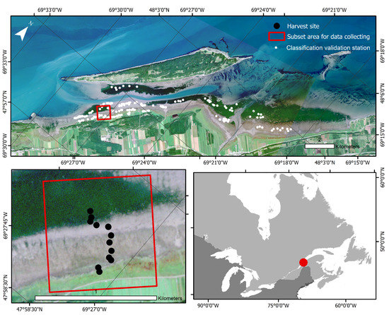
Figure 1.
True-color image of l’Isle-Verte from PlanetScope captured on 3 September 2019. The outer red box delimits the subset used for the study area, and the black dots identify the 13 harvest sites. White dots on the upper panel are the locations selected for the classification validation.
The sampling site is protected from wave action by the Isle-Verte island (municipality of Notre-Dame-des-Sept-Douleurs) (69°27′00″W; 47°58′30″N). This area is home to one of the largest eelgrass meadows of the St. Lawrence Estuary, a rich and productive environment that has been monitored by the Department of Fisheries and Oceans since the 1980s [27,28]. The climate of the study area is cold (mean annual temperature of 3.5 °C), humid, and highly influenced by estuarine and marine conditions. In the winter, temperatures are well below the freezing point and most of the bay is covered by landfast ice and ice formed along and attached to the shore, also known as ice foot [29] with a mean winter temperature of −10.8 °C. In the summer, the temperatures on the shore remain colder than inland due to the marine influence. The tides are semi-diurnal, with an average tidal range of 3.5 m [30]. The spring tides can reach 4.7 m and are only 1.5 m during neap tides. The estuarine waters are brackish (about 20–25 PSU) and relatively turbid in the study area, limiting the detection of submerged vegetation by remote sensing [30,31,32].
2.2. In Situ Measurement
The sampling area was divided into four zones based on the frequency of immersion, which is a function of elevation, the ice in the winter, the water temperature, and salinity (Figure 2). The zones are: (1) the eelgrass bed of Zostera marina (EG); (2) the mud flat with microphytobenthos (SD: sediment) and the macroalgae zone composed of Fucus and Ascophyllum, mainly attached to scattered boulders (MA); (3) the low marsh cordgrass zone dominated by Spartina alterniflora (SC); and (4) the high marsh zone mainly dominated by Atriplex prostrata (CS, creeping saltbush) [30,31,33]. During the winter, ice scouring creates ice-made tidal pools, which increase the spatial heterogeneity within the shore habitats [34,35,36].
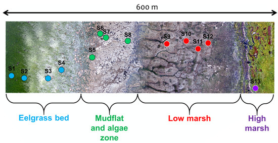
Figure 2.
Drone image collected on 1 September 2019 presenting the delimitation of the four zones of the study site and the transect of 13 harvest points.
A 600 m transect perpendicular to the shoreline was set up to cover the four zones identified above (Figure 2). Thirteen stations, or plots, were placed along the transect, covering each zone of the coast, in relatively homogeneous patches of vegetation (>100 m), except for SD and MA where scattered boulders create high spatial heterogeneity from a remote sensing perspective. A complete species composition list, including the percentage cover estimates, was established for every plot in 50 × 50 cm (2500 cm) quadrats (Table 1).

Table 1.
Zone type, percentage coverage at the beginning and the end of the season, and the vegetation biomass harvested at the end of the season in g/.
Each station was geolocated using a GPS, marked with a wooden post, and visited up to 10 times from 17 May–25 October 2019 (Table 2). All stations were sampled during the low tide, approximately every two weeks during the maximum growth period (defined as mid-May to early August for this study) and then every three to four weeks for the rest of the season until late October due to a decrease of change in the vegetation in the summer, or for practical reasons (instrument availability and other academic activities).
Table 2.
Dates, sky, tidal levels and number of stations of the in situ data collection.
Plant allometry was determined for each station along with radiometric measurements and vertical photographs for the vegetation percent cover (every time). More specifically, plant allometry included the length and width of leaves, and it was determined for eelgrass (EG), the creeping saltbush (CS), and the saltmarsh cordgrass (SC) for every sampling date. For each harvested site, the number of plants (or shoots) were calculated inside the quadrat of ∼2500 cm Furthermore, the number of leaves by plant and their lengths and widths for EG and SC were measured on five plants chosen randomly inside the station. For the CS, the lengths of the stems were measured using five plants, chosen randomly. The lengths of the leaves and stems were measured using tape directly on the field. Solely at the end of the season, the vegetation inside the quadrat was harvested for biomass determination. The leaf area index (LAI) was calculated using a similar method by [37] and applied for the EG and SC. Three shoots were collected in the field and photographed with their leaves (flattened out on a white board next to a ruler). The leaf surface area () was determined using the wand tool of ImageJ software [38]. was measured twice for the photosynthetic leaf surface (using only the green parts of the leaves) and for the total leaf surface (including the necrotic tissue). The LAI was then calculated based on the following, by Watson [37]:
where is the mean surface area (cm) measured for the three shoots of a given quadrat and shoot density () is the density (N shoots m) for the original value for the same quadrat.
2.2.1. In Situ Radiometry
Field radiometry was performed using a VIS-NIR analytical spectral device (ASD) spectroradiometer (Handheld2-pro model) recording wavelengths from 325 to 1075 nm. The upwelling radiance (L, Wmsrnm) spectra were measured at nadir. To avoid any disturbance of the light field, the radiance measurements were collected with a 5 m bare optical fiber fitted to the ASD, having a field-of-view (FOV) of 25°. The fiber was attached at the end of a rod fixed to a tripod pointing the surface at nadir from 113 cm above the surface to obtain a ∼2500 cm surface area (Figure 3), similar to the quadrat area. For each spectrum recorded, the ASD collects five spectra and computes the average and standard deviation of the spectra. Before each surface radiance measurement (), a calibrated white reference (Spectralon plate, ) with a known reflectance value was measured (99.57%) at nadir (). At least two sets of measurements (replicates) were made at each site. More measurements were performed under changing illumination due to the presence of thin clouds or cloudy conditions.
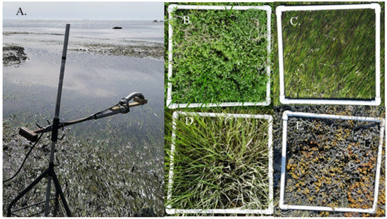
Figure 3.
Acquisition of the emerged surface reflectance with the ASD fitted to a tripod (A) and typical vegetation target photographed at nadir: CS (B), EG (C), SC (D), and MA (E).
The surface reflectance, (unit less), was calculated following Equation (2).
Because the were not collected on the same day and time of the day, under different sky conditions, sun-view geometry, and instrument settings (i.e., integration time) (Table 2), variations in magnitude due to illumination differences were present [39]. Similar issues were noticed in the literature [17], and a correction was then applied to following [40]. Briefly, the multiplicative scatter correction method (MSC; [40,41]) minimizes the uncertainty in the reflectance spectra due to different measurement conditions while keeping the main spectral features. MSC applies a simple correction to the raw reflectance value at each wavelength of the sample spectra based on the reference spectra. It uses the offset and the slope values estimated by linear least-squares regression of all the raw spectra collected in the field against a reference spectrum [41]. In MSC, the linear regressions are fit to a local wavelength region using a moving window of a specified length. The reference spectra applied in the MSC to the sample spectra were the mean spectra of each station’s spectra collected during the growing season.
The spectral similarity between the spectra was estimated using the spectral angle mapper (SAM; rad), used [42] as:
where B is the number of spectral bands, k the ith waveband, x and y are two spectra to compare, respectively. The SAM was applied to both raw and MSC-corrected spectra, but only the latter were used for further analysis. The SAM was used to examine the spectra similarities/differences among different species, and for a given species during the growing season.
2.2.2. Spectral Resampling and Vegetation Indices
For comparison with satellite data, the measured hyperspectral were resampled to the multispectral bands of OLI, MSI, RapidEye, and PlanetScope using the sensor spectral response function (SRF) provided by the space agencies. For all sensors, only the visible and the near-infrared bands (400–900 nm) were used for the analysis.
Many different vegetation indices (VIs) have previously been applied to multispectral remote sensing data [43]. In the present study, VIs suitable for the satellite sensors were tested (Table 3) to identify which indices respond best to seasonal variability and vegetation density metrics (i.e., LAI).
Table 3.
Vegetation indices applied to the reflectance spectra and the satellite images.
2.3. Satellite Data
Cloud-free satellite images from OLI, MSI, RapidEye, and PlanetScope captured between May and October 2019 were downloaded for the data providers (USGS EarthExplorer, earthexplorer.usgs.gov; Copernicus Open Access Hub, scihub.copernicus.eu; and PlanetExplorer planet.com/explorer/ all accessed on 16 June 2022).
A total of 16 images (Sentinel-2 (6), Landsat-8 (2), RapidEye (2), and PlanetScope (6)) were selected based on the date, the state of the tide, and the cloud cover, i.e., a low tide under a clear sky (less than 15% of cloud cover) (Table 4).
Table 4.
List of the images acquired for the study and the water level when the sensor collected the images.
Level 1 images (top-of-atmosphere radiance) were atmospherically corrected to retrieve the surface reflectance using ACOLITE (version Python 20190326.0), which was adapted for all sensors. To compute the surface reflectance, the dark spectrum fitting method was adopted using the standard parameters proposed by ACOLITE [48]. Briefly, after cloud masking and gas transmission correction of top-of-atmosphere reflectance, ACOLITE found multiple dark pixels in sub-scenes, to define a “dark spectrum” based on the lowest reflectance values in any spectral bands. The dark spectrum was then used to estimate the atmospheric path reflectance according to the best fitting aerosol model. Sky and sun glint components were also estimated over water surfaces, but not for land surfaces. The images were then projected, and the VIs were calculated. The homogeneous area of each vegetation species and sediment were delimited based on GPS collected on the field and from drone images (collected in September) to compare VIs from the images to the in situ. The VI values were extracted from those areas covering the stations visited in the field. For MA, due to the small patch size, subpixel fractions were calculated based on the sensor’s pixel size using a very high spatial resolution drone image. For each area, the mean values of the VIs were calculated.
2.4. Classification
Image classification was performed using a machine learning algorithm named the extreme gradient boosted decision tree algorithm (hereafter referred to as XGBoost) [49]. To classify the vegetation, the XGBoost creates decision trees based on the input features and assigns specific weights to these features based on their significance in identifying a vegetation species, thereby defining the feature importance for the model. To train the XGBoost model, the in situ spectra associated with each vegetation type and sediment were used [50]. The in situ dataset was divided into training and testing datasets with a 4:1 ratio to train the model effectively. We first trained the model using the of each vegetation type and sediment collected during the growing season. This model was applied to the Sentinel-2 image time series (hereafter referred to as XGBoostnoSeason). Six images were classified from June to October (one per month). To cover all months of the growing season, an image from August 2020 was used as no clear sky images were available in August 2019. This process allowed us to identify the most favorable month to distinguish intertidal vegetation. Furthermore, to identify the best period in the season to classify the intertidal coastal habitats, XGBoost models were trained using the in situ collected closest to the date of the satellite image acquisition (hereafter referred to as XGBoostSeason).
The classification accuracy was evaluated using 170 different data points for which the vegetation classes were known based on the information collected from the study area and photo-interpretation of the drone or aerial photographs (white dots on Figure 1). A confusion matrix was generated and the overall accuracy, Kappa coefficient (), and per-class F1-score were calculated to assess the performance of the classification. The values ranged between 0 and 1; they are measures of accuracy that account for the random chance of correct classification [51]. The F1-score (ranging between 0–1) is the harmonic average of precision and recall for every class to deal with unbalanced validation data [52].
2.5. Satellite Vegetation Index Validation
The VI values from the reflectance spectra (in situ) and the multispectral satellite images were statistically analyzed for the different vegetation types. It was then possible to determine whether the VI values between vegetation types differed between in situ and satellite data. The accuracies of the satellite VI retrievals were evaluated using the root mean square error (RMSE), the mean relative difference (Bias), and Pearson’s correlation coefficient (r), expressed respectively as:
where N is the number of samples in the data set, the in situ value, and the satellite estimated value of the parameter of interest; and are the corresponding mean values of the samples. We used a significance level of = 0.05 for all statistical analyses.
3. Results
3.1. Field Observations
3.1.1. Biophysical Parameters
Over the season, the number of leaves per shoot, the leaves, and the stem maximum length for Zostera marina (EG), Spartina alterniflora (SC), and Atriplex prostrata (CS) were measured (Figure 4A). For the SC and the CS, the maximum length increased from May to August, with lengths reaching about 35 cm (except for station S9 that remained shorter than 20 cm), which was 30 times longer than at the beginning of the season in mid-May. A sharp decrease in the absolute length of the stem and leaves occurred after the peak reach in August, with leaf length values at ∼10 cm in October. In contrast, the EG leaf length at the beginning of the season was much longer (10 to 25 cm) than the other species. It must be noted that the length of the leaf was inversely proportional to the elevation relative to the sea level, with longer leaves in deeper waters (S1–S3). More than twice shorter leaves were observed at station S4 located at the fringe of the meadow in sightly shallower waters (Figure 2). The maximum lengths of the eelgrass leaves increased until September, reaching lengths >20 cm with a maximum of 80 cm and the absolute lengths decreased at all stations thereafter.
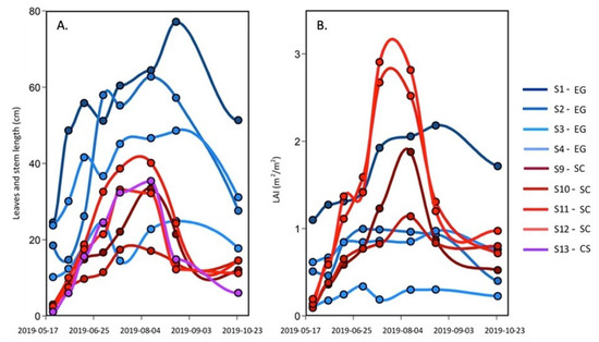
Figure 4.
Seasonal evolution of (A) the leaves and stem maximal length and (B) the leaf area index (LAI) of the EG and SC, and the steam length of the CS from 23 May–25 October 2019.
The leaf area index (LAI), a commonly used proxy to quantify the density of vegetation canopy, allows the estimation of the plant canopy surface area per m of the substrate (Figure 4B). For the EG, the LAI was somewhat more stable throughout the season and lower than the SC in the middle of the summer. The seasonal evolution of EG LAI is explained with tissue growth until August, and thereafter—a decrease (due to the appearance of necrosis on the leaves, which reduced the LAI based on the green part of the leaves). As for the SC, the LAI increased from May to July (S11 ad S12) or August (S9 and S10) reaching values > 1 m m (maximum close to 3 m m), and then decreased to values of 0.5 to 1 m m in October due to the pigment degradation in the tissue caused by the temperature change.
3.1.2. Spectral Signatures of Vegetation Types and Sediments
Figure 5 presents the average and standard deviation (shaded area) of each vegetation type calculated on all available raw and MSC-corrected , respectively. As expected, much larger variability was observed in raw spectra compared to the MSC-corrected, which was due to the seasonal evolution of the spectra, but also, to some extent, due to the illumination conditions that varied from date-to-date (e.g., a clear sky versus cloudy or partly cloudy; (Table 2). Despite a marked seasonality in terms of leaf length and LAI (Figure 4), the standard deviation of raw was much lower for Spartina alterniflora (SC) compared to the other vegetation species. The largest variability was observed in the NIR for creeping saltbush, followed by macroalgae and eelgrass. A homogeneous spectral variability was also observed for bare sediments, except a notable trough around 676 nm corresponding to the red peak of absorption because of chlorophyll-a. The MSC normalization removed most of the variability, including part of the seasonal variability. Interestingly, the spectral shape of the MSC-corrected spectra for MA in the visible bands showed virtually no variability, suggesting a very stable pigment composition across the growing season for this type of vegetation. For comparison, EG and SC showed the largest variability in the visible bands after the application of the MSC, followed by SD.
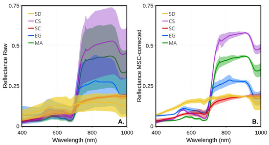
Figure 5.
Mean reflectance spectra of four vegetation species and sediments and their standard deviations (shaded area): (A) raw ; (B) MSC-corrected .
The SAM quantifies the spectral similarity and difference between the vegetation species (Figure 6). Sediment (SD) spectra differed markedly from all vegetation types (SAM > 0.29 rad), with the largest difference with MA. The spectral differences between the EG and MA, EG and CS, and MA and SC showed intermediate values (0.23 < SAM < 0.27 rad). Between the different vegetation types, MA and CS showed the smallest differences (0.1 rad), followed by SC versus CS (0.17 rad).
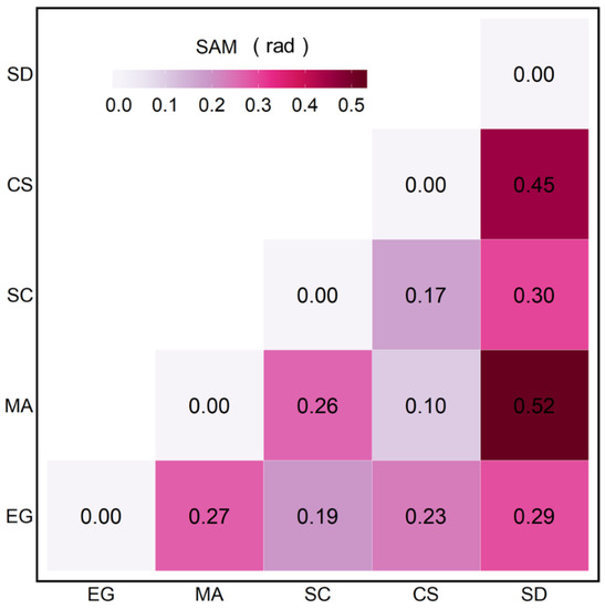
Figure 6.
SAM analyses were applied to the MSC-corrected of four vegetation species and sediments.
3.1.3. Spectral Phenology
In general, the spectral shape of vegetation species remained almost the same throughout the season. However, there can be spectral crossovers between species due to changes in the absorption strengths and pigment concentrations. Therefore, it is necessary to consider intra- and inter-species spectral variability throughout the season.
In the visible spectrum, the reflectance peak of the healthy EG was stable over the season and was located between 555 and 564 nm (Figure 7C). The EG showed a very low reflectance peak at the beginning of the season (early May) before jumping up to the highest reflectance for this season at the end of May. Afterward, the spectra remained, with mid- to low peaks and values observed in the middle and at the end of the season. Two major absorption bands were visible and located in the blue (489–496 nm) and red (671–677 nm), respectively. Those absorption bands are typical of the absorption features of chlorophyll and carotenoids. Note that the spectrum observed on 23 May differed from the other. The exact reason for this anomaly could not be confirmed due to the unavailability of supporting data. At any other moment through the season, the EG spectra stayed similar without a clear seasonal evolution.
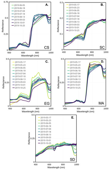
Figure 7.
MSC-corrected reflectance spectra collected through the summer for four vegetation species and sediments collected from 17 May to 25 October 2019 for CS (A), SC (B), EG (C), MA (D), and SD (E).
The macroalgae spectra remained stable over the season (Figure 7D), with almost no change in the visible range compared to the NIR. The location of the green reflectance peak was regular, around 568 to 574 nm. Still, two absorption bands could be located, one in the green (504–520 nm) and the other in the red (671–678 nm). Secondary reflectance peaks are found in the red near 650 and 670 nm, respectively (c.f. Figure 7).
The peaks of reflectance of CS and SC were shifted to the longer wavelengths in the beginning (May to end of June) and at the end (mid-September to November) of the season (Figure 7A,B), but were almost the same as the EG in the middle of the summer (July to the middle of September). For the SC, the peak reflectance location shifted from 556 to 648 nm from the summer to the fall (Figure 7B). As for CS, the reflectance peak was located between 554 nm in the summer and shifted to 648 nm in October (Figure 7A). Both species presented similar absorption bands in blue (488–499 nm) and in red (672–680 nm) portions of the visible. The later corresponds to the red absorption peak of chlorophyll-a. The seasonal shift in the reflectance peak can be explained by the composition of the dominant pigment changing at the beginning and end of the season.
SAM was used to assess the seasonal variation in the spectral reflectance for each vegetation type and bare sediment (Figure 8). For MA and SC, the spectra did not change over the season with SAM values constantly below 0.18 and 0.14 rad, respectively (Figure 8B,D). Even though the SAM values were low for SC, we observed a difference in the spectral shape between the beginning/end and the middle of the season, but the differences remained small in terms of SAM. For example, the August spectrum was clearly different relative to the spectra measured in May, June, and the end of October (0.11 < SAM < 0.14 rad; c.f. Figure 8B). Among the four vegetation types, the CS showed the clearest seasonal evolution in terms of reflectance (Figure 8A). The values obtained by the SAM ranged from 0.02 to 0.27 rad. Spectra at the beginning (May and June) and at the end (September and October) of the season were similar, and different from those from the middle of the season (July to August). As for EG, the SAM values ranged from 0.04 to 0.38 rad (Figure 8C), with an anomalous value for the spectra collected on 23 May. The high SAM values for those spectra may be attributed to a particular moment corresponding to a high EG growth rate, or to the unstable sky conditions while collecting in situ radiometric data. As mentioned previously, the exact reason for this anomaly could not be confirmed due to the unavailability of supporting data. At any moment, the EG spectra stayed remarkably similar without a clear seasonal evolution.
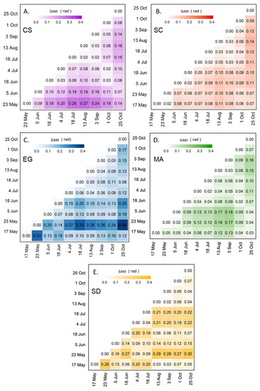
Figure 8.
SAM analyses were applied to the reflectance spectra of four vegetation species and sediments collected from 17 May to 25 October 2019 for CS (A), SC (B), EG (C), MA (D), and SD (E).
Figure 9 shows the SAM calculated for a vegetation type using the spectra at a given date, against another date. This analysis helps to understand the variations of spectral changes of a species relative to another during the summer season. The most significant difference between all vegetation species spectra occurred at the beginning (May and June) and the season’s end (September and October). For example, Figure 9A compares creeping saltbush (CS) with the other vegetation types (EG, MA, SC) and sediments (SD). The largest difference between CS and the other was in May, except for SC, where the SAM remained stable during the growing season (0.2 rad). In June and July, CS and MA were very similar and difficult to distinguish spectrally (SAM < 0.1 rad) Figure 9A,D. A similar remark can be made for EG, where the lowest SAM were generally found in July. It also suggests that EG differs more from the other vegetation types in the spring (end of May) and in early October. Saltmarsh cordgrass (SC) is more easily distinguished from EG and MA at the beginning and end of the season (Figure 9B), but more different from sediment in July. The sediment spectra are different from all ofthe vegetation spectra (Figure 9E). Overall, this analysis indicates that it can be difficult to distinguish many vegetation species based on a single date in the middle of the growing season (June to August).
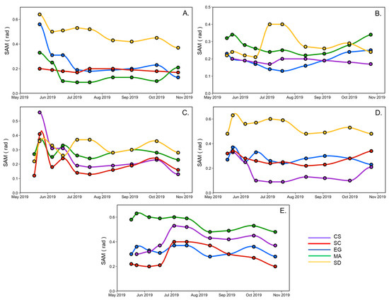
Figure 9.
SAM analyses applied to the reflectance spectra according to the vegetation species and sediment over time, collected from May to the end of October for CS (A), SC (B), EG (C), MA (D), and SD (E).
3.2. Classification of Vegetation Type
To examine the implication of spectral and seasonal variability of the vegetation type for mapping the coastal intertidal zone using multispectral imagery, a classification algorithm was applied to the Sentinel-2 MSI time-series covering the growing season (Table 4). This sensor was selected because (i) it provides the best response to seasonal variability and availability over the critical dates for the vegetation phenology; and (ii) it has 13 spectral bands, including key bands in the red-edge portion of the spectrum that is suitable for vegetation mapping.
The XGBoost algorithm was first applied to the image using the in situ spectra associated with the date closest to the acquired image (XGBoostSeason, Figure 10). By changing the input spectra, the algorithm demonstrated a successful identification of the vegetation species, which confirmed the occurrences and spatial distributions by each species (Table 5). For the first and last images (May and October), most of the classification mistakes were due to confusion between saltmarsh cordgrass (Spartina alterniflora, SC) and the sediment (not shown) due to their similar spectral signatures at this time of the year (Figure 9B,E). On every image, the algorithm seems to have a problem identifying the macroalgae (MA). This might have been caused by the spatial resolutions of the images and the sizes of the MA patches attached to the boulders that were generally smaller than the pixel sizes. Note that none of the classified images present MA on the rocky shores of the island (west tip and north east coast of the island). Based on the classification evaluation metrics (overall accuracy and indices; (Table 5), early June and the end of September images were best suited for the coastal vegetation cover mapping. In other dates, the overall accuracy reached about 70% with the worst performance obtained in October (accuracy of 65% and of 0.56).
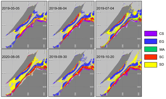
Figure 10.
Classification of coastal and intertidal vegetation using XGBoostSeason applied to the Sentinel-2 time series.
Table 5.
Model validation statistics (overall accuracy (), and mean F1-score) of XGBoostSeason.
Even though XGBoostSeason can classify the intertidal zone with significantly good accuracy, it is not practical to train separate models for every month of the growing season. Therefore, we trained a single XGBoost model (XGBoostnoSeason) (Table 6) using the same set of in situ spectra, without accounting for the seasonality. The goal was to evaluate the sensitivity of the classification to seasonal variability in the vegetation spectra. XGBoostnoSeason yielded marked differences in vegetation mapping (Figure 11) throughout the season when spectral evolution was not taken into account. More sediment was identified in May, reflecting the early stage in the vegetation development and/or the low LAI. Macroalgae occupied a relatively large surface area, which was not consistent with the field observations. As expected, the classified image from May has the lowest accuracy and index (57% and 0.44, respectively). Between May and June, we see an expansion of the EG and SC surface areas. The images from July and August have a problem identifying other vegetation types than EG. In the summertime, the vegetation spectra from all types were too similar and could not be distinguished by the model trained without accounting for the seasonality in . The best performance of XGBoostnoSeason was obtained in September, with accuracy and values of 87% and 0.85, respectively. At this time, the vegetation was fully grown and the senescence had just started, yielding spectrally distinguishable surfaces. The October image yielded the second-best classification metric despite some senescence within the vegetation. It is interesting to note that the October image did not perform as well with the in situ spectra associated with the same date. Although the results of the two classifications for the October image are quite different, the validation results are almost similar. This can be explained by confusion from the algorithms between different species. For example, in the XGBoostSeason, the majority of the confusion is with the SD and the MA, while in the XGBoostnoSeason, the confusion is between SC and SD, resulting in similar validation statistics.
Table 6.
Model validation statistics (overall accuracy (), and mean F1-score) of XGBoostnoSeason.
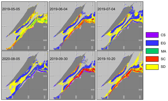
Figure 11.
Classification of coastal and intertidal vegetation using XGBoostnoSeason applied to the Sentinel-2 time series.
Overall, only the eelgrass meadows were well classified (>85% accuracy) in all images, although they were over-represented in the middle of the summer. In contrast, confusion between MA and EG was observed for most images, as observed on the rocky coast of the island at the western tip and along the northeast coast.
3.3. Remote Sensing of Coastal Vegetation Phenology
We further assessed the potential of recent satellite constellations to monitor the phenology of intertidal vegetation found in the study area. The VI time series were computed on both in situ and satellite-derived from OLI, MSI, RapidEye, and PlanetScope. We first evaluated the robustness of each VI in terms of its capacity to predict the leaf area index (Section 3.3.1), a classical proxy for vegetation biomass, as well as its response to the seasonal variability in the vegetation. It turns out that the NDVI provided the highest correlation with LAI, which was selected for further analysis. After a comparison of in situ NDVI (NDVI) with satellite-derived NDVI (NDVI) (Section 3.3.2), we examined the potential of this spectral index to monitor coastal vegetation phenology in our study area (Section 3.3.3).
3.3.1. Vegetation Indices as Predictor of LAI
Among the VIs listed in Table 3, the NDVI presented the best predictor of the LAI (highest r and RMSE). Figure 12 shows the linear relationship between LAI and the NDVI for EG and SC, separately. For both species, we found an important variability in terms of LAI at some stations at a given NDVI value. This is particularly evident at stations S1 and S2, where a dense EG cover (100% coverage throughout the growing season) produced almost constant NDVI value, while the LAI varied by a factor of 2. At other stations where the initial % coverage was lower (Table 1), seasonal variability was more evident, especially for the SC. Note that the MSC correction of tends to reduce the variability in NDVI, but increases the Pearson correlation with the LAI (Table 7), confirming the relevance for that correction.
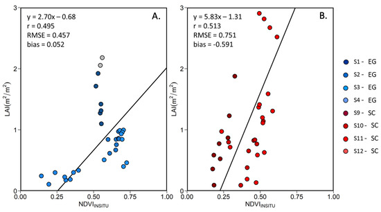
Figure 12.
Linear relationship between the in situ MSC-corrected NDVI and LAI for (A) EG and (B) SC. Grey data points represent outliers.
Table 7.
Pearson’s correlation coefficient (r) of the LAI versus VI relationships obtained for EG and SC. The highest (bold) and lowest (italic) values are highlighted.
3.3.2. Satellite-Derived NDVI Validation
Within a given time frame of two days, 15 match-ups, i.e., co-incident in situ and satellite observations, were obtained considering the four satellite sensors evaluated (Figure 13). The relatively strong linear relationship (r = 0.76) between the MSC-corrected NDVIin situ and NDVI, and the low bias (−0.054) and RMSD (0.16) indicate good agreement between the in situ and satellite NDVI. The NDVIin situ values followed were clustered by vegetation type showing that the MA had the lowest values, followed by SC, EG, and CS. For all sensors, a much larger range of NDVI (−0.24 to 0.95) was obtained compared to NDVIin situ (0.13 to 0.75). This was also true for individual vegetation types (e.g., MA and EG), where the NDVIin situ varied in a narrow range compared to the satellite retrievals. One explanation for the low range in NDVIin situ was due to the MSC normalization of the in situ spectra (see below). Sentinel-2 MSI and Landsat-8 OLI presented the best relations between the NDVIin situ and satellite values. The RapidEye and PlanetScope sensor provided generally good results for most of the vegetation species, except for the MA. These sensors had lower spectral resolutions (i.e., broad spectral bands), yielding outliers, as shown in Figure 13.
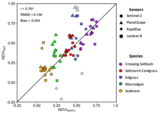
Figure 13.
Scatter plot of in situ and satellite-derived NDVI. Different symbols are for sensors and colors for vegetation types (see legend). Grey data points represent outliers.
3.3.3. NDVI-Based Phenology
Figure 14 shows the seasonal evolution of NDVI for each vegetation type calculated from the in situ MSC-corrected (solid lines) and raw (dashed lines) reflectance spectra. Interestingly, there is not much crossover with the NDVI value among species; each has its specific range (as in Figure 13). The shape and range is similar for both normalized and raw spectra for SD and MA, but the normalization reduces the range for CS, SC, and EG. As expected, bare sediment (SD) or mud had the lowest NDVI values (<0.15), followed by SC, EG, CS, and finally MA. For SD and MA, the NDVI was relatively constant over the season with values of 0.04 ± 0.11 and 0.82 ± 0.07, respectively. Note that MA NDVI was for “pure” spectra while satellite-derived MA NDVI values considered the subpixel coverage (sediment mixed with MA). We can see a clear seasonal evolution for the CS with NDVI as obtained from MSC-corrected reflectance ranging between 0.44 and 0.76. For SC, the NDVI peaked in August at 0.49 and was minimum in May with a value of 0.33. For these two vegetation types, in particular, the MSC-correction substantially reduced the range of variability Figure 14. EG NDVI constantly increased from May to early October when computed on MSC-corrected spectra but showed two peaks in early July and early September when computed on raw spectra. Note that the decrease in NDVI in mid-summer (July–August) was likely due to the presence of necroses in the leaves. EG seasonal evolution also varied among stations with more marked evolution at S3 and S4 where the initial coverages were 50% and 20%, respectively (Table 1; Figure 4).
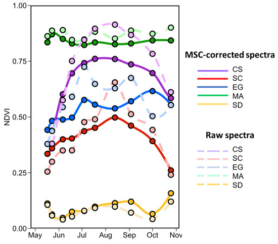
Figure 14.
Temporal evolution of the NDVI values from the in situ spectra collected from May to the end of October of four vegetation species and sediments. Dashed lines are NDVI calculated on raw reflectance spectra.
Since only two images were available for Landsat-8 OLI and RapidEye sensors, respectively, we assessed the space-based phenology using Sentinel-2 and PlanetScope constellations. Six images were available for the Sentinel-2A and 2B MSI sensor from May until the end of October 2019, covering most of the critical moments for the coastal and saltmarsh growing season (Figure 15), but with a more than 2-month gap between 4 July and 12 September.
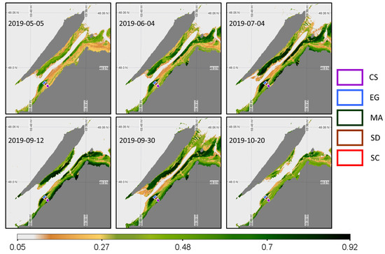
Figure 15.
Time series of NDVI from the Sentinel-2 MSI acquisition obtained at a low tide. Homogeneous regions of interest (ROIs) for the four vegetation types and sediments where the NDVI values were extracted are also shown.
Eight images from mid-May to early October 2019 were available for the PlanetScope sensor (Figure 16). PS images filled the gap of MSI images, but no images beyond October 3 were available for the senescence period.
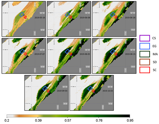
Figure 16.
Time series of NDVI from the PlanetScope sensor acquisition obtained at a low tide and zoomed in on the region of interest. Homogeneous regions of interest (ROIs) for the four vegetation types and sediments where the NDVI values were extracted are also shown.
Figure 17 depicts the phenology of NDVI by combining the two satellite sensors for the pixels extracted from five homogeneous regions of interest (ROI) located in the sampling area (Figure 16). Steady growth in NDVI for all vegetation types was identifiable from May to August, while the sediment stayed relatively constant. The agreement between MSI and PS was very good for CS and SC throughout the season, except in September/October for SC. The phenology of these two vegetation types agree well with in situ observations (Figure 14) with peaks in August reaching 0.75 and 0.55 for CS and SC, respectively.
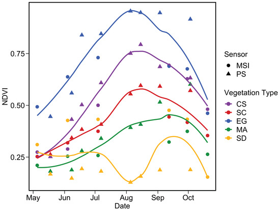
Figure 17.
Satellite-based phenology of coastal vegetation from MSI and PS sensors for the four vegetation types and sediments. NDVI pixels values were extracted from homogeneous surfaces depicted in Figure 16. The LOESS fit was applied for each vegetation type to better visualize the phenology.
A more noisy signal was obtained for EG, which showed higher NDVI relative to other vegetation types. This result contrasts with in situ observations (Figure 14), but not with Figure 15 and Figure 16 where dense EG stations (S1 and S2) constantly showed higher NDVI compared to NDVIin situ. EG mapping was more sensitive to tidal differences among satellite acquisitions as it stood in deeper water (e.g., <0.2 m above sea level) relative to CS and SC. The phenology of this vegetation type was more evident from space than for field observations probably due to the percentage coverage of our selected stations.
Macroalgae phenology extracted from satellite images was more pronounced than expected from the in situ observations. Again, the large difference in MA phenology between in situ and the satellite was due to the spectral resolution versus the size of the vegetation patches. The lack of a continuous cover of MA limited our interpretation for this type of vegetation. The SD showed the lowest values and remained relatively constant throughout the season for a given sensor, although a small peak was observed in the late summer. A relatively important discrepancy was obtained between MSI and PS. The later yielded NDVI within the range of the in situ data with non-seasonal variability. In contrast, MSI values for the sediments were relatively high (0.25 to 0.4).
In summary, the images from PS and MSI sensors, allowed us to detect the seasonal evolution of the vegetation. By combining the time series of the two sensors, we can better see the complementary data, offering a better understanding and monitoring of the phenology of the vegetation.
4. Discussion
In this study, we showed that spectral seasonal evolution in coastal and intertidal vegetation types can be detected by in situ and spaceborne sensors. This evolution is related to the biophysical metric of the vegetation, such as the LAI, but it depends on the vegetation type and the pigment composition. A better understanding of the vegetation phenology provides key insights for the coastal mapping based on spectral classification, with strengths and limitations discussed in the following sections.
We observed an important evolution of the vegetation biophysical metrics, with a growth phase from May to September, which was particularly evident for saltmarsh cordgrass (Spartina alterniflora) and creeping saltbush. This observation was consistent with other studies [53,54,55]. For eelgrass, the growth continued until the beginning of October, while the LAI showed an increase between May and June, remained constant until September, and was followed by a small decrease at the end of the season. Similar results were shown in other studies [56,57,58].
Our vegetation spectra measurement is consistent with other studies [17,59,60,61]. The in situ spectra analyses suggest that the general shapes of are similar for all vegetation types (EG, MA, SC, and CS), but markedly different from the SD. Even if the shape is similar, they are different from each other and evolve over the season, as demonstrated using the SAM and the NDVI. This seasonal evolution is crucial for ecosystem remote sensing and is rarely mentioned and documented in other studies [62]. The spectra from mid-June to the beginning of September often overlapped. At that time of the growing season, the distinction among vegetation types was less obvious. Furthermore, the evaluation of the pure vegetation spectra revealed that MA and EG were stable throughout the season under 100% cover. In contrast, CS and SC presented more variability during the growing season with similar spectra at the start (May and June) and at the end (September and October), but different in the middle of the season (July to August).
Sentinel-2 images were chosen to classify the intertidal and coastal vegetation types in the study area. Using the identical spectra for all images, the XGBoost algorithm (XGBoostnoSeason) was not able to distinguish the vegetation types in July and August. Nevertheless, good results were obtained in June and at the end of the growing season (September and October). The highest accuracy ( of 0.85) was obtained with the September 30th image at the onset of the senescence phase, suggesting that fully-grown vegetation is spectrally distinguishable from each other. We also demonstrate that accounting for vegetation phenology in the classification training dataset (XGBoostSeason) improved the classification accuracy by about 15%.
The NDVI was the most suitable proxy for the LAI among different VIs, and it was selected to evaluate the phenology from remote sensing using in situ spectra and multispectral images from four sensors (Landsat-8 OLI, Sentinel-2 MSI, PlanetScope, and RapidEye). The NDVI has been widely demonstrated to be a good descriptor of vegetation dynamics for many types of ecosystems, including wetlands [17,63,64,65,66]. It is also widely used in satellite-based phenology monitoring, as it could be applied to almost any multispectral sensors on a wide range of platforms (in situ, drone, plane, satellite) [67,68]. Based on in situ NDVI measurements, SC and CS clearly showed a seasonal evolution, while MA, EG, and SD were more stable throughout the season. Frequent observations are needed to quantify the seasonal variability and evolution of the vegetation in a cold temperate environment due to a relatively short growing season (<6 months). Changes in coastal vegetation, such as growth, flowering, senescence, and shedding of leaves, take weeks and even months [68,69,70]. For this reason, we recommend visiting the field as soon as the ice starts to melt (i.e., late March or beginning of April) [69,71]. In our study, we started the fieldwork in mid-May when the EG was already growing, with some stations showing 100% areal coverage.
By combining MSI and PS images, we could also track the vegetation phenology with a clearer signal for EG compared to the in situ. In general, satellite-derived phenology was consistent with the in situ NDVI values shown in this study and as presented by [17,60,72,73]. For example, Zoffoli et al. [17] also used MSI images to document the phenology of intertidal seagrass (Zostera noltii) in France. For comparison, these authors obtained 22 MSI images obtained at a low tide under cloud-free conditions for a ten-month period (March to December). With only six MSI images in our region, the combination with the PlanetScope constellation was necessary to fully capture the growing seasons and the following senescence. However, if our result demonstrates the feasibility, differences in spectral and spatial resolutions between sensors may complicate the combination of multisensor data for phenology monitoring.
As for Landsat-8 and Sentinel-2—both EO missions are dedicated to land cover monitoring and are widely used for phenology assessment. They both acquire images at lower temporal and spatial resolutions compared to PlanetScope. Even if the images are not available at a rapid rate due to tidal height and cloud cover restrictions, we can expect monthly images for the Sentinel-2 sensor, but much less for Landsat (one or two per year). Sentinel-2 images are easily usable and provide much better spectral resolution compared to the very-frequency acquisition of PlanetScope. Therefore, Sentinel-2 images allow further mapping capability by applying a classification algorithm using a high number of bands ( 10 bands). Still, Landsat is a very useful sensor, offering long-term time series for detecting and relatively good spectral capability for coastal mapping [74,75,76]. In addition, the temporal resolution will improve with the recent launch of Landsat-9 in September 2021, opening the door for data fusion from MSI and OLI [73,77,78]. The fusion of Landsat and Sentinel-2 images has tremendous potential to improve the ability to detect vegetation change and to cover all key periods of the vegetation phenology. However, in our case, combining the data was not necessary because the Sentinel-2 time series was already covering all of the vegetation phenology.
The PlanetScope sensor constellation is relatively new and offers many advantages, including high temporal resolution obtained at high spatial resolution compared to Landsat and Sentinel-2. Those images appear to be promising for extracting natural resources information, including intertidal ecosystem estimates and potentially even vegetation diversity estimates [20,79,80]. As seen in our results, the sensor provides many images covering most of the vegetation key. The spatial resolution of PlanetScope images provides many details, but it is not without issues. Indeed, the variable radiometric quality, inconsistent radiometric calibration across multiple platforms, and low spectral resolution are central challenges for marine and coastal applications, such as vegetation classification and ecosystem monitoring [20,81,82,83]. The low spectral resolution of the first Dove generation limits its use for the vegetation type classification. Furthermore, the noise level is high, and the radiometric quality and inconsistency are low on clusters of pixels, especially in homogeneous pixels. This indicates the low signal-to-noise ratio of PlanetScope images [20,84]. This issue was encountered during the atmospheric correction, and even after the correction, noise can still be detected in the NDVI images. The next generation of PlanetScope sensors launched in January 2022 with a greater number of bands (eight bands) and a radiometric signal that may have helped resolve most of the limitations of the early sensor fleets.
The presence of water overlying the vegetation at the time of in situ data acquisition or in the images highly affected the spectral reflectance due to its high absorption in the red and the infrared. With high water levels within the vegetation, the species identification can be difficult, and further processes will be needed to use the images and spectra [85,86,87,88]. For this reason, the state of the tidal level could significantly influence the spatiotemporal distribution of remotely-sensed parameters, such as vegetation NDVI, which uses red and infrared wavelengths. For example, the bathymetric map combined with water level measurements during the data acquisition could be used to correct the water column interference to retrieve the bottom reflectance [88]. However, estuarine water masses of the St. Lawrence are characterized by high concentrations of colored dissolved organic matter (CDOM) and suspended sediments that severely limit the light penetration, even in the visible bands [89], and impair water column correction. Due to the loss of spectral information in the NIR, submerged vegetation indices need to be based on visible bands only [40,88], or located in the red-edge portion of the spectra [59]. In conclusion, we recommend selecting images at the lowest tides possible to maximize the area to be mapped and to minimize the effect of water on the vegetation. The maximum tidal height that allows the vegetation to be mapped using multispectral data requires prior knowledge of the area. Furthermore, the mapped area will mainly depend on the area characteristics, such as the bathymetry/elevation and location of the vegetation.
Many atmospheric correction (AC) algorithms can be applied to multispectral images; this is a crucial step in the processing of remote sensing data for aquatic and coastal applications. Ideally, AC aims to separate the top-of-atmosphere observation by the satellite sensor into the signal from the atmosphere and the signal from the surface to retrieve surface reflectance [90]. By using PlanetScope and RapidEye sensors, we are limited by the atmospheric correction algorithm due to a lack of spectral bands (as, for example, in the SWIR). Even though we can apply different atmospheric corrections, the algorithm applied to the image needs to be the same to compare the sensors together. Here, we adopted ACOLITE, as it allows the application of the dark spectrum fitting (DSF) atmospheric correction method to all imagery evaluated in this study. Furthermore, ACOLITE has been developed for the coastal environment and is currently widely used for aquatic-based applications, such as coastal water monitoring [91,92,93,94]. The sensitivity of satellite-derived NDVI phenology to AC could have been quantified, which was out of the scope of this study.
The area covered by our sampling sites was minimal (472,800 m) as we focused our effort on one EG meadow and intertidal vegetation section to maximize our frequent visits to the sites. This area was selected for its diversity of vegetation cover and easy access but was nevertheless quite representative of the entire coast of the region. The small size of the studied area helped us to develop excellent knowledge of the vegetation dynamics and the ecosystem structure. However, the sites were not optimal for the detection of small macroalgae patches (e.g., <1–2 m) with the limited satellite spatial resolution.
5. Conclusions
In this work, we assessed the seasonal dynamics of four typical intertidal vegetation types encountered in cold temperate coastal littoral, including macroalgae (Ascophyllum nodosum and Fucus vesiculosus), eelgrass (Z. marina), saltmarsh cordgrass (S. alterniflora), and creeping saltbush (A. prostrata). The seasonal evolution was determined based on biophysical characteristics (leaf area index), in situ reflectance spectra, vegetation indices, and classification of multispectral images. We identified a significant seasonal change in phenology of saltmarsh cordgrass and creeping saltbush. Even though some seasonal change could be observed for some vegetation types, no significant changes were observed in the in situ reflectance spectra for eelgrass and macroalgae. Moreover, we evaluated the potential of the NDVI to quantify the vegetation phenology from space. We demonstrated that the NDVI was the best vegetation index proxy to track the phenology that could be applied to multispectral cameras (including drones). Satellite-based NDVI, which strongly correlates with in situ values for saltmarsh cordgrass and creeping saltbush, were used to assess the potential of multispectral instruments to assess the phenology. By combining Sentinel-2 and planet imagery, we showed that the seasonal evolution of eelgrass NDVI was more evident than with in situ measures, likely because of the initial coverage of the quadrats (2500 cm). The extreme gradient boosted decision tree (XGBoost) algorithm was applied to a monthly time series of Sentinel-2 using in situ spectra as input spectral classes. The results indicate September as the best month of the year to classify coastal vegetation in our cold temperate environment, i.e., when the vegetation is fully grown and spectrally distinguishable.
Further work is required to monitor the vegetation species from this complex ecosystem located in a cold temperate climate with a relatively short growing season. We intend to extend the vegetation species mapping, especially for marshes that have a high plant diversity (Salicornia maritima, Spartina pectinata, Spartina patens, etc.). Satellite remote sensing provides access to spatial scales, enabling the environment to be documented over vast areas. Widening the study area to cover all the coasts of the St. Lawrence maritime estuary and Gulf system would be interesting to know their conditions and interannual evolution. In addition, it will extend our knowledge of vegetated coastal ecosystems and their overall importance to the environment. Furthermore, it would be interesting to evaluate the carbon stock sequestration rates in coastal habitats (seagrass and marshes). Remote sensing tools are nowadays developed to quantify the extent of seagrasses and marshes, the species composition of these environments, and the above-ground biomass. In addition, some authors have demonstrated the possibility of estimating carbon stocks using empirical algorithms [95,96,97]. With these types of data, it will be possible to document and monitor changes in carbon stocks and estimate emissions as functions of ecosystem degradation, conservation, and restoration. Finally, historical data could be used to assess the history of carbon stocks and emissions and the spatial distribution and changes of vegetation species.
Author Contributions
B.L. contributed to the data collection and processing and wrote the original draft of this manuscript. S.B. supervised the work, came up with the original idea, contributed to the revision, wrote the manuscript versions, and provided funding. R.K.S. contributed to the atmospheric correction of satellite imagery, data processing (XGBoost classification), and revised the manuscript. P.B. co-supervised B.L., contributed to the fieldwork planning, and revised the manuscript. M.C. led the R.Q.M. project (see below) and provided funding. He contributed to the fieldwork planning and revised the latter version of the manuscript. All authors have read and agreed to the published version of the manuscript.
Funding
This research was mainly funded by the program Odyssée Saint-Laurent from the Réseau Québec Maritime (grant number 2018-38-04) attributed to MC (PI), PB, and SB (co-PIs). SB was provided funding from an NSERC discovery grant (RGPIN-2019-06070) and from the WISE-Man Project funded by the Canadian Space Agency through the FAST program (FARIMA18).
Data Availability Statement
The data that support the findings of this study are available from the author upon reasonable request.
Acknowledgments
The authors acknowledge Véronique Thériault and Colin Surprenant for sharing the drone images. The students who contributed to the field work are also acknowledged: Loïc Théberge-Dallaire, Jimmy Mayrand, François Pierre Danhiez, Soham Mukherjee, Romy Léger-Daigle, and Christel Blot. Furthermore, the authors are thankful to the three reviewers for their comments and suggestions, which improved the quality and readability of the article.
Conflicts of Interest
The authors declare no conflict of interest.
Abbreviations
The following abbreviations are used in this manuscript:
| CS | creeping saltbush |
| EG | eelgrass |
| GRVI | green-red vegetation index |
| MA | macroalgae |
| MSI | multispectral instrument |
| NDAVI | normalize difference aquatic vegetation index |
| NDVI | normalize difference vegetation index |
| OLI | operational land imagery |
| PS | PlanetScope |
| RE | RapidEye |
| surface reflectance | |
| SAVI | soil-adjusted vegetation index |
| SC | saltmarsh cordgrass |
| SD | sediment |
| WAVI | water adjusted vegetation index |
| XGBoost | extreme gradient boosted decision tree algorithm |
References
- Boesch, D.F.; Josselyn, M.N.; Mehta, A.J.; Morris, J.T.; Nuttle, K.; Simenstad, C.a.; Swift, D.J.P.; Nuttle, W.K. Scientific Assessment of Coastal Wetland Loss, Restoration and Management in Louisiana. J. Coast. Res. 1994, 1–103. [Google Scholar]
- Zhang, X.; Wang, L.; Jiang, X.; Zhu, C. Modeling with Digital Ocean and Digital Coast; Springer: Berlin/Heidelberg, Germany, 2017. [Google Scholar]
- Cahoon, D.R.; Hensel, P.F.; Spencer, T.; Reed, D.; McKee, K.L.; Saintilan, N. Coastal Wetland Vulnerability to Relative Sea-Level Rise: Wetland Elevation Trends and Process Controls; Springer: Berlin/Heidelberg, Germany, 2006; pp. 53–65. [Google Scholar]
- Gedan, K.B.; Kirwan, M.L.; Wolanski, E.; Barbier, E.B.; Silliman, B.R. The present and future role of coastal wetland vegetation in protecting shorelines: Answering recent challenges to the paradigm. Clim. Chang. 2011, 106, 7–29. [Google Scholar] [CrossRef]
- Nicholls, R.J. Coastal flooding and wetland loss in the 21st century: Changes under the SRES climate and socio-economic scenarios. Glob. Environ. Chang. 2004, 14, 69–86. [Google Scholar] [CrossRef]
- Airoldi, L.; Beck, M.W. Loss, Status and Trends for Coastal Marine Habitats of Europe. Oceanogr. Mar. Biol. 2007, 25, 345–405. [Google Scholar]
- GIEC. Climate Change 2007: Impacts, Adaptation and Vulnerability; GIEC: Genebra, Switzerland, 2009; pp. 214–219. [Google Scholar]
- Harley, C.D.; Hughes, A.R.; Hultgren, K.M.; Miner, B.G.; Sorte, C.J.; Thornber, C.S.; Rodriguez, L.F.; Tomanek, L.; Williams, S.L. The impacts of climate change in coastal marine systems. Ecol. Lett. 2006, 9, 228–241. [Google Scholar] [CrossRef]
- Dekker, A.; Brando, V.; Anstee, J.; Suzanne, F.; Malthus, T.; Karpouzli, E. Remote Sensing of Seagrass Ecosystems: Use of Spaceborne and Airborne Sensors. In Seagrasses: Biology, Ecology and Conservation; Larkum, A.W.D., Orth, R., Duarte, C.M., Eds.; Springer: Dordrecht, The Netherlands, 2006; Chapter 15; pp. 347–359. [Google Scholar]
- Hossain, M.S.; Bujang, J.S.; Zakaria, M.H.; Hashim, M. The application of remote sensing to seagrass ecosystems: An overview and future research prospects. Int. J. Remote Sens. 2015, 36, 61–114. [Google Scholar] [CrossRef]
- Xie, Y.; Sha, Z.; Yu, M. Remote sensing imagery in vegetation mapping: A review. J. Plant Ecol. 2008, 1, 9–23. [Google Scholar] [CrossRef]
- Carlotto, M.J. Effect of errors in ground truth on classification accuracy. Int. J. Remote Sens. 2009, 30, 4831–4849. [Google Scholar] [CrossRef]
- Satyanarayana, B.; Mohamad, K.A.; Idris, I.F.; Husain, M.L.; Dahdouh-Guebas, F. Assessment of mangrove vegetation based on remote sensing and ground-truth measurements at Tumpat, Kelantan Delta, East Coast of Peninsular Malaysia. Int. J. Remote Sens. 2011, 32, 1635–1650. [Google Scholar] [CrossRef]
- Hedley, J.D.; Russell, B.J.; Randolph, K.; Pérez-Castro, M.; Vásquez-Elizondo, R.M.; Enríquez, S.; Dierssen, H.M. Remote sensing of seagrass leaf area index and species: The capability of a model inversion method assessed by sensitivity analysis and hyperspectral data of Florida Bay. Front. Mar. Sci. 2017, 4, 1–20. [Google Scholar] [CrossRef]
- Knyazikhin, Y.; Martonchik, J.V.; Diner, D.J.; Myneni, R.B.; Verstraete, M.; Pinty, B.; Gobron, N. Estimation of vegetation canopy leaf area index and fraction of absorbed photosynthetically active radiation from atmosphere-corrected MISR data. J. Geophys. Res. 1998, 103, 32239–32256. [Google Scholar] [CrossRef]
- Phinn, S.; Roelfsema, C.; Dekker, A.; Brando, V.; Anstee, J. Mapping seagrass species, cover and biomass in shallow waters: An assessment of satellite multi-spectral and airborne hyper-spectral imaging systems in Moreton Bay (Australia). Remote Sens. Environ. 2008, 112, 3413–3425. [Google Scholar] [CrossRef]
- Zoffoli, M.L.; Gernez, P.; Rosa, P.; Le Bris, A.; Brando, V.E.; Barillé, A.L.; Harin, N.; Peters, S.; Poser, K.; Spaias, L.; et al. Sentinel-2 remote sensing of Zostera noltei-dominated intertidal seagrass meadows. Remote Sens. Environ. 2020, 251, 112020. [Google Scholar] [CrossRef]
- Wang, D.; Ma, R.; Xue, K.; Loiselle, S.A. The assessment of landsat-8 OLI atmospheric correction algorithms for inland waters. Remote Sens. 2019, 11, 169. [Google Scholar] [CrossRef]
- Traganos, D.; Reinartz, P. Interannual change detection of mediterranean seagrasses using RapidEye image time series. Front. Plant Sci. 2018, 9, 1–15. [Google Scholar] [CrossRef]
- Wicaksono, P.; Lazuardi, W. Assessment of PlanetScope images for benthic habitat and seagrass species mapping in a complex optically shallow water environment. Int. J. Remote Sens. 2018, 39, 5739–5765. [Google Scholar] [CrossRef]
- Xue, J.; Su, B. Significant remote sensing vegetation indices: A review of developments and applications. J. Sens. 2017, 2017. [Google Scholar] [CrossRef]
- Dekker, A.G.; Brando, V.E.; Anstee, J.M. Retrospective seagrass change detection in a shallow coastal tidal Australian lake. Remote Sens. Environ. 2005, 97, 415–433. [Google Scholar] [CrossRef]
- Proença, B.; Frappart, F.; Lubac, B.; Marieu, V.; Ygorra, B.; Bombrun, L.; Michalet, R.; Sottolichio, A. Potential of High-Resolution Pléiades Imagery to Monitor Salt Marsh Evolution After Spartina Invasion. Remote Sens. 2019, 11, 968. [Google Scholar] [CrossRef]
- Bolton, D.K.; Gray, J.M.; Melaas, E.K.; Moon, M.; Eklundh, L.; Friedl, M.A. Continental-scale land surface phenology from harmonized Landsat 8 and Sentinel-2 imagery. Remote Sens. Environ. 2020, 240, 111685. [Google Scholar] [CrossRef]
- Drake, L.a.; Dobbs, F.C.; Zimmerman, R.C. Effects of epiphyte load on optical properties and photosynthetic potential of the seagrasses Thalassia testudinum Banks ex König and Zostera marina L. Limnol. Oceanogr. 2003, 48, 456–463. [Google Scholar] [CrossRef]
- Marzialetti, F.; Giulio, S.; Malavasi, M.; Sperandii, M.G.; Acosta, A.T.R.; Carranza, M.L. Capturing coastal dune natural vegetation types using a phenology-based mapping approach: The potential of Sentinel-2. Remote Sens. 2019, 11, 1506. [Google Scholar] [CrossRef]
- Babin-Roussel, V.; Didier, D.; Houde-Poirier, M.; Jean-Gagnon, F.; Lacombe, D.; Provencher- Nolet, L.; Morissette, A. L’Île Verte: Portrait du territoire; Technical Report; Département de biologie, chimie et géograpgie, Université du Québec à Rimouski: Rimouski, QC, Canada, 2011. [Google Scholar]
- Martel, M.c.; Provencher, L.; Grant, C.; Ellefsen, H.F.; Pereira, S. Distribution and Description of Eelgrass Beds in Québec; Technical Report; Maurice Lamontagne Institute, Fisheries and Oceans Canada: Mont-Joli, QC, Canada, 2009. [Google Scholar]
- US. Navy. A Functional Glossary of Ice Terminology; US Navy Hydrographic Office: Washington, DC, USA, 1952.
- Environment and Climate Change Canada. Baie-de-L’Isle-Verte National Wildlife Area Management Plan 2018; Environment and Climate Change Canada, Canadian Wildlife Service, Quebec Region: Gatineau, QC, Canada, 2018; pp. 1–76.
- Gauthier, J.; Rosa, J.; Lehoux, D. Les Marécages Intertidaux Dans L’Estuaire du Saint-Laurent; Environnement Canada, Service Canadien de la Faune: Gatineau, QC, Canada, 1980. [Google Scholar]
- La Société De Conservation De La Baie de l’Isle-Verte. Mise en valeur de l’habitat de poisson de la Réserve Nationale de Faune de L’Isle-Verte; Rapport conjoint Société de conservation de la baie de l’lsle-Verte et Groupe Environnement Shooner pour la Direction de la gestion de l’habitat du poisson (DGHP); Ministère des Pêches et des Océans Canada: Ottawa, ON, Canada, 1995. [Google Scholar]
- Quintin, C.; Bernatchez, P.; Bu, T. Géomorphologie et diversité végétale des marais du Cap Marteau et de l’Isle-Verte, estuaire du Saint-Laurent, Québec. Géographie Phys. Et Quat. 2006, 60, 149–164. [Google Scholar] [CrossRef]
- Dionne, J.C. Schorre Morphology on the south shore of the St.Lawrence esturary. Am. J. Sci. 1968, 266, 380–388. [Google Scholar] [CrossRef]
- Garneau, M. Cartographie et phyto-écologie du territoire côtier Cacouna-Isle-Verte. Master’s Thesis, Université Laval, Québec, QC, Candada, 1984. [Google Scholar]
- Dionne, J.C. An Estimate of Shore Ice Action in a Spartina Tidal Marsh, St. Lawrence Estuary, An Estimate of Shore Ice Action in a Spartina Tidal Marsh, St. Lawrence Estuary, Quebec, Canada. J. Coast. Res. 1989, 5, 281–293. [Google Scholar]
- Watson, D.J. Comparative Physiological Studies on the Growth of Field Crops: II The Effect of Varying Mutrient Supply on Net Assimilation Rate and Leaf Area. Ann. Bot. 1947, 11, 375–407. [Google Scholar] [CrossRef]
- Rasband, W.S. ImageJ: Image Processing and Analysis in Java. Astrophysics Source Code Library. 2012. ascl–1206. Available online: https://ui.adsabs.harvard.edu/abs/2012ascl.soft06013R/abstract (accessed on 16 June 2022).
- Qu, Y. Sea Surface Albedo. In Comprehensive Remote Sensing; Liang, S., Ed.; Elsevier: Amsterdam, The Netherlands, 2018; pp. 163–185. [Google Scholar]
- Fyfe, S.K. Spatial and temporal variation in spectral reflectance: Are seagrass species spectrally distinct? Limnol. Oceanogr. 2003, 48, 464–479. [Google Scholar] [CrossRef]
- Isaksson, T.; Kowalski, B. Piece-wise multiplicative scatter correction applied to near-infrared diffuse transmittance data from meat products. Appl. Spectrosc. 1993, 47, 702–709. [Google Scholar] [CrossRef]
- Kruse, F.A.; Lefkoff, A.B.; Boardman, J.W.; Heidebrecht, K.B.; Shapiro, A.T.; Barloon, P.J.; Goetz, A.F. The spectral image processing system (SIPS)-interactive visualization and analysis of imaging spectrometer data. Remote Sens. Environ. 1993, 44, 145–163. [Google Scholar] [CrossRef]
- Bargain, A.; Robin, M.; Méléder, V.; Rosa, P.; Le Menn, E.; Harin, N.; Barillé, L. Seasonal spectral variation of Zostera noltii and its influence on pigment-based Vegetation Indices. J. Exp. Mar. Biol. Ecol. 2013, 446, 86–94. [Google Scholar] [CrossRef]
- Motohka, T.; Nasahara, K.N.; Oguma, H.; Tsuchida, S. Applicability of Green-Red Vegetation Index for remote sensing of vegetation phenology. Remote Sens. 2010, 2, 2369–2387. [Google Scholar] [CrossRef]
- Villa, P.; Mousivand, A.; Bresciani, M. Aquatic vegetation indices assessment through radiative transfer modeling and linear mixture simulation. Int. J. Appl. Earth Obs. Geoinf. 2014, 30, 113–127. [Google Scholar] [CrossRef]
- Tucker, C.J. Red and photographic infrared linear combinations for monitoring vegetation. Remote Sens. Environ. 1979, 8, 127–150. [Google Scholar] [CrossRef]
- Huete, A. A Soil-Adjusted Vegetation Index (SAVI). Remote Sens. Environ. 1988, 25, 295–309. [Google Scholar] [CrossRef]
- Vanhellemont, Q. Adaptation of the dark spectrum fitting atmospheric correction for aquatic applications of the Landsat and Sentinel-2 archives. Remote Sens. Environ. 2019, 225, 175–192. [Google Scholar] [CrossRef]
- Chen, T.; Guestrin, C. XGBoost: A Scalable Tree Boosting System. In Proceedings of the 22nd ACM SIGKDD International Conference on Knowledge Discovery and Data Mining (KDD’16), San Francisco, CA, USA, 13–17 August 2016; ACM Press: New York, NY, USA, 2016; pp. 785–794. [Google Scholar]
- Ghatkar, J.G.; Singh, R.K.; Shanmugam, P. Classification of algal bloom species from remote sensing data using an extreme gradient boosted decision tree model. Int. J. Remote Sens. 2019, 40, 9412–9438. [Google Scholar] [CrossRef]
- Foody, G. On the compensation for chance agreement in image classification accuracy assessment. Photogramm. Eng. Remote Sens. 1992, 58, 1459–1460. [Google Scholar]
- Lipton, Z.C.; Elkan, C.; Narayanaswamy, B. Thresholding Classifiers to Maximize F1 Score. arXiv 2014, arXiv:1402.1892. [Google Scholar]
- Anderson, C.M.; Treshow, M. A review of environmental and genetic factors that affect height in Spartina alterniflora loisel. (Salt marsh cord grass). Estuaries 1980, 3, 168–176. [Google Scholar] [CrossRef]
- Egan, T.P. The Ecology, Physiology, and Molecular Biology of the Halophyte Atriplex Prostrata Boucher (Chenopodiaceae). Ph.D. Thesis, Ohio University, Athens, OH, USA, 1999. [Google Scholar]
- Madakadze, I.C.; Coulman, B.E.; Mcelroy, A.R.; Stewart, K.A.; Smith, D.L. Evaluation of selected warm-season grasses for biomass production in areas with a short growing season. Bioresour. Technol. 1998, 65, 1–12. [Google Scholar] [CrossRef]
- Cimon, S.; Deslauriers, A.; Cusson, M. Multiple stressors and disturbance effects on eelgrass and epifaunal macroinvertebrate assemblage structure. Mar. Ecol. Prog. Ser. 2021, 657, 93–108. [Google Scholar] [CrossRef]
- Nellis, P.; Dorion, D.; Pereira, S.; Ellefsen, H.f. Monitoring of vegetation and fish in six eelgrass beds in Quebec (2005–2010). In Canadian Technical Report of Fisheries and Aquatic Sciences 2985; Pêches et Océans Canada, Institut Maurice-Lamontagne, 850, route de la Mer: Mont-Joli, QC, Canada, 2012; pp. 1–96. [Google Scholar]
- Postlethwaite, V.R.; McGowan, A.E.; Kohfeld, K.E.; Robinson, C.L.; Pellatt, M.G. Low blue carbon storage in eelgrass (Zostera marina) meadows on the Pacific Coast of Canada. PLoS ONE 2018, 13, e0198348. [Google Scholar] [CrossRef]
- Pu, R.; Bell, S.; Baggett, L.; Meyer, C.; Zhao, Y. Discrimination of seagrass species and cover classes with in situ hyperspectral data. J. Coast. Res. 2012, 28, 1330–1344. [Google Scholar] [CrossRef]
- Tian, Y.Q.; Yu, Q.; Zimmerman, M.J.; Flint, S.; Waldron, M.C. Differentiating aquatic plant communities in a eutrophic river using hyperspectral and multispectral remote sensing. Freshw. Biol. 2010, 55, 1658–1673. [Google Scholar] [CrossRef]
- Wicaksono, P.; Fauzan, M.A.; Kumara, I.S.W.; Yogyantoro, R.N.; Lazuardi, W.; Zhafarina, Z. Analysis of reflectance spectra of tropical seagrass species and their value for mapping using multispectral satellite images. Int. J. Remote Sens. 2019, 40, 8955–8978. [Google Scholar] [CrossRef]
- Klemas, V. Remote Sensing Techniques for Studying Coastal Ecosystems: An Overview. J. Coast. Res. 2011, 27, 2–17. [Google Scholar] [CrossRef]
- Dong, Z.; Wang, Z.; Liu, D.; Song, K.; Li, L.; Jia, M.; Ding, Z. Mapping Wetland Areas Using Landsat-Derived NDVI and LSWI: A Case Study of West Songnen Plain, Northeast China. J. Indian Soc. Remote Sens. 2014, 42, 569–576. [Google Scholar] [CrossRef]
- Lv, J.; Jiang, W.; Wang, W.; Wu, Z.; Liu, Y.; Wang, X.; Li, Z. Wetland loss identification and evaluation based on landscape and remote sensing indices in Xiong’an new area. Remote Sens. 2019, 11, 2834. [Google Scholar] [CrossRef]
- Suir, G.M.; Sasser, C.E. Use of NDVI and Landscape Metrics to Assess Effects of Riverine Inputs on Wetland Productivity and Stability. Wetlands 2019, 39, 815–830. [Google Scholar] [CrossRef]
- White, D.C.; Lewis, M.M.; Green, G.; Gotch, T.B. A generalizable NDVI-based wetland delineation indicator for remote monitoring of groundwater flows in the Australian Great Artesian Basin. Ecol. Indic. 2016, 60, 1309–1320. [Google Scholar] [CrossRef]
- Kang, X.; Hao, Y.; Cui, X.; Chen, H.; Huang, S.; Du, Y.; Li, W.; Kardol, P.; Xiao, X.; Cui, L. Variability and changes in climate, phenology, and gross primary production of an alpine wetland ecosystem. Remote Sens. 2016, 8, 391. [Google Scholar] [CrossRef]
- Potter, C.; Alexander, O. Changes in vegetation phenology and productivity in Alaska over the past two decades. Remote Sens. 2020, 12, 1546. [Google Scholar] [CrossRef]
- Blok, S.E.; Olesen, B.; Krause-Jensen, D. Life history events of eelgrass Zostera marina L. populations across gradients of latitude and temperature. Mar. Ecol. Prog. Ser. 2018, 590, 79–93. [Google Scholar] [CrossRef]
- Smith, G.M.; Spencer, T.; Murray, A.L.; French, J.R. Assessing seasonal vegetation change in coastal wetlands with airborne remote sensing: An outline methodology. Mangroves Salt Marshes 1998, 2, 15–28. [Google Scholar] [CrossRef]
- Robertson, A.I.; Mann, K.H. Disturbance by ice and life-history adaptations of the seagrass Zostera marina. Mar. Biol. 1984, 80, 131–141. [Google Scholar] [CrossRef]
- Hmimina, G.; Dufrêne, E.; Pontailler, J.Y.; Delpierre, N.; Aubinet, M.; Caquet, B.; de Grandcourt, A.; Burban, B.; Flechard, C.; Granier, A.; et al. Evaluation of the potential of MODIS satellite data to predict vegetation phenology in different biomes: An investigation using ground-based NDVI measurements. Remote Sens. Environ. 2013, 132, 145–158. [Google Scholar] [CrossRef]
- Wang, Q.; Blackburn, G.A.; Onojeghuo, A.O.; Dash, J.; Zhou, L.; Zhang, Y.; Atkinson, P.M. Fusion of Landsat 8 OLI and Sentinel-2 MSI Data. IEEE Trans. Geosci. Remote Sens. 2017, 55, 3885–3899. [Google Scholar] [CrossRef]
- Alam, S.M.R.; Hossain, M.S. A Rule-Based Classification Method for Mapping Saltmarsh Land-Cover in South-Eastern Bangladesh from Landsat-8 OLI. Can. J. Remote Sens. 2020, 47, 1–25. [Google Scholar] [CrossRef]
- Borfecchia, F.; Consalvi, N.; Micheli, C.; Carli, F.M.; Cognetti De Martiis, S.; Gnisci, V.; Piermattei, V.; Belmonte, A.; De Cecco, L.; Bonamano, S.; et al. Landsat 8 OLI satellite data for mapping of the Posidonia oceanica and benthic habitats of coastal ecosystems. Int. J. Remote Sens. 2019, 40, 1548–1575. [Google Scholar] [CrossRef]
- Rapinel, S.; Bouzillé, J.B.; Oszwald, J.; Bonis, A. Use of bi-Seasonal Landsat-8 Imagery for Mapping Marshland Plant Community Combinations at the Regional Scale. Wetlands 2015, 35, 1043–1054. [Google Scholar] [CrossRef]
- Li, P.; Ke, Y.; Wang, D.; Ji, H.; Chen, S.; Chen, M.; Lyu, M.; Zhou, D. Human impact on suspended particulate matter in the Yellow River Estuary, China: Evidence from remote sensing data fusion using an improved spatiotemporal fusion method. Sci. Total Environ. 2021, 750, 141612. [Google Scholar] [CrossRef] [PubMed]
- Shao, Z.; Cai, J.; Fu, P.; Hu, L.; Liu, T. Deep learning-based fusion of Landsat-8 and Sentinel-2 images for a harmonized surface reflectance product. Remote Sens. Environ. 2019, 235, 111425. [Google Scholar] [CrossRef]
- Hoa, N.H. Comparison of Various Spectral Indices for Estimating Mangrove Covers Using Planetscope Data: A Case Study in Xuan Thuy National Park, Nam Dinh Province. J. For. Sci. Technol. 2017, 5, 74–83. [Google Scholar]
- Nazeer, M.; Waqas, M.; Shahzad, M.I.; Zia, I.; Wu, W. Coastline vulnerability assessment through landsat and cubesats in a coastal mega city. Remote Sens. 2020, 12, 749. [Google Scholar] [CrossRef]
- Latte, N.; Lejeune, P. PlanetScope radiometric normalization and sentinel-2 super-resolution (2.5 m): A straightforward spectral-spatial fusion of multi-satellite multi-sensor images using residual convolutional neural networks. Remote Sens. 2020, 12, 2366. [Google Scholar] [CrossRef]
- Mudereri, B.T.; Dube, T.; Adel-Rahman, E.M.; Niassy, S.; Kimathi, E.; Khan, Z.; Landmann, T. A comparative analysis of planetscope and sentinel sentinel-2 space-borne sensors in mapping striga weed using guided regularised random forest classification ensemble. Int. Arch. Photogramm. Remote Sens. Spat. Inf. Sci. ISPRS Arch. 2019, 42, 701–708. [Google Scholar] [CrossRef]
- Traganos, D.; Cerra, D.; Reinartz, P. Cubesat-derived detection of seagrasses using planet imagery following unmixing-based denoising: Is small the next big? Int. Arch. Photogramm. Remote Sens. Spat. Inf. Sci. 2017, 42, 283–287. [Google Scholar] [CrossRef]
- Dobrinic, D. Horizontal Accuracy Assessment of Planetscope, Rapideye and Worldview-2 Satellite Imagery. Int. Multidiscip. Sci. Geoconference SGEM 2018, 18, 129–136. [Google Scholar] [CrossRef]
- Cho, H.J.; Lu, D. A water-depth correction algorithm for submerged vegetation spectra. Remote Sens. Lett. 2010, 1, 29–35. [Google Scholar] [CrossRef]
- Hu, C. A novel ocean color index to detect floating algae in the global oceans. Remote Sens. Environ. 2009, 113, 2118–2129. [Google Scholar] [CrossRef]
- Hyun, J.C.; Kirui, P.; Natarajan, H. Test of multi-spectral vegetation index for floating and canopy-forming submerged vegetation. Int. J. Environ. Res. Public Health 2008, 5, 477–483. [Google Scholar] [CrossRef]
- Pe’Eri, S.; Morrison, J.R.; Short, F.; Mathieson, A.; Lippmann, T. Eelgrass and macroalgal mapping to develop nutrient criteria in new hampshire’s estuaries using hyperspectral imagery. J. Coast. Res. 2016, 76, 209–218. [Google Scholar] [CrossRef]
- Mohammadpour, G.; Gagné, J.P.; Larouche, P.; Montes-Hugo, M.A. Optical properties of size fractions of suspended particulate matter in littoral waters of Québec. Biogeosciences 2017, 14, 5297–5312. [Google Scholar] [CrossRef]
- Vanhellemont, Q.; Ruddick, K. Atmospheric correction of metre-scale optical satellite data for inland and coastal water applications. Remote Sens. Environ. 2018, 216, 586–597. [Google Scholar] [CrossRef]
- Fan, Y.; Li, W.; Gatebe, C.K.; Jamet, C.; Zibordi, G.; Schroeder, T.; Stamnes, K. Atmospheric correction over coastal waters using multilayer neural networks. Remote Sens. Environ. 2017, 199, 218–240. [Google Scholar] [CrossRef]
- Ilori, C.O.; Pahlevan, N.; Knudby, A. Analyzing performances of different atmospheric correction techniques for Landsat 8: Application for coastal remote sensing. Remote Sens. 2019, 11, 469. [Google Scholar] [CrossRef]
- Kuhn, C.; de Matos Valerio, A.; Ward, N.; Loken, L.; Sawakuchi, H.O.; Kampel, M.; Richey, J.; Stadler, P.; Crawford, J.; Striegl, R.; et al. Performance of Landsat-8 and Sentinel-2 surface reflectance products for river remote sensing retrievals of chlorophyll-a and turbidity. Remote Sens. Environ. 2019, 224, 104–118. [Google Scholar] [CrossRef]
- Vanhellemont, Q.; Ruddick, K. Acolite for Sentinel-2: Aquatic applications of MSI imagery. Eur. Space Agency 2016, SP-740, 9–13. [Google Scholar]
- Angelopoulou, T.; Tziolas, N.; Balafoutis, A.; Zalidis, G.; Bochtis, D. Remote sensing techniques for soil organic carbon estimation: A review. Remote Sens. 2019, 11, 676. [Google Scholar] [CrossRef]
- DeFries, R.; Achard, F.; Brown, S.; Herold, M.; Murdiyarso, D.; Schlamadinger, B.; de Souza, C., Jr. Earth observations for estimating greenhouse gas emissions from deforestation in developing countries. Environ. Sci. Policy 2007, 10, 385–394. [Google Scholar] [CrossRef]
- Patenaude, G.; Milne, R.; Dawson, T.P. Synthesis of remote sensing approaches for forest carbon estimation: Reporting to the Kyoto Protocol. Environ. Sci. Policy 2005, 8, 161–178. [Google Scholar] [CrossRef]


Publisher’s Note: MDPI stays neutral with regard to jurisdictional claims in published maps and institutional affiliations. |
© 2022 by the authors. Licensee MDPI, Basel, Switzerland. This article is an open access article distributed under the terms and conditions of the Creative Commons Attribution (CC BY) license (https://creativecommons.org/licenses/by/4.0/).