Article

Spatial Characterisation of Vegetation Diversity in Groundwater-Dependent Ecosystems Using In-Situ and Sentinel-2 MSI Satellite Data

1
Institute of Water Studies, Department of Earth Sciences, University of the Western Cape, Private Bag X17, Bellville 7535, South Africa
2
Department of Geography and Environmental Sciences, University of Venda, Thohoyandou 0950, South Africa
3
Aquatic Systems Research Group, School of Biology and Environmental Sciences, University of Mpumalanga, Nelspruit 1200, South Africa
4
South African Institute for Aquatic Biodiversity, Makhanda 6140, South Africa
5
Wissenshaftskolleg zu Berlin Institute for Advanced Study, 14193 Berlin, Germany
*
Author to whom correspondence should be addressed.
Remote Sens. 2022, 14(13), 2995; https://doi.org/10.3390/rs14132995
Submission received: 2 February 2022 / Revised: 8 April 2022 / Accepted: 11 April 2022 / Published: 23 June 2022
(This article belongs to the Special Issue Remote Sensing of Ecosystem Diversity)

Abstract

:
Groundwater-Dependent Ecosystems (GDEs) are under threat from groundwater over-abstraction, which significantly impacts their conservation and sustainable management. Although the socio-economic significance of GDEs is understood, their ecosystem services and ecological significance (e.g., biodiversity hotspots) in arid environments remains understudied. Therefore, under the United Nations Sustainable Development Goal (SDG) 15, characterizing or identifying biodiversity hotspots in GDEs improves their management and conservation. In this study, we present the first attempt towards the spatial characterization of vegetation diversity in GDEs within the Khakea-Bray Transboundary Aquifer. Following the Spectral Variation Hypothesis (SVH), we used multispectral remotely sensed data (i.e., Sentinel-2 MSI) to characterize the vegetation diversity. This involved the use of the Rao’s Q to measure spectral diversity from several measures of spectral variation and validating the Rao’s Q using field-measured data on vegetation diversity (i.e., effective number of species). We observed that the Rao’s Q has the potential of spatially characterizing vegetation diversity of GDEs in the Khakea-Bray Transboundary Aquifer. Specifically, we discovered that the Rao’s Q was related to field-measured vegetation diversity (R2 = 0.61 and p = 0.00), and the coefficient of variation (CV) was the best measure to derive the Rao’s Q. Vegetation diversity was also used as a proxy for identifying priority conservation areas and biodiversity hotspots. Vegetation diversity was more concentrated around natural pans and along roads, fence lines, and rivers. In addition, vegetation diversity was observed to decrease with an increasing distance (>35 m) from natural pans and simulated an inverse piosphere (i.e., minimal utilization around the natural water pans). We provide baseline information necessary for identifying priority conservation areas within the Khakea-Bray Transboundary Aquifer. Furthermore, this work provides a pathway for resource managers to achieve SDG 15 as well as national and regional Aichi biodiversity targets.

Graphical Abstract

1. Introduction

Transboundary groundwater resources are extensive and challenging to monitor or manage for most partner countries [1,2]. The extent and capacity of the underlying aquifers, as well as groundwater-dependent ecosystems (GDEs) in these environments, are usually unknown [2], regardless of the ecosystem services offered by GDEs (e.g., water purification and nutrient cycling) [3,4]. Currently, groundwater over-abstraction, climate change, and groundwater pollution are the main threats to GDEs [5,6], and these threats will likely intensify as groundwater demand increases in the future [6,7], consequently affecting water and food security for rural populations whose livelihoods are dependent on GDEs [8,9]. Nevertheless, managing or conserving the unknown is unfathomable, and this is the case with the Khakea-Bray Transboundary Aquifer (hereafter Khakea-Bray TBA) [1]. Characterising the Khakea-Bray TBA landscape and understanding the ecological and economic significance of the landscape could advance its conservation and management.
Most GDEs are biodiversity hotspots (e.g., in the Mojave Desert and the succulent Karoo) and facilitate the existence of regionally restricted species or threatened species (i.e., faunal endemism) [10,11]. This is mainly through the redistribution of groundwater to shallower parts of the soil profile by keystone species (e.g., Shepherd’s tree (Boscia albitrunca)) in GDEs [12,13]. These keystone species make GDEs important conservation areas since accessing groundwater assists plant growth and maintains vegetation diversity in arid environments [14]. However, in the absence of hydrogeological surveys, identifying these GDEs can be challenging. In arid areas, GDEs can be observed around natural water pans supported by groundwater [15]. Around natural water pans, the groundwater level is often high and can be easily accessed by groundwater-dependent vegetation (GDV) [16,17]. Ideally, areas around natural water pans are expected to be highly diverse when compared to environments further away from natural water pans where the groundwater level is low. To assess the vegetation diversity around natural water pans, most studies have used field techniques due to their reliability and accuracy [16,18]. However, these techniques are laborious when working with extensive regions, such as transboundary aquifers, and may be costly in some resource-constrained environments, such as developing nations [19].
Remotely sensed vegetation diversity estimates such as those provided by the spectral variation hypothesis (SVH) are promising in effectively providing rapid and direct assessments of vegetation diversity over complex and large landscapes [20,21,22]. As opposed to traditional measures of vegetation diversity (e.g., Shannon–Weiner and Simpson’s D), the SVH uses spectral reflectance to characterize the vegetation diversity of an ecosystem [23,24]. The SVH posits that spectral heterogeneity is a function of environmental heterogeneity, and heterogeneous landscapes are more diverse with several ecological niches [25,26]. From the spectral response of heterogeneous landscapes, we can identify unique spectra (i.e., spectral species) and quantify the vegetation diversity of the ecosystem [27]. Spectral heterogeneity can be detected from measures of spectral variation (e.g., coefficient of variation or Normalised Difference Vegetation Index (NDVI)) [27,28]. However, measures of spectral variation should be able to detect subtle differences in spectral variance [29]. Accurate measures of spectral variation have mostly been derived from high spatial and spectral resolution sensors [30]. Where broadband sensors (e.g., AVHRR) are used, the measures of spectral variation might not be able to distinguish the spectral reflectance of two species under phenotypic plasticity [31]. In addition, when low spatial resolution sensors are used (e.g., MODIS), the spectral reflectance might be marred by spectral mixing [28]. In such situations, the applicability of the SVH is limited [32]. Using the Sentinel-2 MultiSpectral Instrument (MSI) could bridge the gap between high spatial and spectral resolution sensors since the Sentinel-2 MSI has a medium spatial resolution (10–20 m) with key spectral bands (e.g., red-edge bands) important for vegetation mapping [33]. Nonetheless, characterizing extensive or regional environments using high spatial and spectral resolution sensors might not be feasible owing to the computational and financial costs related to the scales of application [28].
Common techniques of measuring vegetation diversity using the SVH include (i) distance from the spectral centroid in spectral space [34], (ii) variation in NDVI [35], (iii) convex hull volume in principal component space [36], and (iv) Rao’ Q [29]. However, two decades after the introduction of the SVH, there still exists no consensus on which method to use when measuring vegetation diversity. A review of some of the methods is provided in Wang and Gamon [28]. Nevertheless, over the past decade, the Rao’s Q has gained popularity in measuring vegetation diversity [26,29,37]. The Rao’s Q has, in countless studies, outperformed some of the techniques used in calculating vegetation diversity based on the SVH [26,29,37]. The Rao’s Q estimates spectral diversity, using the abundance and proportion of pixels as well as the spectral distance of these pixels [26]. Using the Rao’s Q in characterising vegetation diversity can provide a priori knowledge on priority areas that need to be conserved in transboundary ecosystems. This is based on using vegetation diversity as a proxy for ecosystem stability. Ideally, stable ecosystems are more diverse as compared to degraded ecosystems [38]. Furthermore, identifying priority conservation areas with high biodiversity in extensive transboundary ecosystems is less costly as compared to managing the entire ecosystem [39,40,41].
One such transboundary ecosystem in need of identifying priority conservation areas with high biodiversity is the Khakea-Bray TBA. The Khakea-Bray TBA is a transboundary reservoir shared between Botswana and South Africa and has been under threat from unsustainable groundwater abstraction and looming climate change [42,43]. Despite these threats, there exists no compelling policy on the utilization of groundwater resources in the Khakea-Bray TBA from nations sharing the aquifer [1,44]. In 2002, Godfrey and van Dyk [45] estimated that the groundwater level had lowered by at least 40 m. When the groundwater level lowers, this affects GDEs that are reliant on the groundwater, leading to the degradation of the GDEs [1,44]. Environmentally stressed GDEs are susceptible to invasion by alien species, and this might affect regionally restricted species within the GDE [38]. Using the Rao’s Q and remote sensing data, we can use vegetation diversity as a proxy for monitoring the ecosystem health, structure, and functioning in the Khakea-Bray TBA. To that effect, we present the first attempt towards characterizing the vegetation diversity in the Khakea-Bray TBA. To achieve this, we tested how the species composition of the vegetation communities in the Khakea-Bray TBA differed and identified the most dominant vegetation types within these communities. We also tested the applicability of the Rao’s Q in spatially characterising vegetation diversity in the Khakea-Bray TBA and how vegetation diversity varied with distance (0–100 m) from natural water pans (dry or wet).

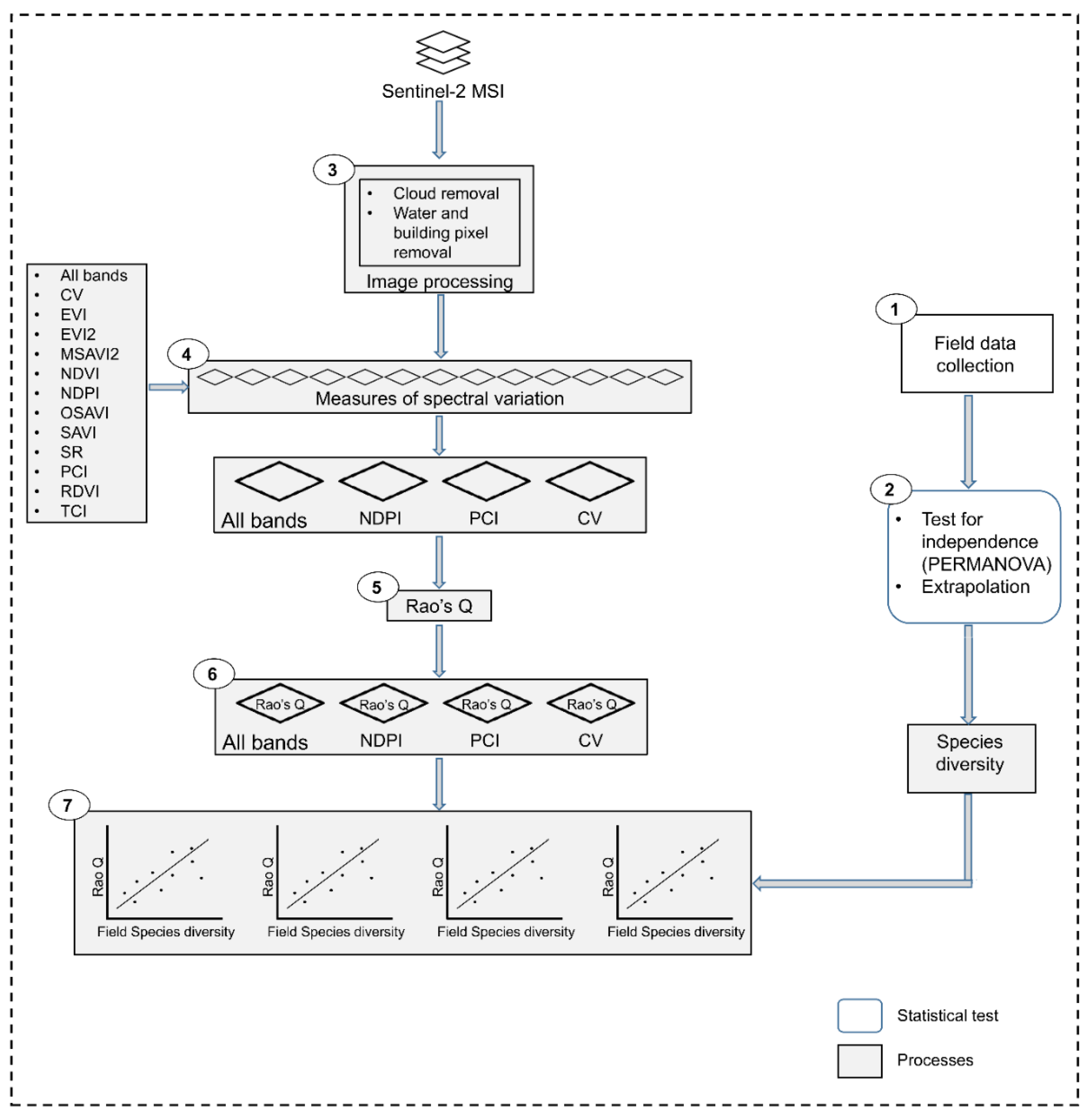
2. Materials and Methods
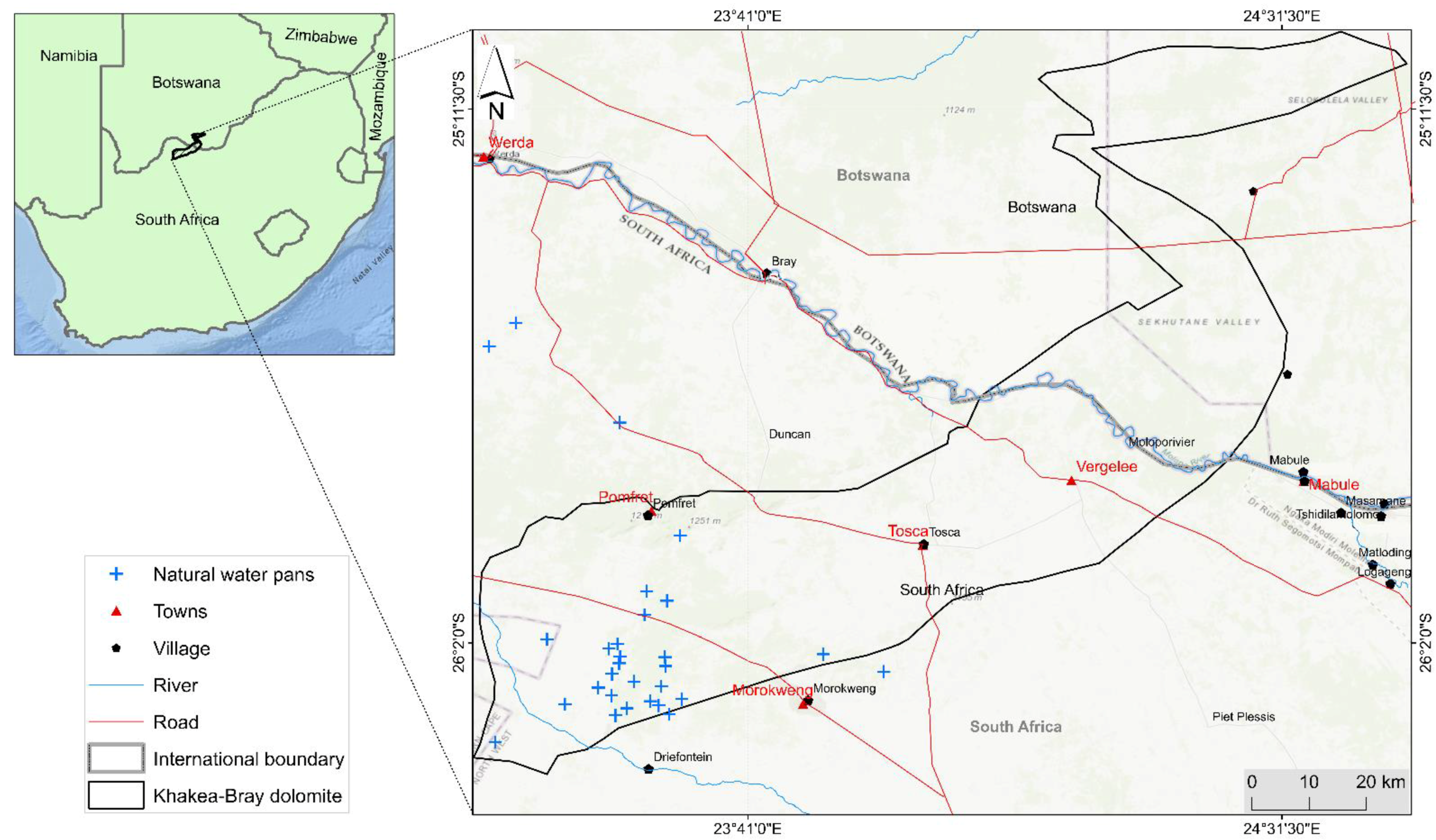
2.1. Study Area

Our study was conducted in the Khakea-Bray (or Pomfret-Vergelegen) TBA. The Khakea-Bray TBA measures ~30,000 km2 and spans across southwestern Botswana and northwestern South Africa (Figure 1). Khakea-Bray TBA is supported by the unconfined and low-yielding Khakea-Bray dolomitic aquifer, which is mainly recharged from precipitation [2,46].
Temperature and rainfall in the Khakea-Bray TBA are characteristic of semi-arid savannah [1,47] with high evapotranspiration rates of 2050–2250 mm/a and low rainfall (300–450 mm) received during the wet season (November–March) [2,46]. Mean temperature ranges from 0 °C to 32 °C and high temperatures are experienced during the dry season (April–October). The climate supports a mixture of Cymbopogon–Themeda veld, bankenveld, and turf thornveld [48].
Figure 1. Map of the Khakea-Bray TBA spanning across Botswana and South Africa. The study is overlaid on baseline topography imagery accessed from ArcMap [49].
Remotesensing 14 02995 g001
Groundwater from the dolomitic aquifer supports different land uses that include agricultural land, wildlife ranching, and communal land [2,45]. In 2002, groundwater was reported to have lowered to 60 m from 20 m due to unsustainable groundwater extraction for agricultural purposes [1,45]. Consequently, the drawdown resulted in the dewatering of the Khakea-Bray TBA dolomitic aquifer supporting several GDEs in the area [45,48]. Upon releasing that the groundwater had lowered, deeper boreholes were sunk and livelihoods dependent on shallower boreholes were affected [1]. Furthermore, groundwater lowering restricted GDV access to the groundwater, putting the ecosystem at risk of invasion by alien plant species [1]. These changes in groundwater are likely to influence the vegetation diversity in the Khakea-Bray TBA (Figure 2).

2.2. Field Campaign and Measuring Vegetation Diversity

Sixteen north-oriented plots were purposively sampled around natural pans (dry and wet) within the Khakea-Bray TBA. Natural water pans are surface depressions filled with rainwater or groundwater seepage [50]. We selected these pans because they were linked to the Khakea-Bray dolomite aquifer which supports all GDEs within this Khakea-Bray ecosystem [45,48]. The natural water pans were considered wet when water was available and dry when there was no water at the water pan. Sampling was done around natural pans since GDEs are more common in these areas owing to the high groundwater level that supports these natural pans [41]. The sampling plots measured 400 m2 (i.e., 20 m × 20 m) and were within 1 km from the natural water pan. The random placement of the plots ensured the plots were at least 100 m away from each other in all directions to avoid biased sampling from autocorrelation. In each sampled plot, we focused on woody and herbaceous plant species composition as well as their corresponding abundance. Notwithstanding the other forms of vegetation physiognomy, grasses and forbes were grouped into one class (i.e., Eragrostis spp.). The species were identified using field guides (e.g., Van Wyk [51]) or with mobile applications (e.g., iNaturalist and PlantSnap). Where the species could not be identified, we took a specimen to the local botanist for identification. The plots were sampled in 2021 during the dry season (June–July). We selected this period since it is characterized by low rainfall, and GDVs are usually productive during the dry period due to access to groundwater. This period also excludes non-GDVs since vegetation dependent on surface water usually dries soon after the wet seasons [3].
To calculate the vegetation diversity for each of the plots, we used the Shannon–Weiner Index (H). H is a commonly used measure and characterizes vegetation diversity based on species richness and evenness [52]. H can be calculated as
H = i = 1 S p i ln p i
where S is the total number of individuals in the plot, and pi is the proportion of species i to S.
However, H is an index of diversity and not in itself diversity [53,54]; hence, H values were converted to the effective number of species (i.e., true diversity) using an exponential function of H. The effective number of species helps one to understand the true diversity of a community [55]. The effective number of species is linear and does not saturate at high values; instead, it accurately provides the number of species that are related to a specific diversity value [53].

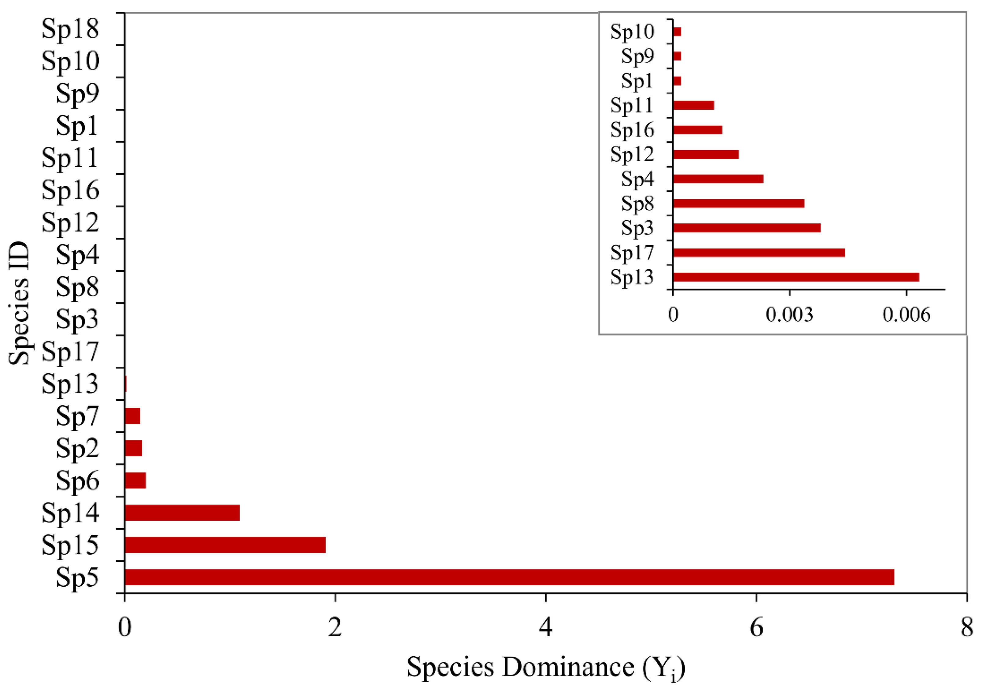
Community Composition and Species Dominance

We used the bootstrapping procedure to extrapolate species richness and estimate the number of unobserved species during our data collection [56]. The technique is nonparametric and estimates species richness from repeated resampling under the assumption of randomness [56]. Bootstrapping was calculated in R, using the vegan package [57] with the following equation:
S e = S o + i = 1 S o ( 1 p i ) N
where Se is the extrapolated species richness, and So is the observed species richness. N is the number of plots, and pi is the frequency of species i.
To test whether there were differences in the species composition of the field-measured data, we used permutational multivariate analysis of variance (PERMANOVA). PERMANOVA tests whether the centroids of dispersion are different between groups [58]. In our study, PERMANOVA tested whether the observed species in each plot were different from the other sampled plots using the Euclidean distance matrices. The distance matrices is calculated iteratively after the geometric partitioning of the plot data on a 2D Euclidean space [59]. The significance of the plot differences was evaluated using the p-value [58]. PERMANOVA was used because it is a robust measure, and our data were not normally distributed based on the Shapiro–Wilk test (p < 0.05). PERMANOVA was run in R using the vegan package with the species composition being the predictor variable and the group (i.e., plot) being the dependent variable.
The dominance index (Y) was used to identify the most dominant species in our sampled plots [60]. Species with Y > 0.02 were considered dominant as compared to all the other species [61,62]. The Y is calculated using the formula
Y i = N i N f i
where Yi is the dominance of species i, and Ni is the abundance of species i. N represents the abundance of all the sampled species, and fi is the frequency of species i.

2.3. Image Acquisition and Processing

Sentinel-2 Multispectral Instrument (MSI) imagery corrected for surface reflectance was accessed through the Google Earth Engine (GEE) platform (https://code.earthengine.google.com (accessed on 10 July 2021)). Surface reflectance data, at 20 m, are provided corrected for geometric and atmospheric errors. The date the image was acquired coincides with the date when our fieldwork was conducted. We also made sure to remove cloud remnants using the mask function in GEE. The Normalized Difference Built-up Index (NDBI) and Modified Normalised Difference Water Index (MNDWI) were also used to mask built-up areas and water, respectively [63,64]. These indices were used due to their robustness in mapping water and built-up areas [63,64]. This was done to avoid the reflectance from built-up areas and water influencing our analysis. Bare surfaces were not removed since these show the absence of vegetation. We used a threshold of ≥0 for NDBI and ≥0 for MNDWI to identify built-up areas and water, respectively. These values were selected based on the literature and our understanding of the study area [63,64].
MNDWI is calculated as
MNDWI = G r e e n S W I R   1 G r e e n + S W I R   1
and NDBI as
NDBI = S W I R   1 N I R S W I R   1 + N I R
where Green, NIR, and SWIR 1 are reflectance regions in the green (B2), near-infrared (B8), and shortwave infrared (B11) from Sentinel-2 MSI, respectively.

2.3.1. Calculating Measures of Spectral Variation

To characterize the vegetation diversity in the Khakea-Bray TBA, we needed to measure the spectral variation in the landscape. We tested 13 measures of spectral variation. These measures include coefficient of variation (CV) [65], Enhanced Vegetation Index (EVI) [66], Enhanced Vegetation Index (EVI) 2 [67], Modified Soil Adjusted Vegetation Index (MSAVI) 2 [68], Normalized Difference Vegetation Index (NDVI) [69], Normalized Difference Phenology Index (NDPI) [70], Optimized Soil Adjusted Vegetation Index (OSAVI) [71], Simple Ratio Index [72], Soil Adjusted Vegetation Index (SAVI) [73], Renormalized Difference Vegetation Index (RDVI) [74], and Tasseled-cap Greenness Index (TCI) [75]. In addition, we also used all the spectral bands from Sentinel-2 MSI and the first principal component of the spectral bands after principal component analysis (PCA). The first principal component accounts for maximum variance and can be a good measure of spectral variation [37,76]. All the other measures included were spectral vegetation indices commonly used in characterizing the spectral heterogeneity in vegetated landscapes [29]. These measures of spectral variation were selected based on their use in SVH studies and how they have been used to characterize landscapes in different environments.

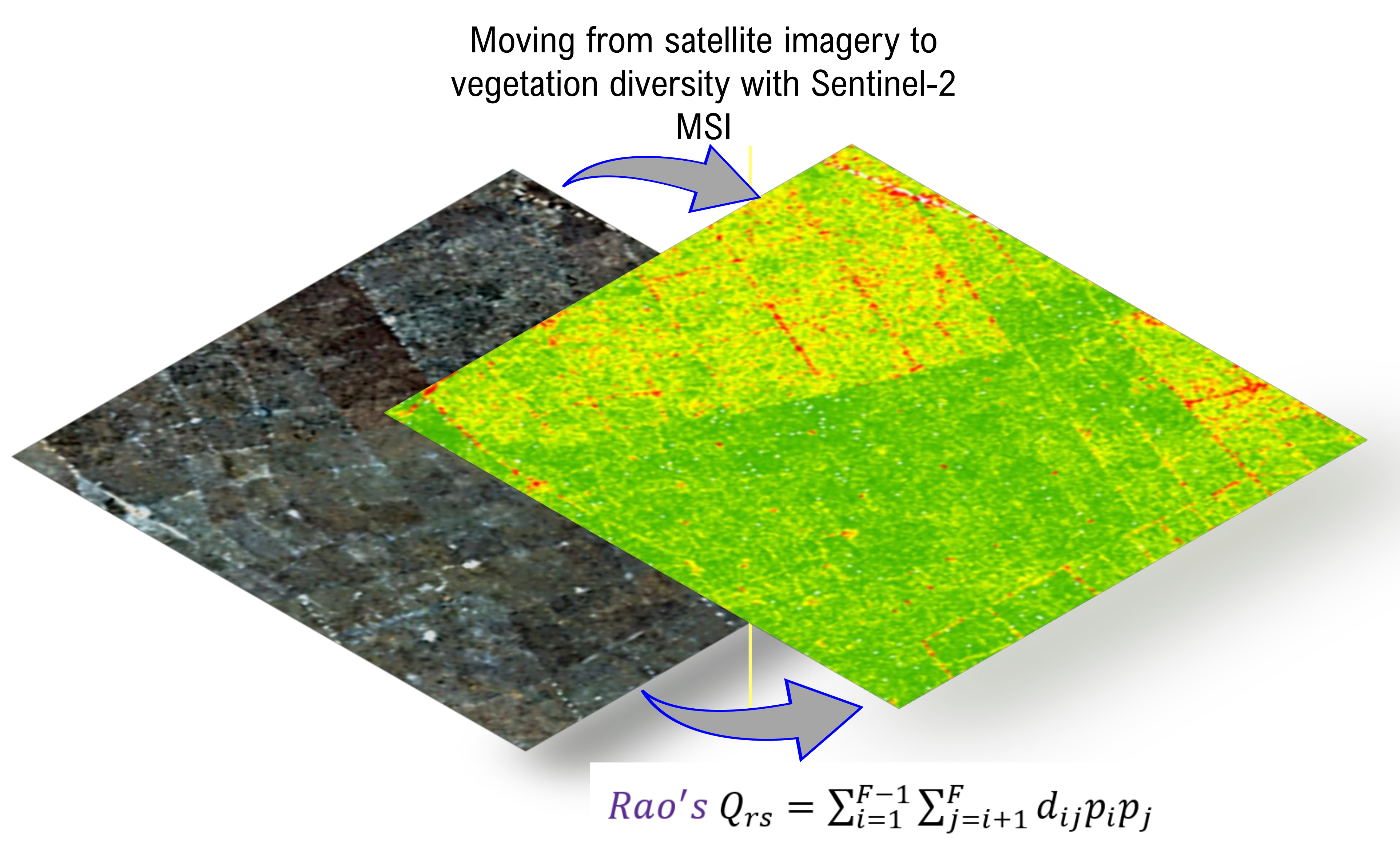
2.3.2. Calculating Vegetation Diversity with the Rao’s Q Using Remote Sensing Data

To measure spectral diversity based on measures of spectral variation, we used the spectral Rao’s Q (hereafter Rao’s Q). The Rao’s Q has been used in studies focusing on the functional diversity of taxa [29,37], and over the last decade, its use in the remote sensing community has increased [29]. Unlike other indices (e.g., Simpson D, Pielou’s evenness, or H) that focus only on the abundance and proportion of species, Rao’s Q also accounts for the distance of the species [29]. Using remote sensing, the Rao’s Q calculates diversity using the pairwise spectral distance between the digital values (DN) of pixel i and j [29]. The Rao’s Q also incorporates the abundance and proportion of pixel i and j. The process is iterative and incorporates all the grids covering the study area. More information on the Rao’s Q can be found in Rocchini, Marcantonio and Ricotta [26]. The Rao’s Q can be calculated as
Q r s = i = 1 F 1 j = i + 1 F d i j p i p j
Qrs represents the Rao Q applied to remote sensing image, and dij is the distance between ith and jth pixel (dij = dji and dii = 0). F is the selected image extent or plot area, with pi and pj being the proportion of pixel i and j to F, respectively.
Rao’s Q was calculated in R [77] for all the measures of spectral variation using a 3 × 3 pixel moving window with the spectralrao function available from Rocchini, Marcantonio and Ricotta [26]. The Rao’s Q was calculated in the classic mode with Euclidean distance.
The Rao’s Q calculated from Enhanced Vegetation Index (EVI), Enhanced Vegetation Index (EVI) 2, Modified Soil Adjusted Vegetation Index (MSAVI) 2, Normalized Difference Vegetation Index (NDVI), Optimized Soil Adjusted Vegetation Index (OSAVI), Simple Ratio Index (SR), Soil Adjusted Vegetation Index (SAVI), Renormalized Difference Vegetation Index (RDVI), and Tasseled-cap Greenness Index (TCI) returned zero for more than 50% of the study area; hence, results from these indices were not considered. The Rao’s Q computes pairwise differences and returns zero when the pairwise difference of the digital numbers (DN) from the measures of spectral variation is zero [26,37].

2.3.3. Evaluating Remote Sensing-Derived Diversity

We used the coefficient of determination (R2) at the 95% confidence interval to examine the linear relationship between remote sensing-derived diversity (i.e., Rao’s Q) and field-measured diversity (i.e., the effective number of species). R2 was used to examine the proportion of the variance between the Rao’s Q and the field-measured diversity. The R2 was calculated for all the Rao’s Q metrics derived from the four measures of spectral variation. R2 was executed in R. We summarize the entire methods section in Figure 3.

2.3.4. Effect of Distance from the Natural Water Pan on Vegetation Diversity

The best-performing measure of spectral variation was then selected to test the variation of Rao’s Q with increasing distance from the natural pans. This was tested for dry and wet natural pans in the study area. To measure the distance, we created non-overlapping buffers around the natural pans and derived the corresponding Rao’s Q using zonal statistics in ArcMap 10.8 [49]. Curve estimation techniques were used to evaluate the relationship between distance from the natural pan and the corresponding Rao’s Q. To achieve this, we ran six regression models (i.e., linear, cubic, quadratic, inverse, logarithmic, and polynomial) and evaluated them using the corrected Akaike Information Criterion (AICc) for the wet and dry natural pans. The AIC is an estimator of model error, and a model with a lower AIC is better as compared to a model with a higher AIC [78]. In addition, AIC penalizes models for using more variables, hence balancing model fitness and model simplicity pans [78]. The AICc was used instead of the AIC since the AICc is corrected for small sample sizes. Lastly, the Student’s t-test [79] was used to test and describe the mean difference in the Rao’s Q between the dry or wet natural pans.

3. Results

3.1. Species Composition, Diversity, and Dominance

From the sampled plots, 18 plant species were observed in the field (Supplementary Table S1), and bootstrap extrapolation showed that at least 3.56 species were unseen. In addition, amongst the sampled plots, the PERMANOVA showed that species composition did not significantly differ (p = 0.79) (Supplementary Table S2). We also observed that vegetation diversity (effective number of species) varied within the sampled plots. Most of the plots had low vegetation diversity (<2.5) with only a few plots with high vegetation diversity (>3).
Of the observed plant species, Eragrostis spp. was the most dominant species (Dominance index = 7.3), followed by Senegalia nigrescens (Dominance index = 1.91), Scorzonera humilis (Dominance index = 1.09), and Leonotis ocymifolia (Dominance index = 0.20) (Figure 4). Rare species that were less dominant were also observed within the sampled plots, and these include Ziziphus mucronate, Leucas martinicensis, and Lipia javani.

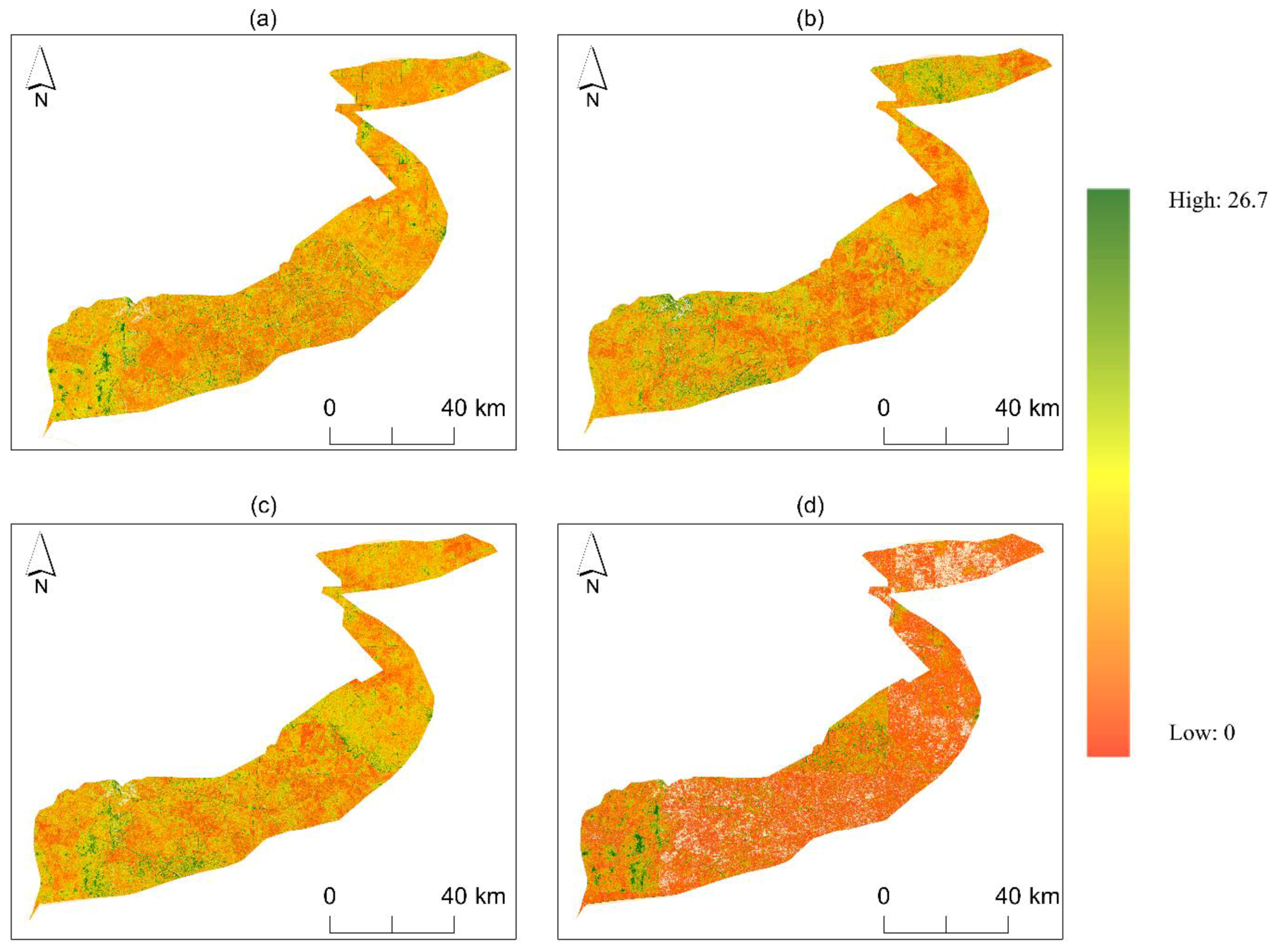
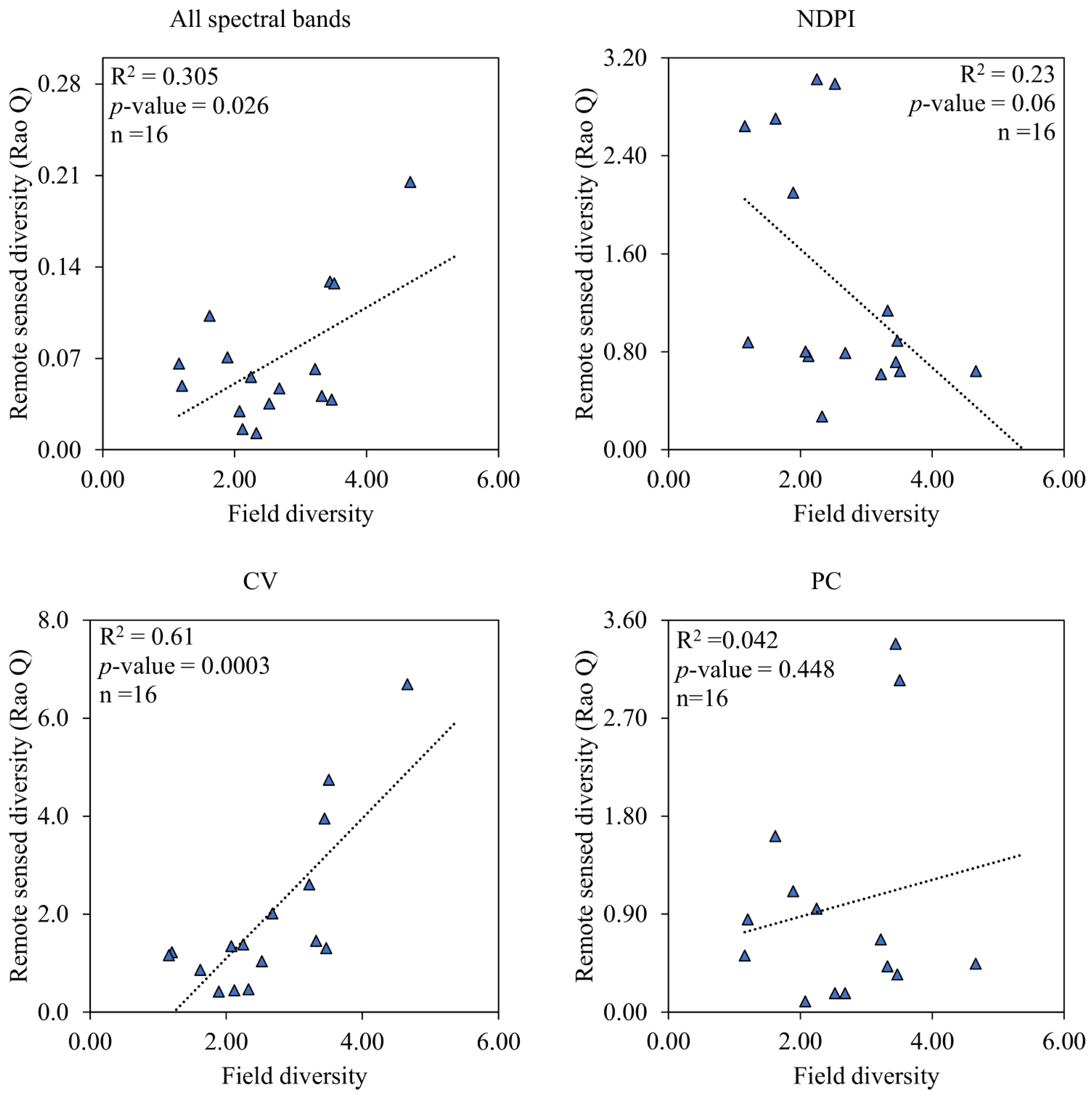
3.2. Distribution and Performance of Spectral Diversity from Remote Sensing Data

Using qualitative analysis, remotely sensed diversity (Rao’s Q) derived from measures of spectral variation was observed to be higher in the southwestern part of the study area. Specifically, vegetation diversity was highest around natural water pans and along fence lines, roads, and rivers (Figure 5). In other parts of the study area, the Rao’s Q was either low or intermediate, and this was typically in grassland or cultivated areas. High spatial fidelity was observed when all the spectral bands were used and from the coefficient of variation. On the other hand, the NDPI and principal component had low spatial fidelity.
The coefficient of determination showed that vegetation diversity measured from remote sensing data was related to field data (R2 > 0.01). Association between field-measured vegetation diversity and the Rao’s Q was significantly high for the coefficient of variation and the reflectance of all the spectral bands (R2 > 0.3 and p < 0.05) (Figure 6). However, the Normalised Difference Phenology Index and the first principal component did not exhibit high association.

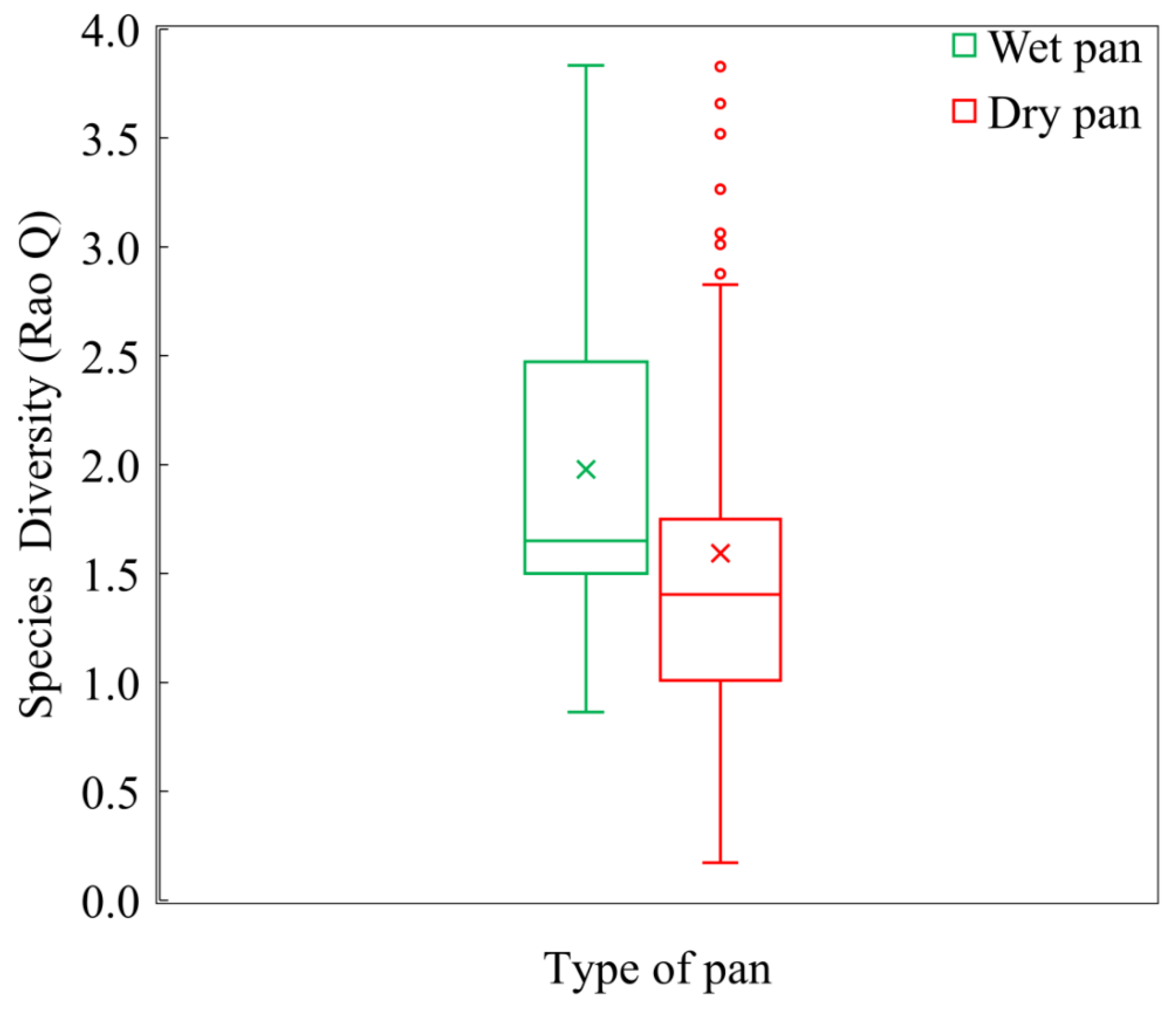
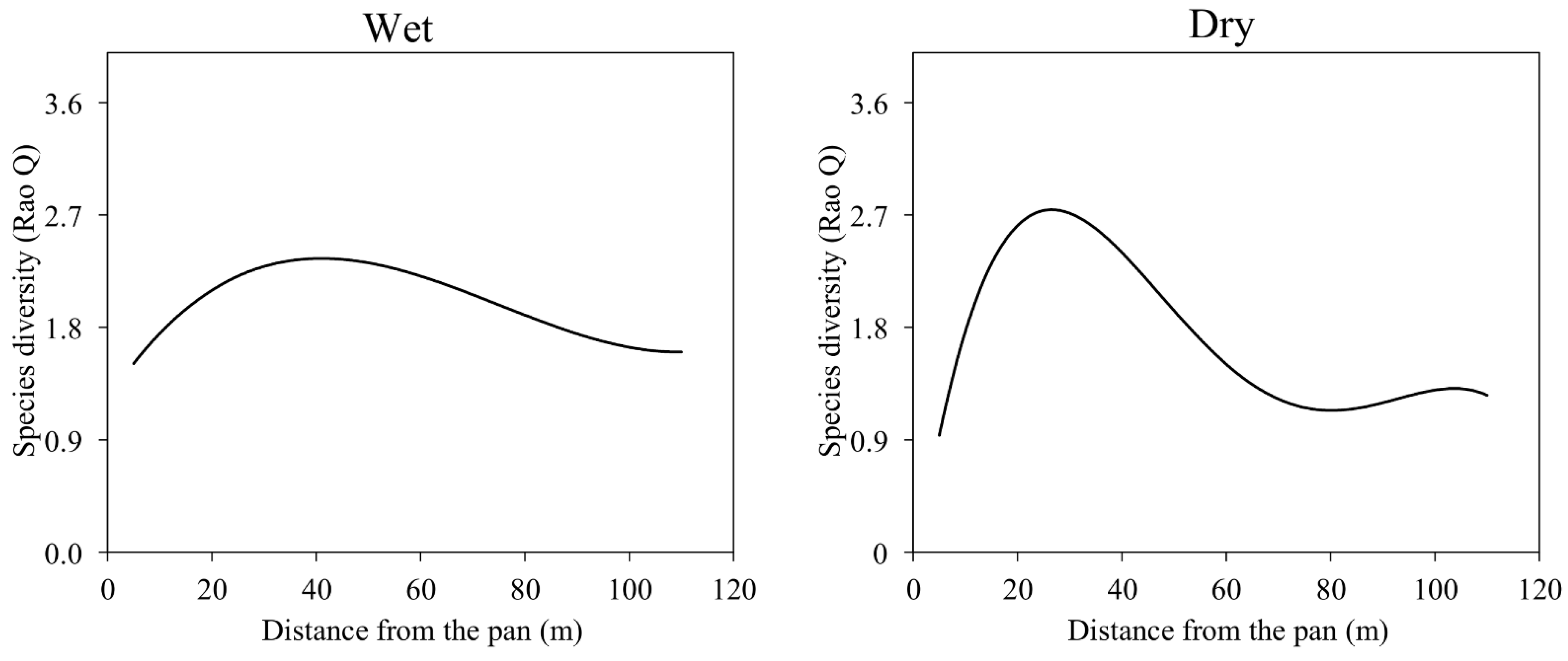
3.3. Vegetation Diversity and Distance from the Natural Pan

Using curve estimation techniques, we observed that vegetation diversity around dry and wet natural pans was related to distance from the natural pans. The logarithmic equation explained the relationship between vegetation diversity and distance from the pans for the wet and dry natural water pans (Table 1). The vegetation diversity (Rao’s Q) between the wet and dry natural pans was also observed not to differ significantly (p > 0.05) (Figure 7).
Our results showed that vegetation diversity decreased with increasing distance from the natural pan (Figure 8). The decrease in vegetation diversity around wet natural pans was gradual and only peaked at ~40 m. However, vegetation diversity around dry natural pans peaked at ~25 m and sharply dropped afterward with increasing distance.

4. Discussion

In this study, we used Sentinel-2 MSI to test whether the Rao’s Q could be used to characterize vegetation diversity in groundwater-dependent ecosystems (GDEs) within the Khakea-Bray TBA.

4.1. Species Composition and the Performance of Measures of Spectral Variation in Estimating Vegetation Diversity

We found out that species composition did not significantly vary amongst all the sampled plots in the Khakea-Bray TBA. The Khakea-Bray TBA is likely a homogenous environment since it is mainly dominated by a few vegetation species. This was supported by our observations of how only four plant species (Eragrostis spp., Senegalia nigrescens, Scorzonera humilis, and Leonotis ocymifolia) dominated the area under study. The dominant vegetation types are common in the Khakea-Bray TBA, since it is mainly characterized by the Molopo Bushveld, Mafikeng Bushveld, and Kuruman Mountain Bushveld (Spickett et al., 2011; Van Dyk, 2005; Mucina and Rutherford, 2006). The dominant vegetation species observed in the study area are likely to be the facultative phreatophytes (i.e., will use groundwater when it is available) and will outcompete other species that are obligatory phreatophytes or non-groundwater-dependent within the Khakea-Bray TBA. Our observations are supported by the niche differentiation concept, which postulates that a heterogeneous environment likely has more species as compared to a homogeneous environment [80,81].
Leaf structural and chemical properties usually drive the spectral heterogeneity observed in vegetation spectral reflectance [76]. The low performance of the Normalized Difference Phenology Index and the first principal component in estimating the Rao’s Q can be explained by how these metrics capture spectral heterogeneity more in vegetated landscapes than in arid environments with intense soil reflectance [70,82]. In addition, these measures might be more sensitive to a specific component of diversity (i.e., evenness, abundance, or dominance) [65,83]. Henceforth, these metrics might perform better in areas with high environmental heterogeneity (e.g., temperate forests) or with a different measure of diversity [76,84].
The Rao’s Q estimated from the coefficient of variation (CV) performed better than the Rao’s Q estimated from all the other measures of spectral variation. In this study, CV was used to measure the variability in spectral reflectance amongst pixels from all the spectral bands [27,84]. CV is highly sensitive to the reflectance of rare and abundant species and is a good measure of spectral variation [65,84]. The CV has been used in different studies [27,37,65], focusing on monitoring different aspects of the environment [85,86]. Owing to its ability for detecting spectral heterogeneity, the high performance of the CV over other measures of spectral variation is expected [65,85].

4.2. Distribution of Vegetation Diversity in the Khakea-Bray TBA

We observed that vegetation diversity, measured with the Rao’s Q, was highest around natural water pans and along rivers and roads. Groundwater from the Khakea-Bray dolomitic aquifer discharges into natural water pans and rivers, and this facilitates the presence of high vegetation diversity along and around these areas [1,44,48]. In addition, groundwater is usually enriched as it flows through different soils, and some of these nutrients improve plant growth [87]. Consequently, around natural water pans and along rivers (i.e., riparian zone), species compete for nutrients and water availability from access to groundwater. This is true since soil moisture and fertility are limiting factors to plant growth in other parts of our study area where vegetation diversity was low. Just as competitive exclusion explains the low diversity in other parts of our study areas, niche partitioning might be responsible for the high vegetation diversity around natural water pans and along rivers [88].
As the groundwater level deepens, species competition will likely change, and vegetation diversity will lower. This phenomenon is supported by our observations of how vegetation diversity decreased with increasing distance from the natural water pans, thus resembling an inverse piosphere. The inverse piospheric response of vegetation diversity around natural water pans means there is minimal utilization or grazing of vegetation around natural water pans [89]. The minimal grazing or utilization of vegetation by livestock around natural water pans gives them a selective advantage over other vegetation species, thus allowing the vegetation diversity to be high around natural water pans [88]. The minimal utilization explained by the piosphere effect could also be responsible for the minimal difference in the species diversity between the dry and wet natural water pans. Our observations of high vegetation diversity around natural water pans and along rivers are coherent with previous work on how vegetation diversity lowers with decreasing groundwater depth [88,90,91].
Our results also showed that non-groundwater-dependent areas had high vegetation diversity. Specifically, this was observed along roads and fence lines. Roads are dispersal corridors [92] with high propagule pressure from the constant disturbance during maintenance and construction [93]. The constant disturbance changes the soil properties and improves soil fertility (i.e., from the increased decomposition of nutrients) [94,95]. The improved soil fertility facilitates the colonization of roads by synanthropic plant species (specifically ruderal apophytes) that can quickly establish themselves and therefore increase the vegetation diversity along roads [95,96]. This explains our observations of the dominance of Eragrostis spp., since the species can easily invade and establish itself along roadsides [97,98]. On the other hand, our observation of high species diversity along fence lines could plausibly be related to the community preference of using mixed element fences that consist of living and non-living posts. Mixed element fences consist of plant species that can easily resprout and require minimal attention [99]. In addition, posts for mixed element fences are from several tree species for extra strength, thus influencing the vegetation diversity along the fence line [100].
The SVH does not hold in all environments [32], but its applicability has been tested with success in several environments including alpine conifers [37] and grasslands [101]. Our study presents the first attempt to utilize the Rao’s Q in characterizing species diversity in GDEs within an arid environment. Findings from this study are supported by empirical data from field-measured diversity, which explained at least 61% of the remote sensing-derived vegetation diversity (Rao’s Q). When compared to other studies—for example, Madonsela, Cho, Ramoelo and Mutanga [83]; Madonsela, Cho, Ramoelo and Mutanga [65]; Rocchini, Chiarucci and Loiselle [25]; and Lopes, Fauvel, Ouin and Girard [101]—our observations are more robust. For example, Madonsela, Cho, Ramoelo and Mutanga [83] and Rocchini, Chiarucci and Loiselle [25] reported a low R2 (0–0.48) when explaining vegetation diversity in South Africa and Italy, respectively. Our findings are also credible since we calculate the Rao’s Q from several measures of spectral variation, as opposed to other studies that only used single measures such as the principal components [76], NDVI [83], or CV [65]. The applicability of the SVH strongly relies on the measures of spectral variation used, and the measure should be able to detect subtle differences in vegetation spectral reflectance with either medium- or low-resolution sensors [29]. In light of this understanding, our study used 13 spectral indices in measuring the spectral variation of vegetation diversity. However, nine of the spectral indices assumed our study environment was homogenous and thus returned zero values for more than 50% of the study area. Although these measures of spectral variation have performed well in other environments, their use in arid environments remains limited. Future studies might consider using environment-specific measures of spectral variation.
The temporal variation in vegetation phenology might have also influenced our results when detecting spectral heterogeneity since we used a single image and not multi-temporal images. Caution should also be taken when interpreting our results since some of the areas within the Khakea-Bray TBA are not groundwater-dependent. This is regardless of how these areas might have high or low vegetation diversity. Future studies using the Rao’s Q can test it with data from multi-temporal high-resolution imagery.

4.3. Implications of Using Vegetation Diversity on Monitoring and Conserving GDE

There exists limited knowledge on biodiversity globally (i.e., Linnean shortfall), and environments without ecological or economic significance are rarely prioritized in conservation programs regardless of the associated Sustainable Development Goals (SDG) [102]. This approach has led to the degradation of many GDEs since their significance was not realized in time [4,103]. Although conservation is costly, identifying priority conservation areas can assist in the management of ecosystems at risk of degradation [104]. Although this approach is economically sound, it might put other ecosystems at risk [102,104]. Our methodology and results provide resource managers and ecologists with a framework for characterising and identifying priority conservation areas where a priori information does not exist. Using the SVH and remotely sensed data can provide resource managers insights into the vegetation diversity in the Khakea-Bray TBA, and they can use this as a proxy for identifying priority areas that need to be conserved or monitored for invasive species.

5. Conclusions

Understanding vegetation diversity in GDEs is pivotal to the management or conservation of the Khakea-Bray TBA. Currently, field techniques are costly, and more innovative and accurate ways capable of providing us knowledge about vegetation diversity in GDEs are sought. Our study presents the first attempt to characterize vegetation diversity in the transboundary aquifer that is under threat from climate change and anthropogenic activities. We provide evidence on how the Rao’s Q can be used with Sentinel-2 MSI to characterize and provide the vegetation diversity for GDEs within the Khakea-Bray TBA. This work also allows for the identification of priority conservation areas in the Khakea-Bray TBA. Our work provides resource managers with a pathway towards achieving national and regional Aichi biodiversity targets as well as SDG 15. Therefore, future studies can use our methodology in providing a priori knowledge about all global ecosystems including GDEs.

Supplementary Materials

The following supporting information can be downloaded at: https://www.mdpi.com/article/10.3390/rs14132995/s1, Table S1: Species inventory of all the species that were observed when sampling the field plots; Table S2: PERMANOVA results from comparing the difference in species composition amongst the sampled plots, where Df is the degrees of freedom, SumsOfSqs is the sum of squares, MeanSqs represents the mean sum of squares, and F.Model is the pseudo F-ratio. R2 is the coefficient of determination, and Pr(>F) is the significance at the 95% confidence interval.

Author Contributions

K.S.M.: Conceptualization, Methodology, Writing—Original Draft Preparation, Writing—Reviewing and Editing. T.D. (Timothy Dube): Conceptualization, Supervision, Writing—Reviewing and Editing. F.D.: Supervision, Software, Validation. T.D. (Tatenda Dalu): Conceptualization, Supervision, Methodology, Writing—Reviewing and Editing. All authors have read and agreed to the published version of the manuscript.

Funding

The authors received support from the Southern African Development Community (SADC) Groundwater Management Institute (GMI) through a grant from the JRS Biodiversity Foundation.

Data Availability Statement

Data used in this research are freely available online and upon request.

Acknowledgments

The authors are grateful for the support offered by JRS Biodiversity Foundation through the Southern African Development Community (SADC) Groundwater Management Institute (GMI). The authors would also like to extend their gratitude to the anonymous reviewers who improved the manuscript.

Conflicts of Interest

The authors declare that there exist no competing financial interest or personal relationships that could have appeared to influence the work reported in this study.

References

  1. Seward, P.; van Dyk, G.S.d.T. Turning the tide–curbing groundwater over-abstraction in the Tosca-Molopo area, South Africa. In Advances in Groundwater Governance; Villholth, K.G., López-Gunn, E., Conti, K., Eds.; CRC Press: Boca Raton, FL, USA, 2018; pp. 511–525. [Google Scholar]
  2. Turton, A.; Godfrey, L.; Julien, F.; Hattingh, H. Unpacking Groundwater Governance through the Lens of a Trialogue: A Southern African Case Study. In Proceedings of the International Symposium on Groundwater Sustainability (ISGWAS), Alicante, Spain, 23–27 January 2006; pp. 24–27. [Google Scholar]
  3. Eamus, D.; Fu, B.; Springer, A.E.; Stevens, L.E. Groundwater dependent ecosystems: Classification, identification techniques and threats. In Integrated Groundwater Management: Concepts, Approaches and Challenges; Jakeman, A.J., Barreteau, O., Hunt, R.J., Rinaudo, J.-D., Ross, A., Eds.; Springer International Publishing: Cham, Switzerland, 2016; pp. 313–346. [Google Scholar]
  4. Murray, B.R.; Hose, G.C.; Eamus, D.; Licari, D. Valuation of groundwater-dependent ecosystems: A functional methodology incorporating ecosystem services. Aust. J. Bot. 2006, 54, 221–229. [Google Scholar] [CrossRef]
  5. Sousa, M.R.; Rudolph, D.L.; Frind, E.O. Threats to groundwater resources in urbanizing watersheds: The waterloo moraine and beyond. Can. Water Resour. J. Rev. Can. Des Ressour. Hydr. 2014, 39, 193–208. [Google Scholar] [CrossRef]
  6. Wu, W.-Y.; Lo, M.-H.; Wada, Y.; Famiglietti, J.S.; Reager, J.T.; Yeh, P.J.F.; Ducharne, A.; Yang, Z.-L. Divergent effects of climate change on future groundwater availability in key mid-latitude aquifers. Nat. Commun. 2020, 11, 3710. [Google Scholar] [CrossRef]
  7. Clifton, C.; Evans, R.; Hayes, S.; Hirji, R.; Puz, G.; Pizarro, C. Water and Climate Change: Impacts on Groundwater Resources and Adaptation Options; World Bank: Washington, DC, USA, 2010. [Google Scholar]
  8. Kreamer, D.K.; Stevens, L.E.; Ledbetter, J.D. Groundwater dependent ecosystems—Science, challenges, and policy directions. Groundwater 2015, 205, 230. [Google Scholar]
  9. Kløve, B.; Ala-Aho, P.; Bertrand, G.; Gurdak, J.J.; Kupfersberger, H.; Kværner, J.; Muotka, T.; Mykrä, H.; Preda, E.; Rossi, P. Climate change impacts on groundwater and dependent ecosystems. J. Hydrol. 2014, 518, 250–266. [Google Scholar] [CrossRef]
  10. Alaibakhsh, M.; Emelyanova, I.; Barron, O.; Khiadani, M.; Warren, G. Large-scale regional delineation of riparian vegetation in the arid and semi-arid Pilbara region, WA. Hydrol. Process. 2017, 31, 4269–4281. [Google Scholar] [CrossRef]
  11. Pengra, B.W.; Johnston, C.A.; Loveland, T.R. Mapping an invasive plant, Phragmites australis, in coastal wetlands using the eo-1 hyperion hyperspectral sensor. Remote Sens. Environ. 2007, 108, 74–81. [Google Scholar] [CrossRef]
  12. Xu, C.; Holmgren, M.; Van Nes, E.H.; Maestre, F.T.; Soliveres, S.; Berdugo, M.; Kéfi, S.; Marquet, P.A.; Abades, S.; Scheffer, M. Can we infer plant facilitation from remote sensing? A test across global drylands. Ecol. Appl. 2015, 25, 1456–1462. [Google Scholar] [CrossRef] [Green Version]
  13. Lv, J.; Wang, X.S.; Zhou, Y.; Qian, K.; Wan, L.; Eamus, D.; Tao, Z. Groundwater-dependent distribution of vegetation in Hailiutu river catchment, a semi-arid region in China. Ecohydrology 2013, 6, 142–149. [Google Scholar] [CrossRef]
  14. Barron, O.V.; Emelyanova, I.; Van Niel, T.G.; Pollock, D.; Hodgson, G. Mapping groundwater-dependent ecosystems using remote sensing measures of vegetation and moisture dynamics. Hydrol. Process. 2014, 28, 372–385. [Google Scholar] [CrossRef]
  15. De Klerk, A.; De Klerk, L.; Oberholster, P.; Ashton, P.; Dini, J.; Holness, S. A Review of Depressional Wetlands (Pans) in South Africa, Including a Water Quality Classification System; WRC Report No 2230/1/16; Water Research Commission: Gezina, South Africa, 2016. [Google Scholar]
  16. Eamus, D.; Froend, R.; Loomes, R.; Hose, G.; Murray, B. A functional methodology for determining the groundwater regime needed to maintain the health of groundwater-dependent vegetation. Aust. J. Bot. 2006, 54, 97–114. [Google Scholar] [CrossRef] [Green Version]
  17. Orellana, F.; Verma, P.; Loheide, S.P.; Daly, E. Monitoring and modeling water-vegetation interactions in groundwater-dependent ecosystems. Rev. Geophys. 2012, 50, RG3003. [Google Scholar] [CrossRef]
  18. Eamus, D.; Froend, R. Groundwater-dependent ecosystems: The where, what and why of gdes. Aust. J. Bot. 2006, 54, 91–96. [Google Scholar] [CrossRef]
  19. Chiloane, C.; Dube, T.; Shoko, C. Impacts of groundwater and climate variability on terrestrial groundwater dependent ecosystems: A review of geospatial assessment approaches and challenges and possible future research directions. Geocarto Int. 2021. [Google Scholar] [CrossRef]
  20. John, R.; Chen, J.; Lu, N.; Guo, K.; Liang, C.; Wei, Y.; Noormets, A.; Ma, K.; Han, X. Predicting plant diversity based on remote sensing products in the semi-arid region of inner mongolia. Remote Sens. Environ. 2008, 112, 2018–2032. [Google Scholar] [CrossRef]
  21. Li, X.; Chen, W.; Cheng, X.; Liao, Y.; Chen, G. Comparison and integration of feature reduction methods for land cover classification with rapideye imagery. Multimed. Tools Appl. 2017, 76, 23041–23057. [Google Scholar] [CrossRef]
  22. Woods, J.; Sekhwela, M.B.M. The vegetation resources of botswana’s savannas: An overview. S. Afr. Geogr. J. 2003, 85, 69–79. [Google Scholar] [CrossRef]
  23. Rocchini, D.; Ricotta, C.; Chiarucci, A. Using satellite imagery to assess plant species richness: The role of multispectral systems. Appl. Veg. Sci. 2007, 10, 325–331. [Google Scholar] [CrossRef]
  24. Nagendra, H.; Gadgil, M. Satellite imagery as a tool for monitoring species diversity: An assessment. J. Appl. Ecol. 1999, 36, 388–397. [Google Scholar] [CrossRef]
  25. Rocchini, D.; Chiarucci, A.; Loiselle, S.A. Testing the spectral variation hypothesis by using satellite multispectral images. Acta Oecologica 2004, 26, 117–120. [Google Scholar] [CrossRef]
  26. Rocchini, D.; Marcantonio, M.; Ricotta, C. Measuring Rao’s Q diversity index from remote sensing: An open source solution. Ecol. Indic. 2017, 72, 234–238. [Google Scholar] [CrossRef]
  27. Wang, R.; Gamon, J.A.; Emmerton, C.A.; Li, H.; Nestola, E.; Pastorello, G.Z.; Menzer, O. Integrated analysis of productivity and biodiversity in a southern alberta prairie. Remote Sens. 2016, 8, 214. [Google Scholar] [CrossRef] [Green Version]
  28. Wang, R.; Gamon, J.A. Remote sensing of terrestrial plant biodiversity. Remote Sens. Environ. 2019, 231, 111218. [Google Scholar] [CrossRef]
  29. Torresani, M.; Feilhauer, H.; Rocchini, D.; Féret, J.-B.; Zebisch, M.; Tonon, G. Which optical traits enable an estimation of tree species diversity based on the spectral variation hypothesis? Appl. Veg. Sci. 2021, 24, e12586. [Google Scholar] [CrossRef]
  30. Nagendra, H.; Rocchini, D.; Ghate, R.; Sharma, B.; Pareeth, S. Assessing plant diversity in a dry tropical forest: Comparing the utility of landsat and ikonos satellite images. Remote Sens. 2010, 2, 478–496. [Google Scholar] [CrossRef] [Green Version]
  31. Cavender-Bares, J.; Schweiger, A.K.; Pinto-Ledezma, J.N.; Meireles, J.E. Applying remote sensing to biodiversity science. In Remote Sensing of Plant Biodiversity; Springer: Cham, Switzerland, 2020; pp. 13–42. [Google Scholar]
  32. Schmidtlein, S.; Fassnacht, F.E. The spectral variability hypothesis does not hold across landscapes. Remote Sens. Environ. 2017, 192, 114–125. [Google Scholar] [CrossRef] [Green Version]
  33. Mandanici, E.; Bitelli, G. Preliminary comparison of sentinel-2 and landsat 8 imagery for a combined use. Remote Sens. 2016, 8, 1014. [Google Scholar] [CrossRef] [Green Version]
  34. Rocchini, D. Effects of spatial and spectral resolution in estimating ecosystem α-diversity by satellite imagery. Remote Sens. Environ. 2007, 111, 423–434. [Google Scholar] [CrossRef]
  35. Gould, W. Remote sensing of vegetation, plant species richness, and regional biodiversity hotspots. Ecol. Appl. 2000, 10, 1861–1870. [Google Scholar] [CrossRef]
  36. Dahlin, K.M. Spectral diversity area relationships for assessing biodiversity in a wildland–agriculture matrix. Ecol. Appl. 2016, 26, 2758–2768. [Google Scholar] [CrossRef] [PubMed]
  37. Torresani, M.; Rocchini, D.; Sonnenschein, R.; Zebisch, M.; Marcantonio, M.; Ricotta, C.; Tonon, G. Estimating tree species diversity from space in an alpine conifer forest: The Rao’s Q diversity index meets the spectral variation hypothesis. Ecol. Inform. 2019, 52, 26–34. [Google Scholar] [CrossRef] [Green Version]
  38. Fisher, M.C.; Henk, D.A.; Briggs, C.J.; Brownstein, J.S.; Madoff, L.C.; McCraw, S.L.; Gurr, S.J. Emerging fungal threats to animal, plant and ecosystem health. Nature 2012, 484, 186–194. [Google Scholar] [CrossRef]
  39. Ayyad, M.A. Case studies in the conservation of biodiversity: Degradation and threats. J. Arid. Environ. 2003, 54, 165–182. [Google Scholar] [CrossRef] [Green Version]
  40. Bongaarts, J. IPBES, 2019. Summary for policymakers of the global assessment report on biodiversity and ecosystem services of the intergovernmental science-policy platform on biodiversity and ecosystem services. Popul. Dev. Rev. 2019, 45, 680–681. [Google Scholar] [CrossRef] [Green Version]
  41. Brown, J.; Wyers, A.; Aldous, A.; Bach, L. Groundwater and Biodiversity Conservation: A Methods Guide for Integrating Groundwater Needs of Ecosystems and Species into Conservation Plans in the Pacific Northwest; The Nature Conservancy: Portland, OR, USA, 2007. [Google Scholar]
  42. Eales, K. Equity and Efficiency in Water Services: The Climate Change Dimension; Water Institute of Southern Africa: Midrand, South Africa, 2010. [Google Scholar]
  43. Davies, J.; Robins, N.S.; Farr, J.; Sorensen, J.; Beetlestone, P.; Cobbing, J.E. Identifying transboundary aquifers in need of international resource management in the southern african development community region. Hydrogeol. J. 2013, 21, 321–330. [Google Scholar] [CrossRef] [Green Version]
  44. Ngobe, T. Investigation of Groundwater Discharge Processes in GDEs in the Khakea Bray Transboundary Aquifer. 2021. Available online: https://sadc-gmi.org/wp-content/uploads/2021/08/SADC-JRS-project-presentation-Thandeka.pdf (accessed on 15 November 2021).
  45. Godfrey, L.; van Dyk, G. Reserve Determination for the Pomfret-Vergelegen Dolomitic Aquifer, North West Province, Part of Catchments D41C, D, E and F; CSIR Report Env-P-C; CSIR: Pretoria, South Africa, 2002. [Google Scholar]
  46. Altchenko, Y.; Villholth, K.G. Transboundary aquifer mapping and management in africa: A harmonised approach. Hydrogeol. J. 2013, 21, 1497–1517. [Google Scholar] [CrossRef]
  47. Nijsten, G.-J.; Christelis, G.; Villholth, K.G.; Braune, E.; Gaye, C.B. Transboundary aquifers of africa: Review of the current state of knowledge and progress towards sustainable development and management. J. Hydrol. Reg. Stud. 2018, 20, 21–34. [Google Scholar] [CrossRef]
  48. Van Dyk, G.S.D.T. Managing the Impact of Irrigation on the Tosca-Molopo Groundwater Resource. Ph.D. Thesis, University of the Free State, Bloemfontein, South Africa, 2005. [Google Scholar]
  49. Environmental Systems Research Institute. Arcgis 10.8; Environmental Systems Research Institute: Redlands, CA, USA, 2020. [Google Scholar]
  50. Arendt, R.; Reinhardt-Imjela, C.; Schulte, A.; Faulstich, L.; Ullmann, T.; Beck, L.; Martinis, S.; Johannes, P.; Lengricht, J. Natural pans as an important surface water resource in the Cuvelai basin—metrics for storage volume calculations and identification of potential augmentation sites. Water 2021, 13, 177. [Google Scholar] [CrossRef]
  51. Van Wyk, B. Field Guide to Trees of Southern Africa; Penguin Random House South Africa: Cape Town, South Africa, 2013. [Google Scholar]
  52. Jost, L. The relation between evenness and diversity. Diversity 2010, 2, 207–232. [Google Scholar] [CrossRef]
  53. Jost, L. Entropy and diversity. Oikos 2006, 113, 363–375. [Google Scholar] [CrossRef]
  54. Chao, A.; Gotelli, N.J.; Hsieh, T.; Sander, E.L.; Ma, K.; Colwell, R.K.; Ellison, A.M. Rarefaction and extrapolation with hill numbers: A framework for sampling and estimation in species diversity studies. Ecol. Monogr. 2014, 84, 45–67. [Google Scholar] [CrossRef] [Green Version]
  55. Chao, A.; Chiu, C.-H.; Jost, L. Unifying species diversity, phylogenetic diversity, functional diversity, and related similarity and differentiation measures through hill numbers. Annu. Rev. Ecol. Evol. Syst. 2014, 45, 297–324. [Google Scholar] [CrossRef] [Green Version]
  56. Smith, E.P.; van Belle, G. Nonparametric estimation of species richness. Biometrics 1984, 40, 119–129. [Google Scholar] [CrossRef] [Green Version]
  57. Oksanen, J.; Kindt, R.; Legendre, P.; O’Hara, B.; Stevens, M.H.H.; Oksanen, M.J.; Suggests, M. The vegan package. Community Ecol. Package 2007, 10, 719. [Google Scholar]
  58. Anderson, M.J. A new method for non-parametric multivariate analysis of variance. Austral Ecol. 2001, 26, 32–46. [Google Scholar]
  59. Anderson, M.J. Permutational Multivariate Analysis of Variance (PERMANOVA); John Wiley & Sons, Ltd.: Hoboken, NJ, USA, 2017; pp. 1–15. [Google Scholar]
  60. Guo, C.; Zhu, G.; Qin, B.; Zhang, Y.; Zhu, M.; Xu, H.; Chen, Y.; Paerl, H.W. Climate exerts a greater modulating effect on the phytoplankton community after 2007 in eutrophic Lake Taihu, China: Evidence from 25 years of recordings. Ecol. Indic. 2019, 105, 82–91. [Google Scholar] [CrossRef]
  61. Lin, D.; Li, X.; Fang, H.; Dong, Y.; Huang, Z.; Chen, J. Calanoid copepods assemblages in Pearl river estuary of China in summer: Relationships between species distribution and environmental variables. Estuar. Coast. Shelf Sci. 2011, 93, 259–267. [Google Scholar] [CrossRef]
  62. Xu, Z.; Chen, Y. Aggregated intensity of dominant species of zooplankton in autumn in the east China Sea and Yellow Sea. J. Ecol. 1989, 8, 13–15. [Google Scholar]
  63. Bhatti, S.S.; Tripathi, N.K. Built-up area extraction using landsat 8 oli imagery. GIScience Remote Sens. 2014, 51, 445–467. [Google Scholar] [CrossRef] [Green Version]
  64. Jiang, Z.; Qi, J.; Su, S.; Zhang, Z.; Wu, J. Water body delineation using index composition and his transformation. Int. J. Remote Sens. 2012, 33, 3402–3421. [Google Scholar] [CrossRef]
  65. Madonsela, S.; Cho, M.A.; Ramoelo, A.; Mutanga, O. Investigating the relationship between tree species diversity and landsat-8 spectral heterogeneity across multiple phenological stages. Remote Sens. 2021, 13, 2467. [Google Scholar] [CrossRef]
  66. Huete, A.; Didan, K.; Miura, T.; Rodriguez, E.P.; Gao, X.; Ferreira, L.G. Overview of the radiometric and biophysical performance of the modis vegetation indices. Remote Sens. Environ. 2002, 83, 195–213. [Google Scholar] [CrossRef]
  67. Jiang, Z.; Huete, A.R.; Didan, K.; Miura, T. Development of a two-band enhanced vegetation index without a blue band. Remote Sens. Environ. 2008, 112, 3833–3845. [Google Scholar] [CrossRef]
  68. Jiang, Z.; Huete, A.R.; Li, J.; Qi, J. Interpretation of the modified soil-adjusted vegetation index isolines in red-nir reflectance space. J. Appl. Remote Sens. 2007, 1, 013503. [Google Scholar] [CrossRef] [Green Version]
  69. Jiang, Z.; Huete, A.R.; Chen, J.; Chen, Y.; Li, J.; Yan, G.; Zhang, X. Analysis of NDVI and scaled difference vegetation index retrievals of vegetation fraction. Remote Sens. Environ. 2006, 101, 366–378. [Google Scholar] [CrossRef]
  70. Xu, D.; Wang, C.; Chen, J.; Shen, M.; Shen, B.; Yan, R.; Li, Z.; Karnieli, A.; Chen, J.; Yan, Y. The superiority of the normalized difference phenology index (NDPI) for estimating grassland aboveground fresh biomass. Remote Sens. Environ. 2021, 264, 112578. [Google Scholar] [CrossRef]
  71. Rondeaux, G.; Steven, M.; Baret, F. Optimization of soil-adjusted vegetation indices. Remote Sens. Environ. 1996, 55, 95–107. [Google Scholar] [CrossRef]
  72. Hayashi, M.; Van der Kamp, G. Simple equations to represent the volume–area–depth relations of shallow wetlands in small topographic depressions. J. Hydrol. 2000, 237, 74–85. [Google Scholar] [CrossRef]
  73. Huete, A.R. A soil-adjusted vegetation index (savi). Remote Sens. Environ. 1988, 25, 295–309. [Google Scholar] [CrossRef]
  74. Haboudane, D.; Miller, J.R.; Pattey, E.; Zarco-Tejada, P.J.; Strachan, I.B. Hyperspectral vegetation indices and novel algorithms for predicting green lai of crop canopies: Modeling and validation in the context of precision agriculture. Remote Sens. Environ. 2004, 90, 337–352. [Google Scholar] [CrossRef]
  75. Crist, E.P.; Kauth, R. The tasseled cap de-mystified. [transformations of mss and tm data]. Photogramm. Eng. Remote Sens. 1986, 52, 81–86. [Google Scholar]
  76. Laliberté, E.; Schweiger, A.K.; Legendre, P. Partitioning plant spectral diversity into alpha and beta components. Ecol. Lett. 2020, 23, 370–380. [Google Scholar] [CrossRef] [Green Version]
  77. R Core Team. R: The R Project for Statistical Computing. 2019. Available online: https://www.r-project.org/ (accessed on 28 February 2021).
  78. Kletting, P.; Glatting, G. Model selection for time-activity curves: The corrected akaike information criterion and the f-test. Z. Für Med. Phys. 2009, 19, 200–206. [Google Scholar] [CrossRef]
  79. Ruxton, G.D. The unequal variance t-test is an underused alternative to Student’s t-test and the Mann–Whitney U test. Behav. Ecol. 2006, 17, 688–690. [Google Scholar] [CrossRef]
  80. Yang, Z.; Liu, X.; Zhou, M.; Ai, D.; Wang, G.; Wang, Y.; Chu, C.; Lundholm, J.T. The effect of environmental heterogeneity on species richness depends on community position along the environmental gradient. Sci. Rep. 2015, 5, 15723. [Google Scholar] [CrossRef]
  81. van Mazijk, R.; Cramer, M.D.; Verboom, G.A. Environmental heterogeneity explains contrasting plant species richness between the South African Cape and Southwestern Australia. J. Biogeogr. 2021, 48, 1875–1888. [Google Scholar] [CrossRef]
  82. Oldeland, J.; Wesuls, D.; Rocchini, D.; Schmidt, M.; Jürgens, N. Does using species abundance data improve estimates of species diversity from remotely sensed spectral heterogeneity? Ecol. Indic. 2010, 10, 390–396. [Google Scholar] [CrossRef]
  83. Madonsela, S.; Cho, M.A.; Ramoelo, A.; Mutanga, O. Remote sensing of species diversity using landsat 8 spectral variables. ISPRS J. Photogramm. Remote Sens. 2017, 133, 116–127. [Google Scholar] [CrossRef] [Green Version]
  84. Wang, R.; Gamon, J.A.; Cavender-Bares, J.; Townsend, P.A.; Zygielbaum, A.I. The spatial sensitivity of the spectral diversity–biodiversity relationship: An experimental test in a prairie grassland. Ecol. Appl. 2018, 28, 541–556. [Google Scholar] [CrossRef] [Green Version]
  85. Mapfumo, R.B.; Murwira, A.; Masocha, M.; Andriani, R. The relationship between satellite-derived indices and species diversity across African savanna ecosystems. Int. J. Appl. Earth Obs. Geoinf. 2016, 52, 306–317. [Google Scholar] [CrossRef]
  86. Arnall, D.; Raun, W.; Solie, J.; Stone, M.; Johnson, G.; Girma, K.; Freeman, K.; Teal, R.; Martin, K. Relationship between coefficient of variation measured by spectral reflectance and plant density at early growth stages in winter wheat. J. Plant Nutr. 2006, 29, 1983–1997. [Google Scholar] [CrossRef]
  87. Jansson, R.; Laudon, H.; Johansson, E.; Augspurger, C. The importance of groundwater discharge for plant species number in riparian zones. Ecology 2007, 88, 131–139. [Google Scholar] [CrossRef]
  88. Egeru, A.; Wasonga, O.; MacOpiyo, L.; Mburu, J.; Tabuti, J.R.S.; Majaliwa, M.G.J. Piospheric influence on forage species composition and abundance in semi-arid karamoja sub-region, uganda. Pastoralism 2015, 5, 12. [Google Scholar] [CrossRef] [Green Version]
  89. Mpakairi, K.S. Waterhole distribution and the piosphere effect in heterogeneous landscapes: Evidence from North-Western Zimbabwe. Trans. R. Soc. S. Afr. 2019, 74, 219–222. [Google Scholar] [CrossRef]
  90. Zhu, J.; Yu, J.; Wang, P.; Yu, Q.; Eamus, D. Distribution patterns of groundwater-dependent vegetation species diversity and their relationship to groundwater attributes in Northwestern China. Ecohydrology 2013, 6, 191–200. [Google Scholar] [CrossRef]
  91. Ma, X.; Chen, Y.; Zhu, C.; Li, W. The variation in soil moisture and the appropriate groundwater table for desert riparian forest along the lower Tarim river. J. Geogr. Sci. 2011, 21, 150–162. [Google Scholar] [CrossRef]
  92. Spellerberg, I. Ecological effects of roads and traffic: A literature review. Glob. Ecol. Biogeogr. Lett. 1998, 7, 317–333. [Google Scholar] [CrossRef]
  93. Fowler, J.F.; Sieg, C.H.; Dickson, B.G.; Saab, V. Exotic plant species diversity: Influence of roads and prescribed fire in Arizona Ponderosa pine forests. Rangel. Ecol. Manag. 2008, 61, 284–293. [Google Scholar] [CrossRef]
  94. Fallahchai, M.M.; Haghverdi, K.; Mojaddam, M.S. Ecological effects of forest roads on plant species diversity in Caspian forests of iran. Acta Ecol. Sin. 2018, 38, 255–261. [Google Scholar] [CrossRef]
  95. Li, Y.; Yu, J.; Ning, K.; Du, S.; Han, G.; Qu, F.; Wang, G.; Fu, Y.; Zhan, C. Ecological effects of roads on the plant diversity of coastal wetland in the Yellow River delta. Sci. World J. 2014, 2014, 952051. [Google Scholar] [CrossRef] [PubMed]
  96. Zielińska, K. The influence of roads on the species diversity of forest vascular flora in central Poland. Biodivers. Res. Conserv. 2007, 5–8, 71–80. [Google Scholar]
  97. Roberts, J.; Florentine, S.; van Etten, E.; Turville, C. Germination biology, distribution and control of the invasive species Eragrostis curvula [Schard. Nees] (African lovegrass): A global synthesis of current and future management challenges. Weed Res. 2021, 61, 154–163. [Google Scholar] [CrossRef]
  98. Roberts, J.; Florentine, S.; van Etten, E.; Turville, C. Germination biology of four climatically varied populations of the invasive species African lovegrass (Eragrostis curvula). Weed Sci. 2021, 69, 210–218. [Google Scholar] [CrossRef]
  99. Harvey, C.A.; Villanueva, C.; Villacís, J.; Chacón, M.; Muñoz, D.; López, M.; Ibrahim, M.; Gómez, R.; Taylor, R.; Martinez, J. Contribution of live fences to the ecological integrity of agricultural landscapes. Agric. Ecosyst. Environ. 2005, 111, 200–230. [Google Scholar] [CrossRef]
  100. Pulido-Santacruz, P.; Renjifo, L.M. Live fences as tools for biodiversity conservation: A study case with birds and plants. Agrofor. Syst. 2011, 81, 15–30. [Google Scholar] [CrossRef]
  101. Lopes, M.; Fauvel, M.; Ouin, A.; Girard, S. Spectro-temporal heterogeneity measures from dense high spatial resolution satellite image time series: Application to grassland species diversity estimation. Remote Sens. 2017, 9, 993. [Google Scholar] [CrossRef] [Green Version]
  102. Sætersdal, M.; Gjerde, I. Prioritising conservation areas using species surrogate measures: Consistent with ecological theory? J. Appl. Ecol. 2011, 48, 1236–1240. [Google Scholar] [CrossRef]
  103. Regos, A.; Arenas-Castro, S.; Tapia, L.; Domínguez, J.; Honrado, J.P. Using remotely sensed indicators of primary productivity to improve prioritization of conservation areas for top predators. Ecol. Indic. 2021, 125, 107503. [Google Scholar] [CrossRef]
  104. Knight, A.T.; Cowling, R.M.; Rouget, M.; Balmford, A.; Lombard, A.T.; Campbell, B.M. Knowing but not doing: Selecting priority conservation areas and the research-implementation gap. Conserv. Biol. 2008, 22, 610–617. [Google Scholar] [CrossRef]
Figure 2. The conceptual interaction of groundwater and vegetation diversity in arid environments.
Remotesensing 14 02995 g002
Figure 3. Summarised flowchart of the steps and processes followed to characterise vegetation diversity in the Khakea-Bray TBA. The numbers show the main steps followed.
Remotesensing 14 02995 g003
Figure 4. Species dominance of the species observed in the sampled plots. The species dominance was measured using the dominance index, where Sp1 = Aloe maculate, Sp2 = Asparagus spp., Sp3 = Dracaena trifasciata, Sp4 = Ehretia rigida, Sp5 = Eragrostis spp., Sp6 = Leonotis ocymifolia, Sp7 = Trifolium repens, Sp8 = Grewia flava, Sp9 = Leucas martinicensis, Sp10 = Lipia javani, Sp11 = Meitinas Polyacantha, Sp12 = Olea spp., Sp13 = Opuntia ficas indica, Sp14 = Scorzonera humilis, Sp15 = Senegalia nigrescens, Sp16 = Ledebouria marginata, Sp17 = Kalanchoe spp., and Sp18 = Ziziphus mucronata.
Remotesensing 14 02995 g004
Figure 5. Vegetation diversity (Rao’s Q) derived from measures of spectral variation: (a) all the spectral bands, (b) coefficient of variation, (c) Normalised Difference Phenology Index (NDPI), and (d) principal component.
Remotesensing 14 02995 g005
Figure 6. Linear regression of field-measured vegetation diversity and remote sensed diversity (Rao’s Q) in our study area. Remote sensed diversity (Rao’s Q) was derived from 20 m spatial resolution for all the spectral bands, the Normalised Difference Phenology Index (NDPI), the Coefficient of Variation (CV), and the first Principal Component (PC).
Remotesensing 14 02995 g006
Figure 7. Mean variation in remotely sensed diversity (Rao’s Q) between wet and dry natural pans using the coefficient of variation at 20 m spatial resolution.
Remotesensing 14 02995 g007
Figure 8. The response of remotely sensed vegetation diversity (Rao’s Q) to distance from the natural pan between wet and dry natural pans.
Remotesensing 14 02995 g008
Table 1. Curve estimation models for estimating the relationship between remotely sensed diversity (Rao’s Q) and distance from the wet natural pans. Y represents the vegetation diversity, b denotes the constant, C represents the intercept, and X is the distance from the wet natural pans. The bold values show the relationship that was significant and had a lower AICc for each pan.
FormulaTypeWet PanDry Pan
AICcAICc
Y = b1X + CLinear−69.47−66.61
Y = C + b1log(X)Logarithmic−353.54−348.76
Y = C + b1/XInverse−280.18−123.34
Y = C + b1X + b2X2Quadratic−78.07−64.51
Y = C + b1X + b2X2 + b3X3Cubic−78.02−77.09
Y = C + b1X + b2X2 + b3X3+ b4X4Polynomial−74.40−93.76
Publisher’s Note: MDPI stays neutral with regard to jurisdictional claims in published maps and institutional affiliations.

