View-Agnostic Point Cloud Generation for Occlusion Reduction in Aerial Lidar

Abstract

Occlusions are one of the leading causes of data degradation in lidar. The presence of occlusions reduces the overall aesthetic quality of a point cloud, creating a signature that is specific to that viewpoint and sensor modality. Typically, datasets consist of a series of point clouds with one type of sensor and a limited range of viewpoints. Therefore, when training a dataset with a particular signature, it is challenging to infer scenes outside of the original range of the viewpoints from the training dataset. This work develops a generative network that can predict the area in which an occlusion occurs and furnish the missing points. The output is a complete point cloud that is a more general representation and agnostic to the original viewpoint. We can then use the resulting point cloud as an input for a secondary method such as semantic or instance segmentation. We propose a learned sampling technique that uses the features to inform the point sampling instead of relying strictly on spatial information. We also introduce a new network structure that considers multiple point locations and augmentations to generate parallel features. The network is tested against other methods using our aerial occlusion dataset, DALES Viewpoints Version 2, and also against other point cloud completion networks on the Point Cloud Network (PCN) dataset. We show that it reduces occlusions visually and outperforms state-of-the-art point cloud completion networks in both Chamfers and Earth Mover’s Distance (EMD) metrics. We also show that using our occlusion reduction method as a pre-processing step improves semantic segmentation results compared to the same scenes processed without using our method.

1. Introduction

Point clouds have recently increased in popularity and have quickly become a core data type among deep learning applications. Creating synthetic point clouds is a standard generation method. One common way to do this is to sample points on a 3D mesh object, such as a CAD model [1,2]. Another popular way to generate point clouds is to use a laser scanner or lidar sensor. Lidar sensors come in multiple configurations, with the main ones being mobile, terrestrial, and aerial [3,4]. Point clouds are known for their relatively simple representation and a high degree of spatial accuracy. These qualities make them popular in applications such as autonomous driving, utility asset monitoring, and forestry management [5,6,7].

Despite their many advantages, there are several properties of point clouds that make them difficult to process [8]. Challenges in point cloud processing such as permutation invariance and neighborhood operations have been addressed extensively, but additional lidar data challenges, such as occlusion caused by viewpoint, have not seen as much development.

There are three primary occlusion types: view occlusion, self-occlusion, and ambient occlusion. These occlusion types are defined as follows:

• View occlusion describes a scenario in which an object of interest is outside the sensor’s field of view;
• Self-occlusion is when the position of the sensor causes a portion of an object to be obscured from view. In this scenario, the object itself is causing the occlusion;
• Ambient occlusion describes a scenario in which an object is hidden from view by a completely different object.

Occlusions present a significant challenge when analyzing and interpreting these data. Studies have shown that the presence of occlusions result in loss of accuracy of any additional algorithmic steps and is a distracting artifact when presenting the scene to an observer or analyst [9,10]. Current methods to prevent or reduce occlusions focus mainly on data collection instead of post-processing. Taking multiple viewpoints or stitching overlapping point clouds are common and effective ways to reduce occlusions. However, these data collection-based methods have downsides; increased flight time can quickly increase the cost of the collection, especially for aerial lidar applications.

This work proposes an occlusion reduction method that can be used as a post-processing step to remove or reduce occlusions and present a more visually intuitive and useful point cloud. Furthermore, the output from this method provides an analyst with a fuller, richer point cloud that is easier to interpret. The occlusion reduction method can also be a preprocessing step for a subsequent task such as semantic segmentation, instance segmentation, registration, or classification.

The problem of occlusion reduction in aerial lidar can be approached by considering a similar situation, point cloud completion. Point cloud completion assumes a geometric shape from a partial set of points and tasks a network with reconstructing the entire shape. Occlusion reduction and point cloud completion have the same objective to fill in missing areas to make realistic final point clouds but there are several key differences. Point cloud completion considers a single object, usually a set of points sampled from a CAD model, in which an area is randomly cropped out. Only an object is present, so there is no consideration of what to focus on, such as foreground versus background. In the case of occlusion reduction, the entire scene is considered, where several areas may be missing points. Additionally, occlusions are subject to the sensor viewpoint, so they may have a pattern that we can learn. Because of these critical differences between the tasks of occlusion reduction and point cloud completion, the work proposes two fundamental changes that we can make to change an auto-encoder used for point cloud completion into an appropriate solution for occlusion reduction.

Our specific contributions are as follows:

• A new dataset, DALES Viewpoints Version 2, for aerial lidar occlusions. This dataset contains over nine times the number of points per scene compared to Version 1 and does not require point replication when generating new scenes;
• A task-specific point sampling method that can learn to select key points that highly contribute to point clouds features;
• A loss function that promotes the structure transfer between point clouds with the same underlying shape but different physical locations.

2. Related Works

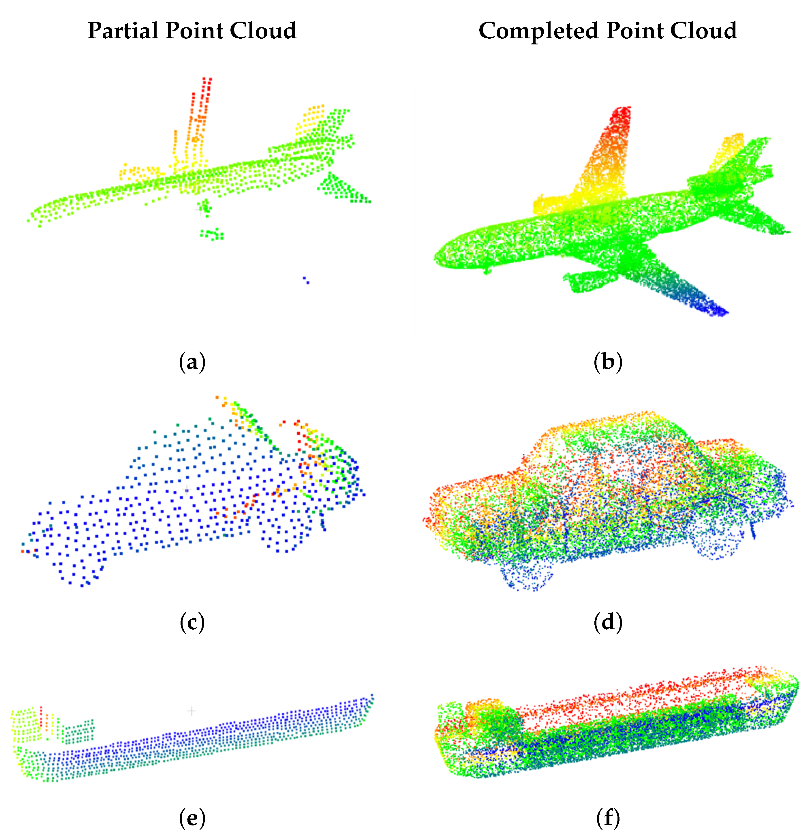
2.1. Point Cloud Completion Networks

Point cloud completion is essential in 3D understanding. As more and more real-world applications are tackled, there need to be innovative methods of handling occlusions and viewpoint challenges [11]. This section discusses deep learning point completion methods [12,13].

Point Completion Network [14] (PCN) was one of the first proposed techniques. PCN presents an autoencoder that takes a partial point cloud as input and returns a complete point cloud. More recent methods incorporate folding techniques to enforce better spatial resolution. Point Fractal Net [15] incorporates hierarchical elements extracting point features with different downsampling layers. Finally, methods such as TopNet [16] propose a hierarchical tree structure to present fine-grain details. Current point completion methods mainly focus on the Completion3D [2,14,16], and Point Cloud Completion Network [14] datasets which consist of synthetic point clouds constructed from the ShapeNet dataset.

2.1.1. PointNet Features

A commonality amongst all point cloud completion methods is their use of PointNet features in the encoder. PointNet is the most common of the pointwise MLP methods and stands out as one of the first architectures to take raw points without any intermediate representation [6,8,17,18]. PointNet is a versatile architecture with three major applications; classification, part segmentation, and semantic segmentation [19,20,21]. This work will focus on PointNet vanilla, which refers to the specific combination of operators that transforms the raw point cloud into a single global feature descriptor.

2.1.2. Folding-Based Decoders

Most of the methods covered use standard PointNet features for the encoding layer. This section will describe the recent progress in the decoding layers, specifically introducing a folding operation for point cloud reconstruction.

Initial research in point cloud decoders used a series of fully connected layers to transform the codewords learned in the latent space. These fully connected layers have many parameters, limiting the size of the point clouds which are reconstructed. Additionally, the fully connected layers could reconstruct general shapes but struggle to convey local geometric regions. FoldingNet introduces a unique folding operation that takes a 2D grid as input and deforms it around a 3D shape. The authors suggest introducing a 2D grid and then performing deformable operations, such as cutting, squeezing, and stretching, to match the 3D surface. This 2D grid mimics the implicit surface which is described by the 3D points.

The folding operation begins at the latent space. A 2D grid, the same size as the number of desired points, is initiated and is concatenated with the replicated codewords from the latent space. A folding operation can produce any arbitrary point cloud shape with a minimum two-layer perceptron. The final decoder is a concatenation of two folding operations. Compared to a fully connected layer, the total decoder has around 7% of the total parameters. Folding-based decoders are among the most popular decoders for point cloud completion networks.

2.1.3. Skip Attention Network

Skip Attention-Net (SA-Net) acknowledges information loss in the local regions of the incomplete point cloud, which is present in most point cloud completion methods. A skip attention module is suggested to use the fine details from partial point clouds. Passing local geometric information via the skip attention module can recreate the entire geometry at several scales. A decoder that uses hierarchical folding is also proposed to preserve the structure.

Like many others, SA-Net uses PointNet++ [22,23] as their backbone feature extractor and encoder. PointNet++ uses a hierarchical structure, features are extracted at multiple sampling levels, with the last level representing the global cloud feature. Once the point features are calculated, the features pass to the decoder. After going through the skip attention module, each hierarchical feature set passes to a different decoder level. A folding block increases the number of available features.

The folding block contains two elements: the up module and the down module. The up module replicates the features to the desired sampling rate, and the features are combined with 2D occupancy grids. The 2D grids are passed through MLPs to increase the dimensionality to 3D. These 3D features are considered codewords. This process continues, concatenating each hierarchical layer with the previous one. MLPs construct a self-attention module that highlights associations between features. Finally, the output of this self-attention module flows to the down module.

The down module is a spatial refinement where the expanded point features aggregate to one local point feature. This aggregation is followed by an MLP and another instance of the up module. The skip attention module provides the bridge between the local features extracted in the encoder and the features expected by the decoder. Adding the skip attention module to the traditional encoder–decoder structure fuses features of the same region and propagates the parts of similar geometric areas. Most objects contain some degree of symmetry, and often interlocal geometries can be used from other portions of the imagery. The skip-attention module in SA-Net calculates the pattern similarity, using cosine similarity, between local regions of the incomplete point cloud and local areas of the completed points cloud. Similar regions are selectively fused using the attention-weighted sum.

SA-Net successfully outperforms other shape completion methods in both the Completion 3D network and the KITTI [24] dataset. This result is also significant because the KITTI dataset comprises real-world lidar information instead of the typical synthetic point clouds.

2.2. Sampling Methods

Downsampling is a standard operation in 3D point clouds [18,25]. Typically, there are two places where one might like to downsample. The first is downsampling a point cloud before inputting it into the network. Deep learning networks for point clouds usually take a set number of points as the input; the problem of context versus resolution is critical.

Clipping the scenes into smaller chunks may make the point cloud more manageable, but if it is a very dense point cloud, the clipped areas may not provide enough contextual information for tasks such as semantic segmentation. A standard solution is downsampling a point cloud before inputting it into the network to keep enough context and control the number of input points.

Another area where downsampling occurs is hierarchical downsampling within the network. For example, tasks that rely on per-point results, such as point cloud generation or semantic and instance segmentation, rely on a hierarchical encoder [26,27,28,29,30,31]. This configuration extracts features from different levels created by downsampling the point clouds with different ratios. For example, a network might extract local point features from the input points and then downsample these points and extract local point features again from the downsampled points. This hierarchical approach allows the network to examine the cloud at different levels of detail and extract more information to form global features. This sampling work will focus on solutions for hierarchical sampling.

2.2.1. Farthest Point Sampling

The most commonly used hierarchical sampling technique is farthest point sampling (FPS) [32,33,34,35]. In this method, the first point is chosen arbitrarily. The next point chosen is the farthest point from the initially selected point. Points are chosen continuously, each time selecting the new point to be the point that is as far away as possible from the set of previously selected points. This method is robust to differences in resolution within the scene. For example, one area may have a dense resolution, while another area has a sparse resolution. When randomly sampling, it is common to miss key points in the sparsely populated area; however, FPS mitigates this issue by getting spatially diverse points.

2.2.2. SampleNet

Learned sampling is relatively new, with several recently proposed methods [36,37]. The most famous example is SampleNet. SampleNet [38] aims to reduce the computational demands of point cloud processing by introducing a learned sampling. The output of most sensors produces a large number of points, in some cases, millions of points per scene. However, most point cloud networks can take only small batches containing several thousand points, so sampling is standard. Traditional sampling methods, such as random sampling or FPS, do not consider the overall task. SampleNet proposes learning the selection at the same time as the task. The network can choose points tailored to that specific task by learning simultaneously. A uniquely tailored sampling can be developed for classification, registration, and reconstruction tasks. This method also addresses the issue of differentiability in point clouds and proposes a method to solve this [39]. SampleNet has three primary outputs—simplified points, sampling points, and projected points. The simplification takes the original point cloud as an input and processes them using an MLP. The output features of the MLP are then max-pooled. Finally, the max-pooling operation results are run through a fully connected layer that gives the simplified points.

Using the simplified points directly, as in FPS, is not ideal because point matching is not differentiable. This lack of differentiability means that the task loss is not propagated back to the sampling network. To tackle this issue, SampleNet also proposes a soft-projection network. The soft projection operation takes the original input point cloud and the simplified points. Then, each simplified point is transformed onto a local space, where a weighted average of its nearest neighbors determines the projected point’s location.

The final result of this process is a projected point set. A point cloud represents an underlying shape, so the projection better describes the underlying form rather than choosing any particular set of points within the original point clouds. Projected points are fed into the task during training. At evaluation time, the soft projection is replaced with the sampling; for each projected point, the network chooses the original point with the greatest weight. The evaluation enforces a unique set, replacing repeated points with points selected using an FPS.

2.3. Loss Functions

The following sections examine the effect of loss functions in 3D point cloud applications. In 2D data, the mean squared error and the binary cross-entropy are the primary reconstruction loss functions [40]. However, these cannot be used directly with 3D points because of permutation invariance. Both mean squared error and binary cross-entropy require a one-to-one correspondence between the prediction elements and the ground truth.

A matching function must be implemented to link corresponding points between the datasets. Once the points are matched between the two-point sets, the distance between the input and output points is the traditional loss. For a distance measure to be a useful loss function for point clouds, it must satisfy several conditions. It must be differentiable between point locations, it must have an efficient computation, and it must be robust against outliers. Using a 3D distance as a loss function is advantageous because it measures an actual distance instead of a “pixel” space. In a 2D image, without additional camera information, it is impossible to tell the exact distance between objects because it is so highly dependent on the viewpoint. For 3D point clouds, the distance can be calculated directly. This distance will provide an advantage when coming up with our encodings. In terms of distance metrics as direct loss functions, two main ones are explored: Chamfer distance, and Earth Mover’s distance [41].

2.3.1. Chamfer Distance

The first requirement of the Chamfer distance [42] is the nearest neighbor matching between point sets [43]. Nearest neighbor matching, also sometimes called greedy matching, is the most common matching algorithm [44,45,46]. The treated points and the control points are considered. The treated points are the points we are finding matches for, and the control points are the points we are matching to. Given some criteria, the closest point in the control set is found for each point in the treated set. In our case, this criteria will be Euclidean distance. This method is greedy because it does not consider whether the chosen control point has matched any other treated point. Multiple treated points can be matched to a single control point when performing a nearest neighbor matching. Similarly, it is also possible that some control points are not matched to any treated points. Unlike one-to-one matching, nearest neighbors matching is much more computationally efficient than other matching functions because of its lack of optimization criteria.

The computational efficiency makes it ideal for a deep learning application, but this method can struggle in point clouds with a high density of points in any part of the point cloud. Too many treated points matched to a single control point will cause undesirable results. CD is calculated between two point clouds by first calculating nearest neighbors from cloud $S_1$ to cloud $S_2$ and then taking the sum of the minimum squared distance from each point. This process is repeated with the nearest neighbors from cloud $S_2$ to cloud $S_1$. The summation of these two calculations becomes the final distance measure. The CD equation between two point clouds, $S_1$ and $S_2$, is shown below:

$$D_{CD}(S_1,S_2)=\sum _{x\in S_1}{min}_{x\in S_2}\left|\right|x-x^{\prime }{\left|\right|}_2^2+\sum _{x^{\prime }\in S_2}{min}_{x\in S_1}\left|\right|x-x^{\prime }{\left|\right|}_2^2$$

(1)

As a distance measure, this has many advantages, primarily its computational efficiency. The distance search for each point is independent, so the nearest neighbors search is parallelizable. Additionally, structures such as KD trees can be utilized for more efficient computation. Although the CD has many advantages, it is not bijective. As a result, the nearest neighbors’ search does not require a one-to-one point correspondence between the matches, allowing for point clustering in unevenly distributed point clouds.

2.3.2. Earth Mover’s Distance

Earth Mover’s Distance (EMD), sometimes called the Wasserstein distance, is the last point cloud distance function [47]. The goal is to do the least amount of work to move one model to match the other. Mathematically, this process takes one distribution and moves elements to match the distribution to a target distribution. For two sets of point clouds, a one-to-one matching is assigned from a point in one group to a point in the other. Each potential match has an associated cost, the distance between the two matched points. The goal is to match each point from set $S_1$ to a different point in $S_2$ while minimizing the total cost. The process is a linear assignment problem, where each point is a cluster whose weight is equal to that of all the other points.

This equation implies bijection. Each point in the reference set is matched to one unique point in the target set and vice versa. The optimal bijection is unique and invariant for all point locations.

Unfortunately, this calculation is expensive and impractical for a loss function. An approximate EMD is shown in Equation (2), where $\varphi$ represents the best matches found in a set number of iterations [48]. In experiments, the approximation error is relatively low, less than 1%, as shown in [41]. Although this approximation speeds up the EMD calculation considerably, it is still much slower than the CD.

$$D_{EMD}(S_1,S_2)=mi{n}_{\varphi :S_1\to S_2}\sum _{x\in S_1}\left|\right|x-\varphi \left(x\right){\left|\right|}_2$$

(2)

This section outlines the current state-of-the-art point cloud completion and processing techniques. Although there has been considerable advancement in this area over the last few years, there is still more work to be done. The next sections will focus on proposed improvements to the hierarchical sampling and point distance loss functions.

3. Materials and Methods

The main objective of this research was to implement and evaluate our proposed method to reduce occlusions in point clouds. This section will review the two datasets used for evaluation, DALES Viewpoints Version 2 and the PCN dataset. We will also outline our proposed method, specifically, a new point cloud sampling technique which allows for feature-based sampling and a parallel network structure that generalizes the feature learning for multiple augmentations and viewpoints.

3.1. Point Cloud Network Dataset

The first dataset is the Point Cloud Completion Network(PCN) dataset [14]. This dataset is derived from ShapeNet [2], which provides over 50 thousand unique models with over 55 categories, including all 12 Pascal 3D+ types. The key features of this dataset are the clean models and the consistent orientation.

This work follows PCN in the dataset creation to refine ShapeNet Core for the 3D completion task. First, 30,974 objects are chosen from eight categories: airplane, cabinet, car, chair, lamp, sofa, table, and vessel. Each mesh surface is sampled uniformly, using 16,384 total points. 2D depth images are backpropagated into 3D to form partial inputs for each model. These backpropagations aim to simulate a view occlusion that would occur in an actual sensor. Eight random viewpoints are chosen per cloud, resulting in eight separate partial clouds for each object. The validation set contains 100 objects, and the testing set contains 150 objects. The data will be two point cloud pairs; the first is a partial cloud created from the 2D depth mapping, and the second is a fully sampled cloud created from the original ShapeNet mesh object. Some examples of partial point clouds from the PCN dataset are in Figure 1.

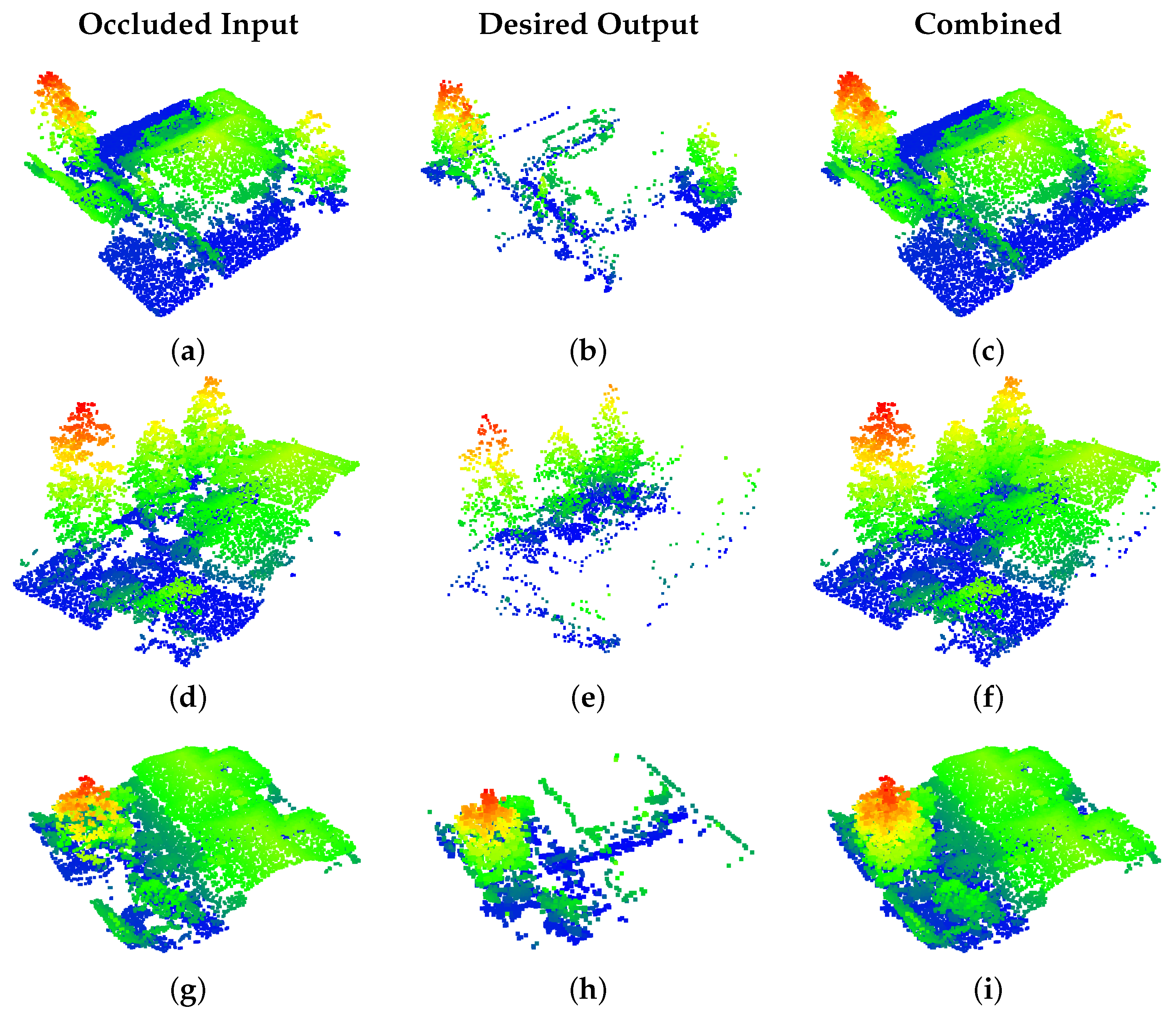
3.2. DALES Viewpoints Version 2 Dataset

Previous occlusion reduction work produced the DALES Viewpoints Version 1 dataset [49]. This dataset consists of 2048 input points with occluded areas and 2048 output points representing the point cloud without occlusions. Although this dataset was initially helpful, we recreated these data to address several critical issues in the initial version. These fundamental issues include the low resolution per scene and the reproduction of points between the input and output point clouds. We call this new dataset DALES Viewpoints Version 2.

The first issue was the low resolution of the DALES Viewpoints Version 1. In response to the low-resolution issue, the resolution of the input points was increased from 2048 to 16,384. The number of output points is the same, 2048. These additional points will help to improve the visual quality of the results and allow us to have the resolution necessary to perform more complex post-processing tasks such as registration and semantic segmentation.

Next, the number of occluded points and the number of viewpoints are addressed. The off-nadir angle is increased to create the additional occluded areas, moving from 26 degrees to 30 degrees. This extra movement off-nadir will increase the occluded regions to be about 20–25% of the whole scene. This increase in occluded areas will present a more challenging task to the network. The number of available viewpoints also increases, moving from one per scene to four per scene. This setup simulates a platform moving from each corner of the scene, allowing multiple occlusion scenarios per scene. Figure 2 shows a single DALES Viewpoints Version 2 scene simulated from four distinct flying patterns.

Finally, the DALES Viewpoints Version 2 reframes the occlusion reduction problem as a point inpainting problem. Instead of accepting input points and then regenerating the entire scene, both the input points and the occluded area, the network is tasked with generating only the occluded region. The whole scene is constructed by combining the input and output points. This restructuring has two advantages; the first is that it allows the network to generate a higher-resolution scene while also reducing the parameters needed; instead of rendering 16,384 points, only 2048 need to be generated. Additionally, the overall scene is still a higher resolution of 18,882 points. This reconstruction also gives the network a more challenging task: instead of recreating points, the network must generate a set of totally new points. Image examples of several point cloud scenes from the new DALES Viewpoints Version 2 dataset are in Figure 3. Each scene chip has a greater total area, displaying a complete scene. Each chip also has a higher resolution and more occluded areas than the DALES Viewpoints Version 1 dataset.

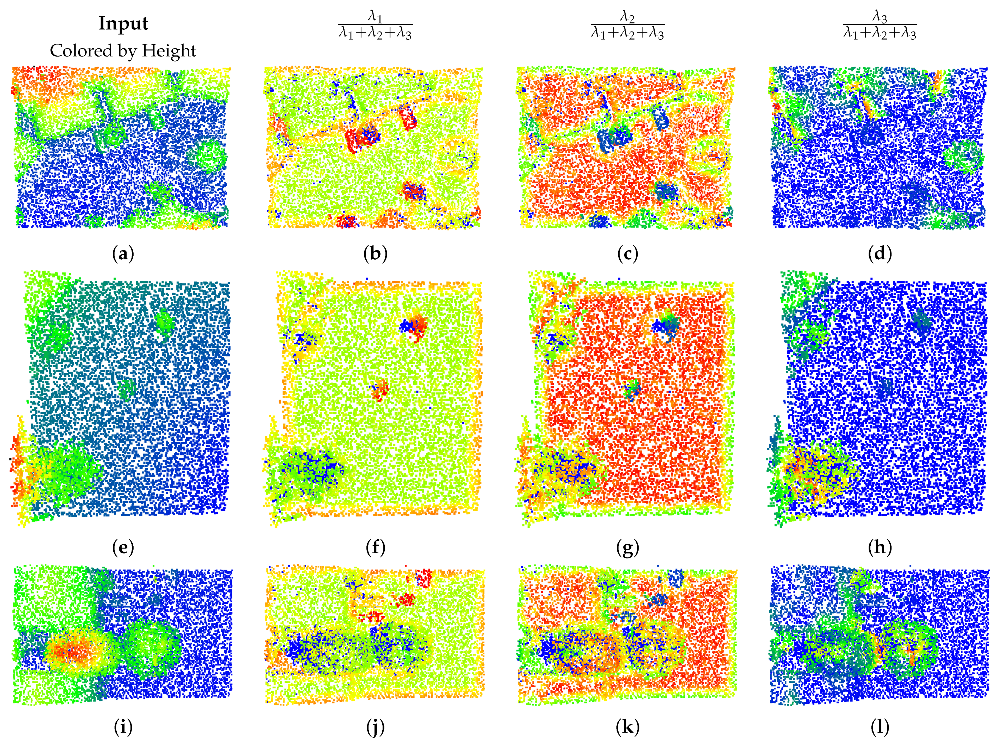
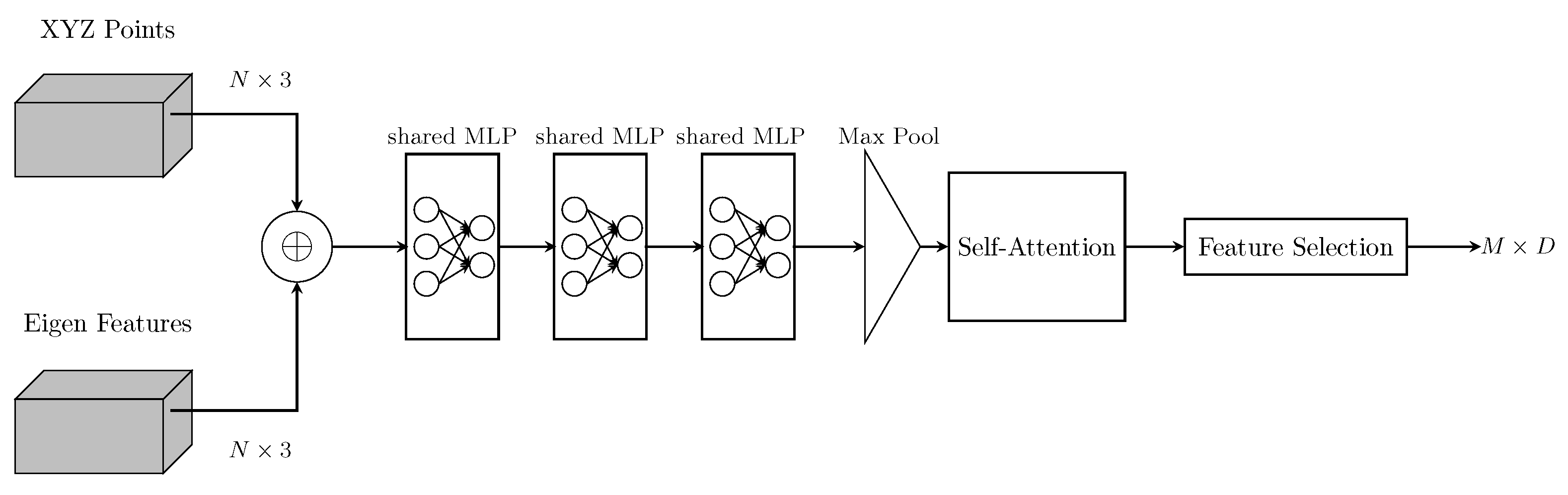
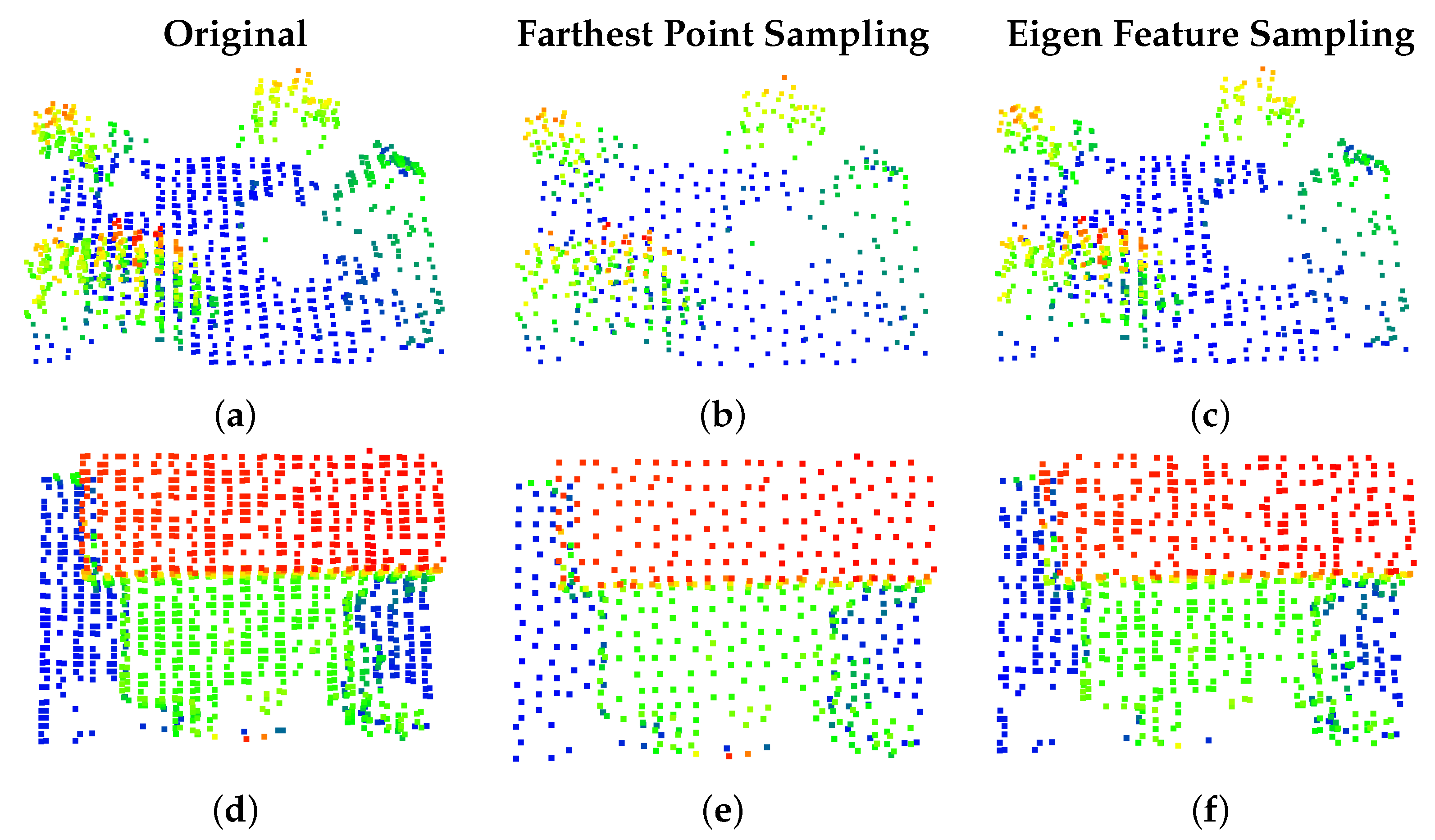
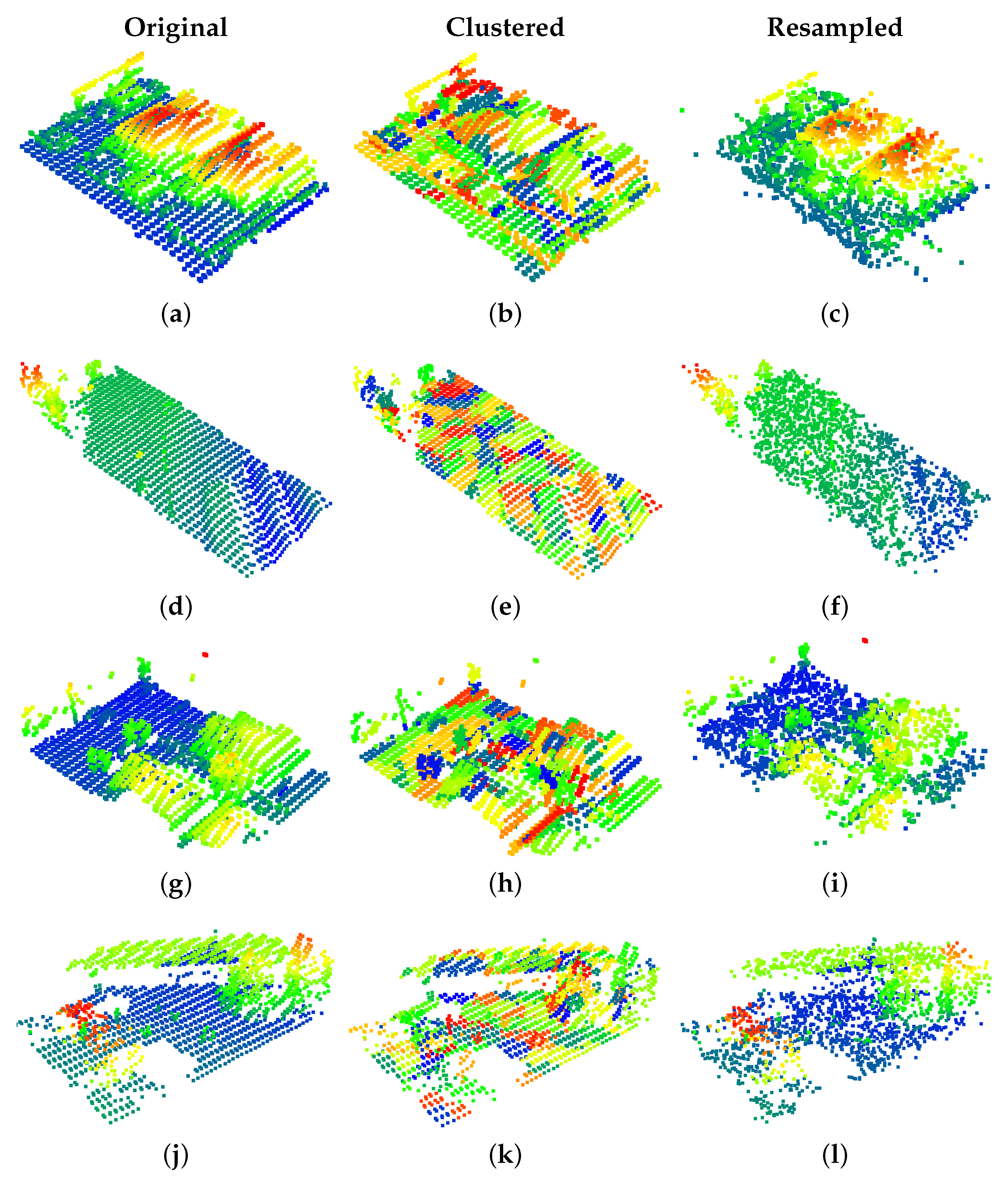
3.3. Eigen-Based Heiarchical Sampling

Our first objective for this proposal is to design a task-specific hierarchical sampling for our encoder. In point cloud generation algorithms, most encoders have a hierarchical structure in which we calculate local point features for downsampled versions of the point clouds. This hierarchical downsampling approach is very prevalent in the deep learning and image processing fields, with U-Net [50] being one of the most famous examples. PointNet++ popularized this idea in point clouds, using FPS.

We propose a different approach to learned sampling designed to select points based on anticipated areas of focus. Although the context of the entire scene is essential, we will only need to generate occluded points in some areas of the scene. We do not necessarily want an even sampling, but instead, we want to adjust our sampling ratios to sample heavily in detail areas and have a less frequent selection in areas with low detail. We define this as areas with a high frequency of change in one or more directions, which can be expressed using local eigenvalues. Figure 4 shows an example of how local eigenvalues can express important information about the scene contents.

First, we perform a radius search on the points to establish local point neighborhoods. P represents the entire point cloud of dimension $N\times 3$ and $P_s$ corresponds to each point in the cloud, where s ranges from 1 to N. $P_k$ represents one of the points in the set of K nearest neighbors of $P_s$. We calculate a covariance matrix ${\Sigma }_s$ using the following equation, where ${\mu }_s$ denotes the mean of the K nearest neighbors of $P_s$.

$${\Sigma }_s=\sum _{k=1}^K{(P_k-{\mu }_s)}^T·(P_k-{\mu }_s)$$

(3)

${\Sigma }_s$ is a $3\times 3$ matrix whose eigenvalues are defined as the roots of the following equation:

$$det({\Sigma }_s-{\lambda }_{s}I)=|{\Sigma }_s-{\lambda }_{s}I|=0$$

(4)

We extract the eigenvalues and concatenate them with our point set to form our initial features of size $N\times 6$. The first three dimensions are the X, Y, and Z, and the final three are the eigenvalues of size $N\times 3$ for each point. We then run this set of features through a series of shared multilayer perceptrons of size $64\to 128\to 256\to 512$, with the final output layer being the same size as the number of points that we wish to downsample to, in this case, size M. The output of the shared multilayer perceptrons are local features for each point, of size $N\times M$. We then integrate a self-attention module that helps establish relationships between each point feature. For each point $P_s$, we want to establish an attention score, $a_{s,j}$ for $j=1,2,\cdots ,N$.

First, the attention scores are calculated using the following equation:

$$a_{s,j}=\frac{exp(MLP{\left(P_s\right|{\beta }_h)}^T·MLP\left(P_j\right|{\beta }_l))}{{\sum }_{n=1}^{N}exp(MLP{\left(P_s\right|{\beta }_h)}^T·MLP\left(P_n\right|{\beta }_l))}$$

(5)

$MLP$ represents a multilayer perceptron with distinct input and output parameters. We defined ${\beta }_h$ and ${\beta }_l$ to have input layers equal to the downsampling and output layer of size 64. The calculation of the attention score is equivalent to a matrix multiplication between $MLP{\left(P_s\right|{\beta }_h)}^T$ and $MLP\left(P_j\right|{\beta }_g)$ followed by a soft-max operation. Once we obtain the values for $a_{s,j}$, we run the original input through another multilayer perceptron $MLP\left(P_j\right|{\beta }_h)$ to obtain our final attention matrix. This attention matrix is then added to the original inputs to form our final output. This final step is below.

$$P_s⟵P_s+\sum _{j=1}^N{a}_{s,j}·MLP\left(P_j\right|{\beta }_g)$$

(6)

After the self-attention is applied, we still have features of size $N\times M$. Our final desired output is a feature of size $M\times 3$. We then calculate the variance of each point feature and remove points that have low variance features. Finally, we perform a max-pooling operation on the set of attributes and take the top M unique points contributing to the feature set. The final output is the index of points in set $N\times 3$, which we will use to select our downsampled set of size $M\times 3$. The entire sampling architecture is shown in Figure 5 and the feature selection method is in Figure 6. Finally, we can observe our Eigen feature sampling when compared against the FPS in Figure 7. We see that there are distinct differences between our sampling and the FPS. The FPS is evenly sampled, where our Eigen feature sampling is denser in some areas than others. The edges in the Eigen sampling, especially those around the occluded areas, have much more points than in the FPS scenes.

3.4. Point Correspondence Loss

This section presents a method to address the shortcomings of loss functions that require point-to-point correspondence. Existing strategies have focused on developing a secondary representation to address the underlying structure. We will take a different approach and guide the features into a standard representation for any points set depicting the same scene.

The first step is to develop a method that suggests alternative point correspondences given an input point cloud. For example, one common way to do this is point jittering. Point jittering is a standard data augmentation method where random Gaussian noise is added to the point cloud to make an alternative representation. As a method of augmentation, this allows a slight improvement in the overall performance. However, random Gaussian noise in any direction causes a blurring of the scene and places points in new locations that may or may not represent the underlying structure. Therefore, we propose a new method to suggest alternative point correspondences using a Gaussian mixture model to split the scene into a set number of components and resample based on the characteristics of the individual components.

The Gaussian function is a widely used descriptor, having only two parameters for a normalized Gaussian: the mean and the standard deviation. This lack of parameters limits our ability to describe complex data.

Suppose the data we wish to model is too complex to be expressed as a single Gaussian distribution. In that case, we consider this data as multimodal, having several different areas or components with high probability. Thus, we express our model as a mixture of elements where each element is in a single parametric form: the Gaussian. We define a Gaussian mixture as $i\in \{1,\dots ,L\}$, where L represents the number of components, which is given explicitly. Each Gaussian has the following parameters, ${\mu }_i$ that defines the mean, ${\Sigma }_i$ which expresses the covariance and ${\varphi }_i$ which is a mixing coefficient which fulfills the following equation:

$$\sum _{i=1}^L{\varphi }_i=1$$

(7)

The Gaussian function, $\mathcal{N}$, is defined below, where P describes our three-dimensional data points.

$$\mathcal{N}\left(P\mid {\mu }_i,{\Sigma }_i\right)=\frac{1}{\sqrt{{\left(2\pi \right)}^L\left|{\Sigma }_i\right|}}exp\left(-\frac{1}{2}{\left(P-{\mu }_i\right)}^{\mathrm{T}}{\Sigma }_i^{-1}\left(P-{\mu }_i\right)\right)$$

(8)

We define the probability of any given data point in the equation below.

$$Prob\left(P_s\right)=\sum _{i=1}^L{\varphi }_i\mathcal{N}\left(P_s\mid {\mu }_i,{\Sigma }_i\right)$$

(9)

Next, we use Expectation Maximization (EM) to solve for the component assignments, $C_i$ for each datapoint $P_s\in P$ for the model parameters ${\varphi }_i,{\mu }_i,\mathrm{and}{\sigma }_i$. We perform the expectation by calculating the components for each data point given the current model parameters.

$${\gamma }_{s,i}=Prob\left(C_i\mid P_s,\varphi ,\mu ,\sigma \right)=\frac{{\varphi }_i\mathcal{N}\left(P_s\mid {\mu }_i,{\sigma }_i\right)}{{\sum }_{j=1}^L{\varphi }_j\mathcal{N}\left(P_s\mid {\mu }_j,{\sigma }_j\right)}$$

(10)

According the the calculated ${\gamma }_{s,i}$, we update ${\varphi }_i$, ${\mu }_i$ and ${\sigma }_i^2$

$${\varphi }_i=\sum _{s=1}^N\frac{{\gamma }_{s,i}}{N}$$

(11)

$${\mu }_i=\frac{{\sum }_{s=1}^N{\gamma }_{s,i}{P}_s}{{\sum }_{s=1}^N{\gamma }_{s,i}}$$

(12)

$${\sigma }_i^2=\frac{{\sum }_{s=1}^N{\gamma }_{s,i}{\left(P_s-{\mu }_i\right)}^2}{{\sum }_{s=1}^N{\gamma }_{s,i}}$$

(13)

The updates continue until the parameters ${\theta }_t$ at iteration t are below a predetermined threshold, $ϵ$.

$$\left|{\theta }_t-{\theta }_{t-1}\right|\le ϵ$$

(14)

We can perform clustering directly by using the Bayes Theorem to calculate the probability of any data points $P_s$ belonging to component $C_i$.

$$Prob\left(C_i\mid P_s\right)=\frac{Prob\left(P_s,C_i\right)}{Prob\left(P_s\right)}=\frac{Prob\left(C_i\right)Prob\left(P_s\mid C_i\right)}{{\sum }_{j=1}^{K}Prob\left(C_j\right)Prob\left(P_s\mid C_j\right)}=\frac{{\varphi }_i\mathcal{N}\left(P_s\mid {\mu }_i,{\sigma }_i\right)}{{\sum }_{j=1}^L{\varphi }_j\mathcal{N}\left(P_s\mid {\mu }_j,{\sigma }_j\right)}$$

(15)

We can sample new points according to the given component parameters. We show examples of the input points, clusters, and resampled data in Figure 8.

3.5. Parallel Network

For each input point cloud, we generate one alternative point correspondence cloud. We then run both the input and the alternative point cloud through the network. We wish to compare the latent spaces between the input and the alternative point cloud and guide the feature set to create the same latent space features for both these point clouds. To enforce this, we use a Mean Squared Error (MSE) loss to compare the latent spaces between the processed input point clouds and the processed alternate point clouds. Equation (16) expresses the MSE, where B represents the latent space vector from the original input point cloud, and $\widehat{B}$ represents the latent space vector from the noise added point cloud.

We wish to compare the features across each network feature layer, the three hierarchical layers of the encoder and the codewords. For the codewords, we can compare the features directly because we have a consistent representation of the features’ locations. However, the encoder layer features do not have a consistent order because of the permutation invariant nature of the point clouds. The shared MLP maintains this permutation invariance, but the MSE requires that we have element-to-element matching to compare the distance between the values. For this reason, we perform max-pooling on the encoder layers to transform them from local point features to a global feature.

$$L_{MSE}=\left|\right|B-\widehat{B}{\left|\right|}^2$$

(16)

The MSE loss will make up a portion of our overall loss function. To complete the loss function, we will also take a distance measure between the output of the decoder from the input point cloud and the output of the decoder from the alternative point cloud.

For distance metrics, we use both the EMD and the CD. Previous works [41] have noted that some metrics may perform better than others depending on the loss function. Therefore, we use CD for one output and EMD for the other when measuring the outputs. In this way, we can incorporate both metrics and improve our overall results. Equation (17) shows the total loss function, where EMD indicates the Earth Mover’s distance and CD indicates the Chamfer distance.

$$L_{\mathrm{total}}=EMD(P,GT)+CD(\widehat{P},GT)+MSE(B,\widehat{B})$$

(17)

The entire network diagram is shown in Figure 9.

4. Results

The final architecture is as follows: the general network architecture is an encoder–decoder construction. The encoder consists of PointNet++ features, replacing the initially proposed FPS with our Eigen Feature Selection Sampling. We want our Eigen Feature Selection radius to be large enough to provide local context, but small enough that our sampling remains efficient. After experimentation, we chose our radius for the Eigen calculation to be $\frac{1}{64}$th of the total scene size. The decoder is a folding-based architecture, using multiple discontinuous 2D grids as our initial folding shape. In addition, we employ skip-attention connection between each of the similarly sized layers between the encoder and decoder, respectively. This encoder-decoder represents the model. For training, we initialize two models and train in parallel, comparing the original input to its noisy output, averaging the weights after each training step.

Each network is trained with 400 epochs on a single NVIDIA Titan RTX. We use an Adam optimizer with an initial learning rate of 0.001. We maintain the reporting metrics for point cloud completion networks and use the mean CD, from Equation (1), similar to the Point Cloud Completion Network(PCN) results. We also report the mean EMD, from Equation (2), as an additional metric. We also comment on qualitative results, focusing on the visual completeness and overall realism of the point clouds.

4.1. DALES Viewpoints Version 2

The initial proposal of this network was to improve the appearance and subsequent post-processing of single-shot aerial lidar. We tested the proposed network on the DALES Version 2 dataset to assess this specific application. The performance is evaluated qualitatively by looking at the realism, general visual reconstruction and by examining the mean point distances between the predicted point cloud and the ground truth.

Figure 10 shows the overall results of our proposed network on the DALES Viewpoints Version 2 dataset. We see the original point cloud with occlusions, which is the input to our network, and the generated points combined with the original point cloud to make a fuller, richer point cloud with less occluded areas. We note that some of the most significant occluded areas are on the ground and around vegetation. Important points have been added in appropriate locations in these areas, and the occlusion is significantly reduced. We also see that our network is situationally aware. In Figure 10f, ground points are added appropriately under vegetation, where they would be expected, but the network refrains from adding additional points in unnecessary areas, such as beneath buildings. Finally, the algorithm is slightly noisy, with regions around structured objects, such as buildings or flat ground with some noise around the generated areas, which would not be present in a true unoccluded point cloud.

Figure 11 shows the reconstruction progression throughout the training. We can see that in the initial epochs, the network learns the occlusion locations, while later epochs make small changes and add detail levels.

We can observe how close the predicted and ground truth points match visually. Figure 12 shows examples of the input point clouds, as well as the generated and ground truth point clouds shown side by side. We observe a high degreeof fidelity between the predicted and the ground truth. The proposed network is successful in learning to mimic the expected shape and can predict multiple occluded areas, as seen in Figure 12b,k in separate parts of the scene. We note that the predicted point clouds have a slightly smoother contour and more jitter or random noise than the ground-truth clouds.

We can also observe the quantitative results shown in

Table 1. Overall results comparing our method to current state-of-the-art point cloud completion methods on the DALES Viewpoints Version 2 dataset.

Overall Results: DALES Viewpoints Version 2 Dataset
Method	Mean CD ↓	Mean EMD ↓
TopNet [16]	0.002167	0.071537
PCN [14]	0.001802	0.068283
ATLASNet [51]	0.000474	0.067515
PointNetFCAE [16]	0.000468	0.112022
SA-Net [52]	0.000433	0.039664
FoldingNet [53]	0.000424	0.097007
Ours	0.000375	0.035604

. We show that our method outperforms all other state-of-the-art techniques in both the Chamfer and EMD metrics. We implemented six other state-of-the-art networks, choosing from the top performers in the Completion3D and PCN dataset. We saw that our results had a significantly lower distances in both categories. We also observe that the parallel network setup and the combination of using both the EMD and Chamfer’s distance in our loss function allows for consistent performance across both metrics, unlike other networks.

4.2. Point Cloud Completion Network

We also compared the overall results on our network to published methods on the PCN dataset. Although point cloud completion on synthetic data is not our direct application, we wanted to test our network in an “apples-to-apples” comparison against other point cloud completion methods.

Figure 13 shows the performance of our network on the PCN dataset. In this configuration, there are 2048 input points and 16,384 output points. The network is tasked with rearranging the set number of points to describe the shape fully. Our network successfully produced a wide variety of shapes throughout all eight classes. We can see from Figure 13 that the network can even produce convincing results from a severely reduced shape, as in the case of the chair image in Figure 13j.

We also consider the results regarding the distance from the ground truth cloud.

Table 2. Point cloud completion comparison on Point Cloud Completion dataset in terms of per point Chamfer distance $\times {10}^4$ (lower is better).

Overall Results: Point Cloud Completion Network Dataset
Methods	Mean	Plane	Cab.	Car	Chair	Lamp	Couch	Table	Boat
AtlasNet [51]	17.69	10.37	23.4	13.41	24.16	20.24	20.82	17.52	11.62
FoldingNet [53]	16.48	11.18	20.15	13.25	21.48	18.19	19.09	17.8	10.69
PCN [14]	14.72	8.09	18.32	10.53	19.33	18.52	16.44	16.34	10.21
TopNet [16]	9.72	5.5	12.02	8.9	12.56	9.54	12.2	9.57	7.51
SA-Net [52]	7.74	2.18	9.11	5.56	8.94	9.98	7.83	9.94	7.23
Ours	7.10	2.51	10.29	10.29	8.07	6.54	6.64	6.61	5.87

shows the overall results; in this case, we only consider the Chamfer distance for consistency with other synthetic point cloud methods. Our network outperforms all others in the overall mean Chamfer distance and five out of the eight classes. Although we did not develop our method for this specific application, this shows that it could be used for a wide variety of applications and data types.

4.3. Discussion

4.3.1. Eigen Feature Selection Sampling

This section explores the effects of the proposed sampling method, compared to other common sampling techniques. For these experiments, we use the DALES Viewpoints Version 1 dataset. First, we examine the implementation using FPS sampling, then with the learned SampleNet, and finally, our Eigen Feature Sampling implementation. The quantitative results are in

Table 3. Comparison of the proposed sampling method against FPS and SampleNet learned sampling. Lower is better.

Ablation Study: Eigen Feature Sampling
Sampling Method	Mean CD ↓	Mean EMD ↓
FPS	0.00208	0.07594
SampleNet [38]	0.00282	0.13035
Eigen Feature Sampling (Ours)	0.00184	0.05244

.

We note that the original implementation with FPS has a mean Chamfer of 0.00208 and a mean EMD of 0.07595. The SampleNet learned sampling was less successful when compared to the initial FPS implementation. The mean Chamfer increased from 0.00208 to 0.00282, and the mean EMD increased from 0.07594 to 0.13035. We speculate two reasons for this worsened performance: the first is that this sampling method is exclusively tested with small CAD models. Secondly, we note that this sampling method is a pre-processing step for downsampling before the initial task. Thus, additional improvements may be needed to transform the SampleNet implementation for scene-based hierarchical sampling.

Finally, we implement our Eigen feature selection. We find that this gives an improvement over the FPS and SampleNet methods. We report a mean Chamfer of 0.00184 and a mean EMD of 0.05244. These results present an 11.6% improvement in mean Chamfer over the FPS method and a 31% improvement in mean EMD.

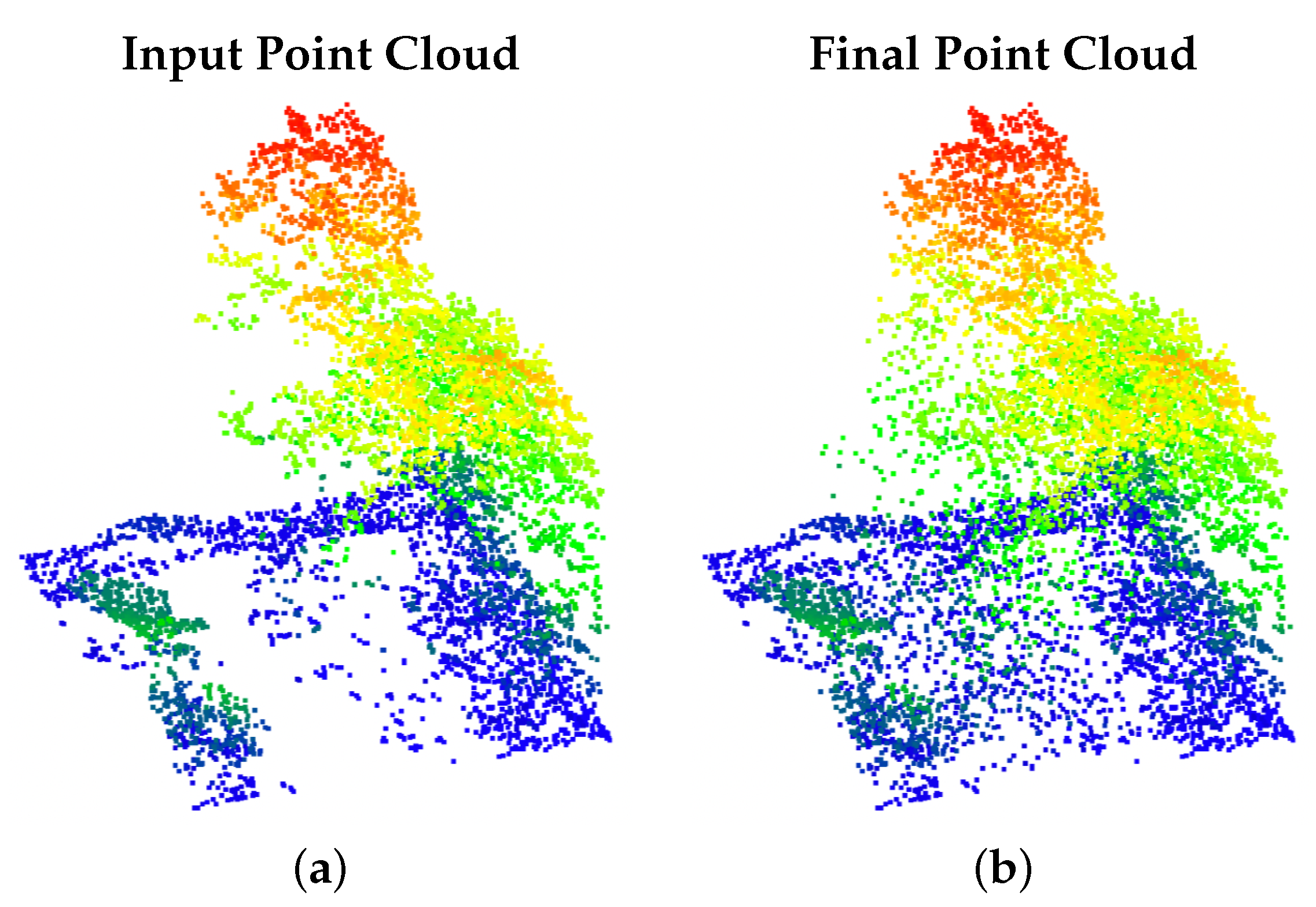
4.3.2. Point Projection for Stabilizing Point Correspondences

This next section examines the overall performance when comparing the single network implementation to our proposed Point Correspondence Loss with a parallel network setup. The overall performance results on the DALES Viewpoints Version 1 dataset are in

Table 4. Overall results on the DALES Viewpoints dataset comparing the original SA-Net implementation with the same implementation and our proposed point correspondence loss.

Ablation Study: Point Projection for Stabilizing Point Correspondences
Method	Mean CD ↓	Mean EMD ↓
Single Network	0.00208	0.07594
Parallel Network (Ours)	0.00167	0.04951

. We find that this setup significantly improves both metrics, with a 19.7% improvement in the mean Chamfer and a 34.8% improvement in the mean EMD from the single network implementation. Comparing feature channels between original and augmented feature levels allows a more robust network structure.

4.3.3. Timing

The parallel structure of our network has unique implications for the timing of our training. Each epoch consists of two runs of our network, one for the initial input and one for the augmented point cloud from the Gaussian mixture model. When comparing the timing for training between a single network and our parallel network, we find that we only need half as many epochs, with a single epoch representing two runs through our shared weight model.

We also see a slight timing improvement when comparing our Eigen Feature Selection Sampling and the FPS. The Eigen Feature Selection performs a single neighborhood operation at the initialization, while the FPS performs a neighborhood operation for each epoch. While this results in a significant improvement in the timing of the sampling module, the overall runtime is comparable with Skip Attention Net.

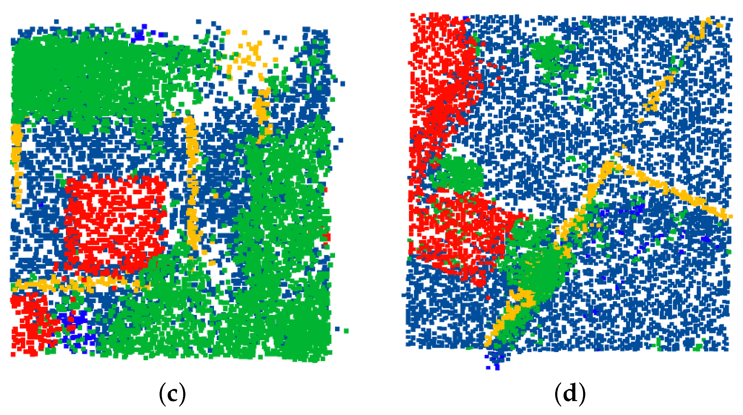
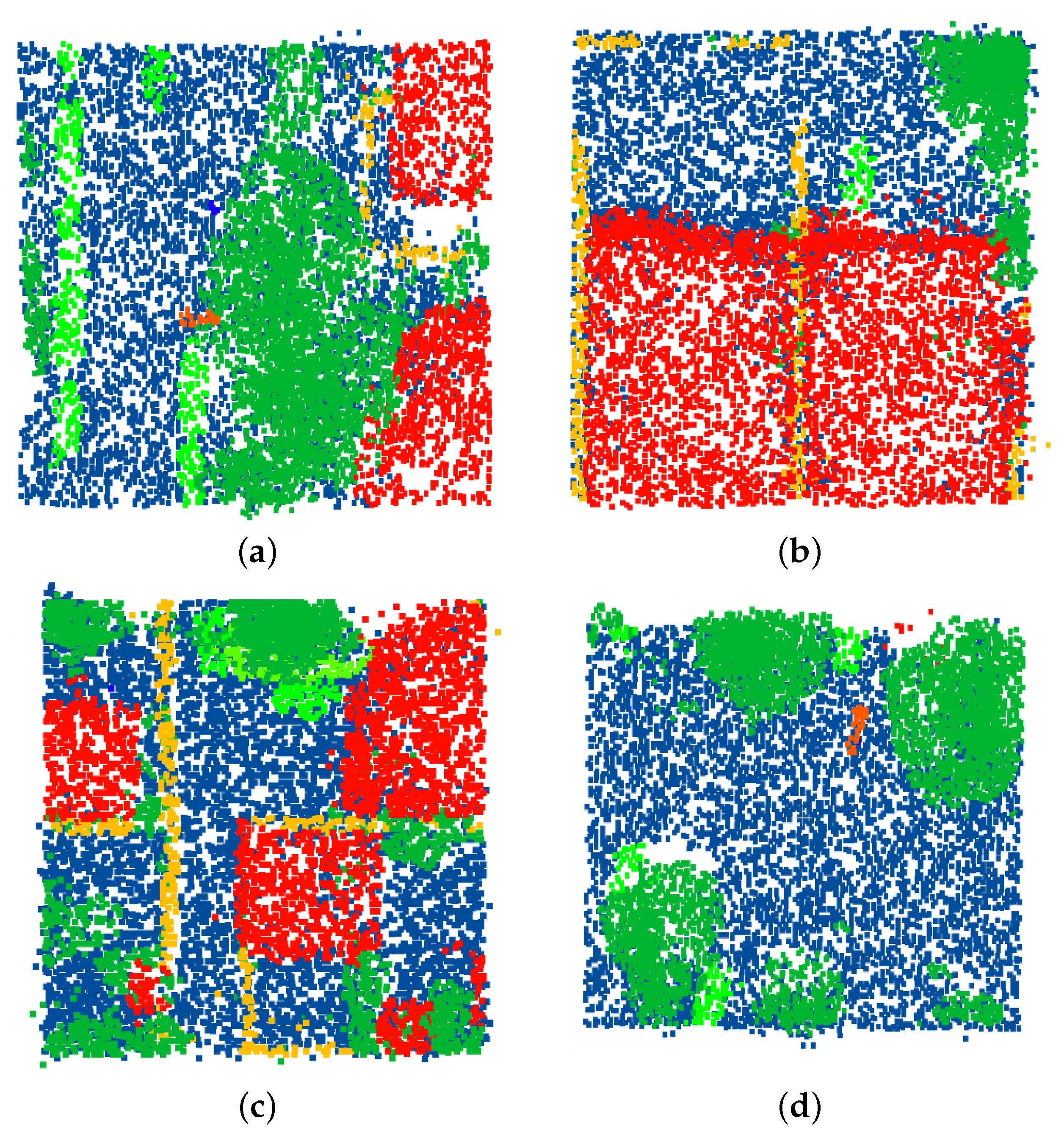
4.4. Semantic Segmentation

The final experiment that we run is the semantic segmentation experiment. Previous experiments have focused on comparing our generative network against other generative networks. This experiment focuses on the overall realism of our generated points and whether they can be successfully processed as part of a larger workflow.

Table 5. Comparison of the overall accuracy and mean IoU of the semantic segmentation results using the PointNet++ architecture. Dataset 1 refers to the DALES Viewpoints Version 2 dataset using only the input points containing occlusions. Dataset 2 refers to the DALES Viewpoints Version 2, which includes the input points with occlusions, supplemented by our generated points.

Semantic Segmentation: Overall Results
	Overall Accuracy	Mean IoU
Dataset 1	0.685	0.395
Dataset 2	0.865	0.451

shows the semantic segmentation’s overall results. We use the PointNet++ architecture to perform the semantic segmentation; the network is trained using the ground truth point clouds without occlusions. Dataset 1 refers to the semantic segmentation using only the point clouds with occlusions. Dataset 2 refers to the semantic segmentation using the point clouds with occlusions that have been supplemented with points generated by our occlusion reduction method. We can see that the overall accuracy of Dataset 2 is 18% higher, and the mean IoU increases by 5.5% when we generate the missing occluded points. We can see a significant increase in the semantic segmentation results when we generate a fuller point cloud that more closely matches the network’s data. These results also show that our generated points are realistic enough to be semantically segmented by a deep learning algorithm.

Table 6. Comparison of per class IoU, semantic segmentation results using the PointNet++ architecture. Dataset 1 refers to the DALES Viewpoints Version 2 dataset using only the input points containing occlusions. Dataset 2 refers to the DALES Viewpoint Version 2, which includes the input points with occlusions, supplemented by our generated points.

Semantic Segmentation: Per Class IoU
	ground	buildings	cars	trucks	poles	power lines	fences	veg
Dataset 1	0.740	0.713	0.266	0.262	0.204	0.660	0.148	0.556
Dataset 2	0.871	0.724	0.245	0.256	0.214	0.667	0.152	0.769

shows the per-class IoU. We can see that the semantic segmentation outperformed in six of the eight overall classes. The largest increase was in the vegetation and ground classes. This increase is expected because most occlusions happen in the ground vegetation and building classes, as these are the largest and most commonly occurring classes.

Examples of the visual results of the semantic segmentation are seen in Figure 14 and Figure 15. We can see that the overall semantic segmentation is successful. The reconstructed scenes are not overly noisy, and we can distinguish objects clearly. We see some confusion between the vegetation and car and truck class in Figure 15d, which is reflected in the per-class IoU results. Overall, the semantic labels successfully classified the vast majority of points. These results are a great indication that we can use our generated points as a pre-processing step to improve the performance in a wide variety of secondary tasks.

5. Conclusions

Data degradation and occlusions are considerable problems in point cloud processing. Recent research has focused on various applications, such as classification, semantic segmentation, instance segmentation, registration, and tracking. While research into these areas has made significant progress, most focus on heavily curated datasets. For example, ShapeNet and ModelNet present beautiful evenly sampled point cloud objects from synthetic CAD models. Even real-world datasets such as ScanNet and S3DIS present high-resolution, multi-scan data.

Collecting complete data may not always be an option in every scenario. Cost, time, and view angle limitations can result in point clouds with a significant number of occlusions. These occlusions make it difficult for human analysts to comprehend and can be difficult to process when most models are trained with complete, labeled datasets without occlusions.

This work frames occlusion reduction as a point cloud inpainting problem. We take successful algorithms in the point cloud completion space and add several key features to be successful in real-world occlusion reduction. We make two specific proposals: we propose a point cloud sampling method that can sample based on learned features within the point clouds instead of spatial resolution. We also offer a model structure and a point cloud loss configuration, which performs data augmentation to reduce the negative effects of different scanning patterns on the final reconstruction result.

We implemented these suggestions and showed that they significantly improved results when compared to current state-of-the-art point cloud completion networks. In addition to offering improved performance against other networks in traditional synthetic datasets, such as PCN, we also tested the method on two real-world datasets, using aerial LiDAR. This experiment is significant because it is the first quantifiable result for the point cloud completion problem on a real-world dataset. Previous experiments, for example, on the KITTI [24] dataset, only show a qualitative visual impact on real-world data, but no measurable results from the reconstruction.

We showed that our generated point clouds are closer to the ground truth when compared against other point cloud completion methods and are more visually appealing than their occluded counterparts. In addition to this, we demonstrated that these occlusion reduced point clouds, which could also be used as a pre-processing step in conjunction with other point cloud processing techniques. We trained a PointNet++ semantic segmentation network on the ground-truth point clouds from the DALES Viewpoint Version 2 data set. We then tested the semantic segmentation results on the point clouds with occlusions and the point clouds that had been filled in using our point clouds generation technique. We showed that point clouds enhanced using our method have an increased mean IOU compared to those that have not been enhanced with our methods.

References

1. Wu, Z.; Song, S.; Khosla, A.; Yu, F.; Zhang, L.; Tang, X.; Xiao, J. 3d shapenets: A deep representation for volumetric shapes. In Proceedings of the IEEE Conference on Computer Vision and Pattern Recognition, Boston, MA, USA, 7–12 June 2015; pp. 1912–1920. [Google Scholar]
2. Chang, A.X.; Funkhouser, T.; Guibas, L.; Hanrahan, P.; Huang, Q.; Li, Z.; Savarese, S.; Savva, M.; Song, S.; Su, H.; et al. Shapenet: An information-rich 3d model repository. arXiv 2015, arXiv:1512.03012. [Google Scholar]
3. Lemmens, M. Airborne lidar sensors. GIM Int. 2007, 21, 24–27. [Google Scholar]
4. Lehtola, V.V.; Kaartinen, H.; Nüchter, A.; Kaijaluoto, R.; Kukko, A.; Litkey, P.; Honkavaara, E.; Rosnell, T.; Vaaja, M.T.; Virtanen, J.P.; et al. Comparison of the selected state-of-the-art 3D indoor scanning and point cloud generation methods. Remote Sens. 2017, 9, 796. [Google Scholar] [CrossRef] [Green Version]
5. Carson, W.W.; Andersen, H.E.; Reutebuch, S.E.; McGaughey, R.J. LIDAR applications in forestry—An overview. In Proceedings of the ASPRS Annual Conference, Denver, CO, USA, 23–28 May 2004; pp. 1–9. [Google Scholar]
6. Li, Y.; Ma, L.; Zhong, Z.; Liu, F.; Chapman, M.A.; Cao, D.; Li, J. Deep learning for LiDAR point clouds in autonomous driving: A review. IEEE Trans. Neural Netw. Learn. Syst. 2021, 32, 3412–3432. [Google Scholar] [CrossRef] [PubMed]
7. Eitel, J.U.; Höfle, B.; Vierling, L.A.; Abellán, A.; Asner, G.P.; Deems, J.S.; Glennie, C.L.; Joerg, P.C.; LeWinter, A.L.; Magney, T.S.; et al. Beyond 3-D: The new spectrum of lidar applications for earth and ecological sciences. Remote Sens. Environ. 2016, 186, 372–392. [Google Scholar] [CrossRef] [Green Version]
8. Liu, W.; Sun, J.; Li, W.; Hu, T.; Wang, P. Deep learning on point clouds and its application: A survey. Sensors 2019, 19, 4188. [Google Scholar] [CrossRef] [Green Version]
9. Endo, Y.; Javanmardi, E.; Kamijo, S. Analysis of Occlusion Effects for Map-Based Self-Localization in Urban Areas. Sensors 2021, 21, 5196. [Google Scholar] [CrossRef]
10. Böhm, J. Facade detail from incomplete range data. In Proceedings of the ISPRS Congress, Beijing, China, 3–11 July 2008; Volume 1, p. 2. [Google Scholar]
11. Goyal, A.; Law, H.; Liu, B.; Newell, A.; Deng, J. Revisiting point cloud shape classification with a simple and effective baseline. In Proceedings of the International Conference on Machine Learning, PMLR, Online, 18–24 July 2021; pp. 3809–3820. [Google Scholar]
12. Chen, X.; Chen, B.; Mitra, N.J. Unpaired point cloud completion on real scans using adversarial training. arXiv 2019, arXiv:1904.00069. [Google Scholar]
13. Sarmad, M.; Lee, H.J.; Kim, Y.M. Rl-gan-net: A reinforcement learning agent controlled gan network for real-time point cloud shape completion. In Proceedings of the IEEE/CVF Conference on Computer Vision and Pattern Recognition, Long Beach, CA, USA, 15–20 June 2019; pp. 5898–5907. [Google Scholar]
14. Yuan, W.; Khot, T.; Held, D.; Mertz, C.; Hebert, M. Pcn: Point completion network. In Proceedings of the 2018 International Conference on 3D Vision (3DV), Verona, Italy, 5–8 September 2018; pp. 728–737. [Google Scholar]
15. Huang, Z.; Yu, Y.; Xu, J.; Ni, F.; Le, X. Pf-net: Point fractal network for 3d point cloud completion. In Proceedings of the IEEE/CVF Conference on Computer Vision and Pattern Recognition, Seattle, WA, USA, 13–19 June 2020; pp. 7662–7670. [Google Scholar]
16. Tchapmi, L.P.; Kosaraju, V.; Rezatofighi, H.; Reid, I.; Savarese, S. Topnet: Structural point cloud decoder. In Proceedings of the IEEE/CVF Conference on Computer Vision and Pattern Recognition, Long Beach, CA, USA, 15–20 June 2019; pp. 383–392. [Google Scholar]
17. Bello, S.A.; Yu, S.; Wang, C.; Adam, J.M.; Li, J. Deep learning on 3D point clouds. Remote Sens. 2020, 12, 1729. [Google Scholar] [CrossRef]
18. Guo, Y.; Wang, H.; Hu, Q.; Liu, H.; Liu, L.; Bennamoun, M. Deep learning for 3d point clouds: A survey. IEEE Trans. Pattern Anal. Mach. Intell. 2021, 43, 4338–4364. [Google Scholar] [CrossRef] [PubMed]
19. Aoki, Y.; Goforth, H.; Srivatsan, R.A.; Lucey, S. Pointnetlk: Robust & efficient point cloud registration using pointnet. In Proceedings of the IEEE/CVF Conference on Computer Vision and Pattern Recognition, Long Beach, CA, USA, 15–20 June 2019; pp. 7163–7172. [Google Scholar]
20. Sarode, V.; Li, X.; Goforth, H.; Aoki, Y.; Srivatsan, R.A.; Lucey, S.; Choset, H. Pcrnet: Point cloud registration network using pointnet encoding. arXiv 2019, arXiv:1908.07906. [Google Scholar]
21. Ge, L.; Cai, Y.; Weng, J.; Yuan, J. Hand pointnet: 3d hand pose estimation using point sets. In Proceedings of the IEEE Conference on Computer Vision and Pattern Recognition, Salt Lake City, UT, USA, 18–23 June 2018; pp. 8417–8426. [Google Scholar]
22. Qi, C.R.; Su, H.; Mo, K.; Guibas, L.J. Pointnet: Deep learning on point sets for 3d classification and segmentation. In Proceedings of the IEEE Conference on Computer Vision and Pattern Recognition, Honolulu, HI, USA, 21–26 July 2017; pp. 652–660. [Google Scholar]
23. Qi, C.R.; Yi, L.; Su, H.; Guibas, L.J. Pointnet++: Deep hierarchical feature learning on point sets in a metric space. arXiv 2017, arXiv:1706.02413. [Google Scholar]
24. Geiger, A.; Lenz, P.; Stiller, C.; Urtasun, R. Vision meets Robotics: The KITTI Dataset. Int. J. Robot. Res. 2013, 32, 1231–1237. [Google Scholar] [CrossRef] [Green Version]
25. Lu, H.; Shi, H. Deep Learning for 3D Point Cloud Understanding: A Survey. arXiv 2020, arXiv:2009.08920. [Google Scholar]
26. Thomas, H.; Qi, C.R.; Deschaud, J.E.; Marcotegui, B.; Goulette, F.; Guibas, L.J. Kpconv: Flexible and deformable convolution for point clouds. In Proceedings of the IEEE/CVF International Conference on Computer Vision, Seoul, Korea, 27 October–2 November 2019; pp. 6411–6420. [Google Scholar]
27. Hu, Q.; Yang, B.; Xie, L.; Rosa, S.; Guo, Y.; Wang, Z.; Trigoni, N.; Markham, A. Randla-net: Efficient semantic segmentation of large-scale point clouds. In Proceedings of the IEEE/CVF Conference on Computer Vision and Pattern Recognition, Seattle, WA, USA, 13–19 June 2020; pp. 11108–11117. [Google Scholar]
28. Wu, W.; Qi, Z.; Fuxin, L. Pointconv: Deep convolutional networks on 3d point clouds. In Proceedings of the IEEE/CVF Conference on Computer Vision and Pattern Recognition, Long Beach, CA, USA, 15–20 June 2019; pp. 9621–9630. [Google Scholar]
29. Maturana, D.; Scherer, S. Voxnet: A 3d convolutional neural network for real-time object recognition. In Proceedings of the 2015 IEEE/RSJ International Conference on Intelligent Robots and Systems (IROS), Hamburg, Germany, 28 September–2 October 2015; pp. 922–928. [Google Scholar]
30. Yang, B.; Wang, J.; Clark, R.; Hu, Q.; Wang, S.; Markham, A.; Trigoni, N. Learning object bounding boxes for 3d instance segmentation on point clouds. arXiv 2019, arXiv:1906.01140. [Google Scholar]
31. Makhzani, A.; Shlens, J.; Jaitly, N.; Goodfellow, I.; Frey, B. Adversarial autoencoders. arXiv 2015, arXiv:1511.05644. [Google Scholar]
32. Moenning, C.; Dodgson, N.A. A new point cloud simplification algorithm. In Proceedings of the 3rd IASTED International Conference on Visualization, Imaging, and Image Processing (VIIP 2003), Benalmadena, Spain, 8–10 September 2003; pp. 1027–1033. [Google Scholar]
33. Moenning, C.; Dodgson, N.A. Fast marching farthest point sampling for implicit surfaces and point clouds. Comput. Lab. Tech. Rep. 2003, 565, 1–12. [Google Scholar]
34. Landrieu, L.; Simonovsky, M. Large-scale point cloud semantic segmentation with superpoint graphs. In Proceedings of the IEEE Conference on Computer Vision and Pattern Recognition, Salt Lake City, UT, USA, 18–23 June 2018; pp. 4558–4567. [Google Scholar]
35. Yin, K.; Chen, Z.; Huang, H.; Cohen-Or, D.; Zhang, H. LOGAN: Unpaired shape transform in latent overcomplete space. ACM Trans. Graph. (TOG) 2019, 38, 1–13. [Google Scholar] [CrossRef] [Green Version]
36. Li, X.; Yu, L.; Fu, C.W.; Cohen-Or, D.; Heng, P.A. Unsupervised detection of distinctive regions on 3D shapes. ACM Trans. Graph. 2020, 39, 1–14. [Google Scholar] [CrossRef]
37. Yang, J.; Zhang, Q.; Ni, B.; Li, L.; Liu, J.; Zhou, M.; Tian, Q. Modeling point clouds with self-attention and gumbel subset sampling. In Proceedings of the IEEE/CVF Conference on Computer Vision and Pattern Recognition, Long Beach, CA, USA, 15–20 June 2019; pp. 3323–3332. [Google Scholar]
38. Lang, I.; Manor, A.; Avidan, S. Samplenet: Differentiable point cloud sampling. In Proceedings of the IEEE/CVF Conference on Computer Vision and Pattern Recognition, Seattle, WA, USA, 13–19 June 2020; pp. 7578–7588. [Google Scholar]
39. Dovrat, O.; Lang, I.; Avidan, S. Learning to sample. In Proceedings of the IEEE/CVF Conference on Computer Vision and Pattern Recognition, Long Beach, CA, USA, 15–20 June 2019; pp. 2760–2769. [Google Scholar]
40. Berger, J.O. Certain standard loss functions. In Statistical Decision Theory and Bayesian Analysis, 2nd ed.; Springer: New York, NY, USA, 1985; pp. 60–64. [Google Scholar]
41. Fan, H.; Su, H.; Guibas, L.J. A point set generation network for 3d object reconstruction from a single image. In Proceedings of the IEEE Conference on Computer Vision and Pattern Recognition, Honolulu, HI, USA, 21–26 July 2017; pp. 605–613. [Google Scholar]
42. Moore, A. The case for approximate Distance Transforms. In Proceedings of the The 14th Annual Colloquium of the Spatial Information Research Centre, University of Otago, Dunedin, New Zealand, 3–5 December 2002. [Google Scholar]
43. Fix, E.; Hodges, J.L., Jr. Discriminatory Analysis-Nonparametric Discrimination: Small Sample Performance; Technical Report; University of California: Berkeley, CA, USA, 1952. [Google Scholar]
44. Goldberger, J.; Hinton, G.E.; Roweis, S.; Salakhutdinov, R.R. Neighbourhood components analysis. Adv. Neural Inf. Process. Syst. 2004, 17. [Google Scholar]
45. Plötz, T.; Roth, S. Neural nearest neighbors networks. arXiv 2018, arXiv:1810.12575. [Google Scholar]
46. Wang, Y.; Sun, Y.; Liu, Z.; Sarma, S.E.; Bronstein, M.M.; Solomon, J.M. Dynamic graph cnn for learning on point clouds. ACM Trans. Graph. 2019, 38, 1–12. [Google Scholar] [CrossRef] [Green Version]
47. Levina, E.; Bickel, P. The earth mover’s distance is the mallows distance: Some insights from statistics. In Proceedings of the Proceedings Eighth IEEE International Conference on Computer Vision, ICCV 2001, Vancouver, BC, Canada, 7–14 July 2001; Volume 2, pp. 251–256. [Google Scholar]
48. Liu, M.; Sheng, L.; Yang, S.; Shao, J.; Hu, S.M. Morphing and Sampling Network for Dense Point Cloud Completion. arXiv 2019, arXiv:1912.00280. [Google Scholar] [CrossRef]
49. Singer, N.; Asari, V.K.; Aspiras, T.; Schierl, J.; Stokes, A.; Keaffaber, B.; Van Rynbach, A.; Decker, K.; Rabb, D. Attention Focused Generative Network for Reducing Self-Occlusions in Aerial LiDAR. In Proceedings of the 2021 IEEE Applied Imagery Pattern Recognition Workshop (AIPR), Washington, DC, USA, 12–14 October 2021; pp. 1–7. [Google Scholar]
50. Ronneberger, O.; Fischer, P.; Brox, T. U-net: Convolutional networks for biomedical image segmentation. In Proceedings of the International Conference on Medical Image Computing and Computer-Assisted Intervention, Munich, Germany, 5–9 October 2015; pp. 234–241. [Google Scholar]
51. Groueix, T.; Fisher, M.; Kim, V.G.; Russell, B.C.; Aubry, M. A papier-mâché approach to learning 3d surface generation. In Proceedings of the IEEE Conference on Computer Vision and Pattern Recognition, Salt Lake City, UT, USA, 18–23 June 2018; pp. 216–224. [Google Scholar]
52. Wen, X.; Li, T.; Han, Z.; Liu, Y.S. Point cloud completion by skip-attention network with hierarchical folding. In Proceedings of the IEEE/CVF Conference on Computer Vision and Pattern Recognition, Seattle, WA, USA, 13–19 June 2020; pp. 1939–1948. [Google Scholar]
53. Yang, Y.; Feng, C.; Shen, Y.; Tian, D. Foldingnet: Point cloud auto-encoder via deep grid deformation. In Proceedings of the IEEE Conference on Computer Vision and Pattern Recognition, Salt Lake City, UT, USA, 18–23 June 2018; pp. 206–215. [Google Scholar]
Figure 1. Examples of point clouds from the PCN dataset colored by height. The incomplete point cloud inputs are shown on the left, and the corresponding completed point clouds are shown on the right. (a) N = 2048, (b) N = 16384, (c) N = 2048, (d) N = 16384, (e) N = 2048, (f) N = 16384.
Remotesensing 14 02955 g001
Figure 2. A single scene from DALES Viewpoints Version 2, colored by height, with occlusions from multiple flight patterns. (a) Northwest to Southwest, (b) Southwest to Southeast, (c) Southeast to Northwest, (d) Northeast to Northwest.
Remotesensing 14 02955 g002
Figure 3. Examples of corresponding scenes from the DALES Viewpoints 2 data set, colored by height. The occluded input is in the left-hand column, the desired output is in the middle, and the combined full point cloud is on the right.
Remotesensing 14 02955 g003
Figure 4. Visual example local eigenvalues representing different spatial properties on the DALES Viewpoints Version 2 dataset. The original input point cloud is colored by height. The Eigen feature representations are colored by value, with warm tones indicating high values and cool tones indicating low values.
Remotesensing 14 02955 g004
Figure 5. The diagram of the proposed hierarchical sampling algorithm is shown above. The input is our set of points P and the output is the downsampled results Q.
Remotesensing 14 02955 g005
Figure 6. This figure shows a diagram of the variance-based feature selection. After the Eigen features are calculated, using a combination of local eigenvalues and MLPs, we obtain a feature descriptor for each point in the point cloud. We remove any point with low variance in the descriptor from consideration and then perform a max-pooling operation. The selected features are those with the highest feature response.
Remotesensing 14 02955 g006
Figure 7. Visual comparison of farthest point sampling and our proposed Eigen feature sampling. Each point cloud is colored by height. The original input point cloud is shown in the right-hand column at the actual resolution of 2048 points. The center column shows downsampling to 1024 points using farthest point sampling. The right-hand column shows our Eigen feature sampling, also at 1024. (a) N = 2048, (b) N = 1024, (c) N = 1024, (d) N = 2048, (e) N = 1024, (f) N = 1024.
Remotesensing 14 02955 g007
Figure 8. Example of DALES Viewpoints scenes processed with a Gaussian mixture model. The left-hand side is the original scene colored by height. The middle column shows the scene clusters, colored with a random RGB combination for each unique cluster. Finally, the right-hand side shows the resampled scenes, colored by height. These scenes have 100 components each.
Remotesensing 14 02955 g008
Figure 9. The proposed architecture is shown above. Loss is calculated between each feature layer, and we compare the feature layers using an MSE loss. This feature loss is added to the overall loss.
Remotesensing 14 02955 g009
Figure 10. Example scenes of the reconstructed point clouds from our method on the DALES Viewpoints Version 2 dataset. All point clouds are colored by height.The images show the input point cloud, with occlusions on the left-hand side, with the right hand-side showing the same point cloud with additional points added by our network to fill the occluded area.
Remotesensing 14 02955 g010aRemotesensing 14 02955 g010b
Figure 11. Progression of the reconstruction operation on the DALES Viewpoints Version 2 dataset. All point clouds are colored by height. The network begins to identify the occlusion areas in the initial epochs and then refines the details in later epochs: (a) 10 epochs, (b) 50 epochs, (c) 100 epochs, (d) 150 epochs, (e) 200 epochs, (f) 250 epochs, (g) 300 epochs, (h) Ground Truth.
Remotesensing 14 02955 g011
Figure 12. The above image shows examples of areas of occlusion that have been reconstructed with our method using the DALES Viewpoints Version 2 dataset. All point clouds are colored by height. The initial input point clouds are in the left-hand column, our predicted point clouds are in the middle column, and the right-hand column depicts the ground truth.
Remotesensing 14 02955 g012
Figure 13. The above image shows examples of our method when applied to the PCN dataset. All point clouds are colored in the horizontal direction. Original occluded point clouds are on the left-hand side, the predicted clouds are in the center column, and the ground-truth point clouds are in the right-hand column.
Remotesensing 14 02955 g013aRemotesensing 14 02955 g013b
Figure 14. These images show examples of the scenes from Dataset 2. Dataset 2 contains the initial occluded input point clouds and our generated points. These have been combined and then run through a semantic segmentation network. Each scene has 18,882 total points with eight classes. Each point is labeled by object category: ground (blue), vegetation (dark green), power lines (yellow), poles (dark orange), buildings (red), fences (light orange), trucks (light green), cars (light green), unknown (dark blue).
Remotesensing 14 02955 g014aRemotesensing 14 02955 g014b
Figure 15. These images show examples of the scenes from Dataset 2. Dataset 2 contains the initial occluded input point clouds and our generated points. These have been combined and then run through a semantic segmentation network. Each scene has 18,882 total points with eight classes. Each point is labeled by object category: ground (blue), vegetation (dark green), power lines (yellow), poles (dark orange), buildings (red), fences (light orange), trucks (light green), cars (light green), unknown (dark blue).
Remotesensing 14 02955 g015